Effective integration of ultra-elliptic solutions of the focusing nonlinear Schrödinger equation

Abstract

An effective integration method based on the classical solution to the Jacobi inversion problem, using Kleinian ultra-elliptic functions, is presented for quasi-periodic two-phase solutions of the focusing nonlinear Schrödinger equation. The two-phase solutions with real quasi-periods are known to form a two-dimensional torus, modulo a circle of complex phase factors, that can be expressed as a ratio of theta functions. In this paper, the two-phase solutions are explicitly parametrized in terms of the branch points on the genus-two Riemann surface of the theta functions. Simple formulas, in terms of the imaginary parts of the branch points, are obtained for the maximum modulus and the minimum modulus of the two-phase solution.

Keywords: nonlinear Schrödinger equation, ultra-elliptic solutions

2010 MSC: 37K15, 35Q55.

1 Introduction

The focusing nonlinear Schrödinger (NLS) equation is

$$i\,p_{t}+p_{xx}+2|p|^{2}p=0,$$ (1)

where $p(x,t)$ is a complex field exhibiting focusing, viz., modulationally unstable, behavior. The NLS equation is a well-known and thoroughly studied soliton equation applicable to a wide variety of problems, in which there is a simple balance between dispersive and nonlinear effects, ranging from shallow water waves to optical communication systems, see [1] and the references therein. The integration of multi-phase quasi-periodic solutions of the NLS equation by algebro-geometric means has also been studied extensively [2, 3, 4, 5, 6]. A crucial feature of the algebro-geometric technique is the determination of reality conditions which must be satisfied by the integrals of motion and the invariant spectral curve, in order for the N-phase quasi-periodic solution with real quasi-periods to satisfy the scalar NLS equation, not merely a complexified coupled version of the NLS equation. Equivalently, the constants of integration in the algebro-geometric N-phase solution must satisfy reality conditions, so that the initial conditions of the solution are consistent with the integrals of motion used to construct the solution. The complete characterization of all reality conditions on the constants of integration in the multi-phase solution is a crucial feature in the correct determination of the solutions. Reality conditions for quasi-periodic solutions have been studied for the NLS equation [4] and for the sine-Gordon equation [7, 8], including very concrete formulas in the case of the sine-Gordon equation.

The detailed study of two-phase solutions of the focusing NLS equation (1) is important for understanding the small-dispersion limit near the gradient catastrophe [9] and, in particular, the generation of rogue waves near the gradient catastrophe [10]. Special classes of ultra-elliptic solutions of vector NLS equations have also been of much interest recently [11, 12, 13, 14], including their modulation equations [15]. For elliptic solutions of the NLS equation, Kamchatnov [1, 16] has demonstrated an effective integration method that clarifies the dependence of the solution on the branch points of the underlying elliptic curve. The purpose of this paper is to extend the effective integration method of elliptic solutions to two-phase quasi-periodic solutions, viz., the ultra-elliptic solutions. As is known [4, 6], the real quasi-periodic solutions form a single two-dimensional torus in the Jacobi variety of the invariant spectral curve, modulo a circle of phase factors. In this paper, the two-phase solutions are integrated explicitly using classical methods to solve the Jacobi inversion problem in terms of Kleinian ultra-elliptic functions [17, 18] and, consequently, in terms of Riemann theta functions explicitly parametrized by the branch points of the genus-two Riemann surface. The resulting formulas are similar to previously known algebro-geometric formulas for the solutions [6], except that the dependence of the constants of integration on the branch points is more explicit. In particular, it is shown that, for all smooth two-phase solutions, there is a simple dependence of the maximum modulus and the minimum modulus of the two-phase solution on the imaginary parts of the branch points, see Theorems 7 and 8.

2 Lax Pair and Recursion Relations

The integrability of the NLS equation (1) is established through the equivalence of system (1) and the commutation of a Lax pair of linear eigenvalue problems,

$$\begin{array}[]{cccccc}\psi_{x}&=&\mathbb{U}\psi,&\psi_{t}&=&\mathbb{V}\psi,\end{array}$$ (2)

where

$$\begin{array}[]{rcl}\mathbb{U}&=&\left(\begin{array}[]{cc}-i\lambda&ip\\ ip^{*}&i\lambda\end{array}\right),\\[21.68121pt] \mathbb{V}&=&\left(\begin{array}[]{cc}-2i\lambda^{2}+i|p|^{2}&2i\lambda p-p_{x}\\ 2i\lambda p^{*}+p^{*}_{x}&2i\lambda^{2}-i|p|^{2}\end{array}\right),\end{array}$$ (3)

$p^{*}$ denotes the complex conjugate of $p,$ and $\lambda$ is the spectral parameter in the inverse spectral theory of the integrable system.

The commutation of the Lax pair of linear operators (2) implies the NLS equation in zero-curvature form

$$\mathbb{U}_{t}-\mathbb{V}_{x}+[\mathbb{U},\mathbb{V}]=0,$$ (4)

where $[\mathbb{A},\mathbb{B}]=AB-BA$ is the usual operation of matrix commutation. The stationary N-phase solutions of the NLS equation are, by definition, solutions of the stationary NLS hierarchy defined by

$$\Psi_{x}=[\mathbb{U},\Psi],$$ (5)

in which the solution matrix $\Psi$ is polynomial in the spectral parameter $\lambda.$ The time-dependent N-phase solutions are then obtained by explicitly constructing the compatible time-dependence of $\Psi$ such that

$$\Psi_{t}=[\mathbb{V},\Psi],$$ (6)

which, in turn, implies the zero-curvature representation of the NLS equation (4).

The commutation operators in equations (5) and 6) imply that the trace of $\Psi$ is constant and so, without loss of generality, constant multiples of the identity matrix may be added to $\Psi,$ and we may assume that the trace of $\Psi$ is zero. Furthermore, the commutation structure also implies that the characteristic polynomial of $\Psi$ is a constant, providing integrals of motion that enable the integration of the N-phase solutions.

Therefore a solution to equation (5) is constructed of the form,

$$\begin{array}[]{rcl}\Psi&=&\left(\begin{array}[]{ccc}\Psi_{11}&\Psi_{12}\\ \Psi_{21}&-\Psi_{11}\end{array}\right),\end{array}$$ (7)

so that the Lax pair of equations (5) and (6) become

$$\begin{array}[]{rcl}\Psi_{11x}&=&-ip^{*}\Psi_{12}+ip\Psi_{21},\\ \Psi_{12x}&=&-2ip\Psi_{11}-2i\lambda\Psi_{12},\\ \Psi_{21x}&=&2ip^{*}\Psi_{11}+2i\lambda\Psi_{21},\\ \Psi_{11t}&=&-(2i\lambda p^{*}+p^{*}_{x})\Psi_{12}+(2i\lambda p-p_{x})\Psi_{21},\\ \Psi_{12t}&=&-2(2i\lambda p-p_{x})\Psi_{11}+2(-2i\lambda^{2}+i|p|^{2})\Psi_{12},\\ \Psi_{21t}&=&2(2i\lambda p^{*}+p^{*}_{x})\Psi_{11}+2(2i\lambda^{2}-i|p|^{2})\Psi_{21}.\end{array}$$ (8)

N-phase solutions correspond to $\Psi$ which are polynomial in $\lambda.$ Substitution of the series

$$\begin{array}[]{rcl}\Psi_{11}&=&1+\sum\limits^{\infty}_{n=1}f_{n}\lambda^{-n},\\[7.22743pt] \Psi_{12}&=&\sum\limits^{\infty}_{n=1}g_{n}\lambda^{-n},\\[7.22743pt] \Psi_{21}&=&\sum\limits^{\infty}_{n=1}h_{n}\lambda^{-n},\end{array}$$ (9)

into the stationary equation (5), produces the Lenard recursion relations for the entries of $\Psi,$

$$\begin{array}[]{rcl}g_{n}&=&\frac{1}{2}i\frac{\partial g_{n-1}}{\partial x}-pf_{n-1},\\[7.22743pt] h_{n}&=&-\frac{1}{2}i\frac{\partial h_{n-1}}{\partial x}-p^{*}f_{n-1},\\[7.22743pt] f_{n}&=&i\int ph_{n}-p^{*}g_{n}\,dx.\end{array}$$ (10)

It can be shown that the integrands are always exact [20], so that the entries of $\Psi$ are differential polynomials in $p$ and $p^{*}.$ The homogeneous solution, for which all the constants of integration are set equal to zero, is, up to $O(\lambda^{-3}),$

$$\begin{array}[]{rclrclrcl}f_{1}&=&0,&g_{1}&=&-p,&h_{1}&=&-p^{*},\\[7.22743pt] f_{2}&=&-\frac{1}{2}|p|^{2},&g_{2}&=&-\frac{1}{2}i\frac{\partial p}{\partial x},&h_{2}&=&\frac{1}{2}i\frac{\partial p^{*}}{\partial x},\\[7.22743pt] f_{3}&=&\frac{1}{4}i\left(p\frac{\partial p^{*}}{\partial x}-p^{*}\frac{\partial p}{\partial x}\right),&g_{3}&=&\frac{1}{4}\frac{\partial^{2}p}{\partial x^{2}}+\frac{1}{2}p|p|^{2},&h_{3}&=&\frac{1}{4}\frac{\partial^{2}p^{*}}{\partial x^{2}}+\frac{1}{2}p^{*}|p|^{2}.\end{array}$$ (11)

3 Two-phase solutions

Two-phase solutions correspond to a third-degree polynomial solution for $\Psi,$ the most general such solution is

$$\begin{array}[]{rcl}\Psi_{11}&=&-i\lambda^{3}-ic_{2}\lambda^{2}+(\frac{1}{2}i|p|^{2}-ic_{1})\lambda+\frac{1}{4}(pp^{*\prime}-p^{\prime}p^{*})+\frac{1}{2}ic_{2}|p|^{2}-ic_{0},\\[7.22743pt] \Psi_{12}&=&ip\lambda^{2}+(-\frac{1}{2}p^{\prime}+ic_{2}p)\lambda-\frac{1}{4}ip^{\prime\prime}-\frac{1}{2}ip|p|^{2}-\frac{1}{2}c_{2}p^{\prime}+ic_{1}p,\\[7.22743pt] \Psi_{21}&=&ip^{*}\lambda^{2}+(\frac{1}{2}p^{*\prime}+ic_{2}p^{*})\lambda-\frac{1}{4}ip^{*\prime\prime}-\frac{1}{2}ip^{*}|p|^{2}+\frac{1}{2}c_{2}p^{*\prime}+ic_{1}p^{*},\end{array}$$ (12)

where $c_{0},c_{1},c_{2}\in\mathbb{R}$ are constants of integration. The stationary equation for this solution is

$$p^{\prime\prime\prime}=-6|p|^{2}p^{\prime}+2ic_{2}(p^{\prime\prime}+2p|p|^{2})+4c_{1}p^{\prime}-8ic_{0}p.$$ (13)

The solution $\Psi$ of equation (12) has real symmetry which must be satisfied in order to obtain two-phase solutions of the scalar NLS equation (1), instead of solutions to a complexified pair of coupled NLS equations.

Theorem 1 (Reality Condition).

$$\Psi_{12}(\lambda)=-(\Psi_{21}(\lambda^{*}))^{*},$$ (14)

hence the two roots $\mu_{1}$ and $\mu_{2}$ of $\Psi_{21}(\lambda)=0$ are the complex conjugates of the two roots of $\Psi_{12}(\lambda)=0.$ In particular,

$$\begin{array}[]{rcl}\Psi_{11}&=&-i\lambda^{3}-ic_{2}\lambda^{2}+(\frac{1}{2}i\nu_{1}-ic_{1})\lambda+\frac{1}{4}i\nu_{2}+\frac{1}{2}ic_{2}\nu_{1}-ic_{0},\\[7.22743pt] \Psi_{12}&=&ip(\lambda-\mu_{1})(\lambda-\mu_{2}),\\[7.22743pt] \Psi_{21}&=&ip^{*}(\lambda-\mu^{*}_{1})(\lambda-\mu^{*}_{2}),\end{array}$$ (15)

where $\nu_{1},\nu_{2}\in\mathbb{R}$ are real variables,

$$\begin{array}[]{rcl}\nu_{1}&=&|p|^{2}\geq 0,\\[7.22743pt] \nu_{2}&=&i(p^{*}p^{\prime}-pp^{*\prime}).\end{array}$$ (16)

The two roots $\mu_{1},\mu_{2}\in\mathbb{C}$ of the equation $\Psi_{12}=0$ are analogous to the Dirichlet eigenvalues of the KdV spectral problem and, hence, are referred to as Dirichlet eigenvalues in this context. The solution $p(x,t)$ of the NLS equation (1) is recovered from the Dirichlet eigenvalues by the trace formulas.

Lemma 1 (Trace Formulas).

The Dirichlet eigenvalues $\mu_{1}$ and $\mu_{2}$ satisfy the trace formulas,

$$\begin{array}[]{rcl}\mu_{1}+\mu_{2}&=&-\frac{1}{2}i\frac{p^{\prime}}{p}-c_{2},\\[7.22743pt] \mu_{1}\mu_{2}&=&-\frac{1}{4}\frac{p^{\prime\prime}}{p}-\frac{1}{2}|p|^{2}+\frac{1}{2}ic_{2}\frac{p^{\prime}}{p}+c_{1}.\end{array}$$ (17)

Also

$$\nu_{2}=-2\nu_{1}(\mu_{1}+\mu_{2}+\mu_{1}^{*}+\mu_{2}^{*}+2c_{2}),$$ (18)

and

$$\begin{array}[]{rcl}p^{\prime}&=&2ip(\mu_{1}+\mu_{2}+c_{2}),\\[7.22743pt] p^{\prime\prime}&=&-2p(2\mu_{1}\mu_{2}+\nu_{1}+2c_{2}\mu_{1}+2c_{2}\mu_{2}+2c_{2}^{2}-2c_{1}).\end{array}$$ (19)

The evolution of the Dirichlet eigenvalues is governed by the Dubrovin equations obtained by substitution of equation (15) into the second and fifth equations of (8), differentiating and substituting $\lambda=\mu_{1}$ or $\lambda=\mu_{2}.$

Lemma 2 (Dubrovin Equations).

The Dirichlet eigenvalues $\mu_{1}$ and $\mu_{2}$ satisfy the system of Dubrovin equations,

$$\begin{array}[]{rcl}\frac{\partial\mu_{1}}{\partial x}&=&2\frac{\Psi_{11}(\mu_{1})}{\mu_{1}-\mu_{2}},\\[7.22743pt] \frac{\partial\mu_{2}}{\partial x}&=&2\frac{\Psi_{11}(\mu_{2})}{\mu_{2}-\mu_{1}},\\[7.22743pt] \frac{\partial\mu_{1}}{\partial t}&=&-2(\mu_{2}+c_{2})\frac{\partial\mu_{1}}{\partial x},\\[7.22743pt] \frac{\partial\mu_{2}}{\partial t}&=&-2(\mu_{1}+c_{2})\frac{\partial\mu_{2}}{\partial x}.\end{array}$$ (20)

The Dirichlet eigenvalues lie on trajectories in the complex plane determined by the Dubrovin differential equations (20) and the initial conditions. However, not all initial conditions satisfy the reality condition. In other words, not all initial conditions are consistent with the integrals of motion of the Dubrovin equations and the assumption that the zeros of $\Psi_{12}$ and $\Psi_{21}$ are complex-conjugates of each other. The allowed initial conditions, viz., the allowed trajectories, are not known a priori (unlike the KdV case in which the Dirichlet eigenvalues must lie on certain intervals of the real line determined by the spectral problem) and must be determined in order to construct two-phase solutions from the Dubrovin equations.

The effective integration method of Kamchatnov [1, 16] uses the fact that the Dubrovin equations show that the $\mu-$trajectories of the Dirichlet eigenvalues form a real two-dimensional manifold parametrized by the two real variables $\nu_{1}$ and $\nu_{2}.$ In fact, by finding the algebraic dependence of the $\mu-$trajectories on $\nu_{1}$ and $\nu_{2},$ the reality conditions can be satisfied explicitly. Moreover, the differential equations satisfied by $\nu_{1}$ and $\nu_{2}$ come from the $x-$flow and $t-$flow of the Lax pair for $\Psi$ by substitution of equations (15) into equations (8).

Lemma 3.

The real variables $\nu_{1}$ and $\nu_{2}$ satisfy the following system of equations,

$$\begin{array}[]{rcl}\frac{\partial\nu_{1}}{\partial x}&=&2i\nu_{1}(\mu_{1}+\mu_{2}-\mu_{1}^{*}-\mu_{2}^{*}),\\[7.22743pt] \frac{\partial\nu_{2}}{\partial x}&=&4i\nu_{1}(\mu^{*}_{1}\mu^{*}_{2}-\mu_{1}\mu_{2})-2c_{2}\frac{\partial\nu_{1}}{\partial x},\\[7.22743pt] \frac{\partial\nu_{1}}{\partial t}&=&\frac{\partial\nu_{2}}{\partial x},\\[7.22743pt] \frac{\partial\nu_{2}}{\partial t}&=&8i\nu_{1}((\mu_{1}-\mu^{*}_{1})|\mu_{2}|^{2}+(\mu_{2}-\mu^{*}_{2})|\mu_{1}|^{2})-4c_{2}\frac{\partial\nu_{2}}{\partial x}-4c_{2}^{2}\frac{\partial\nu_{1}}{\partial x}.\end{array}$$ (21)

Lemma 4.

If $p(x,t)$ is a smooth bounded quasi-periodic solution of the NLS equation (1), then $\nu_{1}(x,t)=|p(x,t)|^{2}$ must have relative extrema as a function of $x$ and $t.$ Critical points of $\nu_{1}(x,t)$ occur at distinguished values of the Dirichlet eigenvalues. In particular, equations (21) imply that

$$\frac{\partial\nu_{1}}{\partial x}=\frac{\partial\nu_{1}}{\partial t}=0\Leftrightarrow\mbox{(i)}\,\mu_{1}=\mu_{1}^{*},\,\mu_{2}=\mu_{2}^{*}\,\,\mbox{or}\,\mbox{(ii)}\,\mu_{2}^{*}=\mu_{1}.$$ (22)

Notice that relative extrema of $\nu_{1}$ are the possible bounds for the oscillations of a smooth quasi-periodic two-phase solution. These relative extrema can only occur at the distinguished values of the Dirichlet eigenvalues.

Theorem 2.

If $p(x,t)$ is a smooth bounded two-phase solution of the NLS equation (1), then $\nu_{1}(x,t)=|p(x,t)|^{2}$ must oscillate on an interval of non-negative values whose endpoints are relative extrema of $\nu_{1}(x,t).$ If $\nu_{1}>0$ and $\mu_{1}\neq\mu_{2},$ then $\nu_{1}$ has a relative extremum only if $\mu_{1}=\mu_{1}^{*}$ and $\mu_{2}=\mu_{2}^{*}.$

Proof.

Explicit calculation using the Dubrovin equations (20) and equations (21) shows that if $\mu_{1}\neq\mu_{2}$ and (i) $\mu_{1}=\mu_{1}^{*}$ and $\mu_{2}=\mu_{2}^{*}$ or (ii) $\mu_{1}=\mu_{2}^{*},$ then

$$\frac{\partial^{2}\nu_{1}}{\partial x^{2}}\frac{\partial^{2}\nu_{1}}{\partial t^{2}}-(\frac{\partial^{2}\nu_{1}}{\partial x\partial t})^{2}=256\nu_{1}^{2}\Psi_{11}(\mu_{1})\Psi_{11}(\mu_{2})\in\mathbb{R}.$$ (23)

However, if $\mu_{1}\neq\mu_{2}$ and $\mu_{1}=\mu_{2}^{*}$ and $\nu_{1}>0,$ then

$$\frac{\partial^{2}\nu_{1}}{\partial x^{2}}\frac{\partial^{2}\nu_{1}}{\partial t^{2}}-(\frac{\partial^{2}\nu_{1}}{\partial x\partial t})^{2}=-256\nu_{1}^{2}|\Psi_{11}(\mu_{1})|^{2}<0,$$ (24)

viz., there is a saddle point, instead of a relative extremum, at the critical point. ∎

It is worth noting that in order to obtain a similar result for $N-$phase solutions with $N\geq 3,$ the solution $p$ of the NLS equation must be considered as a simultaneous solution of $N$ evolutionary flows in the integrable NLS hierarchy of equations, because two conditions on the critical points of the $x-$ and $t-$flows of the solution are insufficient to imply the condition of equation (22) on more than two Dirichlet eigenvalues.

4 Invariant Characteristic Equation

The characteristic equation of $\Psi$ is an invariant of both the $x-$flow and the $t-$flow of the solutions. As such, it provides the integrals of motion necessary to integrate the differential equations. In particular, for the two-phase solutions, we seek the explicit parametrization of the $\mu_{1}$ and $\mu_{2}$ trajectories. The characteristic equation of $\Psi,$ viz., the invariant spectral curve, as defined by equations (15), is

$$\det(iwI-\Psi)=-w^{2}+\mathscr{R}(\lambda)=0,$$ (25)

where

$$\mathscr{R}(\lambda)=-\Psi_{11}^{2}-\Psi_{12}\Psi_{21}=\prod\limits^{6}_{i=1}(\lambda-\lambda_{i}),$$ (26)

and it naturally defines a hyperelliptic Riemann surface of arithmetic genus two with points $P=(\lambda,w(\lambda))\in\mathbb{C}^{2}$ lying on a complex algebraic curve $\mathscr{K}_{2}$ defined by equation (25). The curve $\mathscr{K}_{2}$ is a branched two-sheeted covering of the Riemann sphere with two points over the point at infinity; it is assumed that the curve is nonsingular, i.e., the branch points $\lambda_{i},$ for $i=1,\ldots,6,$ are distinct. Let the point $\infty^{+}$ be defined as the point over infinity with $\lambda=\infty$ and $w(\lambda)=\lambda^{3}+O(\lambda^{2}),$ similarly $\infty^{-}$ is the point over $\lambda=\infty$ with $w(\lambda)=-\lambda^{3}+O(\lambda^{2}).$ The curve $\mathscr{K}_{2}$ admits the usual hyperelliptic involution corresponding to sheet interchange,

$$\iota:\mathscr{K}_{2}\rightarrow\mathscr{K}_{2},\hskip 14.45377pt\iota(\lambda,w(\lambda))=(\lambda,-w(\lambda))$$ (27)

and, because the coefficients of $\mathscr{R}(\lambda)$ are real, an anti-holomorphic involution

$$*:\mathscr{K}_{2}\rightarrow\mathscr{K}_{2},\hskip 14.45377pt*(\lambda,w(\lambda))=(\lambda^{*},w(\lambda)^{*}),$$ (28)

where we use the same symbol $*$ for the involution acting on points of $\mathscr{K}_{2},$ as well as for complex conjugation of complex numbers. Note that the anti-holomorphic involution (28) leaves the sheets of the covering of the Riemann sphere unchanged, as can be seen by considering the action of $*$ on points in the vicinity of $P^{+}_{\infty},$ viz., if $\lambda\in\mathbb{R},$ then

$$*(\lambda,w(\lambda))=(\lambda^{*},w(\lambda)^{*})=(\lambda,w(\lambda)).$$ (29)

The symmetry of the curve $\mathscr{K}_{2}$ expressed in the existence of the anti-holomorphic involution $*$ places reality conditions on the branch points of $\mathscr{K}_{2},$ the integrals of motion of the $x-$ and $t-$flows.

Corollary 1 (Real Curve).

$\mathscr{K}_{2}$ must be a real algebraic curve, viz., the branch points are either real or come in complex-conjugate pairs.

The Dubrovin equations (20) can now be integrated [2] on the hyperelliptic Riemann surface.

Lemma 5 (Dubrovin equations reprised).

Equation (26) implies

$$\Psi_{11}(\mu_{j})=i\sqrt{\mathscr{R}(\mu_{j})},$$ (30)

for $j=1,2.$ Therefore, the motion of the Dirichlet eigenvalues is defined on $\mathscr{K}_{2}$ by the Dubrovin equations (20),

$$\begin{array}[]{rcl}\frac{\partial\mu_{1}}{\partial x}&=&2i\frac{\sqrt{\mathscr{R}(\mu_{1})}}{\mu_{1}-\mu_{2}},\\[7.22743pt] \frac{\partial\mu_{2}}{\partial x}&=&2i\frac{\sqrt{\mathscr{R}(\mu_{2})}}{\mu_{2}-\mu_{1}},\\[7.22743pt] \frac{\partial\mu_{1}}{\partial t}&=&-2(\mu_{2}+c_{2})\frac{\partial\mu_{1}}{\partial x},\\[7.22743pt] \frac{\partial\mu_{2}}{\partial t}&=&-2(\mu_{1}+c_{2})\frac{\partial\mu_{2}}{\partial x}.\end{array}$$ (31)

Lemma 6.

The $x-$flow and $t-$flow of $\mu_{1}$ and $\mu_{2}$ on $\mathscr{K}_{2}$ are linearized by the Abel mapping,

$$\begin{array}[]{rcl}\int\limits^{\mu_{1}}_{\mu_{10}}\frac{d\mu_{1}}{\sqrt{\mathscr{R}(\mu_{1})}}+\int\limits^{\mu_{2}}_{\mu_{20}}\frac{d\mu_{2}}{\sqrt{\mathscr{R}(\mu_{2})}}&=&4it,\\[14.45377pt] \int\limits^{\mu_{1}}_{\mu_{10}}\frac{\mu_{1}d\mu_{1}}{\sqrt{\mathscr{R}(\mu_{1})}}+\int\limits^{\mu_{2}}_{\mu_{20}}\frac{\mu_{2}d\mu_{2}}{\sqrt{\mathscr{R}(\mu_{2})}}&=&2ix-4ic_{2}t,\end{array}$$ (32)

where $\mu_{10}$ and $\mu_{20}$ are constants of integration, viz., the initial values for $\mu_{1}$ and $\mu_{2}.$

It is important to remember that the values of $\mu_{10}$ and $\mu_{20}$ are not arbitrary but must satisfy the reality conditions of the integrals of motion and, hence, on the loci of $\mu_{1}$ and $\mu_{2}$ by the characteristic equation (25). The correct determination of these initial conditions is one of the main goals of this paper.

5 Integrals of motion and the Dirichlet eigenvalues

The symmetric polynomials of degree $i,$ $\Sigma_{i},$ $i=1,\ldots,4,$ of $\mu_{1},\mu_{2},\mu^{*}_{1},\mu^{*}_{2},$ must satisfy the following reality condition because they must come in complex-conjugate pairs.

Corollary 2 (Symmetric Polynomials of the Dirichlet Eigenvalues).

$$\Sigma_{1},\Sigma_{2},\Sigma_{3},\Sigma_{4}\in\mathbb{R}$$ (33)

and

$$\Sigma_{4}=|\mu_{1}\mu_{2}|^{2}\geq 0.$$ (34)

Moreover, the algebraic constraints on the real loci of $\mu_{1}$ and $\mu_{2}$ can be made explicit. Using the invariant spectral polynomial (25) and definition (26), the symmetric polynomials of degree $i,$ $\Lambda_{i},$ $i=1,\ldots,6,$ of $\lambda_{i},$ $i=1,\ldots 6,$ the branch points of the invariant spectral curve, can be written in terms of the symmetric polynomials of degree $i,$ $\Sigma_{i},$ $i=1,\ldots,4,$ of the Dirichlet eigenvalues $\mu_{1},\mu_{2},\mu^{*}_{1},\mu^{*}_{2}.$

Lemma 7 (Symmetric Polynomials of Branch Points).

$$\begin{array}[]{rcl}\Lambda_{1}&=&-2c_{2},\\[7.22743pt] \Lambda_{2}&=&2c_{1}+c_{2}^{2},\\[7.22743pt] \Lambda_{3}&=&-2c_{1}c_{2}-2c_{0}+\frac{1}{2}\nu_{2}+2c_{2}\nu_{1}+\nu_{1}\Sigma_{1},\\[7.22743pt] \Lambda_{4}&=&-\frac{1}{2}c_{2}\nu_{2}-c_{2}^{2}\nu_{1}-c_{1}\nu_{1}+\frac{1}{4}\nu_{1}^{2}+2c_{0}c_{2}+c_{1}^{2}+\nu_{1}\Sigma_{2},\\[7.22743pt] \Lambda_{5}&=&-\frac{1}{4}\nu_{1}\nu_{2}-\frac{1}{2}c_{2}\nu_{1}^{2}+c_{0}\nu_{1}+\frac{1}{2}c_{1}\nu_{2}-2c_{0}c_{1}+c_{1}c_{2}\nu_{1}+\nu_{1}\Sigma_{3},\\[7.22743pt] \Lambda_{6}&=&\frac{1}{4}c_{2}\nu_{1}\nu_{2}-c_{2}c_{0}\nu_{1}-\frac{1}{2}c_{0}\nu_{2}+\frac{1}{4}c_{2}^{2}\nu_{1}^{2}+c_{0}^{2}+\frac{1}{16}\nu_{2}^{2}+\nu_{1}\Sigma_{4}.\end{array}$$ (35)

Equation (18) and the first three equations of (35) determine the three constants $c_{0},c_{1},c_{2},$ in terms of the branch points.

Lemma 8 (Constants of Integration).

$$\begin{array}[]{rcl}c_{2}&=&-\frac{1}{2}\Lambda_{1},\\[7.22743pt] c_{1}&=&\frac{1}{2}\Lambda_{2}-\frac{1}{8}\Lambda_{1}^{2},\\[7.22743pt] c_{0}&=&-\frac{1}{2}\Lambda_{3}+\frac{1}{4}\Lambda_{2}\Lambda_{1}-\frac{1}{16}\Lambda_{1}^{3}.\end{array}$$ (36)

Equation (18) and the last three equations of (35) show that loci of the Dirichlet eigenvalues can be parametrized in terms of $\nu_{1}$ and $\nu_{2}$ by solving for $\Sigma_{i},$ $i=1,\ldots,4.$

Lemma 9 (Symmetric Polynomials of Dirichlet Eigenvalues).

$$\begin{array}[]{rcl}\Sigma_{1}&=&-\frac{1}{2}\frac{\nu_{2}}{\nu_{1}}+\Lambda_{1},\\[7.22743pt] \Sigma_{2}&=&-\frac{1}{4}\Lambda_{1}\frac{\nu_{2}}{\nu_{1}}-\frac{1}{4}\nu_{1}+\frac{-\frac{5}{64}\Lambda_{1}^{4}+\frac{3}{8}\Lambda_{1}^{2}\Lambda_{2}-\frac{1}{4}\Lambda_{2}^{2}-\frac{1}{2}\Lambda_{1}\Lambda_{3}+\Lambda_{4}}{\nu_{1}}+\frac{1}{2}\Lambda_{2}+\frac{1}{8}\Lambda_{1}^{2},\\[7.22743pt] \Sigma_{3}&=&\frac{1}{4}\nu_{2}+(\frac{1}{16}\Lambda_{1}^{2}-\frac{1}{4}\Lambda_{2})\frac{\nu_{2}}{\nu_{1}}-\frac{1}{4}\Lambda_{1}\nu_{1}\\ &&+\frac{\frac{1}{64}\Lambda_{1}^{5}-\frac{1}{8}\Lambda_{1}^{3}\Lambda_{2}+\frac{1}{8}\Lambda_{1}^{2}\Lambda_{3}+\frac{1}{4}\Lambda_{1}\Lambda_{2}^{2}-\frac{1}{2}\Lambda_{2}\Lambda_{3}+\Lambda_{5}}{\nu_{1}}+\frac{1}{2}\Lambda_{3},\\[7.22743pt] \Sigma_{4}&=&\frac{1}{8}\Lambda_{1}\nu_{2}-\frac{1}{16}\frac{\nu_{2}^{2}}{\nu_{1}}-\frac{1}{16}\Lambda_{1}^{2}\nu_{1}+(-\frac{1}{32}\Lambda_{1}^{3}+\frac{1}{8}\Lambda_{1}\Lambda_{2}-\frac{1}{4}\Lambda_{3})\frac{\nu_{2}}{\nu_{1}}\\ &&+\frac{-\frac{1}{256}\Lambda_{1}^{6}+\frac{1}{32}\Lambda_{1}^{4}\Lambda_{2}-\frac{1}{16}\Lambda_{1}^{3}\Lambda_{3}-\frac{1}{16}\Lambda_{1}^{2}\Lambda_{2}^{2}+\frac{1}{4}\Lambda_{1}\Lambda_{2}\Lambda_{3}-\frac{1}{4}\Lambda_{3}^{2}+\Lambda_{6}}{\nu_{1}}\\ &&+\frac{1}{32}\Lambda_{1}^{4}-\frac{1}{8}\Lambda_{1}^{2}\Lambda_{2}+\frac{1}{4}\Lambda_{1}\Lambda_{3}.\end{array}$$ (37)

Note that $\Lambda_{i}\in\mathbb{R},$ $i=1,\ldots,6,$ are real parameters and $\nu_{1},\nu_{2}\in\mathbb{R}$ are real variables. Thus the four roots $\mu_{1},\mu_{2},\mu_{1}^{*},\mu_{2}^{*}\in\mathbb{C}$ of the quartic equation

$$\prod\limits^{2}_{i=1}(\mu-\mu_{i})(\mu-\mu^{*}_{i})=\mu^{4}-\Sigma_{1}\mu^{3}+\Sigma_{2}\mu^{2}-\Sigma_{3}\mu+\Sigma_{4}=0,$$ (38)

each lie on a two-real-dimensional manifold parametrized by $\nu_{1},\nu_{2}\in\mathbb{R}.$ The explicit solutions for $\mu_{1}$ and $\mu_{2}$ can be found using the standard procedure for solving quartic equations. First the quartic polynomial in equation (38) is reduced by the transformation

$$\mu=\hat{\mu}+\frac{1}{4}\Sigma_{1},$$ (39)

so that equation (38) becomes

$$\hat{\mu}^{4}+\hat{\Sigma}_{2}\hat{\mu}^{2}-\hat{\Sigma}_{3}\hat{\mu}+\hat{\Sigma}_{4}=0,$$ (40)

where

$$\begin{array}[]{rcl}\hat{\Sigma}_{2}&=&-\frac{3}{8}\Sigma_{1}^{2}+\Sigma_{2},\\[7.22743pt] \hat{\Sigma}_{3}&=&\frac{1}{8}\Sigma_{1}^{3}-\frac{1}{2}\Sigma_{1}\Sigma_{2}+\Sigma_{3},\\[7.22743pt] \hat{\Sigma}_{4}&=&-\frac{3}{256}\Sigma_{1}^{4}+\frac{1}{16}\Sigma_{1}^{2}\Sigma_{2}-\frac{1}{4}\Sigma_{1}\Sigma_{3}+\Sigma_{4}.\end{array}$$ (41)

Note that $\Sigma_{1}\in\mathbb{R},$ so the reality condition of Corollary 34 transfers unchanged to the shifted variables $\hat{\Sigma}_{2},\hat{\Sigma}_{3},\hat{\Sigma}_{4}\in\mathbb{R},$ and $\hat{\Sigma}_{4}\geq 0,$ because the roots of equation (40) still come in two complex-conjugate pairs. Completing the square of the first two terms of equation (40),

$$(\hat{\mu}^{2}+\frac{1}{2}\hat{\Sigma}_{2})^{2}=\hat{\Sigma}_{3}\hat{\mu}+\frac{1}{4}\hat{\Sigma}_{2}^{2}-\hat{\Sigma}_{4}.$$ (42)

If $\hat{\Sigma}_{3}=0,$ then equation (42) can be solved immediately to give,

$$\hat{\mu}=\frac{\pm 1}{\sqrt{2}}\sqrt{-\hat{\Sigma}_{2}+s\sqrt{\hat{\Sigma}_{2}^{2}-4\hat{\Sigma}_{4}}},$$ (43)

where $s=\pm 1.$ The reality condition of Theorem 16 implies that the shifted Dirichlet eigenvalues come in complex-conjugate pairs, so their values are constrained and the expressions for them in equation (43) can be simplified.

Corollary 3 (First Symmetric Polynomial Constraint).

If $\hat{\Sigma}_{3}=0,$ then $\hat{\Sigma}_{2}\geq-2\sqrt{\hat{\Sigma}_{4}},$ and the explicit expressions for the Dirichlet eigenvalues fall into two subcases.

1. If $\hat{\Sigma}_{2}^{2}\leq 4\hat{\Sigma}_{4},$ then

   $$\begin{array}[]{rcl}\hat{\mu}_{1}&=&-\frac{1}{2}\sqrt{-\hat{\Sigma}_{2}+2\sqrt{\hat{\Sigma}_{4}}}\pm\frac{1}{2}i\sqrt{\hat{\Sigma}_{2}+2\sqrt{\hat{\Sigma}_{4}}},\\[7.22743pt] \hat{\mu}_{2}&=&\frac{1}{2}\sqrt{-\hat{\Sigma}_{2}+2\sqrt{\hat{\Sigma}_{4}}}\pm\frac{1}{2}i\sqrt{\hat{\Sigma}_{2}+2\sqrt{\hat{\Sigma}_{4}}}.\end{array}$$ (44)

2. If $\hat{\Sigma}_{2}>2\sqrt{\hat{\Sigma}_{4}},$ then

   $$\begin{array}[]{rcl}\hat{\mu}_{1}&=&\pm\frac{1}{\sqrt{2}}i\sqrt{\hat{\Sigma}_{2}+\sqrt{\hat{\Sigma}_{2}^{2}-4\hat{\Sigma}_{4}}},\\[7.22743pt] \hat{\mu}_{2}&=&\pm\frac{1}{\sqrt{2}}i\sqrt{\hat{\Sigma}_{2}-\sqrt{\hat{\Sigma}_{2}^{2}-4\hat{\Sigma}_{4}}}.\end{array}$$ (45)

If $\hat{\Sigma}_{3}\neq 0,$ then a quantity $z,$ to be determined, is added to the quantity in the parentheses on the left-hand side of equation (42),

$$(\hat{\mu}^{2}+\frac{1}{2}\hat{\Sigma}_{2}+z)^{2}=2z\hat{\mu}^{2}+\hat{\Sigma}_{3}\hat{\mu}+\frac{1}{4}\hat{\Sigma}_{2}^{2}-\hat{\Sigma}_{4}+\hat{\Sigma}_{2}z+z^{2}.$$ (46)

The quantity $z$ is chosen so that the right-hand side of the equation is a perfect square, which means that $z$ should be chosen so that the discriminant of the right-hand side, a quadratic polynomial in $\hat{\mu},$ is zero, viz.,

$$z^{3}+\hat{\Sigma}_{2}z^{2}+(\frac{1}{4}\hat{\Sigma}_{2}^{2}-\hat{\Sigma}_{4})z-\frac{1}{8}\hat{\Sigma}_{3}^{2}=0.$$ (47)

In fact the roots of equation (47) can be written down explicitly, if necessary.

Lemma 10.

If $\hat{\Sigma}_{3}\neq 0,$ then equation (47) has at least one positive root. The three roots of the cubic equation (47) are given by the explicit formula,

$$z=-\frac{1}{3}\hat{\Sigma}_{2}+\sqrt[3]{R+\sqrt{\Delta}}-\frac{Q}{\sqrt[3]{R+\sqrt{\Delta}}},$$ (48)

where

$$\begin{array}[]{rcl}Q&=&-\frac{1}{36}\hat{\Sigma}_{2}^{2}-\frac{1}{3}\hat{\Sigma}_{4},\\ R&=&\frac{1}{216}\hat{\Sigma}_{2}^{3}-\frac{1}{6}\hat{\Sigma}_{2}\hat{\Sigma}_{4}+\frac{1}{16}\hat{\Sigma}_{3}^{2},\\ \Delta&=&Q^{3}+R^{2},\end{array}$$ (49)

and $\Delta\leq 0$ if and only if all three roots are real. A double root occurs if and only if $\Delta=0.$

Definition 1.

If $\hat{\Sigma}_{3}\neq 0,$ then $z$ is chosen, without loss of generality, to be a positive root of Equation (47).

Since $z$ is a root of the cubic equation (47), the right-hand side of equation (46) is a perfect square,

$$(\hat{\mu}^{2}+\frac{1}{2}\hat{\Sigma}_{2}+z)^{2}=2z(\hat{\mu}+\frac{1}{4z}\hat{\Sigma}_{3})^{2}.$$ (50)

Therefore

$$\hat{\mu}^{2}+s\sqrt{2z}\hat{\mu}+\frac{1}{2}\hat{\Sigma}_{2}+s\frac{1}{2\sqrt{2z}}\hat{\Sigma}_{3}+z=0,$$ (51)

where $s=\pm 1.$ Finally, solving the quadratic equation (51) gives explicit expressions for the shifted Dirichlet eigenvalues, together with algebraic constraints.

Corollary 4 (Second Symmetric Polynomial Constraint).

If $\hat{\Sigma}_{3}\neq 0,$ then $z>0$ is chosen to be a root of equation (47) and the reality condition on the Dirichlet eigenvalues, viz., they must form two complex-conjugate pairs, implies that

$$\begin{array}[]{rcl}\rho_{+}&=&\hat{\Sigma}_{2}+\frac{1}{\sqrt{2z}}\hat{\Sigma}_{3}+z\geq 0,\\ \rho_{-}&=&\hat{\Sigma}_{2}-\frac{1}{\sqrt{2z}}\hat{\Sigma}_{3}+z\geq 0.\end{array}$$ (52)

The explicit expressions for $\hat{\mu}_{1}=\mu_{1}-\frac{1}{4}\Sigma_{1}$ and $\hat{\mu}_{2}=\mu_{2}-\frac{1}{4}\Sigma_{1}$ in terms of $\nu_{1}$ and $\nu_{2}$ are

$$\begin{array}[]{rcl}\hat{\mu}_{1}&=&-\sqrt{\frac{z}{2}}\pm\frac{1}{\sqrt{2}}i\sqrt{\hat{\Sigma}_{2}+\frac{1}{\sqrt{2z}}\hat{\Sigma}_{3}+z},\\ \hat{\mu}_{2}&=&\sqrt{\frac{z}{2}}\pm\frac{1}{\sqrt{2}}i\sqrt{\hat{\Sigma}_{2}-\frac{1}{\sqrt{2z}}\hat{\Sigma}_{3}+z}.\end{array}$$ (53)

In particular, if $\hat{\Sigma}_{3}\neq 0,$ then $\mu_{1}\neq\mu_{2}.$

When $\hat{\Sigma}_{3}\neq 0,$ $z>0,$ so the set of $(\nu_{1},\nu_{2})$ for which $\hat{\Sigma}_{3}\neq 0$ and either $\rho_{+}=0$ or $\rho_{-}=0$ is equivalent to the set of solutions of

$$2z(z+\hat{\Sigma}_{2})^{2}-\hat{\Sigma}_{3}^{2}=0.$$ (54)

Now $z>0$ is also the root of the cubic equation (47). The set of points $(\nu_{1},\nu_{2})$ for which Equations (47) and (54) have a common root is given by the resultant of the two equations. The resultant of Equations (47) and (54) is a non-zero constant multiple of

$$\hat{\Sigma}_{3}^{2}(16\hat{\Sigma}_{4}(\hat{\Sigma}_{2}^{2}-4\hat{\Sigma}_{4})^{2}-\hat{\Sigma}_{3}^{2}(4\hat{\Sigma}_{2}^{3}-144\hat{\Sigma}_{2}\hat{\Sigma}_{4}+27\hat{\Sigma}_{3}^{2})).$$ (55)

Theorem 3 (Boundary of the Real Parameter Set).

Suppose $\nu_{1}>0,$ so that $\hat{\Sigma}_{2},\hat{\Sigma}_{3},$ and $\hat{\Sigma}_{4}$ are all defined, and also assume that $\hat{\Sigma}_{3}\neq 0.$ Then the boundary of the set of points $(\nu_{1},\nu_{2})$ satisfying the reality condition of Corollary 4 is a subset of the algebraic set

$$16\hat{\Sigma}_{4}(\hat{\Sigma}_{2}^{2}-4\hat{\Sigma}_{4})^{2}-\hat{\Sigma}_{3}^{2}(4\hat{\Sigma}_{2}^{3}-144\hat{\Sigma}_{2}\hat{\Sigma}_{4}+27\hat{\Sigma}_{3}^{2})=0,$$ (56)

representing the set of $(\nu_{1},\nu_{2})$ for which equations (47) and (54) possess a common root $z_{c}.$ On this algebraic set, the common root $z_{c}$ of the two equations (47) and (54) is either

$$z_{c}=-\frac{1}{3}\hat{\Sigma}_{2}+\frac{1}{3}\sqrt{\hat{\Sigma}_{2}^{2}+12\hat{\Sigma}_{4}}>0,$$ (57)

or

$$z_{c}=-\frac{1}{3}\hat{\Sigma}_{2}-\frac{1}{3}\sqrt{\hat{\Sigma}_{2}^{2}+12\hat{\Sigma}_{4}}<0.$$ (58)

The effective integration of the $\mu_{1}$ and $\mu_{2}$ equations is accomplished by transforming to the evolution equations for $\nu_{1}$ and $\nu_{2}.$ The equations (21) for $\nu_{1}$ and $\nu_{2}$ become, in the shifted variables $\hat{\mu}_{1}$ and $\hat{\mu}_{2},$

$$\begin{array}[]{rcl}\frac{\partial\nu_{1}}{\partial x}&=&2i\nu_{1}(\hat{\mu}_{1}+\hat{\mu}_{2}-\hat{\mu}_{1}^{*}-\hat{\mu}_{2}^{*}),\\[7.22743pt] \frac{\partial\nu_{2}}{\partial x}&=&4i\nu_{1}(\hat{\mu}^{*}_{1}\hat{\mu}^{*}_{2}-\hat{\mu}_{1}\hat{\mu}_{2})+(-\frac{1}{2}\Sigma_{1}-2c_{2})\frac{\partial\nu_{1}}{\partial x},\\[7.22743pt] \frac{\partial\nu_{1}}{\partial t}&=&\frac{\partial\nu_{2}}{\partial x},\\[7.22743pt] \frac{\partial\nu_{2}}{\partial t}&=&8i\nu_{1}((\hat{\mu}_{1}-\hat{\mu}^{*}_{1})|\hat{\mu}_{2}|^{2}+(\hat{\mu}_{2}-\hat{\mu}^{*}_{2})|\hat{\mu}_{1}|^{2})\\[7.22743pt] &&+(-\frac{1}{4}\Sigma_{1}^{2}-2c_{2}\Sigma_{1}-4c_{2}^{2})\frac{\partial\nu_{1}}{\partial x}-(\Sigma_{1}+4c_{2})\frac{\partial\nu_{2}}{\partial x}.\end{array}$$ (59)

Equivalently, the explicit expressions for $\hat{\mu}_{1}$ and $\hat{\mu}_{2}$ can be used to write down the complicated but explicit equations for the evolution of $\nu_{1}$ and $\nu_{2}.$

$$\begin{array}[]{rcl}\frac{\partial\nu_{1}}{\partial x}&=&-2\sqrt{2}\nu_{1}(\sqrt{\rho_{+}}+\sqrt{\rho_{-}}),\\[7.22743pt] \frac{\partial\nu_{2}}{\partial x}&=&4\nu_{1}\sqrt{z}(\sqrt{\rho_{+}}-\sqrt{\rho_{-}})+\sqrt{2}\nu_{1}(\Sigma_{1}+4c_{2})(\sqrt{\rho_{+}}+\sqrt{\rho_{-}}),\\[7.22743pt] \frac{\partial\nu_{1}}{\partial t}&=&\frac{\partial\nu_{2}}{\partial x},\\[7.22743pt] \frac{\partial\nu_{2}}{\partial t}&=&-4\sqrt{2}\nu_{1}((z+\rho_{-})\sqrt{\rho_{+}}+(z+\rho_{+})\sqrt{\rho_{-}})\\[7.22743pt] &&+\sqrt{2}\nu_{1}(-\frac{1}{2}\Sigma_{1}^{2}-4c_{2}\Sigma_{1}-8c_{2}^{2})(\sqrt{\rho_{+}}+\sqrt{\rho_{-}})\\[7.22743pt] &&-4\nu_{1}\sqrt{z}(\Sigma_{1}+4c_{2})(\sqrt{\rho_{+}}-\sqrt{\rho_{-}}).\end{array}$$ (60)

Assuming that a two-dimensional region of allowed initial values for $(\nu_{1},\nu_{2})$ exists, it must be bounded by a subset of the algebraic set defined by equation (56). Moreover, assuming existence of solutions to equations (60), viz., a region in which both $\rho_{+}\geq 0$ and $\rho_{-}\geq 0,$ the slopes of the boundary curves can be determined directly, viz., if $\nu_{1}>0$ and $\rho_{+}\neq 0,$ then $\rho_{-}=0$ implies

$$\frac{\partial\nu_{2}}{\partial\nu_{1}}=-\sqrt{2z}-\frac{1}{2}\Sigma_{1}-2c_{2},$$ (61)

in which either $x$ or $t$ is held constant. Similarly, if $\nu_{1}>0$ and $\rho_{-}\neq 0,$ then $\rho_{+}=0$ implies

$$\frac{\partial\nu_{2}}{\partial\nu_{1}}=\sqrt{2z}-\frac{1}{2}\Sigma_{1}-2c_{2}.$$ (62)

Thus, for $\nu_{1}>0,$ the one-dimensional varieties defined by $\rho_{+}(\nu_{1},\nu_{2})=0$ or $\rho_{-}(\nu_{1},\nu_{2})=0$ define smooth curves $\nu_{2}=\nu_{2}(\nu_{1})$ which cross transversely at points where $z\neq 0$ and $\rho_{+}=\rho_{-}=0.$ At points where $z=0$ and $\rho_{+}=\rho_{-}=0$ the two curves $\rho_{+}=0$ and $\rho_{-}=0$ meet tangentially.

6 Dependence of Extrema on the Branch Points

Having obtained the explicit expressions for $\mu_{1}$ and $\mu_{2}$ in terms of $\nu_{1}$ and $\nu_{2}$ in Corollary 4, these expressions can be used to solve the $\nu_{1}$ and $\nu_{2}$ equations of equation (21). Assuming that a smooth bounded two-phase solution exists, there must be at least one positive relative extremum for $\nu_{1},$ which can occur only if $\mu_{1}=\mu_{1}^{*}$ and $\mu_{2}=\mu_{2}^{*},$ provided $\mu_{1}\neq\mu_{2}.$ It is now possible to characterize explicitly all cases of the disposition of the branch points of $\mathscr{K}_{2}$ for which the solution for $\nu_{1}$ could possibly oscillate on an interval of non-negative values.

Lemma 11.

$\mu_{1}=\mu_{1}^{*}$ and $\mu_{2}=\mu_{2}^{*}$ if and only if $\hat{\Sigma}_{3}=0$ and $\hat{\Sigma}_{2}=-2\sqrt{\hat{\Sigma}_{4}}.$ Also, $\mu_{1}=\mu_{2}^{*}$ or $\mu_{1}=\mu_{2}$ if and only if $\hat{\Sigma}_{3}=0$ and $\hat{\Sigma}_{2}=2\sqrt{\hat{\Sigma}_{4}}.$

Proof.

The explicit expressions in equations (44), (45), and (53) imply the stated results. ∎

Lemma 12.

If $p(x,t)$ is a smooth bounded two-phase solution of the NLS equation (1) and $\nu_{1}(x,t)=|p(x,t)|^{2},$ then the non-zero extrema of $\nu_{1}(x,t)$ must occur at points $(\nu_{1},\nu_{2})$ where $\hat{\Sigma}_{3}=0$ and $\hat{\Sigma}_{2}^{2}-4\hat{\Sigma}_{4}=0.$

Proof.

Theorem 2 shows that extrema can only occur when either (i) $\mu_{1}=\mu_{2}$ or (ii) $\mu_{1}=\mu_{1}^{*}$ and $\mu_{2}=\mu_{2}^{*}.$ Together with the previous lemma, the result follows. ∎

Lemma 13.

Suppose the quantities $\nu_{1},\nu_{2}\in\mathbb{R}$ are replaced by complex variables $\nu_{1},\nu_{2}\in\mathbb{C}$ in the rational functions $\hat{\Sigma}_{2},\hat{\Sigma}_{3},$ and $\hat{\Sigma}_{4}.$ Then $\hat{\Sigma}_{3}=0$ and $\hat{\Sigma}_{2}^{2}-4\hat{\Sigma}_{4}=0$ if and only if $P(\nu_{1})=0,$ where $P(\nu_{1})$ is a polynomial of degree ten in $\nu_{1}\in\mathbb{C}.$

Proof.

$P(\nu_{1})=0$ upon elimination of $\nu_{2}$ from the two equations $\hat{\Sigma}_{3}=0$ and $\hat{\Sigma}_{2}^{2}-4\hat{\Sigma}_{4}=0.$ ∎

The power of the effective integration method presented in this paper lies in the fact, stated in the following theorem, that the roots of the polynomial equation $P(\nu_{1})=0$ can be expressed explicitly in terms of the branch points of the Riemann surface $\mathscr{K}_{2}.$

Theorem 4.

If $p(x,t)$ is a smooth bounded two-phase solution of the NLS equation (1), then $\nu_{1}(x,t)$ oscillates on an interval bounded either by zero or by positive roots of the polynomial equation $P(\nu_{1})=0.$ The polynomial $P(\nu_{1})$ is a resolvent polynomial for the factorization of the reduced form of $\mathscr{R}(\lambda)$ into two cubic factors. In particular, the ten roots of $P(\nu_{1})=0,$ together with the corresponding $\nu_{2}$ values, are given explicitly in terms of the six branch points $\lambda_{i},$ $i=1,\ldots,6,$ of $\mathscr{K}_{2}$ by the formulas

$$\begin{array}[]{rcl}\nu_{1}&=&-\frac{1}{4}\chi_{1}^{2},\\[14.45377pt] \nu_{2}&=&-\frac{1}{2}\chi_{1}\chi_{2},\end{array}$$ (63)

where

$$\begin{array}[]{rcl}\chi_{1}&=&\lambda_{\pi(1)}+\lambda_{\pi(2)}+\lambda_{\pi(3)}-\lambda_{\pi(4)}-\lambda_{\pi(5)}-\lambda_{\pi(6)},\\[14.45377pt] \chi_{2}&=&\lambda_{\pi(1)}^{2}+\lambda_{\pi(2)}^{2}+\lambda_{\pi(3)}^{2}-\lambda_{\pi(4)}^{2}-\lambda_{\pi(5)}^{2}-\lambda_{\pi(6)}^{2},\end{array}$$ (64)

and $(\pi(1),\pi(2),\pi(3),\pi(4),\pi(5),\pi(6))\in S_{6},$ the permutation group of order six.

Proof.

If $\mu_{1}\neq\mu_{2},$ then extrema of $\nu_{1}$ (or saddle points) occur when $\mu_{1}=\mu_{1}^{*},\mu_{2}=\mu_{2}^{*}$ (or $\mu_{1}=\mu_{2}^{*}$) and so (in either case, although we are only concerned with extrema) $P(\nu_{1})=0.$ For each of these ten roots, the sextic $\mathscr{R}$ factors into the product of two cubics $Q_{1}$ and $Q_{2},$

$$\begin{array}[]{rcl}\mathscr{R}(\lambda)&=&-\Psi_{11}(\lambda)^{2}+\nu_{1}(\lambda-\mu_{1})^{2}(\lambda-\mu_{2})^{2},\\[7.22743pt] &=&Q_{1}(\lambda)Q_{2}(\lambda),\end{array}$$ (65)

where

$$\begin{array}[]{rcl}Q_{1}&=&i\Psi_{11}(\lambda)+i\sqrt{\nu_{1}}(\lambda-\mu_{1})(\lambda-\mu_{2}),\\[7.22743pt] Q_{2}&=&i\Psi_{11}(\lambda)-i\sqrt{\nu_{1}}(\lambda-\mu_{1})(\lambda-\mu_{2}).\end{array}$$ (66)

Notice that, in case $\mu_{1}=\mu_{2},$ it is still true that $P(\nu_{1})=0,$ and there is still a similar factorization of $\mathscr{R}$ into cubic factors, so the stated formulas for $\nu_{1}$ and $\nu_{2}$ are still true. The zeros of each cubic factor form two non-overlapping sets, each comprised of three distinct branch points. Using Vieta’s formulas to express the coefficients of the cubic factors $Q_{1}$ and $Q_{2}$ in terms of the three roots of $Q_{1}=0$ and the three roots of $Q_{2}=0,$ explicitly solving for $\nu_{1}$ and $\nu_{2}$ from the coefficients of the quadratic and constant terms of $Q_{1}$ and $Q_{2},$ and eliminating the terms depending on $\mu_{1}$ and $\mu_{2},$ leads to the stated formulas for $\nu_{1}$ and $\nu_{2}.$ Notice that both $\nu_{1}$ and $\nu_{2}$ are invariant under the actions of re-ordering the first three or the last three summands, and also swapping the first three summands with the second three summands, so that the number of values of either $\nu_{1}$ or $\nu_{2}$ is $6!/(3!3!2!)=10,$ as expected. In fact, explicit calculation shows that if $\nu_{1}=-a_{2}^{2},$ then the degree ten polynomial $P(\nu_{1})$ is the resolvent polynomial for the factorization into two cubic factors, one of the factors being $\lambda^{3}+a_{2}\lambda^{2}+a_{1}\lambda+a_{0},$ of the reduced sextic polynomial of the sextic polynomial $\mathscr{R}(\lambda).$ The resolvent polynomial can be calculated by successive eliminations of variables from the equations obtained by equating coefficients of the expanded product of the desired factors equal to the polynomial to be factored [21]. ∎

Theorem 5.

If a smooth bounded two-phase solution of the NLS equation (1) exists, then the values of $\nu_{1}$ and $\nu_{2}$ at critical points of $\nu_{1}(x,t)$ are given by

$$\begin{array}[]{rcl}\nu_{1}&=&-\frac{1}{4}\chi_{1}^{2},\\[14.45377pt] \nu_{2}&=&-\frac{1}{2}\chi_{1}\chi_{2},\end{array}$$ (67)

where

$$\begin{array}[]{rcl}\chi_{1}&=&\lambda_{\pi(1)}+\lambda_{\pi(2)}+\lambda_{\pi(3)}-\lambda_{\pi(4)}-\lambda_{\pi(5)}-\lambda_{\pi(6)},\\[14.45377pt] \chi_{2}&=&\lambda_{\pi(1)}^{2}+\lambda_{\pi(2)}^{2}+\lambda_{\pi(3)}^{2}-\lambda_{\pi(4)}^{2}-\lambda_{\pi(5)}^{2}-\lambda_{\pi(6)}^{2}.\end{array}$$ (68)

Moreover, if $\mu_{1}\neq\mu_{2}$ at a critical point, then the following expressions of the second-order partial derivatives at the critical point have a similarly explicit dependence on the branch points,

$$\begin{array}[]{rcl}\nu_{1xx}\nu_{1tt}-\nu_{1xt}^{2}&=&256\nu_{1}^{2}\Psi_{11}(\mu_{1})\Psi_{11}(\mu_{2})\\[7.22743pt] &=&-16\chi_{1}\prod\limits^{3}_{k=1}(\lambda_{\pi(k)}-\lambda_{\pi(4)})(\lambda_{\pi(k)}-\lambda_{\pi(5)})(\lambda_{\pi(k)}-\lambda_{\pi(6)}),\end{array}$$ (69)

and

$$\begin{array}[]{rcl}\nu_{1xx}&=&8i\nu_{1}\frac{\Psi_{11}(\mu_{1})-\Psi_{11}(\mu_{2})}{\mu_{1}-\mu_{2}}\\[7.22743pt] &=&-2(\lambda_{\pi(1)}-\lambda_{\pi(4)})(\lambda_{\pi(1)}-\lambda_{\pi(5)})(\lambda_{\pi(2)}-\lambda_{\pi(4)})(\lambda_{\pi(2)}-\lambda_{\pi(5)})\\ &&-2(\lambda_{\pi(1)}-\lambda_{\pi(4)})(\lambda_{\pi(1)}-\lambda_{\pi(6)})(\lambda_{\pi(3)}-\lambda_{\pi(4)})(\lambda_{\pi(3)}-\lambda_{\pi(6)})\\ &&-2(\lambda_{\pi(2)}-\lambda_{\pi(5)})(\lambda_{\pi(2)}-\lambda_{\pi(6)})(\lambda_{\pi(3)}-\lambda_{\pi(5)})(\lambda_{\pi(3)}-\lambda_{\pi(6)})\\ &&-2\chi_{1}(\lambda_{\pi(1)}-\lambda_{\pi(4)})(\lambda_{\pi(2)}-\lambda_{\pi(5)})(\lambda_{\pi(3)}-\lambda_{\pi(6)}),\end{array}$$ (70)

where $(\pi(1),\pi(2),\pi(3),\pi(4),\pi(5),\pi(6))\in S_{6},$ where $S_{6}$ is the permutation group of order $6.$

Proof.

The first part of the theorem is just a restatement of the result of the previous theorem, viz., by Lemma 22, at a critical point of $\nu_{1}(x,t)$ either (i) $\mu_{1}=\mu_{1}^{*}$ and $\mu_{2}=\mu_{2}^{*}$ or (ii) $\mu_{1}=\mu_{2}^{*}.$ In either case $P(\nu_{1})=0$ by Lemmas 10 and 12. According to Theorem 4, $\nu_{1}$ and $\nu_{2}$ are given by the stated formulas for one of the permutations of the indices. The expressions for the second-order partial derivatives at the critical point, assuming $\mu_{1}\neq\mu_{2},$ follow by direct substitution of (i) $\mu_{1}=\mu_{1}^{*}$ and $\mu_{2}=\mu_{2}^{*}$ or (ii) $\mu_{1}=\mu_{2}^{*}$ into the expressions for the second-order partial derivatives, resulting in formulas in terms of $\Psi_{11}(\mu).$ Then the explicit expressions for $\mu_{1}$ and $\mu_{2}$ in terms of $\nu_{1}$ and $\nu_{2}$ are substituted into $\Psi_{11}(\mu)$, using equations (39) and (44). Finally the explicit expressions for $\nu_{1}$ and $\nu_{2}$ in terms of the branch points, given by equation (67), are used. ∎

7 Branch Point Reality Conditions

Using Theorem 4, the reality condition of Corollary 1 on the algebraic curve can be strengthened.

Lemma 14.

If $\lambda_{1},\lambda_{2},\lambda_{3},\lambda_{4},\lambda_{5},\lambda_{6}\in\mathbb{R},$ then $P(\nu_{1})=0$ has no positive roots.

Proof.

The result follows immediately from equation (63). ∎

Lemma 15.

If $\nu_{2}\in\mathbb{R},$ $\lambda_{1},\lambda_{2},\lambda_{3},\lambda_{4},\lambda_{5},\lambda_{6}\in\mathbb{R}$ are all distinct, and $\lambda_{1}=\lambda_{2}^{*},$ then $P(\nu_{1})=0$ has no positive roots.

Proof.

The proof is by contradiction. If $P(\nu_{1})=0$ and $\nu_{1}>0,$ then equation (63) implies, for example, that $\lambda_{3}+\lambda_{4}=\lambda_{5}+\lambda_{6}$ and, also, that $\lambda_{3}\lambda_{4}=\lambda_{5}\lambda_{6},$ since $\nu_{2}$ is real. However these two equalities imply that $\lambda_{3}$ is equal to at least one of $\lambda_{5}$ or $\lambda_{6},$ contradicting the distinctness of the branch points, viz., the non-singularity assumption on $\mathscr{R}.$ ∎

Lemma 16.

If $\nu_{2}\in\mathbb{R},$ $\lambda_{1},\lambda_{2},\lambda_{3},\lambda_{4},\lambda_{5},\lambda_{6}\in\mathbb{R}$ are all distinct, and $\lambda_{1}=\lambda_{2}^{*}$ and $\lambda_{3}=\lambda_{4}^{*},$ then $P(\nu_{1})=0$ has no positive roots.

Proof.

The proof of this lemma is similar to the previous lemma. If $\nu_{1}>0$ in equation (63) and the corresponding $\nu_{2}\in\mathbb{R}$ in equation (63), then either $\lambda_{5}=\lambda_{6}$ or, otherwise, $\lambda_{1}$ equals one of $\lambda_{5}$ or $\lambda_{6}.$ ∎

Theorem 6 (Reality Conditions for Bounded Two-Phase Solutions).

If the NLS equation (1) has a smooth bounded two-phase solution, and $\mathscr{K}_{2}$ is non-singular, i.e., its six branch points are distinct, then the branch points form three complex-conjugate pairs. $P(\nu_{1})=0$ has exactly four distinct non-negative roots, these are the possible non-zero bounds of the two-phase solution, and the corresponding values of $\nu_{2}$ given by equation (63) are also real. In particular, if $\lambda_{1}=\lambda_{2}^{*}=r_{1}+is_{1},$ $\lambda_{3}=\lambda_{4}^{*}=r_{2}+is_{2}$ and $\lambda_{5}=\lambda_{6}^{*}=r_{3}+is_{3},$ with $0<s_{1}\leq s_{2}\leq s_{3},$ then the four real roots of $P(\nu_{1})=0$ are

$$0\leq\nu_{1}^{(1)}<\nu_{1}^{(2)}<\nu_{1}^{(3)}<\nu_{1}^{(4)},$$ (71)

where

$$\begin{array}[]{rcl}\nu_{1}^{(1)}&=&(s_{1}+s_{2}-s_{3})^{2},\\[7.22743pt] \nu_{1}^{(2)}&=&(s_{1}-s_{2}+s_{3})^{2},\\[7.22743pt] \nu_{1}^{(3)}&=&(-s_{1}+s_{2}+s_{3})^{2},\\[7.22743pt] \nu_{1}^{(4)}&=&(s_{1}+s_{2}+s_{3})^{2},\end{array}$$ (72)

and

$$\begin{array}[]{rcl}\nu_{2}^{(1)}&=&4(s_{1}+s_{2}-s_{3})(r_{1}s_{1}+r_{2}s_{2}-r_{3}s_{3}),\\[7.22743pt] \nu_{2}^{(2)}&=&4(s_{1}-s_{2}+s_{3})(r_{1}s_{1}-r_{2}s_{2}+r_{3}s_{3}),\\[7.22743pt] \nu_{2}^{(3)}&=&4(-s_{1}+s_{2}+s_{3})(-r_{1}s_{1}+r_{2}s_{2}+r_{3}s_{3}),\\[7.22743pt] \nu_{2}^{(4)}&=&4(s_{1}+s_{2}+s_{3})(r_{1}s_{1}+r_{2}s_{2}+r_{3}s_{3}).\end{array}$$ (73)

Proof.

The preceding lemmas eliminate any other possibilities for branch points satisfying the reality conditions. Theorem 4, equation (63), provides the explicit expressions for the four real roots. The explicit expressions for $\nu_{1}$ show that the four real values are distinct, otherwise at least one of $s_{1},s_{2},$ or $s_{3}$ must be zero, which contradicts the assumption that the branch points are distinct. ∎

Lemma 17.

If a two-phase solution of the NLS equation (1) exists, then it is bounded, viz., there exists a positive number $M\in\mathbb{R}$ such that $\nu_{1}(x,t)^{2}+\nu_{2}(x,t)^{2}<M$ for all $x$ and $t.$

Proof.

First we show that $\nu_{1}$ is bounded.

1. If $\nu_{1}\rightarrow\infty$ and $\nu_{2}=o(\nu_{1})$ and $\Lambda_{1}\neq 0,$ then $\Sigma_{4}\sim-\frac{1}{16}\Lambda_{1}^{2}\nu_{1}<0,$ which is impossible since $\Sigma_{4}\geq 0.$

2. If $\nu_{1}\rightarrow\infty$ and $\nu_{2}=o(\nu_{1})$ and $\Lambda_{1}=0,$ then $\Sigma_{4}\sim-\frac{\nu_{2}^{2}}{16\nu_{1}}<0,$ also impossible.

3. If $\nu_{1}\rightarrow\infty$ and $\nu_{2}=O(\nu_{1}),$ then $\hat{\Sigma}_{2}\sim-\frac{1}{4}\nu_{1},\hat{\Sigma}_{3}\sim-\frac{1}{8}\Lambda_{1}\nu_{1}+\frac{3}{16}\nu_{2},$ and $z\rightarrow 0.$ Hence

   $$\hat{\Sigma}_{2}\pm\frac{\hat{\Sigma}_{3}}{\sqrt{2z}}+z\sim-\frac{\nu_{1}}{4}\,\mbox{or}\,\pm\frac{-\frac{1}{8}\Lambda_{1}\nu_{1}+\frac{3}{16}\nu_{2}}{\sqrt{2z}},$$ (74)

   so that, in any case, at least one of $\rho_{1}$ or $\rho_{2}$ will become negative, which contradicts the reality condition of Corollary 4.

4. If $\nu_{1}\rightarrow\infty$ and $\frac{\nu_{2}}{\nu_{1}}\rightarrow\infty,$ then $\Sigma_{4}\sim-\frac{\nu_{2}^{2}}{\nu_{1}}<0,$ which is also impossible.

The preceding cases are exhaustive and show that $\nu_{1}$ is bounded.

Consequently, if $|\nu_{2}|\rightarrow\infty,$ then

$$\Sigma_{4}\sim-\frac{1}{16}\frac{\nu_{2}^{2}}{\nu_{1}},$$

which contradicts $\Sigma_{4}\geq 0.$ Hence $|\nu_{2}|$ is also bounded. ∎

Lemma 18.

If a smooth two-phase solution of the NLS equation (1) exists in a neighborhood of a point where $\nu_{1}(x,t)=\nu_{1}^{(4)},$ then $\nu_{1}=\nu_{1}^{(4)}>0$ is a relative maximum of $\nu_{1}(x,t).$ Moreover, the values of the corresponding solutions $(\mu_{1},\sigma_{1}\sqrt{\mathscr{R}(\mu_{1})})\in\mathbb{R}^{2}$ and $(\mu_{2},\sigma_{2}\sqrt{\mathscr{R}(\mu_{2})})\in\mathbb{R}^{2}$ of the Dubrovin equations on the Riemann surface $\mathscr{K}_{2}$ at this point are real and are given by explicit formulas,

$$\begin{array}[]{rcl}\mu_{1}&=&\frac{r_{1}(s_{2}+s_{3})+r_{2}(s_{1}+s_{3})+r_{3}(s_{1}+s_{2})-\sqrt{A(\vec{r},\vec{s})}}{2(s_{1}+s_{2}+s_{3})},\\ \mu_{2}&=&\frac{r_{1}(s_{2}+s_{3})+r_{2}(s_{1}+s_{3})+r_{3}(s_{1}+s_{2})+\sqrt{A(\vec{r},\vec{s})}}{2(s_{1}+s_{2}+s_{3})},\end{array}$$ (75)

where

$$\begin{array}[]{rcl}A(\vec{r},\vec{s})&=&4s_{1}s_{2}s_{3}(s_{1}+s_{2}+s_{3})+s_{1}^{2}(r_{2}-r_{3})^{2}+s_{2}^{2}(r_{1}-r_{3})^{2}\\ &&+s_{3}^{2}(r_{1}-r_{2})^{2}+2s_{1}s_{3}(r_{2}-r_{3})(r_{2}-r_{1})\\ &&+2s_{2}s_{3}(r_{1}-r_{3})(r_{1}-r_{2})+2s_{1}s_{2}(r_{3}-r_{1})(r_{3}-r_{2}),\end{array}$$ (76)

and $A(\vec{r},\vec{s})>0.$ The hyperelliptic irrationalities are given by

$$\sigma_{i}\sqrt{\mathscr{R}(\mu_{i})}=\sigma_{i}|\mu_{i}-\lambda_{1}||\mu_{i}-\lambda_{3}||\mu_{i}-\lambda_{5}|,$$ (77)

for $i=1,2,$ with the hyperelliptic sheets given by $\sigma_{1}=-1$ and $\sigma_{2}=1.$

Proof.

Direct substitution shows that when $(\nu_{1},\nu_{2})=(\nu_{1}^{(4)},\nu_{2}^{(4)}),$

$$\hat{\Sigma}_{2}=-\frac{A(\vec{r},\vec{s})}{2(s_{1}+s_{2}+s_{3})^{2}}<0$$ (78)

where

$$\begin{array}[]{rcl}A(\vec{r},\vec{s})&=&4s_{1}s_{2}s_{3}(s_{1}+s_{2}+s_{3})+s_{1}^{2}(r_{2}-r_{3})^{2}+s_{2}^{2}(r_{1}-r_{3})^{2}\\ &&+s_{3}^{2}(r_{1}-r_{2})^{2}+2s_{1}s_{3}(r_{2}-r_{3})(r_{2}-r_{1})\\ &&+2s_{2}s_{3}(r_{1}-r_{3})(r_{1}-r_{2})+2s_{1}s_{2}(r_{3}-r_{1})(r_{3}-r_{2})\\[7.22743pt] &=&4s_{1}s_{2}s_{3}(s_{1}+s_{2}+s_{3})+(s_{1}(r_{2}-r_{3})+s_{3}(r_{1}-r_{2}))^{2}\\ &&+s_{2}^{2}(r_{1}-r_{3})^{2}+2s_{2}s_{3}(r_{1}-r_{3})(r_{1}-r_{2})\\ &&+2s_{1}s_{2}(r_{3}-r_{1})(r_{3}-r_{2})\\[7.22743pt] &>&0.\end{array}$$ (79)

The positivity of $A(\vec{r},\vec{s})$ follows from the fact that the first expression in equation (79) for $A(\vec{r},\vec{s})$ is symmetric with respect to interchange of the indices $i=1,2,3.$ Furthermore, if $s_{1},s_{2},s_{3}>0$ and $r_{1}\leq r_{2}\leq r_{3},$ then the second expression for $A$ is positive. Thus $\hat{\Sigma}_{2}=-2\sqrt{\hat{\Sigma}_{4}}$ and, hence, $\mu_{1}=\mu_{1}^{*}$ and $\mu_{2}=\mu_{2}^{*},$ with

$$\begin{array}[]{rcl}\mu_{1}&=&\frac{r_{1}(s_{2}+s_{3})+r_{2}(s_{1}+s_{3})+r_{3}(s_{1}+s_{2})-\sqrt{A(\vec{r},\vec{s})}}{2(s_{1}+s_{2}+s_{3})},\\ \mu_{2}&=&\frac{r_{1}(s_{2}+s_{3})+r_{2}(s_{1}+s_{3})+r_{3}(s_{1}+s_{2})+\sqrt{A(\vec{r},\vec{s})}}{2(s_{1}+s_{2}+s_{3})}.\end{array}$$ (80)

Obviously, $\mu_{1},\mu_{2}\in\mathbb{R}$ and $\mu_{1}\neq\mu_{2},$ as expected. Moreover, the real symmetry of the hyperelliptic curve $\mathscr{K}_{2}$ implies that

$$\mathscr{R}(\mu_{i})=|\mu_{i}-\lambda_{1}|^{2}|\mu_{i}-\lambda_{3}|^{2}|\mu_{i}-\lambda_{5}|^{2},$$ (81)

since $\mu_{i}\in\mathbb{R}$ for $i=1,2.$

The explicit expressions of Theorem 5 can be used to obtain the result, using standard results of differential calculus. Equation (30) is also used, in order to determine the correct hyperelliptic sheets, $\sigma_{1}=\pm 1$ or $\sigma_{2}=\pm 1,$ for the points $(\mu_{1},\sigma_{1}\sqrt{\mathscr{R}(\mu_{1})})$ and $(\mu_{2},\sigma_{2}\sqrt{\mathscr{R}(\mu_{2})})$ on the Riemann surface $\mathscr{K}_{2}.$ Equation (69) becomes

$$\begin{array}[]{rcl}\frac{\partial^{2}\nu_{1}}{\partial x^{2}}\frac{\partial^{2}\nu_{1}}{\partial t^{2}}-(\frac{\partial^{2}\nu_{1}}{\partial x\partial t})^{2}&=&256\nu_{1}^{2}\Psi_{11}(\mu_{1})\Psi_{11}(\mu_{2})\\[7.22743pt] &=&-256\nu_{1}^{2}\sigma_{1}\sigma_{2}\sqrt{\mathscr{R}(\mu_{1})}\sqrt{\mathscr{R}(\mu_{2})},\\[7.22743pt] &=&256(s_{1}+s_{2}+s_{3})s_{1}s_{2}s_{3}|\lambda_{1}-\lambda_{3}^{*}|^{2}|\lambda_{1}-\lambda_{5}^{*}|^{2}|\lambda_{3}-\lambda_{5}^{*}|^{2}\\[7.22743pt] &>&0.\end{array}$$ (82)

Thus $\sigma_{1}\sigma_{2}<0$ and $\sigma_{2}=-\sigma_{1}.$

Equation (70) becomes

$$\begin{array}[]{rcl}\frac{\partial^{2}\nu_{1}}{\partial x^{2}}&=&8i\nu_{1}\frac{\Psi_{11}(\mu_{1})-\Psi_{11}(\mu_{2})}{\mu_{1}-\mu_{2}}\\[7.22743pt] &=&8\nu_{1}\frac{s_{1}+s_{2}+s_{3}}{\sqrt{A(\vec{r},\vec{s})}}\sigma_{1}(\sqrt{\mathscr{R}(\mu_{1})}+\sqrt{\mathscr{R}(\mu_{2})})\\[7.22743pt] &=&-32(s_{1}+s_{2}+s_{3})s_{1}s_{2}s_{3}-8s_{1}s_{2}|\lambda_{1}-\lambda_{3}^{*}|^{2}\\ &&-8s_{1}s_{3}|\lambda_{1}-\lambda_{5}^{*}|^{2}-8s_{2}s_{3}|\lambda_{3}-\lambda_{5}^{*}|^{2}\\ &<&0.\end{array}$$ (83)

Hence there is a relative maximum. Moreover, at this relative maximum $\sigma_{1}=-1$ and $\sigma_{2}=1.$ ∎

Lemma 19.

If a smooth two-phase solution of the NLS equation (1) exists in a neighborhood of a point $(x,t,\nu_{1}(x,t))=(x,t,\nu_{1}^{(i)})$ for $i=2$ or $i=3,$ then $(x,t,\nu_{1}^{(i)})$ is a saddle point of $\nu_{1}=\nu_{1}(x,t).$

Proof.

Consider the case where $i=3,$ the case for $i=2$ is similar. As in the previous lemma,

$$\hat{\Sigma}_{2}=-\frac{A_{1}}{2(-s_{1}+s_{2}+s_{3})^{2}},$$ (84)

where $A_{1}=A(\vec{r},-s_{1},s_{2},s_{3})$ and $A(\vec{r},\vec{s})$ is given by equation (79). In this case the sign of $A_{1}=A(\vec{r},-s_{1},s_{2},s_{3})$ is indeterminate, and

$$\begin{array}[]{rcl}\mu_{1}&=&\frac{r_{1}(s_{2}+s_{3})+r_{2}(-s_{1}+s_{3})+r_{3}(-s_{1}+s_{2})-\sqrt{A_{1}}}{2(-s_{1}+s_{2}+s_{3})},\\ \mu_{2}&=&\frac{r_{1}(s_{2}+s_{3})+r_{2}(-s_{1}+s_{3})+r_{3}(-s_{1}+s_{2})+\sqrt{A_{1}}}{2(-s_{1}+s_{2}+s_{3})}.\end{array}$$ (85)

If $A_{1}\neq 0,$ then $\mu_{1}\neq\mu_{2}$ and the formula of equation (69) is applicable. If $A_{1}=0,$ then $\mu_{1}=\mu_{2}\in\mathbb{R},$ but all the expressions for the second-order partial derivatives of $\nu_{1}(x,t)$ have finite limits as $\mu_{2}\rightarrow\mu_{1}$ with $\mu_{2}^{*}=\mu_{1}.$ So the formula of equation (69) is still valid in the limit. In particular, regardless of the value of $A_{1},$

$$\begin{array}[]{rcl}\frac{\partial^{2}\nu_{1}}{\partial x^{2}}\frac{\partial^{2}\nu_{1}}{\partial t^{2}}-(\frac{\partial^{2}\nu_{1}}{\partial x\partial t})^{2}&=&256\nu_{1}^{2}\Psi_{11}(\mu_{1})\Psi_{11}(\mu_{2})\\[7.22743pt] &=&-256(-s_{1}+s_{2}+s_{3})s_{1}s_{2}s_{3}|\lambda_{1}-\lambda_{3}|^{2}|\lambda_{1}-\lambda_{5}|^{2}|\lambda_{3}-\lambda_{5}^{*}|^{2}\\[7.22743pt] &<&0,\end{array}$$ (86)

so there is a saddle point. ∎

Lemma 20.

If a smooth two-phase solution of the NLS equation (1) exists in a neighborhood of a point $(x,t,\nu_{1}(x,t))=(x,t,\nu_{1}^{(1)}),$ then $\nu_{1}=\nu_{1}(t,x)$ has a saddle point at $(t,x,\nu_{1}^{(1)})$ when $s_{3}<s_{1}+s_{2},$ but $\nu_{1}(t,x)$ has a relative minimum of $\nu_{1}=\nu_{1}^{(1)}>0$ when $s_{3}>s_{1}+s_{2}.$

Proof.

As before, consider the formula given by equation (69). When $\nu_{1}=\nu_{1}^{(1)},$

$$\begin{array}[]{rcl}\frac{\partial^{2}\nu_{1}}{\partial x^{2}}\frac{\partial^{2}\nu_{1}}{\partial t^{2}}-(\frac{\partial^{2}\nu_{1}}{\partial x\partial t})^{2}&=&256\nu_{1}^{2}\Psi_{11}(\mu_{1})\Psi_{11}(\mu_{2})\\[7.22743pt] &=&-256(s_{1}+s_{2}-s_{3})s_{1}s_{2}s_{3}|\lambda_{1}-\lambda_{3}^{*}|^{2}|\lambda_{1}-\lambda_{5}|^{2}|\lambda_{3}-\lambda_{5}|^{2}\end{array}$$ (87)

If $s_{3}<s_{1}+s_{2},$ then the above expression is negative, so there is a saddle point. If $s_{3}>s_{1}+s_{2},$ then the above expression is positive, and equation (70) becomes

$$\begin{array}[]{rcl}\frac{\partial^{2}\nu_{1}}{\partial x^{2}}&=&8i\nu_{1}\frac{\Psi_{11}(\mu_{1})-\Psi_{11}(\mu_{2})}{\mu_{1}-\mu_{2}}\\[7.22743pt] &=&32(s_{1}+s_{2}-s_{3})s_{1}s_{2}s_{3}-8s_{1}s_{2}|\lambda_{1}-\lambda_{3}^{*}|^{2}\\ &&+8s_{1}s_{3}|\lambda_{1}-\lambda_{5}|^{2}+8s_{2}s_{3}|\lambda_{3}-\lambda_{5}|^{2}\\[7.22743pt] &=&8(s_{1}+s_{2})(s_{3}-s_{1})(s_{3}-s_{2})(s_{3}-s_{1}-s_{2})-8s_{1}s_{2}(r_{1}-r_{2})^{2}\\ &&+8s_{2}s_{3}(r_{2}-r_{3})^{2}+8s_{1}s_{3}(r_{1}-r_{3})^{2}\\[7.22743pt] &>&8(s_{1}+s_{2})(s_{3}-s_{1})(s_{3}-s_{2})(s_{3}-s_{1}-s_{2})-8s_{1}s_{2}(r_{1}-r_{2})^{2}\\ &&+8s_{2}(s_{1}+s_{2})(r_{2}-r_{3})^{2}+8s_{1}(s_{1}+s_{2})(r_{1}-r_{3})^{2}\\[7.22743pt] &=&8(s_{1}+s_{2})(s_{3}-s_{1})(s_{3}-s_{2})(s_{3}-s_{1}-s_{2})\\ &&+8(s_{2}(r_{2}-r_{3})+s_{1}(r_{1}-r_{3}))^{2}\\[7.22743pt] &>&0,\end{array}$$ (88)

so there is a relative minimum. ∎

Lemma 21.

If $\nu_{1}^{(i)}>0,$ then the four real points $(\nu_{1}^{(i)},\nu_{2}^{(i)}),$ $i=1,\ldots,4,$ given in Theorem 6, satisfying $\hat{\Sigma}_{3}=0$ and $\hat{\Sigma}_{2}^{2}-4\hat{\Sigma}_{4}=0,$ are singular points of the one-dimensional algebraic set defined by equation (56),

$$16\hat{\Sigma}_{4}(\hat{\Sigma}_{2}^{2}-4\hat{\Sigma}_{4})^{2}-\hat{\Sigma}_{3}^{2}(4\hat{\Sigma}_{2}^{3}-144\hat{\Sigma}_{2}\hat{\Sigma}_{4}+27\hat{\Sigma}_{3}^{2})=0.$$ (89)

In particular, at $(\nu_{1},\nu_{2})=(\nu_{1}^{(i)},\nu_{2}^{(i)}),$ for $i=1,2,\mbox{and }3,$ if $\hat{\Sigma}_{2}=-2\sqrt{\hat{\Sigma}_{4}}<0,$ then $(\nu_{1}^{(i)},\nu_{2}^{(i)})$ is a node, but if $\hat{\Sigma}_{2}=2\sqrt{\hat{\Sigma}_{4}}>0,$ then $(\nu_{1}^{(i)},\nu_{2}^{(i)})$ is an isolated point. However, at $(\nu_{1},\nu_{2})=(\nu_{1}^{(4)},\nu_{2}^{(4)}),$ $\hat{\Sigma}_{2}=-2\sqrt{\hat{\Sigma}_{4}}<0,$ and $(\nu_{1}^{(4)},\nu_{2}^{(4)})$ is always a node.

Proof.

When $\nu_{1}>0,$ equation (89) defines an algebraic set given by a polynomial equation $Q(\nu_{1},\nu_{2})=0.$ At $(\nu_{1},\nu_{2})=(\nu_{1}^{(4)},\nu_{2}^{(4)})$, substitution and simplification, using a computer algebra system such as Maple, shows that $Q=0,Q_{\nu_{1}}=0,Q_{\nu_{2}}=0,$ and

$$Q_{\nu_{1}\nu_{1}}Q_{\nu_{2}\nu_{2}}-Q_{\nu_{1}\nu_{2}}^{2}=Ks_{1}^{2}s_{2}^{2}s_{3}^{2}(s_{1}+s_{2}+s_{3})^{10}a_{1}^{2}a_{2}^{2}a_{3}^{2}\,\hat{\Sigma}_{2}^{5},$$ (90)

where $K>0$ is a positive constant and

$$\begin{array}[]{rcl}a_{1}&=&(r_{2}-r_{3})^{2}+(s_{2}+s_{3})^{2},\\ a_{2}&=&(r_{1}-r_{3})^{2}+(s_{1}+s_{3})^{2},\\ a_{3}&=&(r_{2}-r_{1})^{2}+(s_{1}+s_{2})^{2}.\end{array}$$ (91)

Clearly $a_{1},a_{2},$ and $a_{3}$ are all strictly positive. In Lemma 18, it was shown that $\hat{\Sigma}_{2}=-2\hat{\Sigma}_{4}<0$ at $(\nu_{1},\nu_{2})=(\nu_{1}^{(4)},\nu_{2}^{(4)}).$ Hence, at $(\nu_{1},\nu_{2})=(\nu_{1}^{(4)},\nu_{2}^{(4)})$

$$Q_{\nu_{1}\nu_{1}}Q_{\nu_{2}\nu_{2}}-Q_{\nu_{1}\nu_{2}}^{2}<0$$ (92)

and there is always a node at this singular point.

In the case of each of the other singular points $(\nu_{1}^{(i)},\nu_{2}^{(i)}),$ $i=1,2,3,$ equations (90) and (91) remain the same, except that the sign in front of $s_{i}$ changes from positive to negative. Thus the sign of the expression on the right-hand side of equation (90) is always the opposite of the sign of $\hat{\Sigma}_{2}.$ Therefore, when $\hat{\Sigma}_{2}>0,$ there is an isolated point, but when $\hat{\Sigma}_{2}<0,$ there is a node. ∎

Lemma 22.

The common root $z_{c}$ of equations (47) and (54) that exists at each point of the algebraic set (56), provided $\hat{\Sigma}_{3}\neq 0,$ has a positive limit $z=-\hat{\Sigma}_{2}>0$ at the node $(\nu_{1}^{(4)},\nu_{2}^{(4)}),$ where $\hat{\Sigma}_{3}=0$ and $\hat{\Sigma}_{2}=-2\sqrt{\hat{\Sigma}_{4}}<0.$ Moreover, the same point $(\nu_{1}^{(4)},\nu_{2}^{(4)})$ is a regular point of each of the two distinct algebraic sets $\rho_{+}=0$ and $\rho_{-}=0$ which cross transversely as subsets of the algebraic set (56) at the node at $(\nu_{1}^{(4)},\nu_{2}^{(4)}).$

Proof.

Lemma 18 shows that $\hat{\Sigma}_{2}<0$ at $(\nu_{1}^{(4)},\nu_{2}^{(4)}).$ Since $\hat{\Sigma}_{3}=0,$ also, at this point, equations (47) and (54) have two common roots, $z=0$ and $z=-\hat{\Sigma}_{2}.$ Therefore, the common root $z_{c}$ of equations (47) and (54) that exists at each point of the algebraic set (56), provided $\hat{\Sigma}_{3}\neq 0,$ must approach either $0$ or $-\hat{\Sigma}_{2}.$ The two possible expressions for this common root, given in Theorem 58, approach $-\hat{\Sigma}_{2}$ and $\frac{1}{3}\hat{\Sigma}_{2},$ respectively. Since $\hat{\Sigma}_{2}<0$ at $(\nu_{1}^{(4)},\nu_{2}^{(4)}),$ the limiting value must be $z=-\hat{\Sigma}_{2}>0.$

Direct calculation shows that, at $(\nu_{1}^{(4)},\nu_{2}^{(4)}),$

$$\begin{array}[]{rcl}\hat{\Sigma}_{3,\nu_{2}}&=&\frac{1}{2(s_{1}+s_{2}+s_{3})^{4}}((s_{1}+s_{2})(s_{1}+s_{3})(s_{2}+s_{3})(s_{1}+s_{2}+s_{3})\\ &&+s_{1}s_{2}(r_{1}-r_{2})^{2}+s_{1}s_{3}(r_{1}-r_{3})^{2}+s_{2}s_{3}(r_{2}-r_{3})^{2})\\[7.22743pt] &>&0,\end{array}$$ (93)

and

$$\rho_{\pm,\nu_{2}}=\hat{\Sigma}_{2,\nu_{2}}+z_{\nu_{2}}\pm\frac{1}{\sqrt{z}}\hat{\Sigma}_{3,\nu_{2}}.$$ (94)

So at least one of $\rho_{\pm,\nu_{2}}$ is nonzero. Thus $(\nu_{1}^{(4)},\nu_{2}^{(4)})$ is a regular point of at least one of $\rho_{+}=0$ or $\rho_{-}=0.$ Since the same point is also a node of the algebraic set (56), in a neighborhood of which $z_{c}>0$ and $\rho_{+}\rho_{-}=0$ on the algebraic set, the two transverse one-dimensional submanifolds of the algebraic set at the node must correspond to $\rho_{+}=0$ and $\rho_{-}=0.$

∎

Theorem 7.

The set of possible initial conditions for the Dirichlet eigenvalues $\mu_{1}$ and $\mu_{2}$ for smooth two-phase solutions $p=p(x,t)$ of the NLS equation (1) is parametrized by a single compact connected region of $\{(\nu_{1},\nu_{2})\in\mathbb{R}^{2}\}.$ The maximum value of $\nu_{1}=|p(x,t)|^{2}$ on this region is $(s_{1}+s_{2}+s_{3})^{2},$ and the minimum value of $\nu_{1}=|p(x,t)|^{2}$ on this region is $(s_{1}+s_{2}-s_{3})^{2}>0,$ if $s_{3}>s_{1}+s_{2},$ or zero, if $s_{3}\leq s_{1}+s_{2}.$

Proof.

The previous lemma shows that $\rho_{+}=0$ and $\rho_{-}=0$ cross transversely at the point $(\nu_{1},\nu_{2})=(\nu_{1}^{(4)},\nu_{2}^{(4)}),$ where $z>0.$ These two one-dimensional algebraic sets divide a neighborhood of $(\nu_{1},\nu_{2})=(\nu_{1}^{(4)},\nu_{2}^{(4)})$ into four regions, exactly one of which (to the left of $(\nu_{1},\nu_{2})=(\nu_{1}^{(4)},\nu_{2}^{(4)}),$ since $\nu_{1}^{(4)}$ must be a relative maximum) contains an open set where $\rho_{+}>0,$ $\rho_{-}>0,$ and $z>0.$ Thus there exists a region of initial conditions for $\nu_{1}$ and $\nu_{2}$ and, hence, for the Dirichlet eigenvalues $\mu_{1}$ and $\mu_{2},$ on which all the reality conditions are satisfied. Since the smooth bounded solution constructed in this region must reach a maximum value of $\nu_{1}=|p(x,t)|^{2},$ and $\nu_{1}=\nu_{1}^{(4)}$ is the only such maximum possible, the closure of the connected region where $\rho_{+}>0$ and $\rho_{-}>0,$ to the left of $(\nu_{1},\nu_{2})=(\nu_{1}^{(4)},\nu_{2}^{(4)})$ and bounded by the algebraic set (56), must be the unique compact connected region consisting of all the permissible initial conditions of $(\nu_{1},\nu_{2}).$ This region parametrizes the permissible initial conditions for $\mu_{1}$ and $\mu_{2}$ through the explicit expressions of the first and second symmetric polynomial constraints given in Corollaries 3 and 4, respectively.

Finally, all smooth two-phase solutions of the NLS equation (1) are bounded, by Lemma 17, and so they must achieve a minimum and a maximum value for $\nu_{1}=|p(x,t)|^{2}.$ Therefore all such solutions must oscillate between the maximum value and the minimum value of $\nu_{1}=|p(x,t)|^{2}$ implied by Theorem 6 and Lemmas 17, 18, and 19. ∎

The simple dependence of the extrema of the modulus of the two-phase solution on the branch points is consistent with the analogous result for genus-zero and genus-one solutions [1] and numerical simulations of genus-two solutions [10, 19]. For higher-phase solutions, analogous results require the inclusion of higher-time flows in the integrable NLS hierarchy. The spatial and temporal flows of the scalar NLS equation are not sufficient to span the higher-dimensional torus of three-phase or higher-phase solutions. In general, the sum of the imaginary parts of the branch points of the higher-genus Riemann surface will be an upper bound for the maximum modulus of the solution.

8 Two-phase solutions of the NLS equation

In this section, the smooth two-phase solutions are constructed for the NLS equation (1). The solutions for the Dirichlet eigenvalues of such solutions were shown, in the previous section, to be a single compact connected two-dimensional manifold. As is well-known, the Dubrovin equations for the Dirichlet eigenvalues linearize via the Abel map onto the Jacobi variety of $\mathscr{K}_{2},$

$$\begin{array}[]{rcl}4it+d_{1}&=&\int\limits^{\mu_{1}}_{\lambda_{1}}\frac{d\mu_{1}}{\sqrt{\mathscr{R}(\mu_{1})}}+\int\limits^{\mu_{2}}_{\lambda_{3}}\frac{d\mu_{2}}{\sqrt{\mathscr{R}(\mu_{2})}},\\[14.45377pt] 2ix-4ic_{2}t+d_{2}&=&\int\limits^{\mu_{1}}_{\lambda_{1}}\frac{\mu_{1}d\mu_{1}}{\sqrt{\mathscr{R}(\mu_{1})}}+\int\limits^{\mu_{2}}_{\lambda_{3}}\frac{\mu_{2}d\mu_{2}}{\sqrt{\mathscr{R}(\mu_{2})}},\end{array}$$ (95)

where

$$\begin{array}[]{rcl}d_{1}&=&\int\limits^{\mu_{10}}_{\lambda_{1}}\frac{d\mu_{1}}{\sqrt{\mathscr{R}(\mu_{1})}}+\int\limits^{\mu_{20}}_{\lambda_{3}}\frac{d\mu_{2}}{\sqrt{\mathscr{R}(\mu_{2})}},\\[14.45377pt] d_{2}&=&\int\limits^{\mu_{10}}_{\lambda_{1}}\frac{\mu_{1}d\mu_{1}}{\sqrt{\mathscr{R}(\mu_{1})}}+\int\limits^{\mu_{20}}_{\lambda_{3}}\frac{\mu_{2}d\mu_{2}}{\sqrt{\mathscr{R}(\mu_{2})}},\end{array}$$ (96)

where the constants of integration $d_{1}$ and $d_{2}$ are not arbitrary but are determined by an allowed pair of initial values $\mu_{10}$ and $\mu_{20}$ which satisfy, along with the initial values of the real parameters $\nu_{1}$ and $\nu_{2},$ the algebraic constraints imposed by the invariant algebraic curve. Moreover, this set of permissible values for $d_{1}$ and $d_{2}$ is partitioned into equivalence classes lying on distinct non-intersecting two-real dimensional planes in $\mathbb{C}^{2}$ formed by translation along the linear flows of equation (95) on the Jacobian variety of $\mathscr{K}_{2}.$

Solving equations (95) for $\mu_{1}$ and $\mu_{2}$ is the classical Jacobi inversion problem. The details of solving the Jacobi inversion problem, in terms of the Kleinian elliptic functions $\sigma$ and $\zeta$ defined on the genus-two Riemann surface $\mathscr{K}_{2},$ are placed in the Appendix. If $u^{\prime}=(u_{1}^{\prime},u_{2}^{\prime})^{T},$ with

$$\begin{array}[]{rclcl}u_{1}^{\prime}&=&\int\limits^{\mu_{1}}_{\lambda_{1}}\frac{d\mu_{1}}{\sqrt{\mathscr{R}(\mu_{1})}}+\int\limits^{\mu_{2}}_{\lambda_{3}}\frac{d\mu_{2}}{\sqrt{\mathscr{R}(\mu_{2})}}&=&4it+d_{1},\\[14.45377pt] u_{2}^{\prime}&=&\int\limits^{\mu_{1}}_{\lambda_{1}}\frac{\mu_{1}d\mu_{1}}{\sqrt{\mathscr{R}(\mu_{1})}}+\int\limits^{\mu_{2}}_{\lambda_{3}}\frac{\mu_{2}d\mu_{2}}{\sqrt{\mathscr{R}(\mu_{2})}}&=&2ix+2i\Lambda_{1}t+d_{2},\end{array}$$ (97)

so that

$$u^{\prime}=iVx+iWt+d,$$ (98)

where

$$\begin{array}[]{rcl}V&=&(0,2)^{T},\\ W&=&(4,2\Lambda_{1})^{T},\\ d&=&(d_{1},d_{2})^{T},\end{array}$$ (99)

and $d_{1}$ and $d_{2}$ are defined in equation (96), then equation (A-64) produces simple formulas for the symmetric polynomials of $\mu_{1}$ and $\mu_{2}.$ In particular,

$$\begin{array}[]{rcl}\mu_{1}+\mu_{2}&=&\frac{1}{2}\Lambda_{1}-\delta_{2}+\frac{\partial}{\partial u_{2}}\ln\left(\frac{\sigma(u^{\prime}+\int^{\infty^{+}}_{\lambda_{6}}du)}{\sigma(u^{\prime}+\int^{\infty^{-}}_{\lambda_{6}}du)}\right),\\[14.45377pt] \mu_{1}\mu_{2}&=&-\frac{1}{8}\Lambda_{1}^{2}+\frac{1}{2}\Lambda_{2}+\delta_{1}-\frac{\partial}{\partial u_{1}}\ln\left(\frac{\sigma(u^{\prime}+\int^{\infty^{+}}_{\lambda_{6}}du)}{\sigma(u^{\prime}+\int^{\infty^{-}}_{\lambda_{6}}du)}\right),\end{array}$$ (100)

where $\delta_{1}$ and $\delta_{2}$ are constants of integration expressible in terms of functions of the branch points. The solution $p$ to the NLS equation (1) is obtained from the trace formulas in Equation (17) and Equation (100), viz.,

$$\begin{array}[]{rcl}\frac{\partial}{\partial x}\ln p&=&2i(\mu_{1}+\mu_{2})-i\Lambda_{1}\\[14.45377pt] &=&2i\frac{\partial}{\partial u_{2}}\ln\left(\frac{\sigma(u^{\prime}+\int^{\infty^{+}}_{\lambda_{6}}du)}{\sigma(u^{\prime}+\int^{\infty^{-}}_{\lambda_{6}}du)}\right)-2i\delta_{2}\\[14.45377pt] &=&\frac{\partial}{\partial x}\ln\left(\frac{\sigma(u^{\prime}+\int^{\infty^{+}}_{\lambda_{6}}du)}{\sigma(u^{\prime}+\int^{\infty^{-}}_{\lambda_{6}}du)}\right)-2i\delta_{2},\\[14.45377pt] \frac{\partial}{\partial t}\ln p&=&-4i\mu_{1}\mu_{2}+2i\Lambda_{2}-\frac{1}{2}i\Lambda_{1}^{2}+\Lambda_{1}\frac{\partial}{\partial x}\ln p\\[14.45377pt] &=&4i\frac{\partial}{\partial u_{1}}\ln\left(\frac{\sigma(u^{\prime}+\int^{\infty^{+}}_{\lambda_{6}}du)}{\sigma(u^{\prime}+\int^{\infty^{-}}_{\lambda_{6}}du)}\right)+2i\Lambda_{1}\frac{\partial}{\partial u_{2}}\ln\left(\frac{\sigma(u^{\prime}+\int^{\infty^{+}}_{\lambda_{6}}du)}{\sigma(u^{\prime}+\int^{\infty^{-}}_{\lambda_{6}}du)}\right)-4i\delta_{1}-2i\delta_{2}\Lambda_{1}\\[14.45377pt] &=&\frac{\partial}{\partial t}\ln\left(\frac{\sigma(u^{\prime}+\int^{\infty^{+}}_{\lambda_{6}}du)}{\sigma(u^{\prime}+\int^{\infty^{-}}_{\lambda_{6}}du)}\right)-4i\delta_{1}-2i\delta_{2}\Lambda_{1}.\end{array}$$ (101)

Hence, the two-phase solution to the NLS equation (1) is

$$\begin{array}[]{rcl}p(x,t)&=&\sqrt{\nu_{1}(0,0)}e^{i\phi(x,t)}\frac{\sigma\left(\beta^{-}\right)}{\sigma\left(\beta^{+}\right)}\frac{\sigma\left(iVx+iWt+\beta^{+}\right)}{\sigma\left(iVx+iWt+\beta^{-}\right)}\end{array}$$ (102)

where

$$\begin{array}[]{rcl}\beta^{+}&=&\int^{\mu_{10}}_{\lambda_{1}}du+\int^{\mu_{20}}_{\lambda_{3}}du+\int^{\infty^{+}}_{\lambda_{6}}du,\\[7.22743pt] \beta^{-}&=&\int^{\mu_{10}}_{\lambda_{1}}du+\int^{\mu_{20}}_{\lambda_{3}}du+\int^{\infty^{-}}_{\lambda_{6}}du,\\[7.22743pt] \phi(x,t)&=&-2\delta_{2}x-(4\delta_{1}+2\delta_{2}\Lambda_{1})t+\phi_{0},\end{array}$$ (103)

$\delta_{1},\delta_{2}\in\mathbb{C}$ are given explicitly by equation (A-66), and $\phi_{0}\in\mathbb{R}$ is an arbitrary real constant. Note that $\delta_{1}$ and $\delta_{2}$ in $\phi$ are, in general, complex because there is also a complex phase in the ratio of the $\sigma$ functions. These complex phases cancel out, so that the solution remains bounded for all $x$ and $t.$ The values of $\nu_{1}(0,0)>0$ and $(\mu_{10},s_{10}),(\mu_{20},s_{20})\in\mathscr{K}_{2}$ can be explicitly given in terms of the branch points of the curve $\mathscr{K}_{2}$ by the formulas derived in the previous section.

It is convenient to remove the exponential factors from the $\sigma$ functions in equation (102) and write the two-phase solution in terms of Riemann theta functions. The definitions of the theta functions and the constants in the following expressions are given in the Appendix.

$$\begin{array}[]{rcl}p(x,t)&=&\sqrt{\nu_{1}(0,0)}e^{i\xi(x,t)}\frac{\theta\left(\frac{1}{2}\omega^{-1}\beta^{-}\right)}{\theta\left(\frac{1}{2}\omega^{-1}\beta^{+}\right)}\frac{\theta\left(\frac{1}{2}\omega^{-1}(iVx+iWt+\beta^{+})\right)}{\theta\left(\frac{1}{2}\omega^{-1}(iVx+iWt+\beta^{-})\right)},\end{array}$$ (104)

where

$$\begin{array}[]{rcl}\xi(x,t)&=&\phi(x,t)+(2\alpha_{11}4t+(\alpha_{12}+\alpha_{21})(2x+2\Lambda_{1}t))\int^{\infty^{+}}_{\infty^{-}}du_{1}\\ &&+(2\alpha_{22}(2x+2\Lambda_{1}t)+(\alpha_{12}+\alpha_{21})4t)\int^{\infty^{+}}_{\infty^{-}}du_{2}.\end{array}$$ (105)

Lemma 23.

The exponential factor $e^{i\xi(x,t)}$ in equation (104) is a phase factor of modulus 1, viz.,

$$\xi(x,t)=\kappa_{1}x+\kappa_{2}t+\phi_{0},$$ (106)

where the wavenumbers $\kappa_{1},\kappa_{2}\in\mathbb{R}$ are given by

$$\begin{array}[]{rcl}\kappa_{1}&=&2(\lambda_{1}+\lambda_{1}^{*}-\frac{1}{2}\Lambda_{1})-(\omega^{-1})_{12}(\frac{\theta_{1}^{+}}{\theta^{+}}-\frac{\theta_{1}^{-}}{\theta^{-}})-(\omega^{-1})_{22}(\frac{\theta_{2}^{+}}{\theta^{+}}-\frac{\theta_{2}^{-}}{\theta^{-}}),\\[7.22743pt] \kappa_{2}&=&4(-|\lambda_{1}|^{2}-\frac{1}{8}\Lambda_{1}^{2}+\frac{1}{2}\Lambda_{2})-2(\omega^{-1})_{11}(\frac{\theta_{1}^{+}}{\theta^{+}}-\frac{\theta_{1}^{-}}{\theta^{-}})-2(\omega^{-1})_{21}(\frac{\theta_{2}^{+}}{\theta^{+}}-\frac{\theta_{2}^{-}}{\theta^{-}})\\ &&+\Lambda_{1}\left(2(\lambda_{1}+\lambda_{1}^{*}-\frac{1}{2}\Lambda_{1})-(\omega^{-1})_{12}(\frac{\theta_{1}^{+}}{\theta^{+}}-\frac{\theta_{1}^{-}}{\theta^{-}})-(\omega^{-1})_{22}(\frac{\theta_{2}^{+}}{\theta^{+}}-\frac{\theta_{2}^{-}}{\theta^{-}})\right),\end{array}$$ (107)

and $\phi_{0}\in\mathbb{R}$ is an arbitrary phase.

Proof.

Since $\omega^{-1}$ is purely imaginary (see the Appendix for details), it is sufficient to show that the differences of logarithmic derivatives of $\theta$ of the form, for $j=1,2,$

$$\frac{\theta_{j}^{+}}{\theta^{+}}-\frac{\theta_{j}^{-}}{\theta^{-}}$$ (108)

are also purely imaginary. Consider the complex conjugate

$$\begin{array}[]{rcl}\left(\frac{1}{2}\omega^{-1}(\int^{\infty^{+}}_{\lambda_{6}}du+\int^{\lambda_{2}}_{\lambda_{3}}du)\right)^{*}&=&-\frac{1}{2}\omega^{-1}(\int^{\infty^{+}}_{\lambda_{5}}du+\int^{\lambda_{1}}_{\lambda_{4}}du)\\[7.22743pt] &=&-\frac{1}{2}\omega^{-1}(\int^{\infty^{+}}_{\lambda_{6}}du+\int^{\lambda_{2}}_{\lambda_{3}}du)\\ &&-v^{\lambda_{6},\lambda_{5}}-v^{\lambda_{1},\lambda_{2}}-v^{\lambda_{3},\lambda_{4}}\\[7.22743pt] &=&-\frac{1}{2}\omega^{-1}(\int^{\infty^{+}}_{\lambda_{6}}du+\int^{\lambda_{2}}_{\lambda_{3}}du)+m+\tau m^{\prime},\end{array}$$ (109)

where the sum of the half-period characteristics is zero, i.e., an integer lattice translation for some $m,m^{\prime}\in\mathbb{Z}^{2}.$ Similarly,

$$\left(\frac{1}{2}\omega^{-1}\left(\int^{\infty^{+}}_{\lambda_{6}}du+\int^{\lambda_{2}}_{\lambda_{3}}du\right)\right)^{*}=-\frac{1}{2}\omega^{-1}\left(\int^{\infty^{+}}_{\lambda_{6}}du+\int^{\lambda_{2}}_{\lambda_{3}}du\right)+m+\tau m^{\prime},$$ (110)

with the same $m,m^{\prime}\in\mathbb{Z}^{2}$ as previously, since we can integrate along the same paths in the calculation of the half-integer characteristics.

Now using the fact that $\theta$ is an even function and the partial derivatives $\theta_{1}$ and $\theta_{2}$ are odd functions, and the transformation property of the logarithmic derivatives in equation (A-29), we obtain, for $j=1,2,$

$$\begin{array}[]{rcl}\left(\frac{\theta^{+}_{j}}{\theta^{+}}\right)^{*}&=&-2\pi im_{j}^{\prime}-\frac{\theta_{j}^{+}}{\theta^{+}},\\[7.22743pt] \left(\frac{\theta^{-}_{j}}{\theta^{-}}\right)^{*}&=&-2\pi im_{j}^{\prime}-\frac{\theta_{j}^{-}}{\theta^{-}}.\end{array}$$ (111)

Hence

$$\left(\frac{\theta^{+}_{j}}{\theta^{+}}-\frac{\theta^{-}_{j}}{\theta^{-}}\right)^{*}=-\left(\frac{\theta^{+}_{j}}{\theta^{+}}-\frac{\theta^{-}_{j}}{\theta^{-}}\right).$$ (112)

∎

Finally, all the previous results can be summarized in the following theorem, in which the solution of the NLS equation (1) is constructed, explicitly parametrized by the branch points of the Riemann surface $\mathscr{K}_{2},$ with all reality conditions satisfied. Moreover simple formulas for the minimum and the maximum of the solution are determined, based solely on the imaginary parts of the branch points of $\mathscr{K}_{2}.$

Theorem 8.

The smooth two-phase solutions of the NLS equation (1) with non-singular invariant curve $\mathscr{K}_{2},$ form a two-real-dimensional torus submanifold, modulo a circle of complex phase factors, of the Jacobi variety of $\mathscr{K}_{2},$ with branch points $\lambda_{1}=\lambda_{2}^{*}=r_{1}+is_{1},$ $\lambda_{3}=\lambda_{4}^{*}=r_{2}+is_{2},$ $\lambda_{5}=\lambda_{6}^{*}=r_{3}+is_{3},$ where $r_{i},s_{i}\in\mathbb{R},$ for $i=1,2,3,$ and $s_{1},s_{2},s_{3}>0.$ The two-phase solution has maximum modulus $s_{1}+s_{2}+s_{3}>0.$ The minimum modulus of the solution is $s_{3}-s_{1}-s_{2}>0,$ if $s_{3}>s_{1}+s_{2},$ or zero, if $s_{3}\leq s_{1}+s_{2}.$ In general, the solution has an explicit representation in terms of the $\theta$ function associated with $\mathscr{K}_{2},$ as constructed in the Appendix, and the branch points of $\mathscr{K}_{2},$ viz.,

$$p(x,t)=(s_{1}+s_{2}+s_{3})e^{i\xi(x-x_{0},t-t_{0})}\frac{\theta\left(\frac{1}{2}\omega^{-1}\beta^{-}\right)}{\theta\left(\frac{1}{2}\omega^{-1}\beta^{+}\right)}\frac{\theta\left(\frac{1}{2}\omega^{-1}U^{+}(x,t)\right)}{\theta\left(\frac{1}{2}\omega^{-1}U^{-}(x,t)\right)},$$ (113)

where

$$\begin{array}[]{rcl}U^{+}(x,t)&=&iV(x-x_{0})+iW(t-t_{0})+\beta^{+},\\[7.22743pt] U^{-}(x,t)&=&iV(x-x_{0})+iW(t-t_{0})+\beta^{-},\end{array}$$ (114)

with $V=(0,2)^{T},$ $W=(4,4(r_{1}+r_{2}+r_{3}))^{T},$

$$\begin{array}[]{rcl}\beta^{+}&=&\int^{(\mu_{1},-\sqrt{\mathscr{R}(\mu_{1})})}_{\lambda_{1}}du+\int^{(\mu_{2},\sqrt{\mathscr{R}(\mu_{2})})}_{\lambda_{3}}du+\int^{\infty^{+}}_{\lambda_{6}}du,\\[7.22743pt] \beta^{-}&=&\int^{(\mu_{1},-\sqrt{\mathscr{R}(\mu_{1})})}_{\lambda_{1}}du+\int^{(\mu_{2},\sqrt{\mathscr{R}(\mu_{2})})}_{\lambda_{3}}du+\int^{\infty^{-}}_{\lambda_{6}}du,\end{array}$$ (115)

where the initial values of the Dirichlet eigenvalues $(\mu_{1},-\sqrt{\mathscr{R}(\mu_{1})})$ and
$(\mu_{2},\sqrt{\mathscr{R}(\mu_{2})})$ are given by equations (80) and (81), the phase $\xi(x,t)$ is given by equation (106), and $(x_{0},t_{0})\in\mathbb{R}^{2}$ is an arbitrary location for the maximum modulus of the solution.

9 Example Solutions

Two solutions are constructed using the formulas of Theorem 8. Both solutions are constructed using Maple and a simple integration algorithm, based on Simpson’s rule, to compute the necessary contour integrals on the Riemann surface $\mathscr{K}_{2}.$ For integrals involving points over infinity or branch points, Maple’s algcurve package is used to compute a Puiseux expansion near the point of interest, which is integrated directly using Maple’s int command [24].

In Figure 1, the branch points are chosen to be

$$-2+i,-2-i,-1+i,-1-i,1+i,1-i,$$ (116)

so that the imaginary parts of the branch points are $s_{1}=1,s_{2}=1,$ and $s_{3}=1.$ Thus the maximum of the solution’s modulus is $s_{1}+s_{2}+s_{3}=3.$ Also $s_{3}<s_{1}+s_{2},$ so the minimum is 0.

In Figure 2, the branch points are chosen to be

$$-2+3i,-2-3i,-1+i,-1-i,1+i,1-i,$$ (117)

so that the imaginary parts of the branch points are $s_{1}=3,s_{2}=1,$ and $s_{3}=1.$ Thus the maximum of the solution’s modulus is $s_{1}+s_{2}+s_{3}=5.$ Also $s_{3}>s_{1}+s_{2},$ so the minimum is $s_{3}-s_{1}-s_{2}=1.$

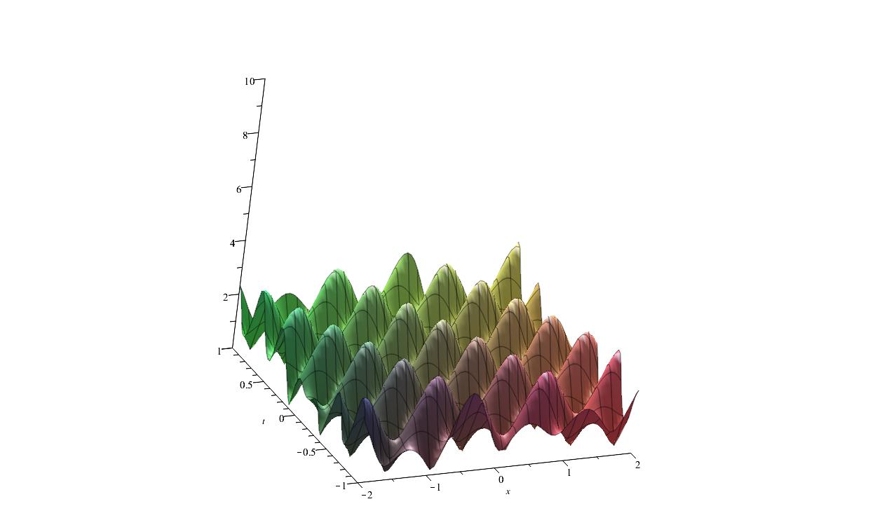
Figure 1: Modulus of a solution of the NLS equation (1) with maximum 3 and minimum 0.

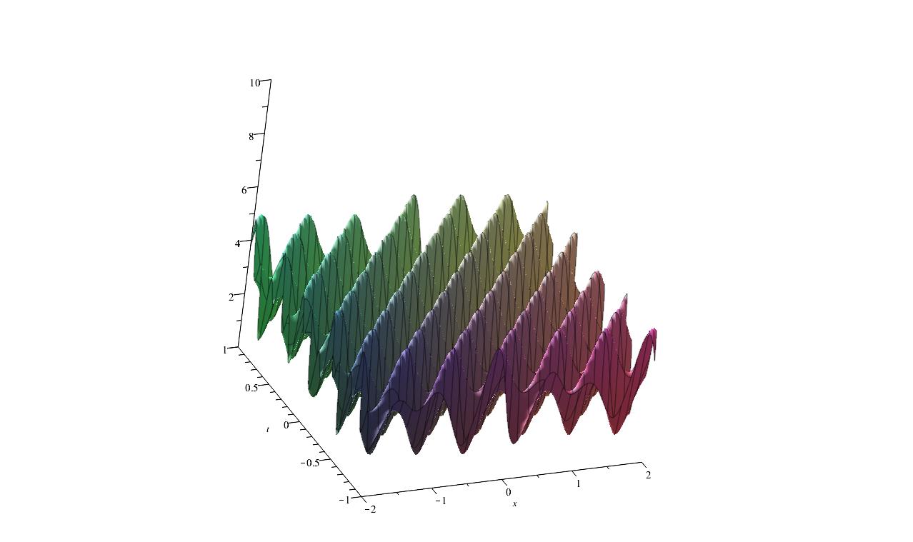
Figure 2: Modulus of a solution of the NLS equation (1) with maximum 5 and minimum 1.

10 Conclusion

An explicit parametrization of all smooth two-phase solutions of the scalar cubic NLS equation (1) is given in terms of the branch points of the invariant spectral curve and the loci of the Dirichlet eigenvalues. In particular, simple formulas are found, in terms of the imaginary parts of the branch points, for the maximum modulus and the minimum modulus of each smooth two-phase solution. Independently, a general theta function formula for the solution is given with parametrization in terms of the branch points of the genus-two Riemann surface and the values of the Dirichlet eigenvalues which satisfy the reality condtions.

The dependence of the maximum modulus of the two-phase solution on the imaginary parts of the branch points is consistent with known results for zero-phase and one-phase solutions [1] and with numerical simulations of two-phase solutions [10, 19]. For higher-phase solutions of the scalar cubic NLS equation (1), the two-real dimensional linear flow on the Jacobi variety will not span the higher-dimensional real torus of solutions, as it does in the two-dimensional case, so the sum of the imaginary parts of the branch points will be an upper bound on the modulus of the quasi-periodic solution, not necessarily the maximum value.

The parametrization obtained in this manuscript may be useful in characterizing modulations of two-phase solutions, for example, in the vicinity of a gradient catastrophe in which spikes are formed which are limits of two-phase solutions [9, 10]. More work is needed to extend the current results to the scalar defocusing cubic NLS equation and the Manakov system of coupled NLS equations [14, 15, 22, 23].

It is well-known (see [2, 6] and the references therein) how to obtain the solution of the NLS equation $p(x,t)$ in terms of theta functions defined on the Jacobi variety of the Riemann surface $\mathscr{K}_{2},$ by examining the asymptotic expansion of the Baker-Akhiezer solution of the Lax pair. In that approach, constants of integration are chosen in a manner sufficient to satisfy the reality conditions. In this paper, necessary and sufficient conditions for the existence of smooth two-phase solutions are derived for all the integration constants, using the explicit representation of the $\mu$-trajectories of the Dirichlet eigenvalues, analogous to the results for elliptic solutions obtained by Kamachatnov [1, 16]. Consequently, a theta function representation of the solution $p(x,t)$ is also constructed, using the classical integration of the Abelian integrals by the Kleinian ultra-elliptic functions, with all constants of integration expressed in terms of the branch points of the Riemann surface.

11 Appendix - The Jacobi Inversion Problem

The inversion of the Abelian integrals in equation (32) for $\mu_{1}=\mu_{1}(x,t)$ and $\mu_{2}=\mu_{2}(x,t)$ is called the Jacobi inversion problem. Classically [17] the inversion problem for the symmetric polynomials $\mu_{1}+\mu_{2}$ and $\mu_{1}\mu_{2}$ was solved in terms of the Kleinian sigma and zeta functions defined on the odd-degree genus-two curves which generalize the more familiar elliptic functions, i.e., the Weierstrass sigma and zeta functions. A more modern treatment [18] shows how the Kleinian elliptic functions can be used to solve the inversion problem for even-degree hyperelliptic curves such as $\mathscr{K}_{2}.$

11.1 Differential Identities on the Riemann Surface

In order to solve the Jacobi inversion problem (32), several definitions and fundamental identities involving differentials on the Riemann surface are needed. The goal of the present manuscript is to keep technicalities to a minimum and follow as closely as possible the classical approach of Baker [17], while using the more modern language found in [6] and [18]. First a canonical basis of homology cycles, $\{\mathfrak{a}_{1},\mathfrak{a}_{2};\mathfrak{b}_{1},\mathfrak{b}_{2}\},$ is constructed on $\mathscr{K}_{2}$ satisfying the intersection properties $\mathfrak{a}_{1}\circ\mathfrak{a}_{2}=\mathfrak{b}_{1}\circ\mathfrak{b}_{2}=0$ and $\mathfrak{a}_{1}\circ\mathfrak{b}_{1}=\mathfrak{a}_{2}\circ\mathfrak{b}_{2}=1.$ The action of the natural hyperelliptic involution $\iota$ on $\mathscr{K}_{2}$ is extended in a natural way to the homology cycles, and the cycles are chosen such that

$$\begin{array}[]{rcl}\iota(\mathfrak{a}_{1})&=&-\mathfrak{a}_{1},\\ \iota(\mathfrak{a}_{2})&=&-\mathfrak{a}_{2},\\ \iota(\mathfrak{b}_{1})&=&-\mathfrak{b}_{1},\\ \iota(\mathfrak{b}_{2})&=&-\mathfrak{b}_{2}.\end{array}$$ (A-1)

In particular, the arrangement of cycles is chosen as shown in Figure 3 for the case of three complex-conjugate pairs of branch points which satisfy the reality conditions for the NLS equation (1). Similarly, the natural action of the anti-holomorphic involution $*$ on the cycles is

$$\begin{array}[]{rcl}*(\mathfrak{a}_{1})&=&-\mathfrak{a}_{1},\\ (\mathfrak{a}_{2})&=&-\mathfrak{a}_{2},\\ (\mathfrak{b}_{1})&=&\mathfrak{b}_{1}+\mathfrak{a}_{2},\\ (\mathfrak{b}_{2})&=&\mathfrak{b}_{2}+\mathfrak{a}_{1}.\end{array}$$ (A-2)

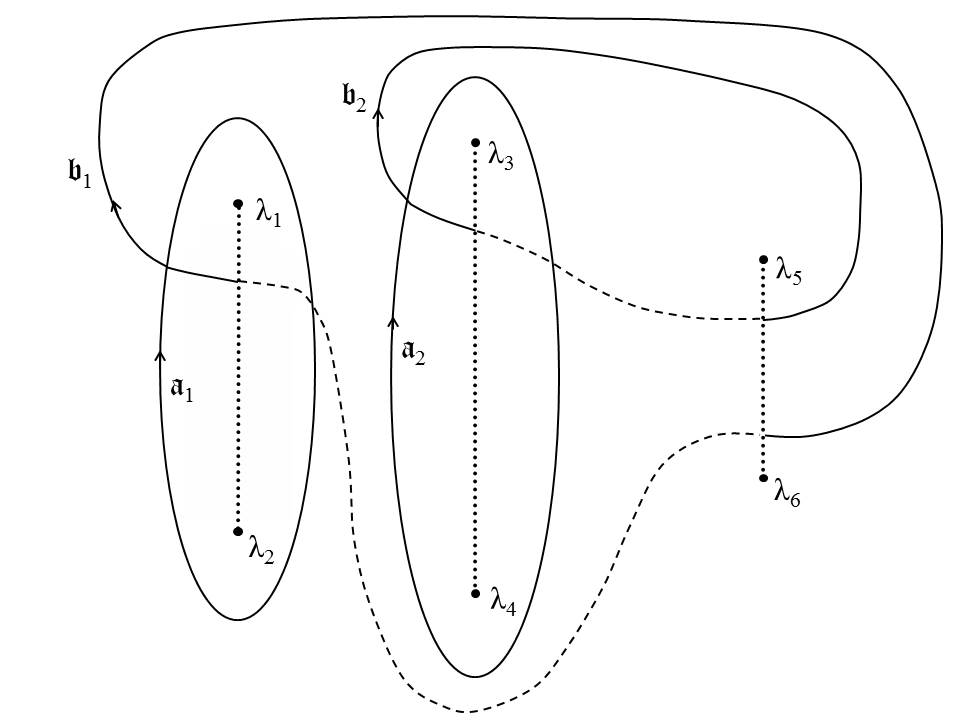
Figure 3: Basis of homology cycles, genus two, for focusing NLS equation.

Now consider the two holomorphic integrals that appear in the Jacobi inversion problem (32),

$$du_{1}=\frac{d\lambda}{w},\hskip 36.135ptdu_{2}=\frac{\lambda d\lambda}{w}.$$ (A-3)

The natural action of the anti-holomorphic involution on these two differentials is $*du_{i}=du_{i}^{*},$ for $i=1,2,$ where $du_{i}^{*}$ denotes the complex conjugate of the differential. The periods of the above differentials around the basis cycles are defined, for $i,j=1,2,$ as

$$\oint_{\mathfrak{a}_{j}}du_{i}=2\omega_{ij},\hskip 36.135pt\oint_{\mathfrak{b}_{j}}du_{i}=2\omega^{\prime}_{ij}.$$ (A-4)

Notice that for the given choice of the basis cycles,

$$\omega_{ij}^{*}=\oint_{\mathfrak{a}_{j}}du_{i}^{*}=\oint_{\mathfrak{a}_{j}}*du_{i}=\oint_{*(\mathfrak{a}_{j})}du_{i}=\oint_{-\mathfrak{a}_{j}}du_{i}=-\omega_{ij},$$ (A-5)

so that $\Re(\omega_{ij})=0.$

A normalized basis of holomorphic differentials, canonically dual to the basis of homology cycles, can now be constructed. Let, for $i=1,2,$

$$\begin{array}[]{rcl}dv_{i}&=&\sum\limits_{j=1}^{2}\frac{1}{2}(\omega^{-1})_{ij}du_{j},\end{array}$$ (A-6)

then the periods are normalized in the sense that, for $i,j=1,2,$

$$\oint_{\mathfrak{a}_{j}}dv_{i}=\delta_{ij},\hskip 36.135pt\oint_{\mathfrak{b}_{j}}dv_{i}=\tau_{ij},$$ (A-7)

where $\delta_{ij}$ is the Kronecker delta symbol. A standard result, using Riemann’s bilinear relations, is that the determinant of the matrix $\omega=(\omega_{ij})$ is nonzero, and the matrix

$$\tau=\omega^{-1}\omega^{\prime}$$ (A-8)

is symmetric with a positive definite imaginary part.

With the particular choice of the canonical cycles shown in Figure 3, the symmetry of $\mathscr{K}_{2}$ implies further information about the real part $\Re(\tau)$ of $\tau,$ viz.,

$$\begin{array}[]{rcl}\tau_{ij}^{*}&=&\oint\limits_{\mathfrak{b}_{j}}dv_{i}^{*}\\ &=&\oint\limits_{\mathfrak{b}_{j}}\sum\limits_{k=1}^{2}\frac{1}{2}(\omega^{-1})^{*}_{ik}du_{k}^{*}\\ &=&-\sum\limits_{k=1}^{2}\frac{1}{2}(\omega^{-1})_{ik}\oint\limits_{\mathfrak{b}_{j}}*du_{k}\\ &=&-\sum\limits_{k=1}^{2}\frac{1}{2}(\omega^{-1})_{ik}\oint\limits_{*(\mathfrak{b}_{j})}du_{k}\\ &=&-\sum\limits_{k=1}^{2}\frac{1}{2}(\omega^{-1})_{ik}\oint\limits_{\mathfrak{b}_{j}+\hat{\mathfrak{a}}_{j}}du_{k}\\ &=&-\sum\limits_{k=1}^{2}\frac{1}{2}(\omega^{-1})_{ik}(2\omega^{\prime}_{kj}+2\hat{\omega}_{kj})\\ &=&-\tau_{ij}-\hat{\delta}_{ij},\end{array}$$ (A-9)

where $\hat{\mathfrak{a}}_{1}=\mathfrak{a}_{2}$ and $\hat{\mathfrak{a}}_{2}=\mathfrak{a}_{1},$ so that the first and second columns of $\hat{\omega}$ are the same as the second and first columns, respectively, of $\omega,$ and

$$\hat{\delta}_{ij}=\left(\begin{array}[]{cc}0&1\\ 1&0\end{array}\right).$$ (A-10)

Therefore

$$\Re(\tau)=-\frac{1}{2}\left(\begin{array}[]{cc}0&1\\ 1&0\end{array}\right).$$ (A-11)

We now introduce two differentials of the second kind associated with $du_{1}$ and $du_{2},$ see [17], viz.,

$$dr_{1}=\frac{4\lambda^{4}-3\Lambda_{1}\lambda^{3}+2\Lambda_{2}\lambda^{2}-\Lambda_{3}\lambda}{4w}d\lambda,\hskip 28.90755ptdr_{2}=\frac{2\lambda^{3}-\Lambda_{1}\lambda^{2}}{4w}d\lambda.$$ (A-12)

These differentials are holomorphic except for poles of the second kind at the points at infinity, and they satisfy the following identity of two-differentials,

$$\frac{\partial}{\partial z}\frac{w+s}{\lambda-z}\frac{1}{2w}dz\,d\lambda+du_{1}(\lambda)dr_{1}(z)+du_{2}(\lambda)dr_{2}(z)=\frac{F(\lambda,z)+2ws}{4(\lambda-z)^{2}}\frac{d\lambda}{w}\frac{dz}{s},$$ (A-13)

where $w^{2}=\mathscr{R}(\lambda),s^{2}=\mathscr{R}(z),$ and the symmetric function $F(\lambda,z)=F(z,\lambda),$ where

$$F(\lambda,z)=2\Lambda_{6}-\Lambda_{5}(\lambda+z)+\lambda z(2\Lambda_{4}-\Lambda_{3}(\lambda+z))+\lambda^{2}z^{2}(2\Lambda_{2}-\Lambda_{1}(\lambda+z))+2\lambda^{3}z^{3}.$$ (A-14)

The periods of the differentials $dr_{1}$ and $dr_{2}$ are defined, for $i,j=1,2,$ as

$$\oint_{\mathfrak{a}_{j}}dr_{i}=-2\eta_{ij},\hskip 36.135pt\oint_{\mathfrak{b}_{j}}dr_{i}=-2\eta^{\prime}_{ij}.$$ (A-15)

The periods satisfy the following relations,

$$\begin{array}[]{ccc}\omega\omega^{\prime\,T}-\omega^{\prime}\omega^{T}&=&0,\\ \eta\eta^{\prime\,T}-\eta^{\prime}\eta^{T}&=&0,\\ \omega\eta^{\prime\,T}-\omega^{\prime}\eta^{T}&=&-\frac{\pi i}{2}\mbox{\bf I},\end{array}$$ (A-16)

where $\omega^{T}$ denotes the transpose of the matrix $\omega,$ and I is the $2\times 2$ identity matrix. Equation (A-13) shows that the symmetric two-differential on the right-hand side of the equation gives Klein’s symmetric integral of the third kind,

$$\mathscr{K}(\lambda,a;z,b)=\int\limits_{a}^{\lambda}\int\limits_{b}^{z}\frac{F(\lambda,z)+2ws}{4(\lambda-z)^{2}}\frac{d\lambda}{w}\frac{dz}{s},$$ (A-17)

with logarithmic infinities of coefficients $1$ and $-1$ respectively at $\lambda=z$ and $\lambda=b.$ Notice that the symmetry of the integrand implies that $\mathscr{K}(\lambda,a;z,b)=\mathscr{K}(z,b;\lambda,a).$

Definition 2.

The normalized differential of the third kind having a simple pole of residue $+1$ at the location $\lambda=z,$ simple pole with residue $-1$ at the location $\lambda=b,$ and zero periods around the cycles $\mathfrak{a}_{1}$ and $\mathfrak{a}_{2}$ is denoted by $d\Pi_{z,b}.$ The normalized differential of the second kind having a single pole of order two at $\lambda=z$ with coefficient $1$ and zero periods around the cycles $\mathfrak{a}_{1}$ and $\mathfrak{a}_{2}$ is denoted by $d\Gamma_{z}.$

Notice that $d\Gamma_{z}$ can be obtained from $d\Pi_{z,b}$ by differentiation of the latter with respect to the parameter $z.$ Thus an application of Riemann’s bilinear relations using $dv_{i},$ $i=1,2,$ and $d\Pi_{z,b}$ shows that

$$\oint_{\mathfrak{b}_{1}}d\Gamma_{z}=2\pi i\frac{dv_{1}}{dz}(z),\hskip 21.68121pt\oint_{\mathfrak{b}_{2}}d\Gamma_{z}=2\pi i\frac{dv_{2}}{dz}(z).$$ (A-18)

Another application of Riemann’s bilinear relations to $d\Pi_{\lambda,a}$ and $d\Pi_{z,b},$ demonstrates the following symmetry,

$$\int_{a}^{\lambda}d\Pi_{z,b}=\int_{b}^{z}d\Pi_{\lambda,a}.$$ (A-19)

Since $\mathscr{K}(\lambda,a;z,b)$ is an integral of the third kind, it can be written in terms of the normalized integral of the third kind and two linearly independent integrals of the first kind, leading to the following definition, in which the symmetry of $\mathscr{K}$ and equation (A-19) are used.

Definition 3.

Let $\alpha$ be the $2\times 2$ symmetric matrix defined by the identity

$$\mathscr{K}(\lambda,a;z,b)=\int_{a}^{\lambda}d\Pi_{z,b}-2\sum\limits_{i=1}^{2}\sum\limits_{j=1}^{2}\alpha_{ij}\int_{a}^{\lambda}du_{i}\int_{b}^{z}du_{j}.$$ (A-20)

Differentiation of the above identity with respect to local parameters $\lambda$ and $z$ gives the following identity between two-differentials,

$$\frac{F(\lambda,z)+2ws}{4(\lambda-z)^{2}}\frac{d\lambda}{w}\frac{dz}{s}=d\Gamma_{z}(\lambda)dz-2\sum\limits_{i=1}^{2}\sum\limits_{j=1}^{2}\alpha_{ij}du_{i}(\lambda)du_{j}(z).$$ (A-21)

If the roles of $\lambda$ and $z$ are interchanged in equation (A-13), using the symmetry of the two-form on the right-hand side, then equation (A-21), can be re-written as

$$du_{1}(z)dr_{1}(\lambda)+du_{2}(z)dr_{2}(\lambda)+2\sum\limits_{i=1}^{2}\sum\limits_{j=1}^{2}\alpha_{ij}du_{i}(\lambda)du_{j}(z)=d\Gamma_{z}(\lambda)dz-\frac{\partial}{\partial\lambda}\frac{s+w}{z-\lambda}\frac{d\lambda dz}{2s}.$$ (A-22)

Integration in $\lambda$ of Equation (A-22) about the basis cycles $\mathfrak{a}_{k}$ and $\mathfrak{b}_{k},$ for $k=1,2,$ gives two identities of the following differentials of $z,$

$$\begin{array}[]{rcl}-2\eta_{1k}du_{1}-2\eta_{2k}du_{2}+4\sum\limits_{i=1}^{2}\sum\limits_{j=1}^{2}\alpha_{ij}\,\omega_{ik}\,du_{j}&=&0,\\ -2\eta_{1k}^{\prime}du_{1}-2\eta_{2k}^{\prime}du_{2}+4\sum\limits_{i=1}^{2}\sum\limits_{j=1}^{2}\alpha_{ij}w_{ik}^{\prime}du_{j}&=&2\pi i\,dv_{k}\end{array}$$ (A-23)

Since $du_{1}$ and $du_{2}$ are linearly independent, the first of the identities in Equation (A-23) implies

$$\begin{array}[]{rcl}-2\eta_{1k}+4\alpha_{11}\omega_{1k}+4\alpha_{21}\omega_{2k}&=&0,\\ -2\eta_{2k}+4\alpha_{12}\omega_{1k}+4\alpha_{22}\omega_{2k}&=&0.\end{array}$$ (A-24)

Since $\alpha_{12}=\alpha_{21},$ the preceding equations imply a key relation between the period matrices of the differentials $\{du_{1},du_{2}\}$ and $\{dr_{1},dr_{2}\}$ which will be essential in defining the Kleinian sigma function, viz.,

$$\alpha=\frac{1}{2}\eta\omega^{-1}.$$ (A-25)

11.2 Riemann Theta Functions

The Kleinian sigma function will be defined using the Riemann theta function associated with the period matrix $\tau$ of the normalized differentials $dv_{1}$ and $dv_{2}.$

Definition 4.

The theta function of $v\in\mathbb{C}^{2},$ associated with the period matrix $\tau,$ is

$$\begin{array}[]{rcl}\theta(v)&=&\sum\limits_{n_{1}=-\infty}^{\infty}\sum\limits_{n_{2}=-\infty}^{\infty}e^{2\pi i(v_{1}n_{1}+v_{2}n_{2})+\pi i(\tau_{11}n_{1}^{2}+2\tau_{12}n_{1}n_{2}+\tau_{22}n_{2}^{2})}\\ &=&\sum\limits_{n=-\infty}^{\infty}e^{2\pi inv+\pi in\tau n},\end{array}$$ (A-26)

with quasiperiodicity on the period lattice $\mathbb{C}^{2}/(I\bigoplus\tau)$ given by

$$\theta(v+m+\tau m^{\prime})=e^{-2\pi im^{\prime}(v+\frac{1}{2}\tau m^{\prime})}\theta(v),$$ (A-27)

where $m,m^{\prime}\in\mathbb{Z}^{2}.$

Definition 5.

The partial derivatives of $\theta$ are denoted by

$$\begin{array}[]{rcl}\theta_{1}(v)&=&\frac{\partial\theta}{\partial v_{1}}(v),\\[7.22743pt] \theta_{2}(v)&=&\frac{\partial\theta}{\partial v_{2}}(v).\end{array}$$ (A-28)

Moreover, the logarithmic derivatives of $\theta$ possess lattice transformations of the form, for $j=1,2,$

$$\frac{\partial\ln\theta}{\partial v_{j}}(v+m+\tau m^{\prime})=-2\pi im_{j}^{\prime}+\frac{\partial\ln\theta}{\partial v_{j}}(v).$$ (A-29)

Lemma 24.

The choice of the canonical cycles obeying the conjugate relations (A-2) implies that the real part of $\tau$ satisfies equation (A-11) and, hence, it can be shown that

$$\theta(v)^{*}=\theta(v^{*}).$$ (A-30)

Similarly, for $i=1,2,$

$$\begin{array}[]{rcl}\theta_{1}(v)^{*}&=&\theta_{1}(v^{*}),\\ \theta_{2}(v)^{*}&=&\theta_{2}(v^{*}).\end{array}$$ (A-31)

Theorem 9.

The theta function is zero at odd half-integer periods, viz., if $m,m^{\prime}\in\mathbb{Z}^{2}$ and $mm^{\prime}=m_{1}m_{1}^{\prime}+m_{2}m_{2}^{\prime}$ is an odd integer, then

$$\theta(\frac{1}{2}m+\frac{1}{2}\tau m^{\prime})=0.$$

Proof.

$$\begin{array}[]{rcl}\theta(\frac{1}{2}m+\frac{1}{2}\tau m^{\prime})&=&\sum\limits_{n=-\infty}^{\infty}e^{\pi imn+\pi i(n+\frac{1}{2}m^{\prime})\tau(n+\frac{1}{2}m^{\prime})-\frac{\pi i}{4}m^{\prime}\tau m^{\prime}},\\ &=&\sum\limits_{n=-\infty}^{\infty}e^{-\pi imn+\pi i(n-\frac{1}{2}m^{\prime})\tau(n-\frac{1}{2}m^{\prime})-\frac{\pi i}{4}m^{\prime}\tau m^{\prime}},\\ &=&e^{-i\pi mm^{\prime}}\sum\limits_{n=-\infty}^{\infty}e^{-\pi im(n-m^{\prime})+\pi i(n-m^{\prime}+\frac{1}{2}m^{\prime})\tau(n-m^{\prime}+\frac{1}{2}m^{\prime})-\frac{\pi i}{4}m^{\prime}\tau m^{\prime}},\\ &=&e^{-i\pi mm^{\prime}}\sum\limits_{n=-\infty}^{\infty}e^{-\pi imn+\pi i(n+\frac{1}{2}m^{\prime})\tau(n+\frac{1}{2}m^{\prime})-\frac{\pi i}{4}m^{\prime}\tau m^{\prime}},\\ &=&e^{-i\pi mm^{\prime}}\sum\limits_{n=-\infty}^{\infty}e^{-2\pi imn+\pi imn+\pi i(n+\frac{1}{2}m^{\prime})\tau(n+\frac{1}{2}m^{\prime})-\frac{\pi i}{4}m^{\prime}\tau m^{\prime}},\\ &=&e^{-i\pi mm^{\prime}}\sum\limits_{n=-\infty}^{\infty}e^{\pi imn+\pi i(n+\frac{1}{2}m^{\prime})\tau(n+\frac{1}{2}m^{\prime})-\frac{\pi i}{4}m^{\prime}\tau m^{\prime}},\\ &=&e^{-i\pi mm^{\prime}}\theta(\frac{1}{2}m+\frac{1}{2}\tau m^{\prime}),\\ \end{array}$$ (A-32)

where the summation index is renamed, firstly, $n\rightarrow-n$ and, secondly, $n\rightarrow n-m^{\prime},$ without change to the sum, which is over all possible integer pairs $n\in\mathbb{Z}^{2}.$ ∎

Definition 6.

The half-integer periods are denoted as

$$\frac{1}{2}\left[\begin{array}[]{cc}m_{1}^{\prime}&m_{2}^{\prime}\\ m_{1}&m_{2}\end{array}\right]=\frac{1}{2}\left(\begin{array}[]{c}m_{1}+\tau_{11}m_{1}^{\prime}+\tau_{12}m_{2}^{\prime}\\ m_{2}+\tau_{21}m_{1}^{\prime}+\tau_{22}m_{2}^{\prime})\end{array}\right)=\frac{1}{2}m+\frac{1}{2}\tau m^{\prime},$$ (A-33)

where $m,m^{\prime}\in\mathbb{Z}^{2}.$

Theorem 10.

The fifteen integrals

$$v^{\lambda_{i},\lambda_{j}}=\int_{\lambda_{j}}^{\lambda_{i}}dv,$$ (A-34)

for $i,j=1,\ldots,6,$ with $i\neq j,$ of the normalized holomorphic differentials $dv=(dv_{1},dv_{2})^{t}$ on the dissected Riemann surface $\mathscr{R}$ constructed from the canonical homology cycles in Figure 3 between the fifteen pairs of distinct branch points of the Riemann surface $\mathscr{R}$ are equal to fifteen distinct non-zero half-integer periods, as follows,

$$\begin{array}[]{rclrclrcl}v^{\lambda_{1},\lambda_{2}}&=&\frac{1}{2}\left[\begin{array}[]{cc}0&0\\ 1&0\end{array}\right],&v^{\lambda_{1},\lambda_{3}}&=&\frac{1}{2}\left[\begin{array}[]{cc}-1&1\\ 0&-1\end{array}\right],&v^{\lambda_{1},\lambda_{4}}&=&\frac{1}{2}\left[\begin{array}[]{cc}-1&1\\ 0&0\end{array}\right],\\ v^{\lambda_{1},\lambda_{5}}&=&\frac{1}{2}\left[\begin{array}[]{cc}-1&0\\ 0&-1\end{array}\right],&v^{\lambda_{1},\lambda_{6}}&=&\frac{1}{2}\left[\begin{array}[]{cc}-1&0\\ 1&0\end{array}\right],&v^{\lambda_{2},\lambda_{3}}&=&\frac{1}{2}\left[\begin{array}[]{cc}-1&1\\ -1&-1\end{array}\right],\\ v^{\lambda_{2},\lambda_{4}}&=&\frac{1}{2}\left[\begin{array}[]{cc}-1&1\\ -1&0\end{array}\right],&v^{\lambda_{2},\lambda_{5}}&=&\frac{1}{2}\left[\begin{array}[]{cc}-1&0\\ -1&-1\end{array}\right],&v^{\lambda_{2},\lambda_{6}}&=&\frac{1}{2}\left[\begin{array}[]{cc}-1&0\\ 0&0\end{array}\right],\\ v^{\lambda_{3},\lambda_{4}}&=&\frac{1}{2}\left[\begin{array}[]{cc}0&0\\ 0&1\end{array}\right],&v^{\lambda_{3},\lambda_{5}}&=&\frac{1}{2}\left[\begin{array}[]{cc}0&-1\\ 0&0\end{array}\right],&v^{\lambda_{3},\lambda_{6}}&=&\frac{1}{2}\left[\begin{array}[]{cc}0&-1\\ 1&1\end{array}\right],\\ v^{\lambda_{4},\lambda_{5}}&=&\frac{1}{2}\left[\begin{array}[]{cc}0&-1\\ 0&-1\end{array}\right],&v^{\lambda_{4},\lambda_{6}}&=&\frac{1}{2}\left[\begin{array}[]{cc}0&-1\\ 1&0\end{array}\right],&v^{\lambda_{5},\lambda_{6}}&=&\frac{1}{2}\left[\begin{array}[]{cc}0&0\\ 1&1\end{array}\right].\\ \end{array}$$ (A-35)

Proof.

By examining the dissection of the Riemann surface $\mathscr{R}$ given by Figure 3, it is possible to integrate between any two branch points on the dissected Riemann surface while remaining on the lower sheet of the two-sheeted covering, without crossing any of the basis cycles. However the same integral can be performed by tracing the same path projected on the upper sheet for which the integrand is the same except for multiplication by $-1$ due to the action of the hyperelliptic involution on $dv.$ By keeping track of the crossings of the homology cycles on the upper sheet (so as to remain on the dissected Riemann surface), the equality of the two integration procedures leads to the stated results. ∎

Corollary 5.

$$\theta(v^{\lambda_{1},\lambda_{3}})=\theta(v^{\lambda_{1},\lambda_{6}})=\theta(v^{\lambda_{2},\lambda_{4}})=\theta(v^{\lambda_{2},\lambda_{5}})=\theta(v^{\lambda_{3},\lambda_{6}})=\theta(v^{\lambda_{4},\lambda_{5}})=0.$$ (A-36)

Lemma 25.

If $\theta(\int^{\lambda}_{\lambda_{6}}dv)$ is not identically zero, then it has precisely two simple zeros at $\lambda=\lambda_{1},\lambda_{3}.$

Note that $\theta(0)$ certainly does not vanish identically for all $\theta$ since $\theta(0)>0$ when $\tau=\left(\begin{array}[]{cc}i&0\\ 0&i\end{array}\right).$ In such cases $\theta(\int^{\lambda}_{\lambda_{6}}dv)$ is not identically zero, since it is not zero at $\lambda=\lambda_{6}.$

Lemma 26.

If $\theta(\int^{\lambda}_{\lambda_{6}}dv)$ is not identically zero and $z_{1}\neq z_{2},$ then $\theta(\int_{\lambda_{6}}^{\lambda}dv-\int_{\lambda_{1}}^{z_{1}}dv-\int_{\lambda_{3}}^{z_{2}}dv)$ has precisely two simple zeros at $\lambda=z_{1},z_{2}\in\mathscr{R}.$

Lemma 27.

If $\theta(\int^{\lambda}_{\lambda_{6}}dv)$ is not identically zero, then $\theta(z)=0$ if and only if $\lambda\in\mathscr{R}$ such that

$$z=\int^{\lambda}_{\lambda_{6}}dv+\int^{\lambda_{1}}_{\lambda_{3}}dv.$$

The set of $z\in\mathbb{C}^{2}/(I\bigoplus\tau)$ having this property is called the theta divisor $\Theta.$ The theta divisor is a one-complex-dimensional subvariety of the two-complex-dimensional period lattice $\mathbb{C}^{2}/(I\bigoplus\tau).$

Lemma 28.

Suppose $\theta(\int^{\lambda}_{\lambda_{6}}dv)$ is not identically zero and $e\notin\Theta,$ then $\theta(\int^{\lambda}_{\lambda_{6}}dv-e)$ is not identically zero and has precisely two zeros $\lambda=z_{1},z_{2}.$ Moreover, up to addition of integer multiples of periods,

$$e=\int_{\lambda_{1}}^{z_{1}}dv+\int_{\lambda_{3}}^{z_{2}}dv.$$ (A-37)

Thus, with the exception of the one-complex-dimensional variety $e\in\Theta,$ the points $(z_{1},s_{1}),(z_{2},s_{2})\in\mathscr{R}$ that satisfy Equation (A-37) may be viewed as well-defined functions of the independent variable $e\in\mathbb{C}^{2}/(I\bigoplus\tau).$

11.3 Kleinian elliptic functions

Definition 7.

The fundamental Kleinian sigma function $\sigma$ of $u\in\mathbb{C}^{2}$ is

$$\sigma(u)=e^{\frac{1}{2}u\eta\omega^{-1}u}\theta(\frac{1}{2}\omega^{-1}u),$$ (A-38)

with transformations on the period lattice $\mathbb{C}^{2}/(2\omega\bigoplus 2\omega^{\prime})$ given by, for $r=1,2,$

$$\begin{array}[]{ccc}\sigma(u_{1}+2\omega_{1r},u_{2}+2\omega_{2r})=e^{2\eta_{1r}(u_{1}+\omega_{1r})+2\eta_{2r}(u_{2}+\omega_{2r})}\sigma(u),\\ \sigma(u_{1}+2\omega^{\prime}_{1r},u_{2}+2\omega^{\prime}_{2r})=e^{2\eta^{\prime}_{1r}(u_{1}+\omega^{\prime}_{1r})+2\eta^{\prime}_{2r}(u_{2}+\omega^{\prime}_{2r})}\sigma(u).\end{array}$$ (A-39)

In general, if $m=(m_{1},m_{2})^{T}$ and $m^{\prime}=(m_{1}^{\prime},m_{2}^{\prime})^{T}$ are two couples of integers and

$$\Omega_{m}=2\omega m+2\omega^{\prime}m^{\prime},\hskip 14.45377ptH_{m}=2\eta m+2\eta^{\prime}m^{\prime},$$ (A-40)

then

$$\sigma(u+\Omega_{m})=e^{H_{m}(u+\frac{1}{2}\Omega_{m})-i\pi mm^{\prime}}\sigma(u).$$ (A-41)

Note that the sigma function can be multiplied by a constant factor independent of $u$ without altering any of the results of this paper. The simplest normalization sufficient to accomplish the Jacobi inversion has been chosen. The definition of the Kleinian sigma function is motivated by the following identities between integrals on the Riemann surface.

Firstly, Equation (A-20) implies

$$\begin{split}\mathscr{K}(\lambda,a;z_{1},b_{1})+\mathscr{K}(\lambda,a;z_{2},b_{2})-\int_{a}^{\lambda}d\Pi_{z_{1},b_{1}}-\int_{a}^{\lambda}d\Pi_{z_{2},b_{2}}=\\ -2\sum\limits_{i=1}^{2}\sum\limits_{j=1}^{2}\alpha_{ij}\int^{\lambda}_{a}du_{i}\left(\int_{b_{1}}^{z_{1}}du_{j}+\int_{b_{2}}^{z_{2}}du_{j}\right).\end{split}$$ (A-42)

Secondly, the identity

$$\begin{split}\int_{a}^{\lambda}d\Pi_{z_{1},b_{1}}+\int_{a}^{\lambda}d\Pi_{z_{2},b_{2}}=\\ \log\frac{\theta(\int_{\lambda_{6}}^{\lambda}dv-\int_{\lambda_{1}}^{z_{1}}dv-\int_{\lambda_{3}}^{z_{2}}dv)\theta(\int_{\lambda_{6}}^{a}dv-\int_{\lambda_{1}}^{b_{1}}dv-\int_{\lambda_{3}}^{b_{2}}dv)}{\theta(\int_{\lambda_{6}}^{\lambda}dv-\int_{\lambda_{1}}^{b_{1}}dv-\int_{\lambda_{3}}^{b_{2}}dv)\theta(\int_{\lambda_{6}}^{a}dv-\int_{\lambda_{1}}^{z_{1}}dv-\int_{\lambda_{3}}^{z_{2}}dv)},\end{split}$$ (A-43)

follows from considering the function

$$\frac{\theta(\int_{\lambda_{6}}^{\lambda}dv-\int_{\lambda_{1}}^{z_{1}}dv-\int_{\lambda_{3}}^{z_{2}}dv)}{\theta(\int_{\lambda_{6}}^{\lambda}dv-\int_{\lambda_{1}}^{b_{1}}dv-\int_{\lambda_{3}}^{b_{2}}dv)}\exp\left(-\int_{a}^{\lambda}d\Pi_{z_{1},b_{1}}-\int_{a}^{\lambda}d\Pi_{z_{2},b_{2}}\right),$$

which must be constant because it has no zeros and no poles and zero periods around all homology basis cycles. Therefore it is equal to its value when $\lambda=a.$ A similar conclusion follows even if only the periods around $\mathfrak{a}_{1}$ and $\mathfrak{a}_{2}$ are zero and the periods around $\mathfrak{b}_{1}$ and $\mathfrak{b}_{2}$ are constant (but not necessarily zero).

The two identities in Equations (A-42) and (A-43) can be written in terms of the Kleinian sigma function (A-38), using the fact that $\alpha=\frac{1}{2}\eta\omega^{-1},$ as

$$\begin{split}\mathscr{K}(\lambda,a;z_{1},b_{1})+\mathscr{K}(\lambda,a;z_{2},b_{2})=\\ \log\frac{\sigma(\int_{\lambda_{6}}^{\lambda}du-\int_{\lambda_{1}}^{z_{1}}du-\int_{\lambda_{3}}^{z_{2}}du)\sigma(\int_{\lambda_{6}}^{a}du-\int_{\lambda_{1}}^{b_{1}}du-\int_{\lambda_{3}}^{b_{2}}du)}{\sigma(\int_{\lambda_{6}}^{\lambda}du-\int_{\lambda_{1}}^{b_{1}}du-\int_{\lambda_{3}}^{b_{2}}du)\sigma(\int_{\lambda_{6}}^{a}du-\int_{\lambda_{1}}^{z_{1}}du-\int_{\lambda_{3}}^{z_{2}}du)},\end{split}$$ (A-44)

where $du=(du_{1},du_{2})^{T}$ and $dv=(dv_{1},dv_{2})^{T}.$

Now Equation (A-13), in which we interchange $(\lambda,a)$ and $(z,b)$ using the symmetry of the expression, and Equation (A-17) imply

$$\begin{split}\mathscr{K}(\lambda,a;z_{1},b_{1})+\mathscr{K}(\lambda,a;z_{2},b_{2})=\int_{b_{1}}^{z_{1}}\int_{a}^{\lambda}\frac{\partial}{\partial\lambda}\frac{s+w}{z-\lambda}\frac{d\lambda}{2s}dz+\\ \int_{b_{2}}^{z_{2}}\int_{a}^{\lambda}\frac{\partial}{\partial\lambda}\frac{s+w}{z-\lambda}\frac{d\lambda}{2s}dz+\left(\int_{b_{1}}^{z_{1}}du_{1}+\int_{b_{2}}^{z_{2}}du_{1}\right)\int_{a}^{\lambda}dr_{1}+\\ \left(\int_{b_{1}}^{z_{1}}du_{2}+\int_{b_{2}}^{z_{2}}du_{2}\right)\int_{a}^{\lambda}dr_{2}.\end{split}$$ (A-45)

The identities in Equations (A-44) and (A-45) combine to give

$$\begin{split}\log\frac{\sigma(\int_{\lambda_{6}}^{\lambda}du-\int_{\lambda_{1}}^{z_{1}}du-\int_{\lambda_{3}}^{z_{2}}du)\sigma(\int_{\lambda_{6}}^{a}du-\int_{\lambda_{1}}^{b_{1}}du-\int_{\lambda_{3}}^{b_{2}}du)}{\sigma(\int_{\lambda_{6}}^{\lambda}du-\int_{\lambda_{1}}^{b_{1}}du-\int_{\lambda_{3}}^{b_{2}}du)\sigma(\int_{\lambda_{6}}^{a}du-\int_{\lambda_{1}}^{z_{1}}du-\int_{\lambda_{3}}^{z_{2}}du)}=\\ \int_{b_{1}}^{z_{1}}\int_{a}^{\lambda}\frac{\partial}{\partial\lambda}\frac{s+w}{z-\lambda}\frac{d\lambda}{2s}dz+\int_{b_{2}}^{z_{2}}\int_{a}^{\lambda}\frac{\partial}{\partial\lambda}\frac{s+w}{z-\lambda}\frac{d\lambda}{2s}dz+\\ \left(\int_{b_{1}}^{z_{1}}du_{1}+\int_{b_{2}}^{z_{2}}du_{1}\right)\int_{a}^{\lambda}dr_{1}+\left(\int_{b_{1}}^{z_{1}}du_{2}+\int_{b_{2}}^{z_{2}}du_{2}\right)\int_{a}^{\lambda}dr_{2}.\end{split}$$ (A-46)

Lemma A-37 and the discussion following Equation (A-43) shows that in Equation (A-46), for $u^{\prime},u^{\prime\prime}\notin\Theta,$ we can write

$$u^{\prime}=\int_{\lambda_{1}}^{z_{1}}du+\int_{\lambda_{3}}^{z_{2}}du,\hskip 14.45377ptu^{\prime\prime}=\int_{\lambda_{1}}^{b_{1}}du+\int_{\lambda_{3}}^{b_{2}}du,$$

consider $z_{1}$ and $z_{2}$ as functions of $u^{\prime}$ and $b_{1}$ and $b_{2}$ as functions of $u^{\prime\prime}.$ Thus Equation (A-46) becomes,

$$\begin{split}\log\frac{\sigma(\int_{\lambda_{6}}^{\lambda}du-u^{\prime})\sigma(\int_{\lambda_{6}}^{a}du-u^{\prime\prime})}{\sigma(\int_{\lambda_{6}}^{\lambda}du-u^{\prime\prime})\sigma(\int_{\lambda_{6}}^{a}du-u^{\prime})}=\int_{b_{1}}^{z_{1}}\int_{a}^{\lambda}\frac{\partial}{\partial\lambda}\frac{s+w}{z-\lambda}\frac{d\lambda}{2s}dz+\\ \int_{b_{2}}^{z_{2}}\int_{a}^{\lambda}\frac{\partial}{\partial\lambda}\frac{s+w}{z-\lambda}\frac{d\lambda}{2s}dz+\left(u^{\prime}_{1}-u^{\prime\prime}_{1}\right)\int_{a}^{\lambda}dr_{1}+\left(u^{\prime}_{2}-u^{\prime\prime}_{2}\right)\int_{a}^{\lambda}dr_{2}.\end{split}$$ (A-47)

Differentiation of Equation (A-47) with respect to $u_{i}^{\prime}$ for $i=1,2,$ produces

$$\begin{split}-\zeta_{i}\left(\int^{\lambda}_{\lambda_{6}}du-u^{\prime}\right)+\zeta_{i}\left(\int^{a}_{\lambda_{6}}du-u^{\prime}\right)=\frac{\partial z_{1}}{\partial u_{i}^{\prime}}\int_{a}^{\lambda}\frac{\partial}{\partial\lambda}\frac{s_{1}+w}{z_{1}-\lambda}\frac{d\lambda}{2s_{1}}+\\ \frac{\partial z_{2}}{\partial u_{i}^{\prime}}\int^{\lambda}_{a}\frac{\partial}{\partial\lambda}\frac{s_{2}+w}{z_{2}-\lambda}\frac{d\lambda}{2s_{2}}+\int^{\lambda}_{a}dr_{i},\end{split}$$ (A-48)

where the zeta functions $\zeta_{i}$ and $\wp_{ij}$ functions for $i,j=1,2,$ are defined by

$$\zeta_{i}(u)=\frac{\partial}{\partial u_{i}}\log\sigma(u),\hskip 14.45377pt\wp_{ij}=-\frac{\partial^{2}}{\partial u_{i}\partial u_{j}}\log\sigma(u).$$ (A-49)

Equation (A-41) shows that, for $i,j=1,2,$ and $\Omega_{m}$ an integer translation across the period lattice of the Jacobi variety of $\mathscr{K}_{2},$

$$\zeta_{i}(u+\Omega_{m})-\zeta_{i}(u)=(H_{m})_{i}=2\eta_{i1}m_{1}+2\eta_{i2}m_{2}+2\eta^{\prime}_{i1}m_{1}^{\prime}+2\eta_{i2}^{\prime}m_{2}^{\prime}$$ (A-50)

and

$$\wp_{ij}(u+\Omega_{m})=\wp_{ij}(u).$$ (A-51)

Using

$$\begin{array}[]{rcl}u_{1}&=&\int^{z_{1}}_{\lambda_{1}}\frac{dz}{s}+\int^{z_{2}}_{\lambda_{3}}\frac{dz}{s},\\ u_{2}&=&\int^{z_{1}}_{\lambda_{1}}\frac{zdz}{s}+\int^{z_{2}}_{\lambda_{3}}\frac{zdz}{s},\end{array}$$ (A-52)

we find that

$$\begin{array}[]{rclrcl}\frac{\partial z_{1}}{\partial u_{1}}&=&\frac{s_{1}z_{2}}{z_{2}-z_{1}},&\hskip 14.45377pt\frac{\partial z_{2}}{\partial u_{1}}&=&\frac{s_{2}z_{1}}{z_{1}-z_{2}},\\ \frac{\partial z_{1}}{\partial u_{2}}&=&\frac{s_{1}}{z_{1}-z_{2}},&\hskip 14.45377pt\frac{\partial z_{2}}{\partial u_{2}}&=&\frac{s_{2}}{z_{2}-z_{1}}.\end{array}$$ (A-53)

In Equation (A-48) we now make the change of replacing the points $(z_{1},s_{1}),(z_{2},s_{2})\in\mathscr{K}_{2}$ with their corresponding points under the hyperelliptic involution, viz., $(z_{1},-s_{1})$ and $(z_{2},-s_{2}).$ Notice that $u_{r}^{\prime}$ is changed by this transformation to

$$-u_{r}^{\prime}+2\omega_{i1}m_{1}+2\omega_{i2}m_{2}+2\omega^{\prime}_{i1}m_{1}^{\prime}+2\omega_{i2}^{\prime}m_{2}^{\prime}$$ (A-54)

for some integers $m_{1},m_{2},m_{1}^{\prime},m_{2}^{\prime}.$ Making the corresponding change in the right-hand side of Equation (A-48) and using Equation (A-53), we obtain, for $i=1,2,$

$$\int^{\lambda}_{a}dr_{i}+\zeta_{i}\left(\int^{\lambda}_{\lambda_{6}}du+u^{\prime}\right)-\frac{1}{2}f_{i}(\lambda,z_{1},z_{2})=\zeta_{i}\left(\int^{a}_{\lambda_{6}}du+u^{\prime}\right)-\frac{1}{2}f_{i}(a,z_{1},z_{2}),$$ (A-55)

where

$$\begin{array}[]{rcl}f_{1}(\lambda,z_{1},z_{2})&=&\frac{w(\lambda-z_{1}-z_{2})}{(z_{1}-\lambda)(z_{2}-\lambda)}+\frac{s_{1}(z_{1}-\lambda-z_{2})}{(z_{1}-\lambda)(z_{1}-z_{2})}+\frac{s_{2}(z_{2}-\lambda-z_{1})}{(z_{2}-\lambda)(z_{2}-z_{1})},\\ f_{2}(\lambda,z_{1},z_{2})&=&\frac{w}{(z_{1}-\lambda)(z_{2}-\lambda)}+\frac{s_{1}}{(z_{1}-\lambda)(z_{1}-z_{2})}+\frac{s_{2}}{(z_{2}-\lambda)(z_{2}-z_{1})}.\end{array}$$ (A-56)

By adding $\int^{z_{1}}_{\lambda_{1}}dr_{i}+\int^{z_{2}}_{\lambda_{3}}dr_{i}$ to both sides of Equation (A-55), we obtain

$$\begin{split}\int^{\lambda}_{a}dr_{i}+\int^{z_{1}}_{\lambda_{1}}dr_{i}+\int^{z_{2}}_{\lambda_{3}}dr_{i}+\zeta_{i}\left(\int^{\lambda}_{\lambda_{6}}du+u^{\prime}\right)-\frac{1}{2}f_{i}(\lambda,z_{1},z_{2})\\ =\int^{z_{1}}_{\lambda_{1}}dr_{i}+\int^{z_{2}}_{\lambda_{3}}dr_{i}+\zeta_{i}\left(\int^{a}_{\lambda_{6}}du+u^{\prime}\right)-\frac{1}{2}f_{i}(a,z_{1},z_{2}),\end{split}$$ (A-57)

in which the left-hand side is symmetric with respect to $\lambda,z_{1},z_{2},$ and the right-hand side is the value of the left-hand side when $\lambda=a.$ Consequently the left-hand side of Equation (A-57) is independent of $\lambda,z_{1},$ and $z_{2}.$ Therefore, for $i=1,2,$

$$\zeta_{i}\left(\int^{\lambda}_{\lambda_{6}}du+u^{\prime}\right)=C_{i}+\frac{1}{2}f_{i}(\lambda,z_{1},z_{2})-\int^{\lambda}_{a}dr_{i}-\int^{z_{1}}_{\lambda_{1}}dr_{i}-\int^{z_{2}}_{\lambda_{3}}dr_{i},$$ (A-58)

where $C_{i}$ is independent of $\lambda,z_{1},z_{2}.$ Since $a$ is an arbitrary point on $\mathcal{K}_{2},$ it can be set equal to the branch point at $a=\lambda_{6},$ giving

$$\zeta_{i}\left(\int^{\lambda}_{\lambda_{6}}du+u^{\prime}\right)=C_{i}+\frac{1}{2}f_{i}(\lambda,z_{1},z_{2})-\int^{\lambda}_{\lambda_{6}}dr_{i}-\int^{z_{1}}_{\lambda_{1}}dr_{i}-\int^{z_{2}}_{\lambda_{3}}dr_{i},$$ (A-59)

Now $\zeta_{i}(0)=0,$ being an odd function, so setting $\lambda=\lambda_{6},z_{1}=\lambda_{1},$ and $z_{2}=\lambda_{3},$ shows that $C_{i}=0,$ for $i=1,2.$

Direct calculation shows that, as $\lambda\rightarrow\infty^{\pm},$ the singularities in the terms on the right-hand side of equation (A-59) cancel out, so that

$$\lim_{\lambda\rightarrow\infty^{\pm}}\frac{1}{2}f_{i}(\lambda,z_{1},z_{2})-\int^{\lambda}_{\lambda_{6}}dr_{i}=\gamma_{i}^{\pm},$$ (A-60)

where

$$\begin{array}[]{rcl}\gamma_{1}^{\pm}&=&\pm\frac{1}{2}(-z_{1}z_{2}-\frac{1}{8}\Lambda_{1}^{2}+\frac{1}{2}\Lambda_{2})+\frac{1}{2}\frac{s_{1}-s_{2}}{z_{1}-z_{2}}+\delta_{1}^{\pm},\\[7.22743pt] \gamma_{2}^{\pm}&=&\pm\frac{1}{2}(z_{1}+z_{2}-\frac{1}{2}\Lambda_{1})+\delta_{2}^{\pm},\end{array}$$ (A-61)

and $\delta_{1}^{\pm}$ and $\delta_{2}^{\pm}$ are constants independent of $z_{1}$ and $z_{2}.$ Thus equation (A-59) becomes

$$\zeta_{i}\left(\int^{\infty^{\pm}}_{\lambda_{6}}du+u^{\prime}\right)=\gamma_{i}^{\pm}-\int^{z_{1}}_{\lambda_{1}}dr_{i}-\int^{z_{2}}_{\lambda_{3}}dr_{i}.$$ (A-62)

Equation (A-62), implies, for $i=1,2,$

$$\begin{split}\zeta_{i}\left(u^{\prime}+\int^{\infty^{+}}_{\lambda_{6}}du\right)-\zeta_{i}\left(u^{\prime}+\int^{\infty^{-}}_{\lambda_{6}}du\right)=\gamma_{i}^{+}-\gamma_{i}^{-}\end{split}$$ (A-63)

Substituting the explicit expressions for $\gamma^{\pm}_{i},$ we obtain the solution to the Jacobi inversion problem,

$$\begin{array}[]{rcl}\zeta_{1}\left(u^{\prime}+\int^{\infty^{+}}_{\lambda_{6}}du\right)-\zeta_{1}\left(u^{\prime}+\int^{\infty^{-}}_{\lambda_{6}}du\right)&=&-z_{1}z_{2}-\frac{1}{8}\Lambda_{1}^{2}+\frac{1}{2}\Lambda_{2}+\delta_{1},\\[14.45377pt] \zeta_{2}\left(u^{\prime}+\int^{\infty^{+}}_{\lambda_{6}}du\right)-\zeta_{2}\left(u^{\prime}+\int^{\infty^{-}}_{\lambda_{6}}du\right)&=&z_{1}+z_{2}-\frac{1}{2}\Lambda_{1}+\delta_{2},\end{array}$$ (A-64)

where the constants $\delta_{1}$ and $\delta_{2}$ are independent of $z_{1}$ and $z_{2},$ and so can be obtained from equation (A-64) by setting $z_{1}=(\lambda_{1},0)$ and $z_{2}=(\lambda_{2},0)=(\lambda_{1}^{*},0).$ Recall $\alpha_{ij}$ for $i,j=1,2,$ is given by

$$\alpha=\frac{1}{2}\eta\omega^{-1}=\left(\begin{array}[]{cc}\alpha_{11}&\alpha_{12}\\[7.22743pt] \alpha_{21}&\alpha_{22}\end{array}\right).$$ (A-65)

Hence

$$\begin{array}[]{rcl}\delta_{1}=\delta_{1}^{+}-\delta_{1}^{-}&=&-(-|\lambda_{1}|^{2}-\frac{1}{8}\Lambda_{1}^{2}+\frac{1}{2}\Lambda_{2})\\ &&+\zeta_{1}\left(\int^{\infty^{+}}_{\lambda_{6}}du+\int^{\lambda_{2}}_{\lambda_{3}}du\right)-\zeta_{1}\left(\int^{\infty^{-}}_{\lambda_{6}}du+\int^{\lambda_{2}}_{\lambda_{3}}du\right)\\[7.22743pt] &=&-(-|\lambda_{1}|^{2}-\frac{1}{8}\Lambda_{1}^{2}+\frac{1}{2}\Lambda_{2})+2\alpha_{11}\int^{\infty^{+}}_{\infty^{-}}du_{1}+(\alpha_{12}+\alpha_{21})\int^{\infty^{+}}_{\infty^{-}}du_{2}\\ &&+\frac{1}{2}(\omega^{-1})_{11}(\frac{\theta_{1}^{+}}{\theta^{+}}-\frac{\theta_{1}^{-}}{\theta^{-}})+\frac{1}{2}(\omega^{-1})_{21}(\frac{\theta_{2}^{+}}{\theta^{+}}-\frac{\theta_{2}^{-}}{\theta^{-}}),\\[7.22743pt] \delta_{2}=\delta_{2}^{+}-\delta_{2}^{-}&=&-(\lambda_{1}+\lambda_{1}^{*}-\frac{1}{2}\Lambda_{1})\\ &&+\zeta_{2}\left(\int^{\infty^{+}}_{\lambda_{6}}du+\int^{\lambda_{2}}_{\lambda_{3}}\right)-\zeta_{2}\left(\int^{\infty^{-}}_{\lambda_{6}}du+\int^{\lambda_{2}}_{\lambda_{3}}du\right)\\ &=&-(\lambda_{1}+\lambda_{1}^{*}-\frac{1}{2}\Lambda_{1})+(\alpha_{12}+\alpha_{21})\int^{\infty^{+}}_{\infty^{-}}du_{1}+2\alpha_{22}\int^{\infty^{+}}_{\infty^{-}}du_{2}\\ &&+\frac{1}{2}(\omega^{-1})_{12}(\frac{\theta_{1}^{+}}{\theta^{+}}-\frac{\theta_{1}^{-}}{\theta^{-}})+\frac{1}{2}(\omega^{-1})_{22}(\frac{\theta_{2}^{+}}{\theta^{+}}-\frac{\theta_{2}^{-}}{\theta^{-}}),\end{array}$$ (A-66)

where

$$\begin{array}[]{rcl}\theta^{+}&=&\theta\left(\frac{1}{2}\omega^{-1}(\int^{\infty^{+}}_{\lambda_{6}}du+\int^{\lambda_{2}}_{\lambda_{3}}du)\right),\\[7.22743pt] \theta^{-}&=&\theta\left(\frac{1}{2}\omega^{-1}(\int^{\infty^{-}}_{\lambda_{6}}du+\int^{\lambda_{2}}_{\lambda_{3}}du)\right),\\[7.22743pt] \theta_{1}^{+}&=&\theta_{1}\left(\frac{1}{2}\omega^{-1}(\int^{\infty^{+}}_{\lambda_{6}}du+\int^{\lambda_{2}}_{\lambda_{3}}du)\right),\\[7.22743pt] \theta_{1}^{-}&=&\theta_{1}\left(\frac{1}{2}\omega^{-1}(\int^{\infty^{-}}_{\lambda_{6}}du+\int^{\lambda_{2}}_{\lambda_{3}}du)\right),\\[7.22743pt] \theta_{2}^{+}&=&\theta_{2}\left(\frac{1}{2}\omega^{-1}(\int^{\infty^{+}}_{\lambda_{6}}du+\int^{\lambda_{2}}_{\lambda_{3}}du)\right),\\[7.22743pt] \theta_{2}^{-}&=&\theta_{2}\left(\frac{1}{2}\omega^{-1}(\int^{\infty^{-}}_{\lambda_{6}}du+\int^{\lambda_{2}}_{\lambda_{3}}du)\right).\\[7.22743pt] \end{array}$$ (A-67)

Explicit expressions for $z_{1}$ and $z_{2}$ can then be found from the quadratic formula for the roots of the quadratic equation

$$z^{2}-(z_{1}+z_{2})z+z_{1}z_{2}=0.$$ (A-68)

The corresponding values of $s_{1}$ and $s_{2}$ for $(z_{1},s_{1}),(z_{2},s_{2})\in\mathscr{K}_{2}$ are, for $k=1,2,$

$$\begin{split}s_{k}=\left(\wp_{22}\left(u^{\prime}+\int^{\infty^{-}}_{\lambda_{6}}du\right)-\wp_{22}\left(u^{\prime}+\int^{\infty^{+}}_{\lambda_{6}}du\right)\right)z_{k}\\ +\wp_{12}\left(u^{\prime}+\int^{\infty^{-}}_{\lambda_{6}}du\right)-\wp_{12}\left(u^{\prime}+\int^{\infty^{+}}_{\lambda_{6}}du\right).\end{split}$$ (A-69)

References

• [1] A. M. Kamchatnov, Nonlinear Periodic Waves and Their Modulations: An Introductory Course, World Scientific, Singapore, 2000.
• [2] B. A. Dubrovin, Theta functions and non-linear equations, Russian Math. Surveys 36:2 (1981) 11-92.
• [3] E. R. Tracy, H. H. Chen, Y. C. Lee, Study of Quasiperiodic Solutions of the Nonlinear Schrödinger equation and the Nonlinear Modulational Instability, Phys. Rev. Lett. 53 (1984) 218-221.
• [4] E. Previato, Hyperelliptic Quasi-Periodic and Soliton-Solutions of the Nonlinear Schrödinger Equation, Duke Math. Journal 52 (1985) 329-377.
• [5] E. R. Tracy, H. H. Chen, Nonlinear self-modulation: An exactly solvable model, Phys. Rev. A 37 (1988) 815-839.
• [6] E. D. Belokolos, A. I. Bobenko, V. Z. Enol’skii, A. R. Its, V. B. Matveev, Algebro-Geometric Approach to Nonlinear Integrable Equations, Springer-Verlag, Berlin, 1994.
• [7] M. G. Forest, D. W. McLaughlin, Spectral theory for the periodic sineGordon equation: A concrete viewpoint , J. Math. Phys. 23 (1982) 1248-1277.
• [8] N. Ercolani, M. G. Forest, The Geometry of Real Sine-Gordon Wavetrains, Comm. Math. Phys. 99 (1985) 1-49.
• [9] M. Bertola, A. Tovbis, Universality for the Focusing Nonlinear Schrödinger Equation at the Gradient Catastrophe Point: Rational Breathers and Poles of the Tritronquee Solution to Painleve I, Comm. on Pure and Applied Math. 66 (2013) 678-752.
• [10] G. A. El, E. G. Khamis, A. Tovbis, Dam break problem for the focusing nonlinear Schrödinger equation and the generation of rogue waves, arXiv:1505.01785v1 [nlin.PS]
• [11] A. V. Porubov, D. F. Parker, Some general periodic solutions to coupled nonlinear Schrödinger equations, Wave Motion 29 (1999) 97-109.
• [12] P. L. Christiansen, J. C. Eilbeck, V. Z. Enolskii, N. A. Kostov, Quasi-periodic and periodic solutions for coupled nonlinear Schrödinger equations of the Manakov type, Proc. R. Soc. Lon. A 456 (2000) 2263-2281.
• [13] J. C. Eilbeck, V. Z. Enolskii, N. A. Kostov, Quasi-periodic and periodic solutions for vector nonlinear Schrödinger equations, J. Math. Phys. 41 (2000) 8236-8248.
• [14] T. Woodcock, O. H. Warren, J. N. Elgin, Genus two finite gap solutions of the vector nonlinear Schrödinger equation, J. Phys. A: Math. Theor. 40 (2007) F355-F361.
• [15] A. Kamchatnov, On periodic solutions and their modulations of the Manakov system, J. Phys. A 47 (2014) 145203.
• [16] A. M. Kamchatnov, On improving the effectiveness of periodic solutions of the NLS and DNLS equations, J. Phys. A: Math. Gen. 23 (1990) 2945-2960.
• [17] H. F. Baker, Multiply Periodic Functions, Cambridge University Press, Cambridge, 1907.
• [18] J. C. Eilbeck, V. Z. Enolskii, H. Holden, The Hyperelliptic $\zeta$-Function and the Integrable Massive Thirring Model, Proc. R. Soc. A, 459 (2035) (2003) 1581-1610.
• [19] A. R. Osborne, Nonlinear ocean waves and the inverse scattering transform, Elsevier, Amsterdam, 2010.
• [20] H. Flaschka, A. C. Newell, T. Ratiu, Kac-Moody Lie Algebras and Soliton Equations. 2. Lax Equations associated with A1, Physica D 9 (3) (1983) 300-323, DOI: 10.1016/0167-2789(83)90274-9.
• [21] T. Piezas, Solving Solvable Sextics using Polynomial Decomposition, 2004. http://www.oocities/titus_piezas/Sextic.pdf, downloaded October 4, 2012.
• [22] J. N. Elgin, V. Z. Enolski, A. R. Its, Effective integration of the nonlinear vector Schrödinger equation, Physica D 225 (2007) 127-152.
• [23] O. C. Wright III, On elliptic solutions of a coupled nonlinear Schrödinger equation, Physica D 264 (2013) 1-16.
• [24] B. Deconinck, M. S. Patterson, Computing with Plane Algebraic Curves and Riemann Surfaces: The Algorithms of the Maple Package “Algcurves,” pp. 67-123, in A.I. Bobenko, C. Klein (eds.), Computational Approach to Riemann Surfaces, Lecture Notes in Mathematics 2013, Springer-Verlag, Berlin, 2011.