Curvature generation in nematic surfaces

Abstract

In recent years there has been a growing interest in the study of shape formation using modern responsive materials that can be preprogrammed to undergo spatially inhomogeneous local deformations. In particular, nematic liquid crystalline solids offer exciting possibilities in this context. Considerable recent progress has been made in achieving a variety of shape transitions in thin sheets of nematic solids by engineering isolated points of concentrated Gaussian curvature using topological defects in the nematic director field across textured surfaces. In this paper, we consider ways of achieving shape transitions in thin sheets of nematic glass by generation of non-localised Gaussian curvature in the absence of topological defects in the director field. We show how one can blueprint any desired Gaussian curvature in a thin nematic sheet by controlling the nematic alignment angle across the surface and highlight specific patterns which present feasible initial targets for experimental verification of the theory.

I Introduction

Complex shape transitions driven by inhomogeneous local deformation patterns are ubiquitous in nature and are observed at a variety of length scales, ranging from the cell walls of plants and bacteria to macrostructures such as plant leaves Dervaux and Ben Amar (2008). Examples of such local deformations include differential growth in biological structures and nonuniform mechanical responses of biological tissues to external stimuli such as humidity Goriely and Moulton (2011). Modern responsive materials can be preprogrammed to undergo spatially inhomogeneous expansions and contractions in response to external stimuli such as heat and light. Examples include thermoresponsive hydrogels Klein et al. (2007) and nematic liquid crystalline solids Modes et al. (2011). There has been considerable interest in recent years in the prospect of preprogramming desired shape transformations that can be remotely activated in such materials Efrati et al. (2009); Modes and Warner (2011); Kim et al. (2012).

Liquid crystalline solids consist of long, flexible molecular chains that are sufficiently cross-linked to form a solid. At sufficiently high temperatures, the molecular directions are randomly distributed and the material is in the isotropic phase. When the temperature is below some critical value, the rod-like molecular elements become locally aligned about the director $\bm{n}$ and the material is said to be in the nematic phase. Liquid crystalline solids experience elongations and contractions in response to light, heat, pH, and other stimuli that change the molecular order. Of particular significance are nematic glasses Van Oosten et al. (2007) and elastomers Warner and Terentjev (2003). Both have spontaneous deformation tensors of the form

$$F=(\lambda-\lambda^{-\nu})\bm{n}\otimes\bm{n}+\lambda^{-\nu}\,\mathrm{Id}_{3},$$ (1)

where $\mathrm{Id}_{3}$ denotes the identity operator on $\mathbb{R}^{3}$. That is, a local scaling by $\lambda$ along the director $\bm{n}$ and a scaling by $\lambda^{-\nu}$ perpendicular to $\bm{n}$ is observed upon exposure to stimulus. The parameter $\nu$ is known as the opto-thermal Poisson ratio and relates the perpendicular and parallel responses Modes and Warner (2011).

In nematic glasses, molecular chain motion is highly limited by the cross-links and the director is not independently mobile from the elastic matrix as it is in elastomers. For nematic glasses, we typically have $\lambda\in(0.96,1.04)$ and $\nu\in(\frac{1}{2},2)$, while for elastomers $\lambda\in(\frac{1}{2},4)$ and $\nu=\frac{1}{2}$. In nematic glasses, the director field changes only through convection by mechanical deformations, which allows for a feasible patterning of the director field at the initial time of cross-linking and the subsequent guarantee that the pattern will not be modified by “soft elasticity” mediated by director rotation Warner and Terentjev (2003). Considerable control of director fields is achievable through a variety of techniques including the use of electric and magnetic fields, surface anchoring, and holography. Thus, the matrial response in nematic glasses can be preprogrammed by precisely setting up a desired director field pattern immediately before the glass is formed via cross-linking Modes and Warner (2011); Van Oosten et al. (2007).

It has come to our attention that a recent ambitious paper by Aharoni et al. Aharoni et al. (2014) addresses the question of shape transformations that are achievable through the patterning of general smooth director fields on flat sheets, as was the original motivation for much of this work. Nonetheless, we hope that this paper will add to their contribution by highlighting specific patterns which present feasible initial targets for experimental confirmations of the theory. We also introduce the notion of orthogonal duality of director fields and consider its implication for Gaussian curvature distributions. Nematic patterns on initially curved surfaces are considered towards the end of the paper.

The value of $\lambda$ and $\nu$ are typically dependent on the strength of the stimulus. In the following analysis, we assume that the shape transformation is achieved by a sudden exposure to stimulus of fixed strength, so that there is a sudden activation of the prescribed local deformations for fixed values $\lambda$ and $\nu$. For definiteness, we assume that $\lambda<1$, so that the local deformations consist of a contraction along the director and an elongation in the perpendicular directions. We use the convention that Latin indices run over 1, 2, 3, whereas Greek indices take values 1 and 2.

II Non-Euclidean local deformations and nematic surfaces

A configuration of a body in $\mathbb{R}^{3}$ can be specified by a smooth injective immersion $\bm{\Phi}:\Omega\rightarrow\mathbb{R}^{3}$, where $\Omega\subset\mathbb{R}^{3}$ is a domain. The configuration defines curvilinear coordinates $x=(x^{i})=(x^{1},x^{2},x^{3})\in\Omega$ for material points throughout the body. The map $\bm{\Phi}:\Omega\rightarrow\mathbb{R}^{3}$ induces a Riemannian metric $g$ on $\Omega$ with covariant components

$$g_{ij}(x)=\partial_{i}\bm{\Phi}\cdot\partial_{j}\bm{\Phi}.$$ (2)

The Christoffel symbols are defined in terms of the components of the metric tensor by

$$\Gamma_{ijl}=\frac{1}{2}(\partial_{j}g_{il}+\partial_{i}g_{jl}-\partial_{l}g_{ij})$$ (3)

and $\Gamma^{k}_{ij}=g^{kl}\Gamma_{ijl}$, where $(g^{ij})=(g_{ij})^{-1}$. It is well-known that the components

$$R_{lijk}=\partial_{j}\Gamma_{ikl}-\partial_{k}\Gamma_{ijl}+\Gamma^{m}_{ij}\Gamma_{klm}-\Gamma^{m}_{ik}\Gamma_{jlm}$$ (4)

of the Riemann curvature associated with any such induced metric uniformly vanish at all points in $\Omega$ Ciarlet (2005).

Processes such as differential growth in biological structures can determine a reference geometry that is characterised by a reference Riemannian metric $\bar{g}$ that describes the prescribed rest distances associated with the underlying growth law. Typically, the underlying growth law gives rise to a reference metric that is non-Euclidean in the sense that its Riemann curvature tensor has non-vanishing components Efrati et al. (2009).

As the body deforms in response to the underlying local deformations, it must assume a configuration in three-dimensional Euclidean space. Thus, its realised configuration is characterised by a Riemannian metric $g$ that is induced by a configuration $\bm{\Phi}:\Omega\rightarrow\mathbb{R}^{3}$. The metric $g$ is referred to as the actual metric. If the underlying local deformations are geometrically incompatible with Euclidean space, the prescribed rest distances described by $\bar{g}$ cannot be realised everywhere. This generates a residual strain field throughout the body given by $\epsilon(x)=\frac{1}{2}\left(g(x)-\bar{g}(x)\right).$ For a hyperelastic material, the elastic energy is given by a functional

$$E[\bm{\Phi}]=\int_{\Omega}W(x,g(x))\,dV,$$ (5)

where $dV=\sqrt{|\bar{g}|}\,dx_{1}dx_{2}dx_{3}$. At each point $x$, the energy density function $W(x,g(x))$ vanishes if and only if $g(x)=\bar{g}(x)$ Efrati et al. (2013).

Consider a standard domain of parametrisation of the form $\Omega=\omega\times\left(-\frac{h}{2},\frac{h}{2}\right)$ for a thin shell of thickness $h$, where $\omega$ corresponds to the mid-surface and the third coordinate $x_{3}\in\left(-\frac{h}{2},\frac{h}{2}\right)$ measures the distance along the normal to the mid-surface. We can derive a reduced two-dimensional model formulated in terms of the first and second fundamental forms $a_{\alpha\beta}$, $b_{\alpha\beta}$ of the mid-surface $\bm{\Phi}(\omega)$ by using the Kirchhoff kinematic assumption and integrating over the shell thickness $h$. In the case of a homogeneous and isotropic elastic material, we obtain the reduced energy functional

$$\mathcal{E} =\int_{\omega}\mathcal{W}(x_{1},x_{2})\sqrt{|\bar{a}|}\,dx_{1}dx_{2}$$

$$=\int_{\omega}\left(\mathcal{W}_{S}(x_{1},x_{2})+\mathcal{W}_{B}(x_{1},x_{2})\right)\sqrt{|\bar{a}|}\,dx_{1}dx_{2}$$ (6)

where

$$\mathcal{W}_{S}(x_{1},x_{2}) =\frac{h}{2}\mathcal{A}^{\alpha\beta\gamma\delta}(a_{\alpha\beta}-\bar{a}_{\alpha\beta})(a_{\gamma\delta}-\bar{a}_{\gamma\delta})$$ (7)

$$\mathcal{W}_{B}(x_{1},x_{2}) =\frac{h^{3}}{24}\mathcal{A}^{\alpha\beta\gamma\delta}(b_{\alpha\beta}-\bar{b}_{\alpha\beta})(b_{\gamma\delta}-\bar{b}_{\gamma\delta})$$ (8)

are the stretching and bending energy contributions, respectively Efrati et al. (2013). The reference fundamental forms $\bar{a}_{\alpha\beta}$ and $\bar{b}_{\alpha\beta}$ are related to the three-dimensional reference metric $\bar{g}$ via

$$\bar{a}_{\alpha\beta}(x_{1},x_{2})=\bar{g}_{\alpha\beta}|_{x_{3}=0},\;\;\;\bar{b}_{\alpha\beta}(x_{1},x_{2})=-\frac{1}{2}\partial_{3}\bar{g}_{\alpha\beta}|_{x_{3}=0}.$$ (9)

The components of the elasticity tensor $\mathcal{A}^{\alpha\beta\gamma\delta}$ Efrati et al. (2013) are given by

$$\mathcal{A}^{\alpha\beta\gamma\delta}=\frac{Y}{4(1-\nu_{\mathrm{el}}^{2})}\big{[}\nu_{\mathrm{el}}\bar{a}^{\alpha\beta}\bar{a}^{\gamma\delta}$$

$$+\;\;\frac{1}{2}(1-\nu_{\mathrm{el}}) (\bar{a}^{\alpha\gamma}\bar{a}^{\beta\delta}+\bar{a}^{\alpha\delta}\bar{a}^{\beta\gamma})\big{]},$$ (10)

where the Young modulus $Y$ and Poisson ratio $\nu_{\mathrm{el}}$ are related to the Lamé coefficients $\lambda_{\mathrm{el}}$ and $\mu_{\mathrm{el}}$ by

$$\frac{\nu_{\mathrm{el}}}{1-\nu_{\mathrm{el}}}=\frac{\lambda_{\mathrm{el}}}{\lambda_{\mathrm{el}}+2\mu_{\mathrm{el}}},\;\;\;\;\;\;Y=2\mu_{\mathrm{el}}\,(1+\nu_{\mathrm{el}}).$$ (11)

As $h\rightarrow 0$, the equilibrium configuration manifests as an isometric immersion of the reference two-dimensional metric $\bar{a}_{\alpha\beta}$. That is,

$$a_{\alpha\beta}=\bar{a}_{\alpha\beta}\;\;\;\;\;\;\mathrm{as}\;\;\;\;\;\;h\rightarrow 0.$$ (12)

More precisely, the analysis of the thin sheet limiting behaviour has been placed on a more rigorous mathematical foundation in recent years using the concept of $\Gamma$-convergence. In Friesecke et al. Friesecke et al. (2002) the nonlinear bending theory of plates due to Kirchhoff is derived as the $\Gamma$-limit of the classical theory of 3D nonlinear elasticity, under the assumption that the classical 3D elastic energy per unit thickness $h$ scales like $h^{2}$. The non-Euclidean version of this result is derived in Lewicka and Reza Pakzad (2011) under the same scaling law applied to the energy functional (5), yielding a natural non-Euclidean generalization of the Kirchhoff model with a corresponding 2D bending energy functional. Necessary and sufficient conditions for the existence of a $W^{2,2}$ isometric immersion of a given 2D metric into $\mathbb{R}^{3}$ are also established. In particular, it is shown that if finite bending energy isometric immersions of the metric exist, then the minimizers of the 3D elastic energy (5) converge in the vanishing thickness limit to an isometric immersion of the mid-surface metric, which is a global minimizer of the bending energy over all isometric immersions Lewicka and Reza Pakzad (2011).

Consider a director field $\bm{n}:\Omega\rightarrow\mathbb{R}^{3}$ given by $\bm{n}=\bm{n}(x_{1},x_{2},x_{3})=n_{i}(x_{1},x_{2},x_{3})\hat{\bm{e}}^{i}$, where $x_{i}$ are the coordinates with respect to an orthonormal coordinate frame $\{\bm{e}^{i}\}$ on $\Omega$ and $\{\hat{\bm{e}}^{i}\}$ denotes the standard orthonormal basis of Euclidean space. The spontaneous deformation tensor is given by

$$\bar{F}_{ij}=\left(\lambda-\lambda^{-\nu}\right)n_{i}n_{j}+\lambda^{-\nu}\delta_{ij}.$$ (13)

The reference metric determined by the nematic director field is

$$\bar{g}_{ij} =(\bar{F}^{T})_{ik}(\bar{F})_{kj}$$

$$=(\lambda-\lambda^{-\nu})^{2}n_{k}n_{k}n_{i}n_{j}$$

$$+\;2\lambda^{-\nu}(\lambda-\lambda^{-\nu})n_{i}n_{j}+\lambda^{-2\nu}\delta_{ki}\delta_{kj}.$$ (14)

Since $n_{k}n_{k}=1$, we obtain

$$\bar{g}_{ij}=(\lambda^{2}-\lambda^{-2\nu})n_{i}n_{j}+\lambda^{-2\nu}\delta_{ij}.$$ (15)

Here we are interested in surface director field patterns on initially flat thin sheets, so we consider a plate of thickness $h$ with a standard domain of parametrisation of the form $\Omega=\omega\times\left(-\frac{h}{2},\frac{h}{2}\right)$ and director fields of the form

$$\bm{n}(x)=n_{1}(x_{1},x_{2})\hat{\bm{e}}^{1}+n_{2}(x_{1},x_{2})\hat{\bm{e}}^{2},$$ (16)

where $\omega$ denotes the mid-plate. That is, we assume that the same surface director field is repeated at each level across the plate thickness. The reference metric now has components

$$\bar{g}_{\alpha\beta}=\left(\lambda^{2}-\lambda^{-2\nu}\right)n_{\alpha}n_{\beta}+\lambda^{-2\nu}\delta_{\alpha\beta},$$ (17)

and $\bar{g}_{33}=\lambda^{-2\nu}$, $\bar{g}_{\alpha 3}=0$. The reference fundamental forms in the reduced two-dimensional model are

$$\bar{a}_{\alpha\beta}(x_{1},x_{2})=\bar{g}_{\alpha\beta}(x_{1},x_{2},0),\;\;\;\;\;\bar{b}_{\alpha\beta}(x_{1},x_{2})=0.$$ (18)

Thus, in the thin sheet limit the components $a_{\alpha\beta}$ of the first fundamental form of the mid-surface are given by

$$a_{\alpha\beta}=(\lambda^{2}-\lambda^{-2\nu})n_{\alpha}n_{\beta}+\lambda^{-2\nu}\delta_{\alpha\beta}.$$ (19)

Since the $2$D in-plane director field is modelled as a normalised vector field, it can be specified by a single angle scalar field $\psi=\psi(x_{1},x_{2})$ such that

$$n_{1}=\cos\psi(x_{1},x_{2}),\;\;\;\;\;n_{2}=\sin\psi(x_{1},x_{2}).$$ (20)

Recall that the Gaussian curvature $K$ at a point $p$ on a surface is defined as the product of the two principal curvatures at $p$. In terms of the fundamental forms of the surface, it can be expressed as $K=\det(b_{\alpha\beta})/\det(a_{\alpha\beta})$. According to the Theorem Egregium of Gauss, the Gaussian curvature is a characteristic of the intrinsic geometry of a surface. In particular, it is uniquely determined by the first fundamental form $a_{\alpha\beta}$ according to the equation

$$K=-\frac{1}{a_{11}}\Big{(}\partial_{1}\Gamma^{2}_{12} -\partial_{2}\Gamma^{2}_{11}+\Gamma^{1}_{12}\Gamma^{2}_{11}$$

$$-\Gamma^{1}_{11}\Gamma^{2}_{12}+\Gamma^{2}_{12}\Gamma^{2}_{12}-\Gamma^{2}_{11}\Gamma^{2}_{22}\Big{)}.$$ (21)

A direct calculation of the Gaussian curvature associated with the nematic metric yields the expression

$$K=\frac{1}{2} \left(\lambda^{2\nu}-\lambda^{-2}\right)\left[\left(\partial^{2}_{2}\psi-\partial^{2}_{1}\psi-4\partial_{1}\psi\partial_{2}\psi\right)\sin(2\psi)\right.$$

$$+\;\;\left.2\left(\partial_{1}\partial_{2}\psi+(\partial_{2}\psi)^{2}-(\partial_{1}\psi)^{2}\right)\cos(2\psi)\right],$$ (22)

in terms of the angle scalar field $\psi$.

Define the orthogonal dual to a director field to be the director field obtained by rotating all the nematic directors by $\pi/2$. That is, the dual director field is characterised by the angle field $\tilde{\psi}=\psi+\pi/2$. Upon taking the orthogonal dual $\psi\rightarrow\psi+\pi/2$, we find that $\partial_{\alpha}\psi\rightarrow\partial_{\alpha}\psi$, $\sin(2\psi)\rightarrow\sin(2\psi+\pi)=-\sin 2\psi$ and $\cos(2\psi)\rightarrow\cos(2\psi+\pi)=-\cos 2\psi$, so that

$${}K\rightarrow-K\;\;\;\mathrm{as}\;\;\;\psi\rightarrow\psi+\pi/2.$$ (23)

That is, the orthogonal dual of any director field has precisely the opposite Gaussian curvature at every point.

III Shifted director patterns

Suppose that the components of the director field depend only on one of the coordinates, so that $\bm{n}=\bm{n}(x_{2})$, say. Such a director field can be specified as

$$\bm{n}=\cos\psi(x_{2})\,\hat{\bm{e}}^{1}+\sin\psi(x_{2})\,\hat{\bm{e}}^{2}.$$ (24)

The Gaussian curvature of the associated metric is given by

$$K=-\frac{1}{2}\left(\lambda^{-2}-\lambda^{2\nu}\right)\left(\psi^{\prime\prime}\sin 2\psi+2\psi^{\prime 2}\cos 2\psi\right).$$ (25)

For constant $K\in\mathbb{R}$, this yields a second order ordinary differential equation in $\psi$:

$$\frac{d^{2}}{dx_{2}^{2}}\cos 2\psi=4\,C(K),$$ (26)

where $C(K)={K}/(\lambda^{-2}-\lambda^{2\nu})$. This ODE is solved by

$$\psi(x_{2})=\pm\frac{1}{2}\cos^{-1}\Big{(}c_{1}+c_{2}\,x_{2}+2\,C(K)\,x_{2}^{2}\Big{)},$$ (27)

where $c_{1}$, $c_{2}$ are constants of integration. The corresponding director field generates constant Gaussian curvature $K$ wherever it is well-defined. Fig. 1 shows examples of director fields that generate constant Gaussian curvature of various types.

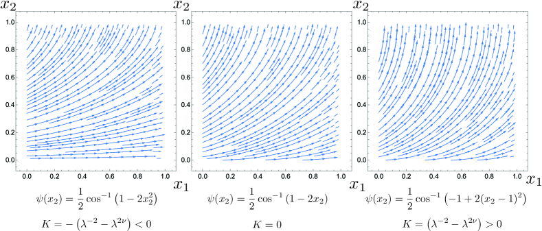
Figure 1: Director fields of the form $\bm{n}=\cos\psi(x_{2})\,\hat{\bm{e}}^{1}+\sin\psi(x_{2})\,\hat{\bm{e}}^{2}$ on the unit square for different choices of the function $\psi=\psi(x_{2})$. The resulting Gaussian curvature $K$ upon stimulation is also indicated.

Director fields of the form (24) can be generated by shifting a fixed curve along the $x_{1}$-axis. We now develop a more geometric description for director fields that can be generated by uniform translation of a curve $\bm{\gamma}=\bm{\gamma}(t)=\gamma_{1}(t)\hat{\bm{e}}^{1}+\gamma_{2}(t)\hat{\bm{e}}^{2}$ along a fixed direction specified by a unit vector $\bm{u}=u_{1}\hat{\bm{e}}^{1}+u_{2}\hat{\bm{e}}^{2}$. For such a director field, it is natural to change coordinates from the Cartesian $(x_{1},x_{2})$ to $(t,r)$ where $t$ is the parameter along the curve $\bm{\gamma}$ and $r$ is the parameter in the direction of translation. That is, we have

$$x_{1}(t,r):=\gamma_{1}(t)+ru_{1},\;\;\;\;\;\;x_{2}(t,r):=\gamma_{2}(t)+ru_{2}.$$ (28)

The director field $\bm{n}=n_{1}\hat{\bm{e}}^{1}+n_{2}\hat{\bm{e}}^{2}$ at each point $(t,r)$ is given by

$$n_{1}(t)=\frac{\gamma_{1}^{\prime}}{\sqrt{\gamma_{1}^{\prime 2}+\gamma_{2}^{\prime 2}}},\;\;\;\;\;\;\;n_{2}(t)=\frac{\gamma_{2}^{\prime}}{\sqrt{\gamma_{1}^{\prime 2}+\gamma_{2}^{\prime 2}}}.$$ (29)

Note that the independence of the director field components from $r$ follows by construction. The metric components $\mathbf{A}=[a_{\alpha\beta}]=\left[(\lambda^{2}-\lambda^{-2\nu})n_{\alpha}n_{\beta}+\lambda^{-2\nu}\delta_{\alpha\beta}\right]$ in Cartesian coordinates transform according to $\mathbf{A}\rightarrow\mathbf{J}^{T}\mathbf{AJ}$, where $\mathbf{J}$ is the Jacobian matrix

$$\mathbf{J}=\left(\begin{array}[]{cc}\partial_{t}x_{1}&\partial_{r}x_{1}\\ \partial_{t}x_{2}&\partial_{r}x_{2}\\ \end{array}\right).$$ (30)

That is,

$$\left(\begin{array}[]{cc}a_{tt}&a_{tr}\\ a_{rt}&a_{rr}\\ \end{array}\right)=\left(\begin{array}[]{cc}\gamma^{\prime}_{1}(t)&u_{1}\\ \gamma^{\prime}_{2}(t)&u_{2}\\ \end{array}\right)^{T}\left(\begin{array}[]{cc}a_{11}&a_{12}\\ a_{21}&a_{22}\\ \end{array}\right)\left(\begin{array}[]{cc}\gamma^{\prime}_{1}(t)&u_{1}\\ \gamma^{\prime}_{2}(t)&u_{2}\\ \end{array}\right)$$ (39)

Now for a given curve $\bm{\gamma}$ and specified direction $\bm{u}$, we can compute the Gaussian curvature as a scalar field $K=K(t)$ using the equation

$$K=-\frac{1}{a_{tt}}\Big{(}\partial_{t}\Gamma^{r}_{tr} -\partial_{r}\Gamma^{r}_{tt}+\Gamma^{t}_{tr}\Gamma^{r}_{tt}$$

$$-\Gamma^{t}_{tt}\Gamma^{r}_{tr}+\Gamma^{r}_{tr}\Gamma^{r}_{tr}-\Gamma^{r}_{tt}\Gamma^{r}_{rr}\Big{)}.$$ (41)

Here we note a remarkable result with an elegant geometric interpretation. Take a circular arc $\bm{\gamma}(t)=R\left(\cos t,\sin t\right)$, where $R=\frac{1}{\sqrt{K}}\left(\lambda^{-2}-\lambda^{2\nu}\right)^{1/2}$, and $K>0$ is a constant. Now let $\bm{u}=(\cos\alpha,\sin\alpha)$, where $\alpha$ is some fixed angle. A direct computation of the Gaussian curvature associated with the director field generated by translating $\bm{\gamma}$ along $\bm{u}$, yields $K$ exactly. It is assumed that the circular arc and direction of translation are chosen such that the director field does not self-intersect.

Recall that the tractrix in the $x_{1}x_{2}$-plane whose axis coincides with the $x_{1}$-axis is the planar curve $\bm{\gamma}$ passing through a point $(0,a)$ with the property that the length of the segment of the tangent line from any point on the curve to the $x_{1}$-axis is constant and equal to $a>0$. One parametric representation of the tractrix is provided by

$$\gamma_{1}(t)=a\,(\tanh t-t),\;\;\;\;\;\;\gamma_{2}(t)=a\,\mathrm{sech}\,t.$$ (42)

We now consider the director pattern that is generated by translating a tractrix along its axis. That is, we take $\bm{\gamma}$ to be as in equation (42) and choose the direction of translation to be $\bm{u}=(1,0)$ as shown in Fig. 2. A direct computation of the Gaussian curvature of such a pattern generated by a tractrix with parameter $a=\frac{1}{\sqrt{|K|}}\left(\lambda^{-2}-\lambda^{2\nu}\right)^{1/2}$ with $K<0$, yields $K$ exactly.

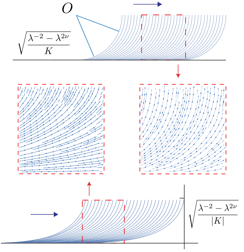
Figure 2: The nematic pattern obtained by shifting a circular arc along a fixed direction generates constant positive Gaussian curvature $K>0$. The nematic pattern obtained by shifting a tractrix along its axis generates constant negative Gaussian curvature $K<0$.

IV Orthogonal Duality

The result that the director fields in Fig. 2 generate opposite Gaussian curvature may seem surprising on first inspection, since the patterns look somewhat similar. However, in light of the orthogonal duality result (23), we find that the patterns make perfect sense. In particular, the positive curvature pattern is equivalent to the pattern obtained by rotating the sheet by $90^{\circ}$. One can see that this equivalent pattern is exactly the orthogonal dual of the negative curvature pattern of Fig. 2, as illustrated in Fig  3.

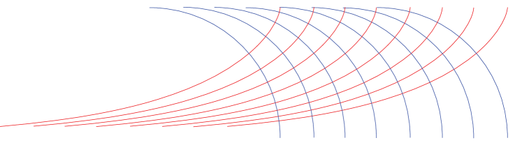
Figure 3: Orthogonal duality of director fields. The director fields that were discovered to generate constant Gaussian curvatures of opposite sign are seen to be equivalent to orthogonally dual patterns. Note that every tractrix intersects every circle at right angles.

This observation is consistent with physical intuition since the mechanical response of nematic solids to stimuli such as heat is a contraction along the director and a simultaneous expansion in the orthogonal directions. Thus, one might expect that the intrinsic curvature properties of a patterned sheet will be qualitatively reversed when the pattern is replaced by its orthogonal dual, even though the scaling factors $\lambda$ and $\lambda^{-\nu}$ are not exact reciprocals when $\nu\neq 1$. Indeed, we have shown that this reversal is exact in the sense that the Gaussian curvature distribution becomes precisely the negative of the dual pattern.

It is also interesting to connect these ideas to the mechanical response of a patterned nematic sheet that is being cooled instead of heated. On cooling an initially flat nematic sheet, the rod-like molecules expand along the director and contract in the orthogonal directions. So once again one may expect the activated surface to exhibit the opposite of the curvature properties that manifest on heating. Quantifying this opposite response however is somewhat delicate, since the scaling coefficients are typically temperature dependent and cooling a flat sheet by a particular temperature will not necessarily produce the exact opposite of the response observed by heating the flat sheet by the same temperature.

V Willmore Functional

It is well known that for a surface in $\mathbb{R}^{3}$, the components $a_{\alpha\beta}$ and $b_{\alpha\beta}$ of the first and second fundamental forms satisfy the Gauss-Codazzi-Mainardi equations

$$\partial_{\beta}\Gamma_{\alpha\sigma\tau}-\partial_{\sigma}\Gamma_{\alpha\beta\tau}+\Gamma^{\mu}_{\alpha\beta}\Gamma_{\sigma\tau\mu}-\Gamma^{\mu}_{\alpha\sigma} \Gamma_{\beta\tau\mu}$$

$$=b_{\alpha\sigma}b_{\beta\tau}-b_{\alpha\beta}b_{\sigma\tau},$$

$$\partial_{\beta}b_{\alpha\sigma}-\partial_{\sigma}b_{\alpha\beta}+\Gamma^{\mu}_{\alpha\sigma}b_{\beta\mu}-\Gamma^{\mu}_{\alpha\beta}b_{\sigma\mu} =0,$$ (43)

where $\Gamma_{\alpha\beta\tau}=\frac{1}{2}(\partial_{\beta}a_{\alpha\tau}+\partial_{\alpha}a_{\beta\tau}-\partial_{\tau}a_{\alpha\beta})$ and $\Gamma^{\sigma}_{\alpha\beta}=a^{\sigma\tau}\Gamma_{\alpha\beta\tau}$. Furthermore, any pair $(a,b)$ consisting of a symmetric and positive definite matrix field $(a_{\alpha\beta})$ and a symmetric matrix field $(b_{\alpha\beta})$ that satisfy the Gauss-Codazzi-Mainardi equations determines a unique surface up to a rigid transformation in $\mathbb{R}^{3}$ Ciarlet (2005).

To determine the equilibrium configuration of the mid-surface of an initially flat nematic sheet upon stimulation, we need to know the components $b_{\alpha\beta}$ of the second fundamental form that minimise the bending energy

$$\mathcal{E}[b]=\frac{1}{3}\int_{\omega}\mathcal{A}^{\alpha\beta\gamma\delta}b_{\alpha\beta}b_{\gamma\delta}\,dS$$ (44)

subject to the Gauss-Codazzi-Mainardi constraints defined by the metric $(a_{\alpha\beta})$ generated by the director field. This functional can be rewritten in terms of the mean and Gaussian curvatures of the mid-surface as

$$\mathcal{E}=\frac{1}{3}\int_{\omega}\left(\frac{4H^{2}}{1-\nu_{\mathrm{el}}}-2K\right)dS.$$ (45)

Since $a_{\alpha\beta}=\bar{a}_{\alpha\beta}$, and the Gaussian curvature $K$ is an isometric invariant, the problem reduces to minimising the Willmore functional

$$I_{W}=\int_{\omega}H^{2}\,dS$$ (46)

among isometric immersions of the metric Efrati et al. (2011); Willmore (2012); Lewicka and Reza Pakzad (2011).

The Willmore functional can be written in terms of the principal curvatures $\kappa_{1}$, $\kappa_{2}$ as

$$I_{W} =\frac{1}{4}\int_{\omega}(\kappa_{1}+\kappa_{2})^{2}dS$$

$$=\frac{1}{4}\int_{\omega}(\kappa_{1}-\kappa_{2})^{2}dS+\int_{\omega}K\,dS,$$ (47)

where $K=\kappa_{1}\kappa_{2}$ is the Gaussian curvature. We note that if the condition $\kappa_{1}=\kappa_{2}$ throughout $\omega$ is consistent with the metric, then the equilibrium configuration corresponding to minimal bending energy is determined by imposing this condition. The sphere is the only compact surface in $\mathbb{R}^{3}$ whose principal curvatures are equal everywhere Willmore (2012). Since surfaces of the same constant Gaussian curvature $K$ are locally isometric by Minding’s theorem Minding (1839), a flat nematic sheet whose director field encodes constant positive curvature $K$ will form part of a sphere of radius $R=1/\sqrt{K}$ upon stimulation, assuming that the sheet is small enough to exclude the possibility of self-intersection as in Fig. 4.

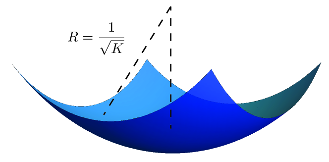
Figure 4: An initially flat nematic sheet forming part of a sphere upon stimulation.

In the case of a thin sheet encoded with constant negative curvature $K<0$, the study of the equilibrium shapes demands a considerably more delicate analysis. We follow Gemmer et al. Gemmer and Venkataramani (2011) and consider equilibrium configurations of hyperbolic elastic disks of radius $R$ that have already undergone local deformations. The equilibrium configurations in the thin sheet limit correspond to minimisers of the Willmore functional or, equivalently, to minimisers of

$$\tilde{I}_{W}=\int_{\omega}\left(\kappa_{1}^{2}+\kappa_{2}^{2}\right)dS,$$ (48)

over isometric immersions of the metric. In geodesic polar coordinates $(\rho,\theta)$, where the metric takes the form $ds^{2}=d\rho^{2}+\left|K\right|^{-1}\sinh^{2}\left(\sqrt{\left|K\right|}\rho\right)d\theta^{2}$, Eq. (48) can be written as

$$\tilde{I}_{W}=\int_{0}^{2\pi}\int_{0}^{R}\;\frac{\sinh\left(\sqrt{\left|K\right|}\rho\right)}{\sqrt{\left|K\right|}}\left(\kappa_{1}^{2}+\kappa_{2}^{2}\right)d\rho\,d\theta.$$ (49)

It is well-known that at every point of a hyperbolic surface, there exists a pair of asymptotic curves along which the normal curvature vanishes Han and Hong (2006). Furthermore, the isometric immersions of the hyperbolic metric of constant Gaussian curvature $K$ are in correspondence with solutions of the sine-Gordon equation:

$$\frac{\partial^{2}\phi}{\partial u\,\partial v}=\left|K\right|\sin\phi(u,v),$$ (50)

where $u$, $v$ are coordinates for a local parametrisation by asymptotic curves and $\phi$ denotes the angle between the asymptotic curves. The angle $\phi$ is related to the principal curvatures by

$$\kappa_{1}^{2}=\left|K\right|\tan^{2}\frac{\phi}{2},\;\;\;\;\;\kappa_{2}^{2}=\left|K\right|\cot^{2}\frac{\phi}{2},$$ (51)

so that

$$\tilde{I}_{W}=\int_{0}^{2\pi}\int_{0}^{R}\;\frac{\sinh\left(\sqrt{\left|K\right|}\rho\right)}{\sqrt{\left|K\right|}}\left(\tan^{2}\frac{\phi}{2}+\cot^{2}\frac{\phi}{2}\right)d\rho\,d\theta.$$ (52)

In Gemmer and Venkataramani (2011), the minimisation of Eq. (52) over all smooth solutions to the sine-Gordon equation is analysed numerically to conclude that the principal curvatures of smooth isometric immersions of a hyperbolic disk of radius $R$ satisfy

$$\max\left(|\kappa_{1}|,|\kappa_{2}|\right)\geq\frac{|K|}{64}e^{2\sqrt{\left|K\right|}R}.$$ (53)

Moreover, it is shown that this lower bound is attained by surfaces that are geodesic disks lying on hyperboloids of revolution of constant Gaussian curvature $K$.

Hyperbolic surfaces whose two asymptotic curves are straight lines that intersect at an angle $\theta$ form a one-parameter family of surfaces $\mathcal{A}_{\theta}$ known as Amsler surfaces Amsler (1955). Each such surface is uniquely determined by the angle $\theta$ between the asymptotic lines. In Gemmer and Venkataramani (2011), the odd periodic extension of a subset of the Amsler surface $\mathcal{A}_{\pi/n}$ bounded between the asymptotic lines is taken to generate a periodic profile with $n$ waves. The resulting $n$-periodic shapes are referred to as periodic Amsler surfaces $A_{n}$, which are not smooth as they have discontinuities in their second derivatives at the lines of inflection.

Numerical investigations of the bending energy associated with geodesic disc cutouts of $A_{n}$ have revealed that for large values of $\epsilon=\sqrt{\left|K\right|}R$, particular $n$-wave periodic Amsler surfaces are energetically more favorable than the smooth saddle shapes that correspond to discs lying on hyperboloids of revolution. Furthermore, it has been shown that there exists a sequence of critical radii $R_{n}\sim\ln(n)$ beyond which the principal curvatures and hence Willmore functional of $A_{n}$ diverge. If the radius of the hyperbolic disc is sufficiently large for periodic Amsler surfaces to be energetically more favorable than the hyperboloid solutions, the particular $n$-wave surface that is expected to form is predicted by identifying the smallest critical radius $R_{n}$ greater than $R$. Thus, as the radius of the hyperbolic disc increases one observes that $n$-periodic shapes with an increasing number of waves become more energetically favorable Gemmer and Venkataramani (2011, 2013).

It is interesting to contrast the case of shape selection of sheets encoded with constant positive curvature with that of sheets patterned with a hyperbolic metric. In the constant positive curvature case, the analysis suggests that subsets of spheres are the most energetically favorable isometric immersions provided that the dimensions of the initial sheet are small enough to rule out self-intersection of the deformed surface. That is, the nature of the solution is not influenced by the shape and size of the initially flat sheet. In the hyperbolic case, however, we notice that the extrinsic geometry of the deformed surface is crucially dependent on the particular shape and size of the initially flat sheet. In particular, surfaces with dramatically different extrinsic geometries may form by simply increasing the size of the sample patterned with a particular intrinsic geometry.

VI Blueprinting nematic sheets of prescribed Gaussian curvature

One can use the shifted circular arc patterns of Fig. 2 to blueprint a metric of constant positive Gaussian curvature that is realised upon stimulation of a thin nematic sheet. Since the magnitude of the Gaussian curvature is determined by the radius of the shifted circular arcs, we need to use a shifted pattern consisting of circular arcs that are $C^{1}$-smoothly joined in order to extend the pattern to cover larger domains, as shown in Fig. 5.

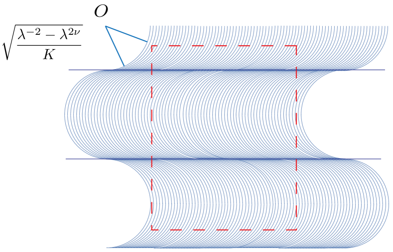
Figure 5: Blueprinting prescribed positive Gaussian curvature $K>0$ on a rectangular sheet of arbitrary dimensions whose edges are indicated by the dashed lines. The Gaussian curvature is well-defined everywhere except along the solid horizontal lines where the distinct arcs join.

The pattern on the larger domain encodes positive Gaussian curvature at all points except along the lines where the distinct circular arcs join. At these points, the Gaussian curvature is not defined and sharp creases may develop upon stimulation. Similarly, one can extend the shifted tractrix patterns of Fig. 2 to encode constant negative curvature on extended domains as shown in Fig. 6. As in the positive curvature case, the Gaussian curvature is not well-defined along the solid horizontal lines indicated in Fig. 6 as the metric components are not continuously differentiable at these points.

In the case of the circular arc patterns, for instance, note that the unit tangents to the arcs give the director field whose first derivative at each point coincides with the vector pointing towards the centre of the circular arc at that point and so clearly exhibits a jump discontinuity across the solid horizontal line. The jump discontinuities of the extended hyperbolic pattern follow by orthogonal duality.

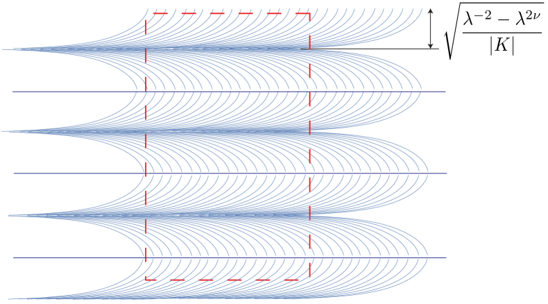
Figure 6: Blueprinting prescribed negative Gaussian curvature $K<0$ on a rectangular sheet of arbitrary dimensions whose edges are indicated by the dashed lines. The Gaussian curvature is well-defined everywhere except along the solid horizontal lines.

VII Nematic patterns on curved surfaces

Often we are interested in shape transitions of surfaces that are initially curved. In such cases the surface may have a non-flat first fundamental form at the outset, which would then change due to the activation of some local deformation pattern. In the context of thin nematic shells, we would start with a shell whose mid-surface is given as an embedding in three dimensions. This embedding determines the first fundamental form as a non-trivial $(0,2)$ metric tensor, which would then change to a new reference metric $\bar{a}_{\alpha\beta}$ that depends on the director field pattern on the surface.

Here we highlight an interesting result on the effect of two sets of director fields on the Gaussian curvature of surfaces of revolution. Consider a surface of revolution whose standard parametrisation is given by

$$\bm{r}(u,v)=\left(f(v)\cos u,f(v)\sin u,g(v)\right),$$ (54)

where the pair of real-valued functions $(f,g)$ specifies the profile curve of the surface. The associated metric is given by

$$ds^{2} =\bm{r}_{u}\cdot\bm{r}_{u}du^{2}+2\bm{r}_{u}\cdot\bm{r}_{v}du\,dv+\bm{r}_{v}\cdot\bm{r}_{v}dv^{2}$$

$$=f^{2}du^{2}+\left(f^{\prime 2}+g^{\prime 2}\right)dv^{2}.$$ (55)

A direct calculation of the Gaussian curvature yields

$$K=\frac{f^{\prime}g^{\prime}g^{\prime\prime}-f^{\prime\prime}g^{\prime 2}}{f(f^{\prime 2}+g^{\prime 2})^{2}}.$$ (56)

Now suppose that the surface is patterned such that the directors are aligned with the $v=\mathrm{constant}$ lines. That is, the director field lines are circles centred on the axis of revolution. The metric upon stimulation becomes

$$ds^{2}=f^{2}\;\lambda^{2}du^{2}+\left(f^{\prime 2}+g^{\prime 2}\right)\;\lambda^{-2\nu}dv^{2},$$ (57)

and the Gaussian curvature transforms as

$$K=\lambda^{2\nu}\frac{f^{\prime}g^{\prime}g^{\prime\prime}-f^{\prime\prime}g^{\prime 2}}{f(f^{\prime 2}+g^{\prime 2})^{2}}.$$ (58)

That is, for any surface of revolution patterned by director fields aligned with the horizontal circles centred on the axis of revolution, the Gaussian curvature transforms according to the elegant formula $K\rightarrow\lambda^{2\nu}K$. This result was established in Modes and Warner (2012) for the special case of a sphere patterned by azimuthal director fields. Here we see that the result is valid for all surfaces of revolution, including surfaces of negative and non-constant Gaussian curvature.

For the orthogonal dual of the considered pattern on any given surface of revolution, the metric upon stimulation is given by

$$ds^{2}=f^{2}\;\lambda^{-2\nu}du^{2}+\left(f^{\prime 2}+g^{\prime 2}\right)\;\lambda^{2}dv^{2},$$ (59)

and a direct calculation of the Gaussian curvature yields

$$K=\lambda^{-2}\frac{f^{\prime}g^{\prime}g^{\prime\prime}-f^{\prime\prime}g^{\prime 2}}{f(f^{\prime 2}+g^{\prime 2})^{2}}.$$ (60)

That is, for any surface of revolution patterned by director fields aligned with the profile curves of the surface (i.e. lines of constant $u$), the Gaussian curvature transforms according to $K\rightarrow\lambda^{-2}K$. Note the remarkable fact that this transformation is independent of the opto-thermal Poisson ratio $\nu$. In the case of a sphere, such patterns correspond to the director fields being aligned with the lines of longitude.

In the special case of a sphere of radius $R$, these results show that upon the stimulation of an azimuthal pattern the Gaussian curvature decreases to $\lambda^{2\nu}/R^{2}$, whereas for the orthogonal dual pattern the Gaussian curvature increases to $\lambda^{-2}/R^{2}$. We now show how these two patterns and the associated Gaussian curvature responses can be viewed as the extreme cases of the family of loxodromic spiral patterns on a sphere, as shown in Fig. 7.

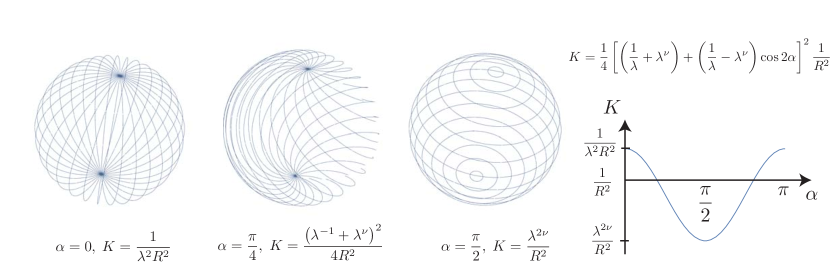
Figure 7: Loxodromic spiral director fields of the form $\bm{n}=\cos\alpha\,\hat{\bm{e}}_{\theta}+\sin\alpha\,\hat{\bm{e}}_{\phi}$ on a sphere of radius $R$ for the cases $\alpha=0,\,\pi/4,\,\pi/2$ and the Gaussian curvature generated upon stimulation. Note that $\alpha$ is the angle that the directors make with the meridian lines.

Recall that a loxodrome on a sphere is the curve that cuts a meridian at a constant angle $\alpha$. If $\alpha$ is not a right angle, then the loxodromes form spirals on the sphere. We assume that a sphere of radius $R$ is patterned with a director field whose integral curves consist of loxodromes of angle $\alpha$, so that $\bm{n}=\cos\alpha\,\hat{\bm{e}}_{\theta}+\sin\alpha\,\hat{\bm{e}}_{\phi}$, where $\theta$ and $\phi$ are the polar and azimuthal angles, respectively, and $\hat{\bm{e}}_{\theta}$, $\hat{\bm{e}}_{\phi}$ are the corresponding unit tangent vectors in $\mathbb{R}^{3}$. Upon stimulation, the point $(\theta,\phi)$ transforms according to $(\theta,\phi)^{T}\rightarrow F(\theta,\phi)^{T}$, where $F$ is the matrix representation of the spontaneous deformation tensor with respect to the orthonormal basis $\hat{\bm{e}}_{\theta}$, $\hat{\bm{e}}_{\phi}$. The round spherical metric $ds^{2}=R^{2}\left(d\theta^{2}+\sin^{2}\theta\,d\phi^{2}\right)$ transforms as

$$ds^{2}\rightarrow\begin{pmatrix}d\theta&d\phi\end{pmatrix}F^{T}a_{0}F\begin{pmatrix}d\theta\\ d\phi\end{pmatrix}=\begin{pmatrix}d\theta&d\phi\end{pmatrix}a\begin{pmatrix}d\theta\\ d\phi\end{pmatrix},$$ (61)

where

$$a_{0}=\begin{pmatrix}R^{2}&0\\ 0&R^{2}\sin^{2}\theta\end{pmatrix}.$$ (62)

Directly computing the Gaussian curvature using the new metric $a=F^{T}a_{0}F$, we obtain the formula

$$K=\frac{1}{4}\left[\left(\frac{1}{\lambda}+\lambda^{\nu}\right)+\left(\frac{1}{\lambda}-\lambda^{\nu}\right)\cos 2\alpha\right]^{2}\frac{1}{R^{2}}.$$ (63)

We notice that the resulting Gaussian curvature is a constant between the values $\lambda^{2\nu}/R^{2}$ and $\lambda^{-2}/R^{2}$ depending on the angle $\alpha$. Note that although the Gaussian curvature upon stimulation is constant and positive in each case, the resulting surface is generally not a sphere. For example, in the case of azimuthal patterns ($\alpha=\pi/2$) a spindle or “thorny sphere” of the corresponding curvature is expected to form Modes and Warner (2012).

VIII Comments

It is often the case that key physical characteristics of materials, such as adhesive and optical properties, are determined by surface structure. The engineering of switchable surfaces consisting of active materials such as nematic glasses offers the possibility of controllably and reversibly changing the surface geometry of thin structures for use in a variety of potential devices. Possible applications may include microfluidic mixers and pumps, adjustable optical lenses and switchable textured surfaces for use in tablet computers. There are two key mechanisms for generating shape transformations in thin sheets of patterned nematic glasses. One method is by means of defects in the director field pattern and the other is by using a smooth in-plane director field that generates Gaussian curvature.

In this paper, we have clearly highlighted smooth director fields that generate constant Gaussian curvature of any desired value, with the hope that such patterns offer feasible initial targets for experimentalists to confirm the predictions of the theory and test its limitations. We have also identified an important symmetry in the Gaussian curvature associated with a given nematic pattern on an initially flat sheet, namely that the orthogonal dual of a given pattern generates the exact opposite Gaussian curvature at every point. This observation has an important practical implication for experimentalists, who can produce a sheet whose Gaussian curvature distribution is the exact opposite of a given patterned sheet by simply adding $\pi/2$ radians to the nematic alignment angle associated with the given sheet. If the viability of producing switchable nematic surfaces using such patterns is confirmed, one may begin to effectively combine more elaborate smooth director fields and topological defects to devise a variety of powerful shaping mechanisms for use in a wide range of potential applications.