Rapidly Evolving and Luminous Transients Driven by Newly Born Neutron Stars

Abstract

We provide a general analysis on the properties of emitting material of some rapidly evolving and luminous transients discovered recently with the Pan-STARRS1 Medium Deep Survey. It is found that these transients are probably produced by a low-mass non-relativistic outflow that is continuously powered by a newly born, rapidly spinning, and highly magnetized neutron star. Such a system could originate from an accretion-induced collapse of a white dwarf or a merger of a neutron star-neutron star binary. Therefore, observations to these transients would be helpful for constraining white dwarf and neutron star physics and/or for searching and identifying gravitational wave signals from the mergers.

1. Introduction

Neutron stars (NSs) are usually born from core collapse of a massive star, during which a luminous supernova can be driven by the intense neutrino emission from the proto-NS by expelling and heating the stellar envelope. Besides this most popular origination, there could be other two ways leading to a NS formation. On one hand, it is believed that, if electron captures in the core can take place more quickly than the nuclear burning, an accreting white dwarf (WD) could collapse into a NS by loosing pressure support rather than lead to a disruption event (e.g. Type Ia supernova; Canal & Schatzman 1976; Nomoto & Kondo 1991). On the other hand, recently it is often suggested that a massive NS could form and survive from a merger of a NS-NS binary (Dai et al. 2006; Fan & Xu 2006; Metzger et al. 2008; Bucciantini et al. 2012; Rowlinson et al. 2010, 2013), during which a highly-beamed relativistic jet can be launched to produce a short-duration gamma-ray burst (GRB; Nakar 2007; Berger 2014). The clues to the post-merger NSs have emerged more and more from the observations of extended emission, X-ray flares, and plateau afterglows of some short GRBs.

During accretion-induced collapses of WDs and NS-NS mergers, a low-mass non-relativistic outflow can be ejected nearly isotropically due to the dynamical centrifugal force and the wind blown from a remnant NS$+$disk system. In such an outflow, some radioactive heavy elements are expected to be synthesized. Then the decay of the elements would generate a faint optical-infrared transient with a duration of several days and a luminosity of $\lesssim 10^{41}\rm erg~{}s^{-1}$ (Darbha et al. 2010; Li & Paczyński 1998; Kulkarni 2005; Rosswog 2005; Metzger et al. 2010; Roberts et al. 2011). In the NS-NS merger case, such transients are now known as kilonovae or macronovae, which have become one of the recent highlights of time domain astronomy since from the observation of the infrared bump after GRB 130603B (Tanvir et al. 2013; Berger et al. 2013).

However, as implied by the X-ray and optical afterglows of GRB 130603B, the GRB jet and thus the isotropic outflow could both be primarily powered by the spin-down of a newly born NS rather than radioactivities (Fan et al. 2013), although its infrared luminosity is still too ambiguous to achieve a definite conclusion. In any case, this observation encouraged us optimistically to consider that the luminosity of the transients during WD collapses and NS-NS mergers could be enhanced significantly by a spinning-down post-collapse/merger NS to be comparable to or even exceed those of ordinary supernova, but still with an obviously short duration due to the low mass of the outflow (Yu et al. 2013; Metzger & Piro 2014). Reasonably, a new class of rapidly evolving and luminous transients were recently reported by Drout et al. (2014) with the Pan-STARRS1 Medium Deep Survey (PS1-MDS), which could therefore be the first smoking-gun observational signatures for the NS-powered transient events during WD collapses and/or NS-NS mergers.

2. The PS1-MDS transients

The PS1-MDS transients were specifically identified by following criteria: the transient must rise by $>$1.5 mag in the 9 days immediately before a peak and decline by $>$1.5 mag in $\sim$25 days after the peak. Such rapid evolution of the transients makes them easily evade from previous supernova surveys until the PS1-MDS which is featured in its rapid cadence and multiple band coverage to a significant depth ($\sim$24 mag). For 10 of the new-discovered PS1-MDS transients, the spectra of their underlying hosts were obtained so that the cosmological redshifts of the transients can be determined to range from $z=0.074$ (PS1-10ah) to $z=0.646$ (PS1-11bbq). Meanwhile, the evolution of the spectral energy distributions of the transients selves was also achieved by interpolating their light curves in five broadband filters ($g_{\rm P1}r_{\rm P1}i_{\rm P1}z_{\rm P1}y_{\rm P1}$). Then, the effective black-body temperatures of the transients (except for PS1-12bb) were revealed to evolve around $20,000$ K, which indicates an ultraviolet emission, near the peak emission time to 7000 K at later times. The pseudo-bolometric luminosities of the transients were correspondingly calculated to have a peak value with the order of $L_{\rm p}\sim 10^{43}\rm erg~{}s^{-1}$. Consequently, the radius of emission region at the peak time can be constrained to be $R_{\rm p}=\left({L_{\rm p}/4\pi\sigma T_{\rm p}^{4}}\right)^{1/2}\sim 3.0\times 10^{14}{\rm cm~{}}L_{\rm p,43}^{1/2}T_{\rm p,4.3}^{-2}$, where $\sigma$ is the Stefan-Boltzmann constant and, hereafter, the conventional notation $Q_{x}=Q/10^{x}$ is adopted in the cgs units.

The above radius, luminosity, and temperature of the PS1-MDS transients indicate that they are probably associated with stellar-size energetic “explosions”. According to the selection criteria of Drout et al. (2014), the peak times $t_{\rm p}$ of the transient light curves can be taken to be from a few to $\sim 10$ days after the explosions. Such short peak times make the transients distinct from the overwhelming majority of ordinary supernovae, which usually reach their peaks after several weeks or a few months from the explosions. More precisely and specifically, the PS1-MDS transients with an intermediate luminosity $<10^{43}\rm erg~{}s^{-1}$ (i.e. PS1-10ah, PS1-10bjp, PS1-12bb, PS1-12brf, PS1- 13dwm, and PS1-13ess) still exhibit some similarities with the previously-reported rare supernova events such as SN 2002bj (Poznanski et al. 2010), SN 2010X (Kasliwal et al. 2010), and SN 2005ek (Drout et al. 2013). However, the completely new luminosity-timescale region opened by the high-luminosity PS1-MDS transients (i.e. PS1- 11qr, PS1-11bbq, PS1-12bv, and PS1-13duy), which has never been probed before, would lead us to consider a completely new branch of stellar explosions.

Regardless of the specific nature of the progenitors of the PS1-MDS transients, a general order-of-magnitude analysis can be made with respect to a cluster of material of mass $M$ and internal energy $E_{\rm int}$ expanding due to its own internal pressure. On one hand, the peak of the material emission generally appears at the time within which photons inside the material can transfer from the core to the outmost surface. By considering of the random walk of the photons, the peak emission time can be expressed by $t_{\rm p}\sim\left({R_{\rm p}/\lambda}\right)^{2}{(\lambda/c)}={3\kappa M/4\pi R_{\rm p}c}$, where $\lambda=(\kappa\rho)^{-1}$ is the average free path, $\kappa$ the opacity, and $\rho$ the density. Then the mass and the kinetic energy of the material can be estimated by

$$M \sim {4\pi R_{\rm p}ct_{\rm p}\over 3\kappa}=0.04~{}{\rm M_{\odot}}~{}\kappa_{-0.3}^{-1}L_{\rm p,43}^{1/2}T_{\rm p,4.3}^{-2}t_{\rm p,6},$$ (1)

and

$$E_{\rm k,p} = {1\over 2}Mv_{\rm p}^{2}\sim 3.3\times 10^{48}{\rm erg}~{}\kappa_{-0.3}^{-1}L_{\rm p,43}^{3/2}T_{\rm p,4.3}^{-6}t_{\rm p,6}^{-1},$$ (2)

respectively, where the expanding velocity is given by

$$v_{\rm p}\sim{R_{\rm p}\over t_{\rm p}}=3.0\times 10^{8}{\rm cm~{}s^{-1}}~{}L_{\rm p,43}^{1/2}T_{\rm p,4.3}^{-2}t_{\rm p,6}^{-1}.$$ (3)

On the other hand, the emission luminosity can be approximatively connected with the internal energy by $L\sim 4\pi RE_{\rm int}c/(3\kappa M)$ by following the diffusion equation $f=({c}/{3\kappa\rho})({\partial u_{\rm int}}/{\partial r})$, where $f=L/(4\pi R^{2})$ is the emission flux, $u_{\rm int}=E_{\rm int}/V$ the internal energy density, and $V={4\over 3}\pi R^{3}$ the volume. Then we get

$$E_{\rm int,p} \sim {3\kappa ML_{\rm p}\over 4\pi R_{\rm p}c}=L_{\rm p}t_{\rm p}=1.0\times 10^{49}{\rm erg~{}}L_{\rm p,43}t_{\rm p,6}.$$ (4)

Together with the equation $4\pi R^{2}p/M=dv/dt\sim v/t$ describing the adiabatic acceleration of the material, the expanding velocity at the peak time can also be calculated by

$${v_{\rm p}} \sim {4\pi R_{\rm p}^{2}p_{\rm p}t_{\rm p}\over M}=4.5\times 10^{8}{\rm cm~{}s^{-1}}~{}\kappa_{-0.3}T_{\rm p,4.3}^{4}t_{\rm p,6},$$ (5)

where the pressure $p={1\over 3}u_{\rm int}$ is adopted. By combining Equations (3) and (5), we can obtain a rough constraint on the opacity as $\kappa\sim 0.7~{}{\rm cm^{2}~{}g^{-1}}~{}L_{\rm p,43}^{1/2}T_{\rm p,4.3}^{-6}t_{\rm p,6}^{-2}$, which indicates an opacity primarily contributed by electron scattering. The above constraint also implies that the basic properties (e.g. mass, expanding velocity, and internal energy) of adiabatically expanding material can be certainly determined with the peak values of its bolometric light curve.

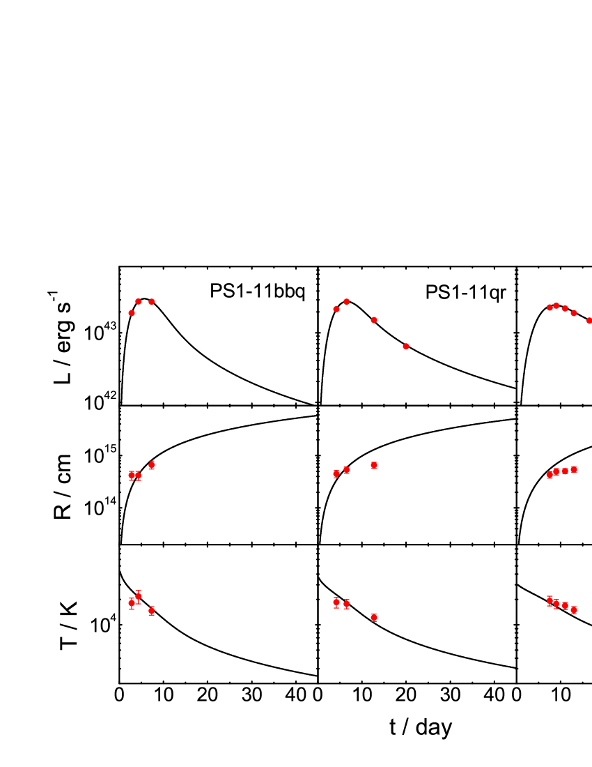
Figure 1.— Comparison between the model-predicted (solid lines) and the observational pseudo-bolometric luminosity, radius, and temperature of the high-luminosity PS1-MDS transients (solid circles). The source PS1-13duy is excluded because only two data points were provided.

3. Energy engine

The mass of the emitting material, which is dramatically smaller than those of ordinary supernova ejecta, suggests that the PS1-MDS transients probably involve an explosion of a system governed by an extremely-stripped star or, more probably, stellar-size compact objects. The material ejected during the explosion could be heated by the energy engine “impulsively” or by some other energy sources after the explosion.

First of all, as a conventional consideration, the emitting material could be impulsively heated by a shock and therefore the emission luminosity is determined by the shock breakout radius. However, owing to a limit on the radius of the largest red supergiant (Levesque et al. 2009), only the PS1-MDS transients with an intermediate luminosity $<10^{43}\rm erg~{}s^{-1}$ can possibly be attributed to a shock breakout from a normal star. For the high-luminosity ones (i.e. PS1- 11qr, PS1-11bbq, PS1-12bv, and PS1-13duy), Drout et al. (2014) suggested that these transients could be associated with a shock breakout within a dense stellar wind. In this case, however, an unexpected high mass-loss rate and an ad hoc mass-loss history of the progenitor need to be invoked. Then, Kashiyama & Quataert (2015) proposed that the impulsive heating could be accomplished in a very hot super-Eddington fall-back accretion disk surrounding a newly born black hole, where a low-mass outflow can be driven by the disk radiation pressure. Such a model can work if the collapsing progenitor star is elaborately designed to eject a just-right mass of material so that a successful supernova can be avoided but an appropriate fall-back accretion disk can still be maintained.

Table 1Parameters for fittings to the light curves

Events	$M/\rm 10^{-2}M_{\odot}$	$\xi L_{\rm sd,i}/10^{44}\rm erg~{}s^{-1}$	$t_{\rm sd}/\rm day$
PS1 - 11bbq	2.0	4.5	2.0
PS1 - 11qr	1.5	1.5	5.0
PS1 - 12bv	1.5	0.65	14

In contrast, a post-explosion energy supply could be a more natural and attractive choice, which can be provided by radioactive decay of heavy elements and/or a long-lasting energy engine. In the radioactivity scenario, the mass of heavy elements represented by ${}^{56}\rm Ni$ is required to be $M_{\rm Ni}\sim m_{\rm Ni}{E_{\rm int,p}/(q_{\rm Ni}+q_{\rm Co})}\sim 0.05~{}{\rm M_{\odot}}L_{\rm p,43}t_{\rm p,6}$, where $m_{\rm Ni}$ is the mass of a ⁵⁶Ni atom and $q_{\rm Ni}=$1.78 MeV and $q_{\rm Co}=$3.505 MeV are the energy release for the decay of per ⁵⁶Ni and per subsequent ⁵⁶Co, respectively. As shown, for a sufficiently high luminosity, the required nickel mass could unrealistically exceed the total mass of the emitting material. Even for a relatively low luminosity, an unacceptable high nickel fraction is also predicted, because the nickel mass is only slightly lower than the total mass. Therefore, the radioactivity must not be the primary energy source for the PS1-MDS transients and alternatively a long-lasting energy engine becomes necessary and crucial. The long activity of the engine further requires that the post-explosion compact object should be a NS rather than a black hole, as previously suggested for GRBs (Dai & Lu 1998a,b; Zhang & Mészáros 2001) and superluminous supernovae (Kasen & Bildsten 2010). The energy that a NS can provide to power the explosion outflow mainly comes from its spin-down with a luminosity $L_{\rm sd}(t)=L_{\rm sd,i}\left(1+{t}/{t_{\rm sd}}\right)^{-2}$. Then by taking appropriate values of the parameters $M$, $L_{\rm sd,i}$ and $t_{\rm sd}$ as listed in Table 1, we employ a semi-analytical light curve model (see Appendix for details) to account for the pseudo-bolometric light curves of the high-luminosity PS1-MDS transients (i.e., PS1-11qr, PS1-11bbq, and PS1-12bv) as well as the evolution of radius and temperature of the transients, as presented in Figure 1. In our fittings, a typical constant opacity $\kappa=0.5\rm cm^{2}g^{-1}$ is artificially adopted to reduce the parameter freedom and an uncertain parameter $\xi$ is introduced to represent the energy injection efficiency.

Being represented by the braking mechanism due to magnetic dipole radiation, the spin-down luminosity and timescale of a NS can be expressed by $L_{\rm sd,i}=10^{7}{\rm~{}erg~{}s^{-1}}~{}B^{2}P_{\rm i}^{-4}$ and $t_{\rm sd}=2\times 10^{39}{\rm s}~{}B^{-2}P_{\rm i}^{2}$, where $B$ and $P_{\rm i}$ are the magnetic field strength and initial spin period, respectively. Then, from the fitting parameters, the values of $B$ and $P_{\rm i}$ can be derived as functions of the parameter $\xi$, as presented in Table 2. It is shown that the involved NSs should be highly magnetized and spin rapidly with a millisecond period, in spite of the uncertainty of the energy injection efficiency. In short, the PS1-MDS transients (at least the high-luminosity ones) are probably produced by a low-mass outflow that is continuously powered by a millisecond magnetar. Specifically, such a newly born NS could originate from an accretion-induced collapse of a WD or a merger of a NS-NS binary. During these processes, a strong magnetic field can be naturally generated and amplified via flux freezing and dynamo action (Duncan & Thompson 1992; Cheng & Yu 2014). On the contrary, for an extremely-stripped star, it is nearly impossible to produce a millisecond magnetar through its collapse.

Table 2Neutron star parameters

Events	$P_{\rm i}/\rm ms$	$B/10^{14}\rm G$
PS1 - 11bbq	16$\xi^{1/2}$	17$\xi^{1/2}$
PS1 - 11qr	18$\xi^{1/2}$	12$\xi^{1/2}$
PS1 - 12bv	16$\xi^{1/2}$	6.5$\xi^{1/2}$

4. Discussions

In view of the high similarity in the post-explosion configurations between the WD collapses and NS-NS mergers, it is not easy to clearly discriminate these two models by the present observations of the PS1-MDS transients.

Firstly, the derived spin periods of $\sim 16-18$ ms for $\xi\sim 1$ seems only prohibited by WD collapses but conflict with NS-NS mergers, because the high initial angular momentum of the binary would give a limiting spin period of $P_{\rm i}\sim 1$ ms to the post-merger NSs. However, in fact, it is widely believed that such a near-Keplerian spinning NS would lose its rotational energy immediately by radiating gravitational waves (Dall’Osso et al. 2015), amplifying magnetic fields (Cheng & Yu 2014), and producing short GRBs and subsequent extended emission (Metzger et al. 2008; Bucciantini et al. 2012). As a result, the initial period for magnetic dipole radiation would become much longer than $\sim 1$ ms, e.g., $P_{\rm i}=5$ ms (e.g. Cheng & Yu 2014). For such a reference value, we can constrain the energy injection efficiency to be $\xi\sim 10$%. This might be caused by that (1) the majority of the spin-down luminosity is concentrated into the GRB direction to contribute a plateau afterglow emission (Yu et al. 2010), which however probably deviates from the light of sight and, perhaps, (2) the spin-down luminosity on the light of sight could also be partly released through X-ray emission by the NS wind itself (Dai 2004; Metzger & Piro 2014). Therefore, such wind X-ray emission associated with the UV-optical transients, if exists, could provide a testable signal for our model.

Secondly, the NS-NS merger model is seemingly challenged by other two issues. (1) As pointed out by Drout et al. (2014), the explosion site offsets of all transients with respect to their host galaxies are statistically smaller than those expected for NS-NS mergers. (2) As calculated by Kasen et al. (2013), the opacity of the neutron-rich outflow could be on the order of magnitude of $10-100\rm cm^{2}~{}g^{-1}$ due to the synthesization of lanthanides, which is much higher than the opacity inferred here. However, on one hand, if we individually pick up the offsets of the high-luminosity transients, we will find that most of them are actually on the high side of the offset distribution. On the other hand, the opacity of the outflow actually can be reduced by two effects: (1) the lanthanide synthesization in the disk wind component of the outflow is blocked due to the neutrino irradiation from the post-merger NS (Metzger & Fernández 2014) and (2) the lanthanides in the dynamical component of the outflow could be ionized by the X-ray emission from the NS wind (Metzger & Piro 2014).

Finally, a potential discrimination between the two models may arise from the explanation of the event rate of PS1-MDS transients, i.e., roughly, $\sim 3200\rm Gpc^{-3}yr^{-1}$ corresponding to the four high-luminosity transients. As a comparison, the rate of Type Ia supernovae was found to $(3.01\pm 0.062)\times 10^{4}\rm Gpc^{-3}yr^{-1}$ from the Lick Observatory Supernova Search (Li et al. 2011) and the rate of NS-NS mergers is also widely considered to be on the order of $\sim 1000\rm Gpc^{-3}yr^{-1}$ (Kalogera et al. 2004). Therefore, optimistically, the event rate of PS1-MDS transients could in principle be accounted for in both the WD collapse and NS-NS merger models, as long as a remarkable fraction of these processes can lead to a NS formation. The rationality of such fractions could be tested by some further model implications, e.g., the cosmic fraction of neutron-rich elements, the detectability of associated gravitational wave signals by Advanced LIGO and Virgo (Abadie et al. 2010; Nissanke et al. 2013), and the detectability of subsequent radio transients arising from the interaction between the outflow and circum medium (Metzger et al. 2015), etc. For this purpose, some detailed calculations and simulations need to be implemented with the constraints derived in this Letter.

5. Conclusion

The luminosity-timescale region opened by the PS1-MDS transients, which although could be partly overlapped by the shock breakout emission of some supernovae, leads us to get a glimpse of a completely new branch of stellar-size explosion phenomena. The mass and energy requirements on the emitting material for the transients robustly indicate a post-explosion system consisting of a newly born millisecond magnetar and a low-mass non-relativistic isotropic outflow. Such a system could originate from accretion-induced collapses of WDs or mergers of NS-NS binaries. Therefore, future observations to these transients would play a vital role in constraining WD and NS physics and/or in searching and identifying gravitational wave radiation.

Appendix A The light curve model

Following Arnett (1980) and Kasen & Bildsten (2010), a semi-analytical light curve model for NS-powered mergernovae was provided by Yu et al. (2013), where relativistic effects were taken into account. Here, in view of the non-relativistic velocity inferred from the PS1-MDS transients, we alternatively adopt a simplified non-relativistic version of the model, which was previously described in detail by Kasen & Bildsten (2010) for superluminous supernovae. In this case, the dynamical evolution of an outflow can be determined by

$${dv\over dt}={4\pi R^{2}p\over M}$$ (A1)

and

$${dR\over dt}=v,$$ (A2)

where the pressure $p={1\over 3}(u_{\rm int}-u_{\rm e})$ with $u_{\rm int}$ being the internal energy density and $u_{\rm e}$ being the energy density releasing by emission. With an energy supply rate $\xi L_{\rm sd}$, the evolution of the outflow internal energy is determined by the energy conservation law as

$$\frac{dE_{\rm int}}{dt}=\xi L_{\rm sd}-L-p\frac{dV}{dt},$$ (A3)

where $L$ is the emission luminosity and the work $-pdV=-4\pi R^{2}pv$ represents the energy loss due to the expansion of the outflow. The emission luminosity can further be related to the internal energy by $L={E_{\rm int}c/(\tau R)}$ for $t\leq t_{\tau}$ and $L={E_{\rm int}c/R}$ for $t>t_{\tau}$, where $\tau=3\kappa M/4\pi R^{2}$ is the optical depth and the time $t_{\tau}$ represents the time for the optical thick-thin transition. Then, by setting the parameters $\kappa$, $M$, $\xi L_{\rm sd,i}$, and $t_{\rm sd}$, a light curve can be solved from the above equations. Three typical types of light curves are presented in Figure 2.

For an analytical understanding of the light curve profiles, we can approximate the spin-down power of the NS by a broken-power-law function as

$$L_{\rm sd} = \xi L_{\rm d,i},{\rm~{}~{}~{}~{}~{}~{}~{}~{}~{}~{}~{}~{}~{}~{}~{}~{}~{}for~{}}t<t_{\rm sd},$$ (A4)

$$= \xi L_{\rm d,i}(t/t_{\rm sd})^{-2},{\rm~{}~{}~{}for~{}~{}~{}}t>t_{\rm sd}.$$ (A5)

Meanwhile, by introducing the photon diffusion time of $t_{\rm d}=(3\kappa M/4\pi vc)^{1/2}$ with a constant velocity, Equation (A3) can be rewritten to (Kasen & Bildsten 2010)

$${dE_{\rm int}t\over dt}={\dot{E}_{\rm supl}t_{\rm d}^{2}-E_{\rm int}t\over t_{\rm d}^{2}}t$$ (A6)

for $t<t_{\tau}$. The shape of light curves mainly depends on the relation between the timescales $t_{\rm d}$ and $t_{\rm sd}$. Let us consider the case of $t_{\rm sd}<t_{\rm d}$ as an example. Firstly, for $t<t_{\rm sd}$, the energy supply is constant and the solution of Eq. (A6) can be derived to

$$L={E_{\rm int}t\over t_{\rm d}^{2}}=\xi L_{\rm d,i}\left(1-e^{-t^{2}/2t_{\rm d}^{2}}\right)\approx\xi L_{\rm d,i}\left({t^{2}\over 2t_{\rm d}^{2}}\right).$$ (A7)

Secondly, for $t_{\rm sd}<t<t_{\rm d}$, by omitting the minor important radiation effect and simplifying Eq. (A6) to ${d(E_{\rm int}t)/dt}\approx{\xi L_{\rm d,i}t_{\rm sd}^{2}/t}$, we can get

$$L \approx \xi L_{\rm d,i}\left(1-e^{-{t_{\rm sd}^{2}/2t_{\rm d}^{2}}}\right)+{\xi L_{\rm d,i}t_{\rm sd}^{2}\over t_{\rm d}^{2}}\ln{t\over t_{\rm sd}}$$ (A8)

$$\approx {\xi L_{\rm d,i}t_{\rm sd}^{2}\over t_{\rm d}^{2}}\left({1\over 2}+\ln{t\over t_{\rm sd}}\right).$$

Thirdly, for $t>t_{\rm d}$, the radiation term becomes dominative in Eq. (A6), i.e., ${d(E_{\rm int}t)/dt}\approx-{E_{\rm int}t^{2}/t_{\rm d}^{2}}$, which gives

$$L \approx \left[\xi L_{\rm d,i}\left(1-e^{-{t_{\rm sd}^{2}/2t_{\rm d}^{2}}}\right)+{\xi L_{\rm d,i}t_{\rm sd}^{2}\over t_{\rm d}^{2}}\ln{t_{\rm d}\over t_{\rm sd}}\right]e^{-{(t^{2}-t_{\rm d}^{2})\over 2t_{\rm d}^{2}}}$$ (A9)

$$\approx {\xi L_{\rm d,i}t_{\rm sd}^{2}\over t_{\rm d}^{2}}\left({1\over 2}+\ln{t_{\rm d}\over t_{\rm sd}}\right)e^{-{(t^{2}-t_{\rm d}^{2})\over 2t_{\rm d}^{2}}}.$$

Finally, as the emission luminosity deceases to approach the energy supply luminosity, the succeeding evolution of the emission luminosity should track the evolution of the energy supply (i.e., $L\propto t^{-2}$), because after $t_{\rm d}$ the freshly deposited internal energy can escape from the outflow nearly immediately. The above treatment can be easily extended to the other two cases of $t_{\rm sd}\sim t_{\rm d}$ and $t_{\rm sd}>t_{\rm d}$. Then a completed solution to Eq. (A6) can be summarized as follows:

Case I: For $t_{\rm sd}<t_{\rm d}$

$$L\propto\left\{\begin{array}[]{ll}t^{2},&{~{}\rm for~{}}t<t_{\rm sd},\\ \ln t,&{~{}\rm for~{}}t_{\rm sd}<t<t_{\rm d},\\ e^{-t^{2}},&{~{}\rm for~{}}t_{\rm d}<t<t_{\rm c},\\ t^{-2},&{~{}\rm for~{}}t>t_{\rm c},\end{array}\right.$$ (A10)

Case II: For $t_{\rm sd}\sim t_{\rm d}$

$$L\propto\left\{\begin{array}[]{ll}t^{2},&{~{}\rm for~{}}t<t_{\rm sd},\\ t^{-2},&{~{}\rm for~{}}t>t_{\rm sd},\end{array}\right.$$ (A11)

Case III: For $t_{\rm sd}>t_{\rm d}$

$$L\propto\left\{\begin{array}[]{ll}t^{2},&{~{}\rm for~{}}t<t_{\rm d},\\ t^{0},&{~{}\rm for~{}}t_{\rm d}<t<t_{\rm sd},\\ t^{-2},&{~{}\rm for~{}}t>t_{\rm sd},\end{array}\right.$$ (A12)

where $t_{\rm c}$ is defined as the time at which $L\rightarrow\xi L_{\rm sd}$. The above three different solutions just correspond to the three types of light curves presented in Figure 2. In all cases, the peak luminosity of the emission appears at the diffusion time $t_{\rm d}$. The three high-luminosity PS1-MDS transients are all fitted by the model with $t_{\rm sd}\sim t_{\rm d}$ in the text.

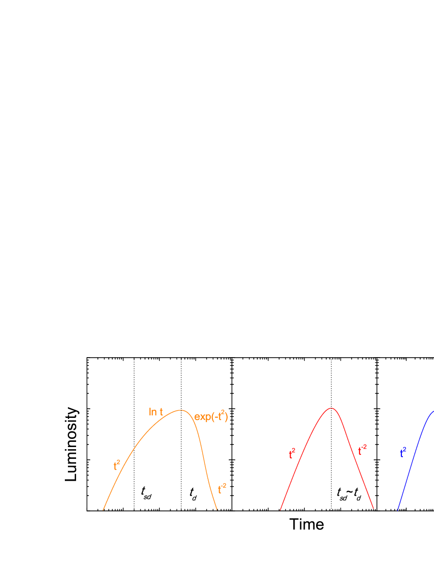
Figure 2.— Three typical types of light curves, where the approximative temporal behaviors are labeled for different evolution phases.

References

- (1) Abadie, J., et al. 2010, Classical and Quantum Gravity, 27, 173001
- (2) Arnett, W. D. 1980, ApJ, 237, 541
- (3) Berger, E., Fong, W., & Chornock, R. 2013, ApJ, 774, L23
- (4) Berger, E. 2014, ARA&A, 52, 43
- (5) Bucciantini, N., Metzger,B. D., Thompson,T. A., & Quataert, E. 2012, MNRAS, 419, 1537
- (6) Canal, R., & Schatzman, E. 1976, A&A, 46, 229
- (7) Cheng, Q., & Yu, Y.-W. 2014, ApJ, 786, L13
- (8) Dai, Z. G. 2004, ApJ, 606, 1000
- (9) Dai, Z. G., & Lu, T. 1998a, Phys. Rev. Lett., 81, 4301
- (10) Dai, Z. G., & Lu, T. 1998b, A&A, 333, L87
- (11) Dai, Z. G., Wang, X. Y., Wu, X. F., & Zhang, B. 2006, Science, 311, 1127
- (12) Dall’Osso, S., Giacomazzo, B., Perna, R., Stella, L. 2015, ApJ, 798, 25
- (13) Darbha, S., et al. 2010, MNRAS, 409, 846
- (14) Drout, M. R., et al. 2013, ApJ, 774, 58
- (15) Drout, M. R., et al. 2014, ApJ, 794, 23
- (16) Duncan, R. C., & Thompson, C. 1992, ApJ, 392, L9
- (17) Fan, Y.-Z., & Xu, D. 2006, MNRAS, 372, L19
- (18) Fan, Y.-Z., Yu, Y.-W., Xu, D., Jin, Z.-P., Wu, X.-F., Wei, D.-M., Zhang, B. 2013, ApJ, 779, L25
- (19) Kalogera, V., et al. 2004, ApJ, 601, L179
- (20) Kasen, D., & Bildsten, L. 2010, ApJ, 717, 245
- (21) Kasen, D., Badnell, N. R., & Barnes, J. 2013, ApJ, 774, 25
- (22) Kashiyama, K., & Quataert, E. 2015, arXiv:1504.05582
- (23) Kasliwal, M. M., et al. 2010, ApJ, 723, L98
- (24) Kulkarni, S. R. 2005, arXiv:astro-ph/0510256
- (25) Levesque, E. M., Massey, P., Plez, B., & Olsen, K. A. G. 2009, AJ, 137, 4744
- (26) Li, L.-X., & Paczyński, B. 1998, ApJ, 507, L59
- (27) Li, W., et al. 2011, MNRAS, 412, 1473
- (28) Metzger, B. D., Quataert, E., Thompson, T. A. 2008, MNRAS, 385, 1455
- (29) Metzger, B. D., Piro, A. L., & Quataert, E. 2009, MNRAS, 396, 304
- (30) Metzger, B. D., et al. 2010, MNRAS, 406, 2650
- (31) Metzger, B. D., & Fernández, R. 2014, MNRAS, 441, 3444
- (32) Metzger, B. D., & Piro, A. L. 2014, MNRAS, 439, 3916
- (33) Metzger, B. D., Williams, P. K. G.. Berger, E. eprint arXiv: 1502.01350
- (34) Nakar, E. 2007, Phys. Rep., 442, 166
- (35) Nissanke, S., Kasliwal, M., & Georgieva, A. 2013, ApJ, 767, 124
- (36) Nomoto, K., & Kondo, Y. 1991, ApJ, 367, L19
- (37) Poznanski, D., et al. 2010, Science, 327, 58
- (38) Roberts, L. F., Kasen, D., Lee, W. H., & Ramirez-Ruiz, E. 2011,ApJ, 736, L21
- (39) Rosswog, S. 2005, ApJ, 634, 1202
- (40) Rowlinson, A., O’Brien, P. T., Tanvir, N. R., et al. 2010, MNRAS, 409, 531
- (41) Rowlinson, A., O’Brien, P. T., Metzger, B. D., Tanvir, N. R., & Levan, A. J. 2013, MNRAS, 430, 1061
- (42) Tanvir, N. R., et al. 2013, Nature, 500, 547 ApJ, 746, 180
- (43) Yu, Y. W., Cheng, K. S., & Cao, X. F. 2010, ApJ, 715, 477
- (44) Yu, Y.-W., Zhang, B., & Gao, H. 2013, ApJ, 776, L40
- (45) Zhang, B., & Mészáros, P. 2001, ApJ, 552, L35