Deep NuSTAR and Swift Monitoring Observations of the Magnetar 1E 1841$-$045

Abstract

We report on a 350-ks NuSTAR observation of the magnetar 1E 1841$-$045 taken in 2013 September. During the observation, NuSTAR detected six bursts of short duration, with $T_{\rm 90}\stackrel{{\scriptstyle<}}{{{}_{\sim}}}1\rm\ s$. An elevated level of emission tail is detected after the brightest burst, persisting for $\sim$1 ks. The emission showed a power-law decay with a temporal index of 0.5 before returning to the persistent emission level. The long observation also provided detailed phase-resolved spectra of the persistent X-ray emission of the source. By comparing the persistent spectrum with that previously reported, we find that the source hard-band emission has been stable over approximately 10 years. The persistent hard X-ray emission is well fitted by a coronal outflow model, where $e^{\pm}$ pairs in the magnetosphere upscatter thermal X-rays. Our fit of phase-resolved spectra allowed us to estimate the angle between the rotational and magnetic dipole axes of the magnetar, $\alpha_{\rm mag}=0.25$, the twisted magnetic flux, $2.5\times 10^{26}\rm\ G\ cm^{2}$, and the power released in the twisted magnetosphere, $L_{j}=6\times 10^{36}\rm\ erg\ s^{-1}$. Assuming this model for the hard X-ray spectrum, the soft X-ray component is well fit by a two-blackbody model, with the hotter blackbody consistent with the footprint of the twisted magnetic field lines on the star. We also report on the 3-year Swift monitoring observations obtained since 2011 July. The soft X-ray spectrum remained stable during this period, and the timing behavior was noisy, with large timing residuals.

1. Introduction

Magnetars are neutron stars to have emission that is powered by the decay of their intense magnetic fields (Duncan & Thompson, 1992; Thompson & Duncan, 1996). The magnetic field strengths inferred from the spin-down parameters are typically greater than $10^{14}\rm\ G$ (e.g., Vasisht & Gotthelf, 1997; Kouveliotou et al., 1998), though there are several sources with lower inferred field strengths (e.g., SGR 0418$+$5729, Swift J1822.3$-$1606; Rea et al., 2010; Scholz Kaspi & Cumming, 2014). There are 28 magnetars discovered to date, including six candidates (see Olausen & Kaspi, 2014).

Short X-ray bursts are often detected from magnetars. The bursts have a variety of morphologies, spectra, and energies, and are thought to be produced by crustal or magnetospheric activity (Thompson et al., 2002). Interestingly, some bursts are followed by a long emission tail while others are not. It has been suggested that the energy in the burst and the integrated energy in the burst tail are correlated (for SGR 1900$+$14 and SGR 1806$-$20, Lenters et al., 2003; Göğüş et al., 2011), which may imply that their relative strengths show a narrow distribution. Woods et al. (2005) suggested a bimodal distribution for the relative strengths across magnetars, implying two distinct physical mechanisms for the bursts. In addition to short X-ray bursts, giant flares and dramatic increases in the persistent emission over days to months have been also observed in some sources (see Woods & Thompson, 2006; Kaspi, 2007; Rea & Esposito, 2011; Mereghetti, 2013, for reviews).

The persistent emission of magnetars in the X-ray band below $\sim$10 keV is dominated by thermal emission and is often modeled with two blackbodies from two hot regions on the surface, or with a surface blackbody plus a power law resulting from magnetospheric reprocessing (Thompson et al., 2002; Zane et al., 2009). Some magnetars also show significant emission in the hard X-ray band above $\sim$10 keV (Kuiper et al., 2006) which is believed to be produced in the magnetosphere (Thompson & Beloborodov, 2005; Heyl & Hernquist, 2005; Baring & Harding, 2007; Beloborodov & Thompson, 2007). Recently, Beloborodov (2013) proposed a coronal outflow model for the hard X-ray emission. The model makes specific predictions for phase-resolved spectra which can be tested by observations. It has been applied to four magnetars with available phase-resolved data above 10 keV, and in all cases the model was found consistent with the data (An et al., 2013; Hascoët, Beloborodov & den Hartog, 2014; Vogel et al., 2014).

The magnetar 1E 1841$-$045 has a surface dipolar magnetic-field strength of $B\equiv 3.2\times 10^{19}(P\dot{P})^{1/2}\ \rm\ G=6.9\times 10^{14}\rm\ G$, estimated from the spin period and the spin-down rate of $P=11.8$ s and $\dot{P}=4\times 10^{-11}\rm\ s\ s^{-1}$, respectively, assuming the standard vacuum dipole spin-down model. The source has previously shown occasional X-ray bursts with energies of $\sim 10^{38}\rm\ erg$ assuming a distance of 8.5 kpc (Kumar & Safi-Harb, 2010; Lin et al., 2011; Dib & Kaspi, 2014). No tails or significant enhancement in the persistent emission were observed following the bursts. Kumar & Safi-Harb (2010) reported detection of emission lines $\stackrel{{\scriptstyle>}}{{{}_{\sim}}}$20 keV in the burst spectrum measured with the Swift Burst Alert Telescope (BAT). Furthermore, the authors argued that the source brightened, and the emission became softer after the burst activity. However, Lin et al. (2011) did not find any emission line, flux enhancement or spectral changes at the burst epoch, in contradiction with the results of Kumar & Safi-Harb (2010).

1E 1841$-$045 is one of the brightest magnetars in the hard X-ray band above 10 keV. Its persistent emission has been studied by Kuiper et al. (2006) and An et al. (2013). The measured photon index in the hard X-ray band is $\Gamma\sim 1.3$, and the pulsed fraction was reported to increase with photon energy. An et al. (2013) applied the coronal outflow model of Beloborodov (2013) to a 50-ks NuSTAR observation and constrained the hard X-ray emission geometry to two possible solutions. Furthermore, an interesting feature was found in the pulse profile in the 24–35 keV band, which may be associated with a spectral feature in this band.

In this paper, we further investigate the properties of persistent emission of 1E 1841$-$045 using a new 350-ks NuSTAR observation and 3-year monitoring observations by Swift. Fortuitously, the source was actively bursting during the NuSTAR observation, which provided an opportunity to study the bursts in addition to the persistent emission. We describe the NuSTAR and archival Chandra, XMM-Newtor and Swift observations used in this paper in Section 2 and present the results of the NuSTAR data analysis in Section 3. We then present the Swift monitoring observations and the data analysis in Sections 4 and 4.1. We discuss the results of data analyses in Section 5 and summarize our main conclusions in Section 6.

Table 1Summary of observations used in this work

Observatory	Obs. ID	Obs. Date	Exposure	Mode
		(MJD)	(ks)
Chandra	730	51754.3	10.5	CC
XMM-Newton	0013340101	52552.2	3.9	FW/LW
XMM-Newton	0013340102	52554.2	4.4	FW/LW
Chandra	6732	53946.4	24.9	TE
Swift	00080220003	56241.3	17.9	PC
Swift	00031863050	56551.3	4.3	WT
Swift	00080220004	56556.5	1.9	PC
NuSTAR	30001025002	56240.9	48.6	$\cdots$
NuSTAR	30001025004	56540.3	35.9	$\cdots$
NuSTAR	30001025006	56542.4	77.9	$\cdots$
NuSTAR	30001025008	56547.1	85.7	$\cdots$
NuSTAR	30001025010	56549.6	53.3	$\cdots$
NuSTAR	30001025012	56556.5	100.7	$\cdots$

^aCC: Continuous Clocking, FW: Full Window, LW: Large Window, PC: Photon Counting, TE: Timed Exposure, WT: Windowed Timing. MOS1,2/PN for XMM-Newton.
^bSwift observations used for spectral analysis in Section 3.2.3. Results of analysis on a larger Swift monitoring dataset are presented in Section 4.

2. Observations

1E 1841$-$045 was observed with NuSTAR (Harrison et al., 2013) between 2013 September 5 and 21 in a series of exposures with durations 40–100 ks with a total net exposure of 350 ks. Two X-ray bursts were detected with the Fermi Gamma-Ray Burst Monitor (GBM) (Collazzi, Xiong, & Kouveliotou, 2014; Pal’shin et al., 2014) on 2013 September 13, during the NuSTAR observation period. Fortunately, the bursts were also recorded in the NuSTAR data. In addition to the Fermi reported bursts, NuSTAR serendipitously detected several more bursts. We report on the bursts in Section 3.1. To study the persistent emission of the source, we also analyzed archival observations made previously with NuSTAR, Chandra, XMM-Newton and Swift to have better statistics and to constrain the persistent properties of the source in the soft band. The observations used in this study are listed in Table 1. Note that all the soft-band observations and the first NuSTAR observation (Obs. ID 30001025002) were reported previously (An et al., 2013, A13 hereafter).

The NuSTAR data were processed with nupipeline 1.3.1 along with CALDB version 20131223. We used default filters except for PSDCAL for which we used PSDCAL=NO. The PSDCAL filter is for laser metrology calibration of the relative positions of the optics and detectors. This observation was affected by times when the metrology laser went out of range. By not using the default, the pointing accuracy may be slightly degraded, but good time intervals (GTI), and hence exposure time, increase. We note this situation is unusual and specific to this observation. We verified that the analysis results described below do not change depending on the PSDCAL filter setting. However, we note that some of the burst data could be retrieved only with PSDCAL=NO.

We also analyzed archival XMM-Newton and Chandra observations (see Table 1). The XMM-Newton data were processed with Science Analysis System (SAS) 12.0.1, and the Chandra data were reprocessed using chandra_repro of CIAO 4.4 along with CALDB 4.5.3. We further processed the cleaned data for analysis as described below. Uncertainties below are at the 1$\sigma$ confidence level unless stated otherwise.

3. Data Analysis and Results for the NuSTAR observations

In this Section, we present data analysis results for bursts and persistent emission measured with the observations in Table 1 (Sections 3.1-3.3). We fit the persistent and phase-resolved spectra with the coronal outflow model and show the results in Section 3.4.

3.1. Burst Analysis

3.1.1 Temporal and Spectral Properties of the Bursts

Table 2Deadtime-corrected Properties of NuSTAR-detected Bursts from 1E 1841$-$045

Burst	$T_{\rm 0}$	$\phi$	$T_{\rm r}$	$T_{\rm f}$	$A$	$C_{\rm 1}$	$C_{\rm 2}$	$T_{\rm 90}$	$N_{\rm evt}$	$\Delta_{\rm post-pre}$
	(day)		(s)	(s)	(cps)	(cps)	(cps)	(s)	(cts)	(cts)
1	0.35836545	$0.2266^{+0.0003}_{-0.0002}$	$0.007^{+0.001}_{-0.001}$	$0.047^{+0.017}_{-0.019}$	$1740^{+760}_{-600}$	$12^{+2}_{-2}$	$<16$	$0.12^{+0.04}_{-0.05}$	5	$\cdots$
2	0.35837490	$0.2958^{+0.0002}_{-0.0002}$	$0.006^{+0.002}_{-0.002}$	$0.09^{+0.01}_{-0.01}$	$700^{+100}_{-90}$	$5.5^{+1.6}_{-1.4}$	$5.9^{+1.8}_{-1.6}$	$0.22^{+0.03}_{-0.03}$	61	$75\pm 41$
3	0.60981692	$0.5583^{+0.0002}_{-0.0001}$	$0.014^{+0.002}_{-0.001}$	$0.011^{+0.003}_{-0.002}$	$2010^{+460}_{-410}$	$12^{+2}_{-2}$	$5^{+3}_{-3}$	$0.057^{+0.011}_{-0.007}$	27	$16\pm 40$
4	7.27821493	$0.4463^{+0.0002}_{-0.0002}$	$0.0053^{+0.0016}_{-0.0014}$	$0.052^{+0.02}_{-0.02}$	$840^{+300}_{-240}$	$16^{+2}_{-2}$	$<3.4$	$0.13^{+0.05}_{-0.05}$	11	$26\pm 40$
5	8.62801288	$0.1075^{+0.0001}_{-0.0001}$	$0.0090^{+0.0003}_{-0.0003}$	$0.0184^{+0.0004}_{-0.0004}$	$67000^{+70000}_{-60000}$	$15^{+1}_{-1}$	$<3$	$0.0631^{+0.0007}_{-0.0007}$	22	$211\pm 43$
6	8.759684723	$0.83672^{+0.00001}_{-0.00001}$	$<0.0006$	$0.0249^{+0.0016}_{-0.0018}$	$8000^{+1200}_{-1100}$	$14^{+2}_{-1}$	$<4$	$<0.059$	31	$7\pm 41$

Notes. Parameters for the short timescale light curve. $T_{\rm 0}$ is the burst arrival time and is days since MJD 56540 (barycentric dynamical time). $T_{\rm r,f}$ are the rising and falling times for the burst light curves, $A$ is the peak count rate, $C_{\rm 1,2}$ are the constant level of the light curves before and after the bursts (see Equation 1), $T_{\rm 90}$ is the time interval which includes 90% of the burst counts estimated with the exponential functions, $N_{\rm evt}$ is the number of events within $T_{\rm 90}$, and $\Delta_{\rm post-pre}$ is the difference in numbers of photons contained in the pre- and the post-burst 200-s intervals.
^aSpin phase corresponding to $T_{\rm 0}$, where phase zero is defined at the pulse minimum ($T_{\rm ref}=56540.32899020$ MJD), the same as that for the timing analysis in Section 3.2.2.
^b Since $T_{\rm 90}$ for the whole burst is not always well defined because the constants $C_{\rm 1,2}$ are different before and after the burst peak, $T_{\rm 90}$’s for the rising and the falling function were calculated separately and then summed to obtain that for the burst. When only an upper limit is available for $T_{\rm r}$ or $T_{\rm f}$, we used the upper limit to calculate $T_{\rm 90}$ and show it without uncertainties.

We performed a comprehensive search for bursts in the NuSTAR light curves. We extracted event time series, applied the barycenter correction using the position R.A.=$18^{\rm h}41^{\rm m}19^{\rm s}.343$, Decl.=$-04^{\circ}56^{\prime}11\farcs$8 (J2000; Durant, 2005), binned the light curves with a variety of bin sizes ranging from 0.01 to 10 s, and searched for time bins which contained more counts than expected above background including source persistent emission using Poisson statistics. The background was extracted in an interval 10-pulse periods long using the same extraction region, just prior to the time bin being considered. In total, we found 7 time bins which are significantly above the mean level after considering the number of trials. Note that two of the seven significant bins turned out to be produced by one burst (burst 5; see below), hence we found six bursts during our observations. The significance of the bursts is high ($p<10^{-10}$) but only on short timescales, e.g., $\stackrel{{\scriptstyle<}}{{{}_{\sim}}}$0.1 s. We list the burst times in Table 2. Note that bursts 5 and 6 were previously reported based on Fermi GBM detections (Collazzi, Xiong, & Kouveliotou, 2014; Pal’shin et al., 2014).

We note that some of the bursts may not be fully sampled due to high count rates. Specifically, the maximum count rate of NuSTAR detectors is $\sim$400 cps limited by a deadtime of 2.5 ms per event. In addition, an event that was detected in a very short elapsed time from the previous event is regarded as background and filtered out during the standard pipeline process. We investigated these effects by looking into the elapsed time for each event. and found that those for events in two high-count time bins were significantly shorter than in other time intervals. We further reprocessed the observation data with a relaxed elapsed-time filter (see Madsen et al., 2015, for more details) and were able to recover an additional 58 events in a $R=120^{\prime\prime}$ circular aperture in the 3–79 keV band for the two time bins combined. From this study, we find that the two high-count bins were actually connected in time (i.e., the gap between the two bins was filled by the recovered events) and the livetime of the detectors was $\sim$1/300 of the exposure. We also investigated other high-count time bins using a relaxed filter, and were able to recover marginally additional events only for burst 6 ($10\pm 8$ events), the other GBM detected burst. Below, results for burst properties are obtained with the data processed with the relaxed filter.

Although it was reported that the Fermi-detected bursts are likely from the magnetar 1E 1841$-$045 (Pal’shin et al., 2014), the localization was not unambiguous. In order to localize the bursts better and see if they are really produced by the magnetar 1E 1841$-$045, we used the NuSTAR data to measure the position of bursts 2, 3, 5, and 6, which had sufficiently many counts for such an analysis. We projected their 3–79 keV event distributions collected for 2 s onto R.A. and decl. axes, and fit the projected profiles with a Gaussian plus constant function. The results for the burst location offsets from the 1E 1841$-$045 position were $\Delta R=9^{\prime\prime}\pm 2^{\prime\prime}$, $8^{\prime\prime}\pm 2^{\prime\prime}$, $9^{\prime\prime}\pm 3^{\prime\prime}$, and $5^{\prime\prime}\pm 2^{\prime\prime}$ for bursts 2, 3, 5 and 6, respectively, where the quoted uncertainties are purely statistical (1$\sigma$). Note that aspect reconstruction accuracy of NuSTAR is $8^{\prime\prime}$ (90%), and so the measured positions are consistent with that of the magnetar 1E 1841$-$045.

In order to characterize the properties of the bursts, we fit the short-term ($\sim$10-s) light curves around the bursts with exponentially rising and falling functions

$$F(t)=\begin{cases}Ae^{(t-T_{0})/T_{\rm r}}+C_{1}&t<T_{0},\\ (A-C_{2})e^{-(t-T_{0})/T_{\rm f}}+C_{1}+C_{2}&t\geq T_{0},\end{cases}$$ (1)

where $A$ is the amplitude, $T_{\rm 0}$ is the burst peak time, $T_{\rm r}$ is the rising time, $T_{\rm f}$ is the falling time, and $C_{1,2}$ are constants (see Gavriil, Dib, & Kaspi, 2011, for a different model). Since there are only 10–120 counts detected within a 1-s window around each burst, we extracted events from the whole detector and used a maximum likelihood optimization without binning. The peak count rates are very high and the $T_{\rm 90}$ durations are $\stackrel{{\scriptstyle<}}{{{}_{\sim}}}$1 sec. We present the results in Table 2 and show the bursts morphologies in Figure 1. Some bursts occurred within 1 sec of each other. Note that we do not find a clear increase in the tail emission except for in burst 5.

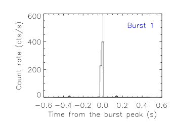
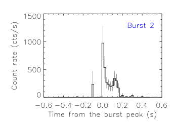
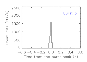
Figure 1.— Deadtime-corrected light curves of the bursts in the 3–79 keV band.

The spectrum of a burst can provide information on the burst mechanism. Therefore, we extracted $\sim$0.2-s spectra in circles with radius $R=120^{\prime\prime}$ centered at the source position for bursts 2 and 5, and fit the spectra with single component models; we tried both a blackbody and a power-law model. In order to remove the persistent emission, we extracted background counts in the same region as we used for the source but in a 1-ks pre-burst interval. We did not attempt to fit the burst data with a multi-component model because there were too few photons collected during the 0.2-s intervals. We grouped the spectrum to have 1 count per spectral bin, and used $lstat$ (Loredo, 1992) in XSPEC 12.8.1g. The NuSTAR bandpass is not sensitive to the relatively low $N_{\rm H}$ of the source, and we set it to $2.05\times 10^{22}\rm\ cm^{-2}$ which we obtained by joint-fitting of the soft-band spectra with a broken power-law model (see Section 3.2.3). We use this value and the tbabs absorption model in XSPEC throughout this paper unless noted otherwise. The burst spectra can be described with a power-law model having $\Gamma=1-2$ or a blackbody model with $kT=3-5\rm\ keV$. The results of the fits are shown in Table 3. Note that we did not detect the high temperature blackbody component ($kT=13$ keV Collazzi, Xiong, & Kouveliotou, 2014), which is probably because of the low statistics at high energy.

Table 3 Best-fit parameters of the burst spectra for a $\sim$0.2 s interval around the burst peak

Burst	$\Gamma$	3–79 flux	$lstat$/dof
		$10^{-8}\ \rm erg\ s^{-1}\ cm^{-2}$
2	1.6(3)	3.5(1.2)	37/46
5	0.96(24)	1300(600)	53/56
Burst	$kT$	$L_{\rm BB}^{\tablenotemark{b}}$	$lstat$/dof
	(keV)	$10^{38}\ \rm erg\ s^{-1}$
2	3.3(3)	1.5(3)	48/46
5	4.8(5)	400(100)	59/56

^a Deadtime-corrected flux.
^b Deadtime-corrected bolometric luminosity for an assumed distance of 8.5 kpc.

3.1.2 Burst Tails

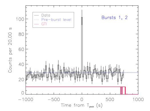
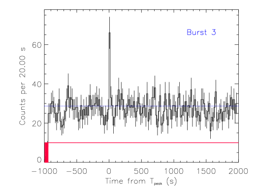
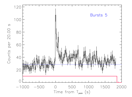
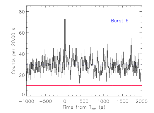
Figure 2.— Observed long-term light curves of the bursts in the 3–79 keV band. Note that bursts 1 and 2 are very close in time ($\stackrel{{\scriptstyle<}}{{{}_{\sim}}}$1 s), and that the light curve for burst 4 is not shown because the burst was not detected in a 20-s time bin. The blue dotted line shows the pre-burst emission level, and the red line shows the scaled Good Time Interval (GTI).

Short X-ray bursts from magnetars can exhibit long emission tails, lasting for hours (An et al., 2014). In order to search for long tails, we binned the light curves into 20-s bins, and compared counts in 10 bins before and after a burst, excluding the burst bin. We then compared the pre- and post-burst counts, and found that the difference is significant only for burst 5 ($\Delta_{\rm post-pre}=211\pm 43$ counts for a 200-s time interval). We show the light curves for the bursts in Figure 2, and report the results in Table 2. We performed the same study on different timescales (e.g., 2 s and 50 s), and found the same results; the difference is significant only for burst 5

In order to search for spectral evolution after burst 5, we extracted spectra within a radius $R=120^{\prime\prime}$ in the tail of burst 5 in several time intervals excluding the burst ($T>T_{\rm 0}+0.5$ s; see Table 2). Each interval had $\stackrel{{\scriptstyle>}}{{{}_{\sim}}}100$ events above the persistent emission plus background. We then fit the spectra with a blackbody and a power-law model. We show the results of the power-law fit in Figure 3. The spectral shape did not change significantly over $\sim$2-ks of tail emission, and the 3–79 keV flux decay is well described with a power-law function, having a decay index of $0.45\pm 0.10$. Note that the decay index was measured after taking into account the covariance between the flux and the spectral index in the fit. A similar decay index is measured for the luminosity when using a blackbody model. Note that An et al. (2014) measured the flux evolution index in the tail to be 0.8–0.9 for 1E 1048.1$-$5937, much steeper than our measurement for 1E 1841$-$045. The count enhancement at later times seems to be spiky, and might have been caused by undetected activity there. Since the other bursts do not have significant tail emission, we were not able to measure their spectral evolution.

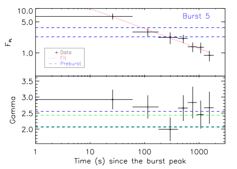
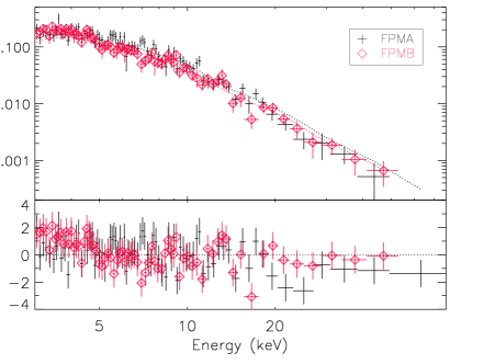
Figure 3.— Evolution of the persistent-emission-removed spectrum of the tail of burst 5 measured using a power-law model (left) and the integrated spectra (right). We used events collected after $T=T_{\rm 0}+0.5$ s to remove the burst emission. Flux is in units of $10^{-11}\rm\ erg\ s^{-1}\ cm^{-2}$ in the 3–79 keV band. The red dotted line in the left panel shows the power-law function that best describes the flux evolution, blue dashed lines show the 1$\sigma$ range of the quantities measured in a 100-s interval before the burst. The green dashed lines in the left bottom show the 1$\sigma$ range of the best-fit power-law index for the integrated tail spectrum. The integrated tail spectrum with a blackbody plus broken power-law fit with spectral shape parameters frozen at the values in Table 4 is shown in the right panel.

The tail spectrum of burst 5 is soft compared to the burst spectrum, and may be similar to the persistent emission. In order to see if the spectra of the burst tails are significantly different from the persistent source emission, we studied the persistent emission in a pre-burst interval in which approximately the same number of events was collected as in the tail spectra. We extracted a persistent spectrum in a 100-s pre-burst time interval, modeled it with a single component model, either a power law or a blackbody. The persistent spectrum over the short interval was well described with single component models, and we find the best-fit parameters are $\Gamma=2.31\pm 0.24$ or $kT=1.58\pm 0.13$ keV, similar to the tail spectrum. We show the persistent levels with blue dashed lines in Figure 4.

Since the spectral shape did not change significantly over the tail interval, we fit the combined ($\sim$1.8 ks) tail spectrum to a power-law or a blackbody model after removing the persistent emission. The spectrum is well fit by a power-law model ($\chi^{2}$/dof=122/146) with a photon index $\Gamma=2.2\pm 0.2$ (green lines in Figure 3 left), similar to the 100-s persistent spectrum. A blackbody model also fits the data with $kT=2.1\pm 0.2\rm\ keV$ ($\chi^{2}$/dof=137/146). We tried to fit the combined tail emission with the model for the persistent spectra obtained below (Section 3.2.3) using the same fit parameters except for the normalization constants (Table 4). The model fits the spectrum well ($\chi^{2}$/dof=171/147 with the null hypothesis probability $p=0.09$). However, we see a trend in the fit residuals which suggests that the tail spectra may be slightly softer than the persistent one (see Figure 3 right).

3.2. Persistent Emission

In order to study the persistent emission, we removed the burst intervals using time filters. We used 20-s windows centered at the burst peak times for all the bursts except for burst 5 for which we used a 2-ks window because of the tail. For the soft-band spectrum below 10 keV, we used the Chandra (only Obs. ID 730 due to pile-up in Obs. ID 6732), XMM-Newton, and Swift data (see Table 1), the same observations as used by A13. Although these observations were taken long before the NuSTAR observation, we show below that the source emission properties have been stable over 10 years (see also A13). For the NuSTAR data, we used a circular aperture with $R=60^{\prime\prime}$ for the source and an annular aperture with inner and outer radii of $R=60^{\prime\prime}$ and $R=100^{\prime\prime}$ for the background, respectively. Note that $\sim$15% of the source events fall in the background region because of the NuSTAR PSF (An et al., 2014). However, not all the $\sim$15% of the source flux is subtracted as background in the spectral fitting since we scale the area of the background region to that of the source for spectral fits, and $\sim$10% of source events will be lost during background subtraction. We take into account this effect using a normalization constant.

3.2.1 Timing Analysis

For our timing analysis, we extracted source events from the new observations in the 3–79 keV band within a radius $R=60^{\prime\prime}$ of the nominal source position, and divided the events into subintervals consisting of $\sim$5000 counts each. Note that we have used different subintervals and found that the results do not change significantly. Each subinterval was then folded at the nominal pulse period to yield pulse profiles each with 64 phase bins. In order to perform phase-coherent timing, we first cross-correlated the pulse profiles to measure the phase for each subinterval. We then fit the phases to a quadratic function using frequency ($\nu$) and its first derivative ($\dot{\nu}$), $\phi(t)=\phi_{0}+\nu(t-T_{\rm ref})+\dot{\nu}(t-T_{\rm ref})^{2}/2$, to derive a timing solution. We produced a high signal-to-noise ratio template by coherently combining the pulse profiles using the timing solution, and cross-correlated the pulse profiles with the template in order to refine the timing solution. We show the residuals after the fit in Figure 4. We find that the best timing solution during the observations has parameters $P=11.79234(1)\rm\ s$ and $\dot{P}=4.2(2)\times 10^{-11}\rm\ s\ s^{-1}$, implying a magnetic field strength of $7\times 10^{14}\rm\ G$. Note that we did not include the first NuSTAR observation (Obs. ID 30001025002) in this study because of phase ambiguity. We verified the timing solution by measuring the period for the individual observations including the first NuSTAR observation (Obs. ID 30001025002) using the $H$-test (de Jager et al., 1989), and by fitting the measured period to a linear function of period evolution $P(t)=P_{0}+\dot{P}(t-T_{\rm ref})\rm\ s$, which yields $P=11.792344(4)\rm\ s$ and $\dot{P}=4.05(9)\times 10^{-11}\rm\ s\ s^{-1}$. We find that the results of the two methods are consistent with each other and with the results of our Swift monitoring (see Section 4.1).

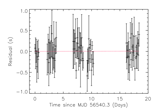
Figure 4.— Timing residuals after fitting the pulse phases in the 3–79 keV band for observations 30001025004–12.

3.2.2 Pulse Profiles and Pulsed Fraction

The pulse profile of 1E 1841$-$045 is known to change with energy (Kuiper et al., 2006; An et al., 2013). In particular, A13 found that the pulse shape in the 24–35 keV band is different from those in the adjacent energy ranges, which suggested the existence of a spectral feature. However, no firm conclusion could be made due to limited statistics. We investigate this here with much better statistics.

We produced pulse profiles for individual observations, and aligned them with the template. Backgrounds were extracted from an annular region with inner and outer radii of 60^′′ and 100^′′ and were subtracted from the pulse profile of the source region. We verified that the pulse shape has not changed significantly over the $\sim$300 days of NuSTAR observations (Table 1) by comparing the pulse profile of individual observations with the combined profile in several energy bands (e.g., 3–6 keV, 6–10 keV, 10–15 keV, and 15–79 keV). We show the combined pulse profiles in several energy bands in Figure 5. Note that we find double-peaked structure similar to that seen by A13, e.g., in the 17–33 keV band (see Figure 5). However, with the much better statistics we have now, we find that the pulse shape does not change suddenly but instead changes gradually with energy. This does not support the existence of a narrow spectral feature as suggested by A13.

We find that the pulse shape at higher energies becomes more complicated, sometimes showing three peaks (e.g., 33–38 keV in Figure 5; a new peak seems to appear at phase $\sim$0.5). In order to see if the triple-peaked structure at high energies ($\stackrel{{\scriptstyle>}}{{{}_{\sim}}}$ 25 keV) is significant, we fit each pulse profile with a harmonic function in which the number of harmonics contained was varied between zero (constant) and three. In the fit, we calculate the $\chi^{2}$ value and the F-test probability by adding higher-order harmonic functions one by one. From this study, we find that the pulse profiles below 38 keV are generally well fit with sum of two harmonics, and the others with a single harmonic function; adding one more harmonic to these is not statistically required (99% confidence). We further fit the pulse profiles with a sum of the first two harmonics plus a fifth harmonic because the triple-peaked structure is best described with a fifth harmonic. The F-test probability for adding the fifth harmonic shows an improvement to the fit with 99.7% confidence in the 45–55 keV band and with 98.6% confidence in the 33–38 keV band. However, these may not imply a significant detection when considering the number of double- peaked profiles we have. Therefore, we conclude that the double-peaked structures are statistically significant but the triple-peaked ones are only marginally so.

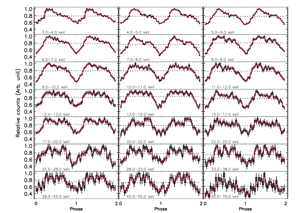
Figure 5.— Background-subtracted pulse profiles for 1E 1841$-$045 measured with NuSTAR in various energy bands. The average value is shown in a black dotted line and a Fourier reconstructed profile with five harmonics is shown in red in each panel.

The pulsed fraction of the source has previously been measured to be increasing with energy (Kuiper et al., 2006, A13). Note that A13 did not attempt to measure the area pulsed fraction defined by

$$PF_{\rm area}=\frac{\sum_{i}(p_{i}-p_{\rm min})}{\sum_{i}p_{i}},$$ (2)

where $p_{i}$ is counts in $i$-th phase bin and $p_{\rm min}$ is the counts from the lowest bin in the pulse profile, due to insufficient statistics, and that $PF_{\rm area}$ is known to be biased upwards in the low counts regime. Since we now have much better statistics, we measured the area pulsed fractions in different energy bands and show them in Figure 6. Even with good statistics, the area pulsed fraction is known to be biased upwards (see Appendix), and so we show two alternative measures of the pulsed fraction as well. The first alternative is to fit the pulse profile with a harmonic function, and use the best-fit function to calculate the pulsed fraction ($PF_{\rm fit}$), which will remove the bias caused by incorrect identification of the baseline level by selecting the minimum phase bin. We find that the pulse profiles are well described with two harmonics having $\chi^{2}$/dof$\sim$1 (Figure 5) except for the lowest energy band for which the two-harmonic function yields an unacceptable fit, with $p=10^{-4}$. The large $\chi^{2}$ in this case is mostly due to a sharp step in the pulse profile at phase $\sim$0.2, but the overall pulse shape agrees with the best-fit function well. Furthermore, rebinning the phase can make the fit acceptable. Therefore, we used two harmonics for the fit function, calculated $PF_{\rm area}$ using the best-fit parameters, and show the pulsed fractions in Figure 6 (blue squares). We also calculated the rms pulse amplitude defined by

$$PF_{\rm rms}=\frac{\sqrt{2\sum_{k=1}^{6}((a_{k}^{2}+b_{k}^{2})-(\sigma_{a_{k}}^{2}+\sigma_{b_{k}}^{2}))}}{a_{0}},$$ (3)

where

$$a_{k}=\frac{1}{N}\sum_{i=1}^{N}p_{i}\cos(\frac{2\pi ki}{N}),b_{k}=\frac{1}{N}\sum_{i=1}^{N}p_{i}\sin(\frac{2\pi ki}{N}),$$

$$\sigma_{a_{k}}^{2}+\sigma_{b_{k}}^{2}=\frac{1}{N^{2}}\sum_{i=1}^{N}\sigma_{p_{i}}^{2}\cos^{2}(\frac{2\pi ki}{N})+\frac{1}{N^{2}}\sum_{i=1}^{N}\sigma_{p_{i}}^{2}\sin^{2}(\frac{2\pi ki}{N})$$

is the Fourier power produced by the noise in the data, $p_{i}$ is the number of counts in $i$th bin, $N$ is the total number of bins, $\sigma_{p_{i}}$ is uncertainty in $p_{i}$, and $n$ is the number of Fourier harmonics included, in this case, $n=6$ (see Archibald et al., 2014, for more details). We show the results in Figure 6 (red diamonds).

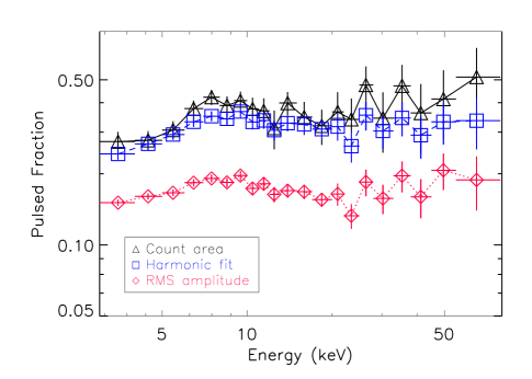
Figure 6.— Pulsed fractions at several energy bands measured with NuSTAR. Black triangles: area pulsed fraction (Equation 2); blue squares: area pulsed fraction measured using harmonic fit; and red diamonds: rms pulsed fraction (Equation 3).

We note that the small-scale features in Figure 6 change when we use different energy resolution. For example, a sudden jump sometimes appears at $\sim$30 keV similar to that seen by A13 (their Figure 3) if we use different energy bins. However, the overall trend is similar; we do not see any rapid increase in the pulsed fraction with energy above 10 keV. This is different from previous reports (Kuiper et al., 2006) of pulsed fraction increasing with energy and approaching 100% at 100 keV.

3.2.3 Phase-Averaged Spectral Analysis

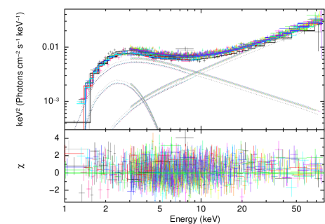
Figure 7.— Phase averaged spectra of 1E 1841$-$045 and the fit result. Chandra, XMM-Newton, and Swift data cover below 10 keV, and NuSTAR data cover 3–79 keV (see Table 1 for observation summary). Each component of the best-fit model, an absorbed blackbody plus double power law, is shown in lines. See Table 4 for best-fit model parameters.

Table 4Phenomenological spectral fit results for 1E 1841$-$045

Phase	Data	Energy	Model	$N_{\rm H}$	$kT$	$\Gamma_{\rm s}\tablenotemark{c}$	$E_{\rm break}/F_{\rm s}$	$\Gamma_{\rm h}$/$\beta$	$F_{\rm h}$	$L_{\rm BB}$	$\chi^{2}$/dof
		(keV)		($10^{22}\ \rm cm^{-2}$)	(keV)		(keV/ )
0.0–1.0	N,S,X,C	0.5–79	BB+BP	2.05(3)	0.491(5)	1.95(1)	13.5(2)/$\cdots$	1.24(1)	5.88(6)	1.64(5)	8060/7930
0.0–1.0	N,S,X,C	0.5–79	BB+2PL	2.49(5)	0.443(9)	2.82(8)	$\cdots$/1.53(6)	0.97(4)	4.70(6)	1.15(9)	7931/7930
Pulsed	N,X,C	0.5–79	PL	2.05	$\cdots$	$\cdots$	$\cdots$	1.83(3)	1.4(1)	$\cdots$	1236/1749
Pulsed	N	3–79	PL	2.05	$\cdots$	$\cdots$	$\cdots$	1.81(3)	1.4(1)	$\cdots$	1128/1591
Pulsed	N	5–79	PL	2.05	$\cdots$	$\cdots$	$\cdots$	1.73(4)	1.4(1)	$\cdots$	806/1140
Pulsed	N	10–79	PL	2.05	$\cdots$	$\cdots$	$\cdots$	1.47(7)	1.5(2)	$\cdots$	349/510
Pulsed	N	15–79	PL	2.05	$\cdots$	$\cdots$	$\cdots$	1.28(12)	1.6(3)	$\cdots$	174/279
Pulsed	N	20–79	PL	2.05	$\cdots$	$\cdots$	$\cdots$	1.0(2)	1.5(4)	$\cdots$	113/159

^a N: NuSTAR, S: Swift, X: XMM-Newton, C: Chandra.
^b BB: Blackbody, PL: Power law, BP: Broken power law, and 2PL: Two power laws in XSPEC.
^c Photon index for the soft power-law component.
^d Break energy for the BB+BP fit or soft power-law flux in units of $10^{-11}\ \rm erg\ s^{-1}\ cm^{-2}$ in the 3–79 keV for the BB+2PL fit.
^e Photon index for the hard power-law component.
^f Flux in units of $10^{-11}\rm\ erg\ cm^{-2}\ s^{-1}$. The values are only the power-law (hard power-law) flux in the 3–79 keV band for the BP (PL, 2PL) model.
^g Blackbody luminosity in units of $10^{35}\ \rm erg\ s^{-1}$ for an assumed distance of 8.5 kpc (Tian & Leahy, 2008).
^h $N_{\rm H}$ for the pulsed spectral analysis was frozen.

Since it is possible that the source has different emission properties during the bursting periods, we compared the spectral properties of individual observations. In this study, we did not include the soft-band spectra because they were taken at much earlier epochs. We jointly fit all the NuSTAR spectra in the 6–79 keV band with an absorbed broken power-law model in order to minimize the effect of the blackbody component, which is negligible above 6 keV, and found that the spectral shapes for the six NuSTAR observations (see Table 1) are consistent with one another.

Since there is no clear evidence that the source spectral shape has varied during the NuSTAR observations, we used all the NuSTAR observations for the phase-averaged spectral analysis. Furthermore, we used the soft-band data as well in this study since the shape of the soft-band spectrum is also known to be stable (Zhu & Kaspi, 2010; Dib & Kaspi, 2014). We tied all the model parameters between NuSTAR, Swift, XMM-Newton, and Chandra except for the cross-normalization factors. The normalization constant for NuSTAR FPMA (Obs. ID 30001025002) was set to be 0.9 as a reference in order to account for the source contamination in the background region (Section 3.2.2). To fit the data, we grouped the spectra to have at least 20 counts per bin. We used an absorbed blackbody plus broken power law, and an absorbed blackbody plus a double power law to fit the 3–79 keV NuSTAR data and the 0.5–10 keV soft-band data. We present the results in Table 4 and the spectra in Figure 7.

We note that the spectral parameters we report in Table 4 are slightly different from those reported previously (A13). In order to see if the difference is due to the updated calibration, we analyzed the same data set that A13 used (Obs. ID 30001025002), and were able to reproduce their results except for the flux. The flux we measure is lower by $\sim$15% than what A13 reported, because of a $\sim$15% increase in the NuSTAR effective area from CALDB 20131007. The hard-band component is much better constrained with the new long exposures, and thus the new results we report are more accurate. We note that the new parameters in Table 4 are not inconsistent with the data A13 used, providing acceptable fits to the data with $\chi^{2}$/dof =2965/2878 and 2914/2878 for the blackbody plus broken power law and the blackbody plus double power law, respectively.

3.3. Phase-Resolved and Pulsed Spectral Analyses

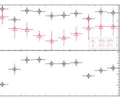
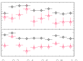
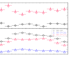
Figure 8.— Results of our phase-resolved spectral analysis. Blackbody luminosity ($L_{\rm BB}$) is in units of $10^{35}\ \rm erg\ s^{-1}$, and power-law flux ($F_{\rm PL}$) is in units of $10^{-11}\ \rm erg\ s^{-1}\ cm^{-2}$ in the 3–79 keV band. Gamma_h is the power-law index of the hard power-law component and Gamma_s is for the soft component.

We conducted a phase-resolved spectral analysis for ten phase intervals to study distinct features in the pulse profiles (see Figure 5 for pulse profiles). We did not use the Swift XRT or XMM-Newton MOS data in this study because their temporal resolutions were insufficient. The Chandra and XMM-Newton PN data were phase-aligned with the NuSTAR data by correlating the pulse profiles.

We binned the NuSTAR and soft-band instrument spectra to have at least 20 counts per spectral bin, and froze the cross-normalization factors to those obtained with the phase-averaged spectral fit. We fit the spectra with the two models that we used for fitting the phase-averaged spectrum: an absorbed blackbody plus broken power law and an absorbed blackbody plus double power-law model. We find that both models explain the data well, having $\chi^{2}$/dof$\stackrel{{\scriptstyle<}}{{{}_{\sim}}}$1.003 for dofs of 1413–1966. The spectra vary with spin phase, having harder power-law spectra when the flux is high. However, the detailed variation depends on the spectral model used. We show the results in Figure 8.

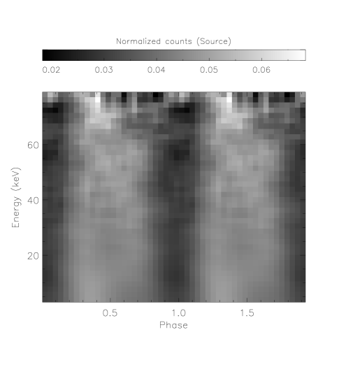
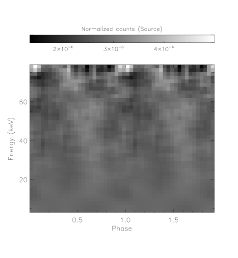
Figure 9.— Background-subtracted energy-phase count images in the 3–79 keV band produced using 25 phase bins and 40 energy bins. Counts in each pixel were divided by the phase-integrated counts in the same energy bin (left), and then by the energy-integrated counts in the same phase bin (right). Two phases are displayed for clarity.

In order to see if there is a spectral feature that shifts with energy as was seen in SGR 0418+5729 (Tiengo et al., 2013), we produced an energy-phase image using 25 phase bins and 40 energy bins in the 3–79 keV band. We first divided counts in each pixel in the energy-phase 2-D map by the phase-integrated counts in the same energy bin and present it in the left panel of Figure 9, which shows similar structures to the energy-resolved pulse profiles (Figure 5). We then divided the map further by the energy-integrated counts in the same phase bin (Figure 5) in order to have a better contrast, and find no clear phase-dependent feature in the image (Figure 5 right). We also tried different binning and found the same results.

We measured the pulsed spectrum in the 0.5–79 keV band in order to see if it is significantly harder than the phase-averaged spectrum as seen in other hard X-ray bright magnetars (Kuiper et al., 2006). We grouped the spectra to have at least 200 counts per spectral bin and subtracted the spectrum in the phase interval 0.9–1.1 (the DC level) from the phase-averaged spectra obtained in Section 3.2.3. We then jointly fit the broad-band spectrum with a power-law model letting the cross normalization constants vary. We used lstat and $\chi^{2}$ statistics and found that they give consistent results.

A simple power-law model with a photon index of 1.8 fits the 0.5–79 keV data well (reduced $\chi^{2}$/dof$<$1). In order to verify the measurements for the pulsed spectrum above 15 keV ($\Gamma=0.72\pm 0.15$, Kuiper et al., 2006), we restricted the fit range to high energies. As the lower energy cutoff is increased, the power-law index decreases, consistent with spectral hardening. The results are summarized in Table 4.

We also estimated pulsed fractions in the hard band using the spectra (defined as the ratio of pulsed and total flux densities) in order to compare with those in Figure 6. We fit the total and the pulsed spectra ($\stackrel{{\scriptstyle>}}{{{}_{\sim}}}$15 keV) to single power-law models. The power-law index of the total spectrum above 15 keV is $1.19\pm 0.02$ ($1.13\pm 0.02$ above 20 keV), slightly smaller than what we obtained using the absorbed blackbody plus broken power-law model (see Table 4). The power-law index of the pulsed spectrum above 15 keV is $1.28\pm 0.12$ ($1.0\pm 0.2$ above 20 keV), similar to that of the total spectrum. This suggests that the pulsed flux does not rapidly increase in the hard band, as also seen in Figure 6.

3.4. Spectral fits with the $e^{\pm}$ outflow model

A13 found that the properties of the persistent hard X-ray emission of 1E 1841$-$045 was consistent with the coronal outflow model proposed by Beloborodov (2013). The model envisions an outflow of relativistic electron-positron pairs created by electric discharge near the neutron star. The outflow fills the active “$j$-bundle” — a bundle of closed magnetospheric field lines that carry electric current (Beloborodov, 2009). The pair plasma flows out along the magnetic field lines and gradually decelerates as it scatters the thermal X-rays. It radiates most of its kinetic energy in hard X-rays before the $e^{\pm}$ pairs reach the top of the magnetic loop and annihilate. The magnetic dipole moment of 1E 1841$-$045 is estimated from its spin-down rate, $\mu\approx 7\times 10^{32}\rm\ G\ cm^{3}$, assuming the neutron star radius to be 10 km. Similar to A13 and Hascoët, Beloborodov & den Hartog (2014), we assume a simple geometry where the $j$-bundle is axisymmetric around the magnetic dipole axis. However, instead of assuming that the $j$-bundle emerges from a polar cap, its footprint is allowed to have a ring shape. This possibility was introduced in Vogel et al. (2014), because the NuSTAR data for 1E 2259$+$586 favored a ring footprint over a polar cap. The model has the following parameters: (1) the power $L_{j}$ of the $e^{\pm}$ outflow along the $j$-bundle, (2) the angle $\alpha_{\rm mag}$ between the rotation axis and the magnetic axis, (3) the angle $\beta_{\rm obs}$ between the rotation axis and the observer’s line of sight, (4) the angular position $\theta_{j}$ of the $j$-bundle footprint, and (5) the angular width $\Delta\theta_{j}$ of the $j$-bundle footprint. In addition, the reference point of the rotational phase, $\phi_{\rm 0}$, is a free parameter, since we fit the phase-resolved spectra.

We follow the method presented in Hascoët, Beloborodov & den Hartog (2014) and explore the whole parameter space by fitting the phase-averaged spectrum of the total emission (pulsed+unpulsed) and phase-resolved spectra of the pulsed emission. We use five equally spaced phase intervals. NuSTAR data are fitted above 10 keV, where the coronal outflow has to account for most of the observed emission.

$p$-value

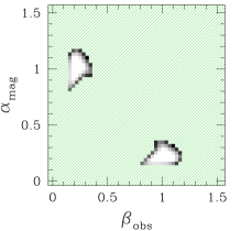
Figure 10.— Map of $p$-values for the fit of the hard X-ray component with the coronal outflow model; the $p$-values are shown in the plane of ($\alpha_{\rm mag}$, $\beta_{\rm obs}$) and maximized over the other parameters. The $p$-value scale is shown on the left. The hatched green region has $p$-values smaller than $0.001$; the white region has $p$-values greater than $0.1$. Interchanging the values of $\alpha_{\rm mag}$ and $\beta_{\rm obs}$ does not change the model spectrum, as long as the $j$-bundle is assumed to be axisymmetric. Therefore, the map of $p$-values is symmetric about the line of $\beta_{\rm obs}=\alpha_{\rm mag}$.

Figure 10 shows the map of the $p$-value of the fit in the $\alpha_{\rm mag}$-$\beta_{\rm obs}$ plane. The acceptable model is clearly identified in this map. It has $\alpha_{\rm mag}=0.25\pm 0.15,\beta_{\rm obs}=1.0\pm 0.2$, $\theta_{j}=0.24\pm 0.02$, and $\Delta\theta_{j}/\theta_{j}>0.26$, consistent with a polar cap. The corresponding magnetic flux in the $j$-bundle is $(2.5\pm 0.4)\times 10^{26}\rm\ G\ cm^{2}$. The power dissipated in the $j$-bundle is $L_{j}=(6\pm 1)\times 10^{36}\rm\ erg\ s^{-1}$. Most of the released energy is radiated in the MeV band (peaking at $\sim$6 MeV) and is not seen to NuSTAR. Using the obtained best-fit model for the hard X-ray component, we have investigated the remaining soft X-ray component. The procedure is similar to that in A13 and Hascoët, Beloborodov & den Hartog (2014); we freeze the best-fit parameters of the outflow model and fit the spectrum in the 0.5–79 keV band using the NuSTAR, Swift, Chandra, and XMM-Newton data. As in A13, we find that the 0.5–79 keV spectrum is well fitted by the sum of two blackbodies (which dominate below 10 keV) and the coronal outflow emission (which dominates above 10 keV). The cold and hot blackbodies have luminosities $L_{c}=2.2\pm 0.1\times 10^{35}\rm\ erg\ s^{-1}$, $L_{h}=9.8\pm 1.3\times 10^{34}\rm\ erg\ s^{-1}$ and temperatures $kT_{c}=0.45\pm 0.01\rm\ keV$, $kT_{h}=0.75\pm 0.02\rm\ keV$. Note that these values are different from those we obtained with the phenomenological models in Table 4.

4. Swift monitoring observations

We report below on Swift monitoring observations for spectral and temporal behavior of the source on long timescales. The observations were taken with the X-Ray Telescope (XRT) using Windowed-Timing (WT) mode for all observations, which have been conducted once every two to three weeks since 2011 July, except when the source was in Sun-constraint from mid-November to mid-February each year. In total, 68 observations (not listed in Table 1) having $\sim$266 ks of summed exposure were analyzed. The Swift data were processed with xrtpipeline using the HEASARC remote CALDB.

4.1. Data Analysis and Results for the Swift Monitoring Observations

To investigate the spectrum of 1E 1841$-$045 in the monitoring observations, we extract spectra for each observation using a 10-pixel (24^′′) long strip centered on the source. An annulus of inner radius 75-pixel, and outer radius 125-pixel centered on the source was used to extract background spectra. The spectra were grouped to have a minimum of 20 counts per bin. The spectra were fitted with a photoelectrically absorbed blackbody with an added power-law component, using the tbabs(bbody+pow) model in XSPEC 12.8.1, with $N_{\rm H}$ held fixed at $2.05\times 10^{22}\rm\ cm^{−2}$, the value we obtained in Section 3.2.3. No significant change in source 1–10 keV flux was observed over the monitoring period of $\sim$3 years ($\chi^{2}$/dof=49/59), including the NuSTAR-observed bursting period. The result is shown in Figure 11 (a).

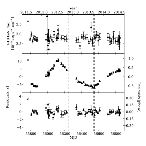
Figure 11.— Results of the Swift monitoring campaign for flux and timing. (a) 1–10 keV flux, (b) timing residuals after fitting out $\nu$ and $\dot{\nu}$, and (c) after fitting out twelve frequency derivatives. Vertical dashed lines show the periods when NuSTAR observations were taken.

We also searched all the Swift observations for bursts by binning the source region light curves above 1 keV into 0.01 s, 0.1 s, and 1.0 s bins. The counts in each bin were compared to the mean count rate of its GTI, assuming the Poisson distribution. We found no significant bursts in the Swift XRT data. Note that the Swift observations did not cover the NuSTAR-detected bursts times presented in Table 2.

In order to derive the timing solution and to search for glitching activity, we barycentered the source events using the location of 1E 1841$-$045, R.A.=$18^{h}41^{m}19.34^{s}$, Decl.=$-4^{\circ}56^{\prime}11\farcs 2$. We then extracted Time-Of-Arrivals (TOA) using a Maximum Likelihood (ML) method (see Livingstone et al., 2009; Scholz et al., 2012). The ML method compares a continuous model of the pulse profile to the profile obtained by folding a single observation. These TOAs were fitted to a pulse arrival model (e.g., the quadratic function in Section 3.2.1) using the TEMPO2 (Hobbs, Edwards & Manchester, 2006) pulsar timing software package. We find that a timing model consisting of $\nu$ and $\dot{\nu}$ does not fit the data well (Figure 11 (b) and “Fit 1” in Table 5) as was already observed in the previous RXTE monitoring observations (e.g., see Dib & Kaspi, 2014). We need to include twelve frequency derivatives in order to achieve an acceptable fit (i.e., $\chi^{2}$/dof$\sim$1) with Gaussian residuals (Figure 11 (c) and “Fit 2” in Table 5). Note that the timing solutions presented in Table 5 are valid only over the time interval of the monitoring campaign.

Motivated by the apparent ‘kink’ in the residuals of the simple spin-down model around MJD 56100, we attempted to fit a glitch at the epoch of the kink. However, the data are better fit using a model with four frequency derivatives (rms residual of 0.97 s) versus a glitch model (rms residual of 0.99 s). Therefore we do not need to invoke a sudden event to explain the measured TOAs. We present our best timing solutions in Table 5.

Table 5Timing Parameters for 1E 1841$-$045.

RA (J2000)	$18^{h}41^{m}19.34^{s}$
DEC (J2000)	$-4^{\circ}56^{\prime}11.2^{\prime\prime}$
MJD Range	55795-56799
Epoch (MJD)	56300
Fit 1
$\nu$ (s-1)	0.084 806 860 6(9)
$\frac{d^{1}\nu}{dt^{1}}$ (s-2)	$-$2.9121(8)$\times 10^{-13}$
RMS (s)	4.82
$\chi^{2}$/dof	2889.05/53
Fit 2
$\nu$ (s-1)	0.084 806 897(4))
$\frac{d^{1}\nu}{dt^{1}}$ (s-2)	$-$2.985(12)$\times 10^{-13}$
$\frac{d^{2}\nu}{dt^{2}}$ (s-3)	6.8(23)$\times 10^{-22}$
$\frac{d^{3}\nu}{dt^{3}}$ (s-4)	4.6(8)$\times 10^{-28}$
$\frac{d^{4}\nu}{dt^{4}}$ (s-5)	$-$8.7(16)$\times 10^{-35}$
$\frac{d^{5}\nu}{dt^{5}}$ (s-6)	$-$2.5(5)$\times 10^{-41}$
$\frac{d^{6}\nu}{dt^{6}}$ (s-7)	6.0(12)$\times 10^{-48}$
$\frac{d^{7}\nu}{dt^{7}}$ (s-8)	1.2(3)$\times 10^{-54}$
$\frac{d^{8}\nu}{dt^{8}}$ (s-9)	$-$3.4(7)$\times 10^{-61}$
$\frac{d^{9}\nu}{dt^{9}}$ (s-10)	$-$4.5(10)$\times 10^{-68}$
$\frac{d^{10}\nu}{dt^{10}}$ (s-11)	1.4(3)$\times 10^{-74}$
$\frac{d^{11}\nu}{dt^{11}}$ (s-12)	9.5(22)$\times 10^{-82}$
$\frac{d^{12}\nu}{dt^{12}}$ (s-13)	$-$3.3(8)$\times 10^{-88}$
RMS (s)	0.43
$\chi^{2}$/dof	49.34/42

Notes. All errors are TEMPO2 reported 1$\sigma$ errors.

5. Discussion

The new 350-ks observation of 1E 1841−045 by NuSTAR allowed a significantly better study of its persistent emission and the serendipitous detection of X-ray bursts. Below we discuss the results and compare them with observations of other magnetars.

5.1. The X-ray Bursts and the Tails

Magnetars often show bursting behavior in the X-ray band, which may be caused by instabilities inside the neutron star or its magnetosphere (Thompson & Duncan, 1995; Lyutikov, 2003; Woods & Thompson, 2006). The time profiles and spectra of bursts show significant diversity. Woods et al. (2005) suggested that there are two types of magnetar bursts, one having significant tail emission and the other having orders of magnitude smaller tail emission. The authors attributed the former to crustal activity and the latter to magnetospheric activity. Lenters et al. (2003) found a strong correlation between bursts and tail energies in the magnetar SGR 1900$+$14.

The X-ray bursts from 1E 1841$-$045 in 2013 September have very short rise and fall times, with $T_{\rm 90}$ of 0.01–0.6 s, and hard spectra ($\Gamma$=1–2 or $kT\sim$3–5 keV). The blackbody temperature we measured for the burst 5 ($4.8\pm 0.5$ keV; see Table 3) is consistent with that of the colder blackbody measured with the GBM ($kT_{l}=5.3\pm 0.2$ keV; Collazzi, Xiong, & Kouveliotou, 2014).

Kumar & Safi-Harb (2010) reported detection of emission lines at 27 keV, 40 keV and 60 keV in the 2010 May burst spectrum with Swift BAT, although these are argued against later by Lin et al. (2011). Interestingly, all the lines are in the NuSTAR band, and could be detected by NuSTAR if they appeared again. However, we do not see evidence of line emission. Therefore, we estimate 90% upper limits on any 27 keV Gaussian line flux to be 0.24 photons $\rm cm^{-2}\ s^{-1}$ and 0.11 photons $\rm cm^{-2}\ s^{-1}$ in the brightest burst spectrum for the blackbody and the power-law continuum models, respectively. Note that we are not able to compare our results with those of Kumar & Safi-Harb (2010) since they did not present the line flux.

An extended tail is reliably detected only in energetic burst 5, and we find a hint of a tail in burst 6. Note that these two bursts were also observed by the GBM, and had significant flux above the NuSTAR band (Collazzi, Xiong, & Kouveliotou, 2014); they are the two most energetic bursts in our sample. Thus, the tail brightness and the burst energy we measure for the 1E 1841$-$045 bursts seem to agree qualitatively with the correlation reported for SGR 1900$+$14 and SGR 1806$-$20 (Lenters et al., 2003; Göğüş et al., 2011). A similar trend was also seen in the recent bursts from 1E 1048.1$-$5937 (An et al., 2014). We note however that the large energy seen by GBM in bursts 5 and 6 indicates a tail-to-burst ratio ($E_{\rm tail}/E_{\rm burst}\sim 2\times 10^{-2}$) that is much lower than in 1E 1048.1$-$5937 ($E_{\rm tail}/E_{\rm burst}\sim 5$–$60$). This confirms the known diversity of tails of magnetar bursts (Kaspi et al., 2004; Woods et al., 2005). Whether the tail-to-burst ratio follows a bimodal or a random distribution is not yet clear, and further investigation is required.

In contrast to the burst tails observed by NuSTAR for 1E 1048.1$-$5937, the burst tail in 1E 1841$-$045 shows no clear correlation between spectral hardness and flux. This correlation was also absent in some of the long-term (months to years) flux relaxation of other magnetars (e.g., An et al., 2012).

The flux evolution in the tail of burst 5 followed a power-law decay with a decay index of $0.45\pm 0.10$. The flux decay is similar to the tails of bursts from SGR 1900$+$14 (decay index of 0.43–0.7; Lenters et al., 2003). A significantly faster decay was observed for burst tails in 1E 1048.1$-$5937 (decay index of 0.8–1; An et al., 2014). It is possible that the tail contains many unresolved weaker bursts which affect the observed flux decay. It is still unclear what controls the resulting decay rate and why it is significantly different in 1E 1048.1$-$5937 and 1E 1841$-$045.

Furthermore, we find that the tail spectra in 1E 1841$-$045 are similar to (or slightly softer than) the persistent emission. In contrast, the tail spectra in 1E 1048.1$-$5937 were significantly harder than its persistent emission. This further contributes to the diversity of magnetar bursts. For instance, 1E 2259$+$586 exhibited bursts with and without ks-long tails, and the tail emission was observed to soften with decreasing flux (Kaspi et al., 2004). The observed diversity of magnetar bursts is not well explained by current theoretical models.

5.2. Pulse Profile and Pulsed Fraction

It is known that the pulse profiles of magnetars can look significantly different in different energy bands (den Hartog et al., 2008). This is also true for 1E 1841$-$045 (Figure 5). An interesting feature of the pulse profile is the double-peaked structure in the narrow band of $\sim$24–35 keV. A13 found this in the previous NuSTAR observation, and suggested that it may be caused by a spectral feature. The new long observation confirms the double peaked structure. It shows however that the change in the pulse profile is not as sharp as was suggested previously, and its shape may be more complicated, as a hint of another peak appearing between the two peaks is seen in several energy bands (e.g., in the 33–35 keV profile in Figure 5).

The pulsed fraction (and the rms pulse amplitude) increases with photon energy below $\sim$8 keV (Figure 5). We found no significant increase in the pulsed fraction above 8 keV, in contrast with previous measurements (Kuiper et al., 2006). This conclusion is insensitive to the choice of energy bins in Figure 5, which can affect the measured values in individual bins, but not the general trend. Our spectral analysis also suggests that the pulsed and steady components of the flux have similar power-law photon indices at high energies $>$15 keV (see Section 3.3 and Table 4). In the coronal outflow model, this implies that one of the angles, $\alpha_{\rm mag}$ and $\beta_{\rm obs}$, is small, or the emission region ($\theta_{j}$) is broad.

5.3. Spectra

We have measured the phase-averaged, phase-resolved and pulsed spectra of the source. Our best-fit parameters are slightly different from those reported by A13. The use of the new CALDB for the NuSTAR data may have some effect on the obtained spectral shape, however we showed in Section 3.2.3 that this effect is small.

We do not see any significant change in the source flux among the observations taken over one year despite the fact that bursts were detected in some observations but not in the others. We further compared the NuSTAR-measured spectrum with that reported previously ($\Gamma=1.32\pm 0.11$ and $L_{\rm 10-100keV}=3.0\times 10^{35}\rm\ erg\ s^{-1}$ for an assumed distance of 6.7 kpc; Kuiper et al., 2006), and find that our measurement ($\Gamma=1.37\pm 0.01$ and $L_{\rm 10-100keV}=3.0\times 10^{35}\rm\ erg\ s^{-1}$) is fully consistent with the previous values, suggesting that the source hard-band spectrum has been stable over 10 years. The same trend in the soft band (1–10 keV) is seen in the Swift monitoring data (see Figure 11). Stability in the soft-band pulsed flux has been reported by Dib & Kaspi (2014) and Zhu & Kaspi (2010) for a longer period. We note that Kumar & Safi-Harb (2010) reported a possible increase in the soft-band flux for 1E 1841$-$045 ($<$10 keV) associated with the source burst activity. However, Lin et al. (2011) showed that there is no significant change in the soft-band flux over a 1400-day interval, including the burst period reported by Kumar & Safi-Harb (2010).

The new measurements of the phase-resolved spectrum agree with the previous NuSTAR observation. The spectrum is harder near the pulse peaks, with smaller $\Gamma_{\rm h}$ and greater $E_{\rm break}$. We also note a possible hardening of the phase-averaged spectrum above $>$15 keV. However, we cannot reliably measure the spectrum curvature in the hard X-ray band due to the statistical noise.

We have searched for the spectral feature that was suggested as a possible explanation for the change in the pulse profile near 30 keV (A13). We find that the phase-resolved spectra are all well fit by a blackbody plus broken power law or a blackbody plus double power law; no emission or absorption line is required or hinted at by the fit residuals. We also searched for a spectral feature that shifts with rotational phase as was seen in SGR 0418$+$5729 (Tiengo et al., 2013), but did not find such a feature (Figure 9).

5.4. Outflow model

The more accurate phase-resolved spectrum obtained from the 350-ks NuSTAR observation provides a new opportunity to apply the coronal outflow model. We found that the model still fits the observed hard X-ray spectrum, and it does so in a small region of the parameter space (Figure 10), which allowed us to estimate the size of the active $j$-bundle, the dissipated power in the magnetosphere, and the angles between the magnetic axis, the rotation axis, and the line of sight. The increase in exposure by a factor $\sim$6 excluded at more than 3$\sigma$ level the second solution for the outflow model that was found in A13.

Interestingly, adding the new free parameter $\Delta\theta_{j}$ does not introduce new acceptable solutions (with a $p$-value above $10^{-3}$) and does not significantly affect the best solution — the best fit shows that the footprint of the $j$-bundle on the star is a broad ring, hardly distinguishable from a polar cap. This contrasts with 1E 2259$+$586, where a thin ring with $\Delta\theta_{j}/\theta_{j}<0.2$ is clearly statistically favored over a polar cap. This diversity may point to different distributions of the crustal magnetic stresses which are responsible for the magnetospheric twisting.

The soft X-ray component (below $\sim$10 keV) is well fitted by the sum of two blackbodies. The best-fit model is similar to that found in A13. The cold blackbody covers a large fraction of the star area, $\mathcal{A}_{c}\approx 0.42\mathcal{A}_{\rm NS}$, where $\mathcal{A}_{\rm NS}$ is the area of the neutron star with an assumed radius $R_{\rm NS}=10\rm\ km$. The emission area of the hot blackbody, $\mathcal{A}_{h}\approx 0.024\mathcal{A}_{\rm NS}$, is comparable with the area of the outflow footprint $\mathcal{A}_{j}=\pi\sin^{2}\theta_{j}\simeq 0.014\ (\theta_{j}/0.24)^{2}$. This is consistent with the coronal outflow model, where the footprint of the $j$-bundle is expected to form a hot spot, as some particles accelerated in the $j$-bundle flow back to the neutron star and bombard its surface.

Figure 10 suggests that the coronal outflow correctly describes the hard X-ray source as a decelerating $e^{\pm}$ outflow ejected from a discharge zone near the star. The outflow parameters inferred from the fit of the phase-resolved data have rather small statistical uncertainties, and the results reveal a puzzling feature of 1E 1841$-$045. Using Equation (48) in Beloborodov (2009), one can infer the discharge voltage in the active $j$-bundle: $\Phi\approx 10^{11}\psi^{-1}\ \mathrm{V}$ where $\Psi$ is the twist implanted in the magnetosphere, which does not exceed $\psi_{\rm max}\sim 3$ (Parfrey, Beloborodov & Hui, 2013). Due to our refined constraint on $\theta_{j}$ and the strong dependence of $\Phi$ on $\theta_{j}$ ($\Phi\propto\theta_{j}^{4}$), the inferred voltage is one order of magnitude higher than that given in A13. The high voltage is surprising in two ways: (1) it exceeds the expected threshold for $e^{\pm}$ discharge (Beloborodov & Thompson, 2007) by at least a factor of 10; (2) it implies a short timescale for ohmic dissipation of the magnetospheric twist $t_{\rm diss}\approx 0.1\,\psi^{2}$ yr (Equation (50) in Beloborodov, 2009). Thus, without continued energy supply, the $j$-bundle is expected to untwist on a year timescale or faster, which is not observed — the persistent X-ray emission from 1E 1841$-$045 has been stable for at least one decade.

This puzzle is related to a more general question: why are some magnetars transient and others persistent? The magnetospheric activity should be fed by magnetic energy pumped from the star by its surface motions. The surface motions are caused by the crust yielding to accumulating magnetic stresses inside the magnetar. Energy supply to the twisted magnetosphere may or may not be intermittent, depending on the mechanism of the crustal motions. Beloborodov & Levin (2014) have recently shown that the crust can yield through a thermoplastic instability which launches a slow wave resembling the deflagration front in combustion physics. The thermoplastic wave rotates the crust and twists the magnetosphere. This mechanism naturally triggers the outbursts observed in transient magnetars, yet it is still unclear how the quasi-steady state observed in 1E 1841$-$045 is formed. It could be formed by frequently repeated energy supply to the $j$-bundle combined with some form of feedback on its untwisting rate.

5.5. Swift monitoring observations

We did not detect any changes in the 1–10 keV source flux during the three years of Swift-XRT monitoring since 2011. In particular, the flux did not change significantly during the bursting period, which is consistent with the stability of persistent emission in the NuSTAR data. Our measurements do not agree with the observation that the source persistent emission properties changed due to bursts (Kumar & Safi-Harb, 2010). Note that Lin et al. (2011) also observed no change in the persistent properties of the source after bursts. The flux stability also implies that the source seems to be in a perpetually bursting state, and perhaps this is a difference between the classical bright AXPs monitored with RXTE and ‘transient’ sources, i.e., perhaps the bursting indicates that there is more heat dissipating and hence more magnetic activity in this magnetar, consistent with the higher $L_{\rm X}$ in “quiescence”.

The pulse timing behavior of 1E 1841$-$045 is known to be noisy, and Dib & Kaspi (2014) had to use five derivative terms to fit the timing data. Our timing solution requires twelve frequency derivatives. Note that although Dib & Kaspi (2014) used a much longer data span (13 yr), they break the data into smaller pieces which span 1–3 yr, similar to ours. The Swift monitoring data require more frequency derivatives than the RXTE data do due to the large kink at MJD 56100 which may indicate a glitch. We investigated the possibility that the kink is caused by a glitching activity but did not find any evidence of a glitch during the monitoring period of 3 years including the bursting period.

6. Conclusions

During NuSTAR observations of the magnetar 1E 1841$-$045, we detected six X-ray bursts from the source. The bursts are short, $T_{\rm 90}<1$ s, and bright. A tail was observed after one burst which was most energetic as measured with Fermi GBM. The tail emission was similar to or softer than the persistent emission, and the flux decay in the tail followed a power law with a decay index of $\sim$0.5, with no clear spectral softening with time. The properties of the tail emission are different from those seen after recent NuSTAR-observed X-ray bursts from the magnetar 1E 1048.1$-$5937 whose tails decayed fast with flux decay indices of 0.8–0.9 and had harder spectra than the persistent emission. The new observations also yield detailed pulse profiles in different energy bands, and show that the pulsed fraction does not increase rapidly with energy, in contrast to previous observational reports. We show that the source hard-band flux has been stable over $\sim$10 years. Using a Swift monitoring campaign, we found that the 1–10 keV flux from the source has been stable within $<$20% and the source timing behavior has been very noisy during a 3-year period, in spite of the bursting behavior we have observed.

The X-ray spectra of 1E 1841$-$045 are well fitted by the coronal outflow model of Beloborodov (2013). The new fit has provided improved constraints on the angle between the magnetic and rotation axes of the magnetar and the size of its active $j$-bundle. Remarkably, the best fit implies fast dissipation of the magnetic twist, in apparent contradiction with the observed stability of X-ray emission, as no long-term evolution has been detected in the persistent emission of 1E 1841$-$045 for more than one decade (Kuiper et al., 2006, A13). This behavior is distinct from the untwisting magnetospheres in transient magnetars and presents a puzzle that is yet to be resolved.

This work was supported under NASA Contract No. NNG08FD60C, and made use of data from the NuSTAR mission, a project led by the California Institute of Technology, managed by the Jet Propulsion Laboratory, and funded by the National Aeronautics and Space Administration. We thank the NuSTAR Operations, Software and Calibration teams for support with the execution and analysis of these observations. This research has made use of the NuSTAR Data Analysis Software (NuSTARDAS) jointly developed by the ASI Science Data Center (ASDC, Italy) and the California Institute of Technology (USA). H.A. acknowledges supports provided by the NASA sponsored Fermi Contract NAS5-00147 and by Kavli Institute for Particle Astrophysics and Cosmology. V.M.K. acknowledges support from an NSERC Discovery Grant and Accelerator Supplement, the FQRNT Centre de Recherche Astrophysique du Québec, an R. Howard Webster Foundation Fellowship from the Canadian Institute for Advanced Research (CIFAR), the Canada Research Chairs Program and the Lorne Trottier Chair in Astrophysics and Cosmology. A.M.B. acknowledges the support by NASA grant NNX13AI34G.

Appendix A COMPARISON BETWEEN ESTIMATORS OF PULSED FRACTION

Some confusions on pulsed fraction of a pulsar have been arisen mainly because different literatures use a different estimator. In this appendix, we review several commonly used estimators of pulsed fraction, and describe cautions to be taken when using them.

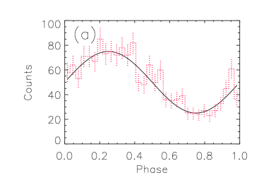
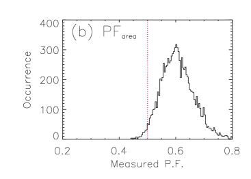
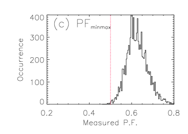
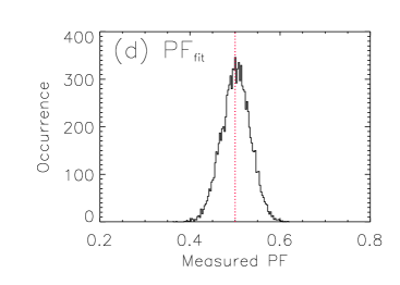
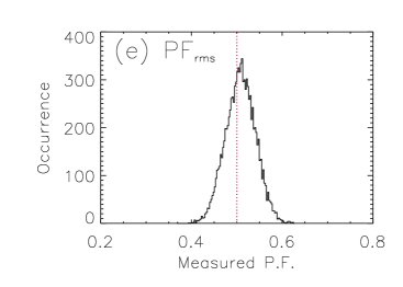
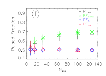
Figure 12.— Simulation results: (a) pulse profiles where the solid line is a theoretical pulse profile, and the dotted curve shows a realization of the theoretical pulse profile, and pulsed fractions measured using (b) area fraction ($PF_{\rm area}$), (c) min-max bin ($PF_{\rm minmax}$), (d) a function fit ($PF_{\rm fit}$), (e) rms amplitude ($\sqrt{2}PF_{\rm rms}$), and (f) for different binning. Vertical red dotted line in panels (b)-(f) shows the theoretical value for the pulsed fraction.

We consider four different estimators of pulsed fraction commonly used in literatures: pulsed fraction measured by (1) count area $PF_{\rm area}$ (Equation 2), (2) min-max counts, $PF_{\rm minmax}=\frac{p_{\rm max}-p_{\rm min}}{p_{\rm max}+p_{\rm min}}$, (3) fitting the light curve ($PF_{\rm fit}$), and (4) calculating rms variation ($\sqrt{\frac{\sum_{i}(p_{i}-<p>)^{2}}{<p>^{2}}}$) using truncated Fourier series and subtracting Fourier power produced by noise in the pulse profile, $\sigma_{a_{k}}^{2}+\sigma_{b_{k}}^{2}$, from the Fourier amplitudes ($PF_{\rm rms}$, Equation 3, see also Archibald et al., 2014). As we show below, estimators (1) and (2) are biased upwards since one has to select the minimum (and maximum) count bin in the pulse profile. For example, if the DC component of a pulse profile is relatively broad, one of the DC bins will very likely fall below the “true” minimum because of statistical fluctuation. Since one will use that phase bin for $p_{\rm min}$, the resulting pulsed fraction will be higher than the true value. Although this bias can be avoided by holding the minimum phase ($\phi_{\rm min}$) fixed and performing simulations, the spread in the measurements will be larger in this case than in the case of picking up the minimum bin as we show below.

Table 6Summary of measurements made with 10,000 simulations

Estimator	Mean	Spread ($1\sigma$)	$\Delta_{\rm theory}^{\tablenotemark{a}}$	Notes
$PF_{\rm area}$	0.61	0.06	0.11	$\cdots$
$PF_{\rm area}$	0.5	0.1	0.0	Fixed $\phi_{\rm min}$
$PF_{\rm minmax}$	0.63	0.05	0.13	$\cdots$
$PF_{\rm minmax}$	0.50	0.09	0.0	Fixed $\phi_{\rm min}$
$PF_{\rm fit}$	0.501	0.031	0.001	$\cdots$
$PF_{\rm rms}$	0.512	0.032	0.012	$\cdots$
$PF_{\rm rms}$	0.513	0.032	0.013	No correction term

^aDifference between the theoretical value and the mean of the measurements.

We conducted simulations to compare the estimators. For the simulations, we used a sine plus constant function ($A\sin\phi+B$) for the theoretical pulse profile. The pulsed fraction for this profile can be analytically calculated for all the estimators, and is A/B for (1)–(3), and A/(B$\sqrt{2}$) for (4). We carried out 10,000 realizations of the pulse profile for $A$ = 25 and $B$ = 50 per phase bin having a total of $\sim$800 events in the pulse profile (Figure 12 (a)), and measured the pulsed fraction using the above estimators.

After each realization, we measured the pulsed fraction as defined above. Note that for the estimator (3), we used a sine plus a constant function for the fit. We show the results in Figure 12 and Table 6. We find that estimators (1) and (2) give a biased value with a chance of 98% and 99.8%, respectively (see Figures 12 (b) and (c)). When holding the minimum phase fixed at the theoretical minimum phase, no significant bias is seen for both the estimators, but the spread of the measurements increased (Table 6). The other estimators, (3) and (4), provide unbiased results (Figures 12 (d) and (e)). We also measured $PF_{\rm rms}$ in equation 3 without the small bias-correction term, $\sigma^{2}_{ak}+\sigma^{2}_{bk}$ which is to remove the underlying Fourier power produced by noise in the pulse profile. We find that this term changes the results only by $\sim$0.1% (see Table 6).

We carried out simulations with different parameters ($A$ and $B$) for the theoretical pulse profile and find that the results change depending on the number of events and the pulse fraction. For example, the estimators (1) and (2) tend to provide better results as the total count or the pulsed fraction increases. However, the upward bias does not disappear even for a fairly large number of total counts (e.g., 10,000) or pulsed fraction (e.g., 70%). The other estimators did not significantly bias the results in any set of parameters we studied.

We investigate effects of binning as the results can change depending on binning. We binned the light curve into 8, 16, 32, 64, 100, and 128 bins. Note that we changed the total number of events for different binning to keep the average number of counts per bin same and to have similar statistical error for the minimum (and maximum) phase bin. The results are shown in Figure 12 (f). We find that estimators (1) and (2) bias the results larger as the number of bins increases while (3) and (4) produce robust results regardless of binning. This is expected as there are more bins among which we can choose the minimum when we increase the number of bins, and hence it is more likely for estimators (1) and (2) to have $p_{\rm min}$ smaller than the true minimum. Estimators (3) and (4) do not rely on one minimum phase bin but on the statistical average of the DC component, and thus they are insensitive to the number of bins used. Furthermore, they provide more accurate results as the number of bins increases simply because we simulated more events in the cases of finer binning.

We find that estimator (3) provides the best results; the measurements are closest to the theoretical value, and the spread is smallest. Note that we had a priori knowledge on the pulse shape with which we fit the pulse profile for that estimator. Furthermore, the simple pulse shape allows us to fit the profile only with two parameters. If the pulse shape were more complex, one may have to use more harmonics to fit the pulse profile and the results may be similar to those obtained using $PF_{\rm rms}$ (e.g., see Figure 6, for error bars in two-harmonic fits). Hence, it may be easier to use $PF_{\rm rms}$ estimator for more complex pulse profiles, although the value measured with this estimator is different from that of the others in general, and the conversion factor (e.g., $\sqrt{2}$ for the sine function in the above simulation) can change depending on the pulse shape, making direct comparison with the others difficult.

In summary, we find that the pulsed fraction estimators $PF_{\rm area}$ and $PF_{\rm minmax}$, often used in literatures, give a biased result in general and are sensitive to the number of bins used. Therefore, they should be used with great care. The other estimators, $PF_{\rm fit}$ and $PF_{\rm rms}$, provide an accurate measurement regardless of binning, and hence they are preferred. We note, however, that results of $PF_{\rm rms}$ cannot be directly compared with those of the others since there is a scale factor which differs for different pulse shape; the factor can be obtained using simulations.

One final remark we would like to make is that extra care needs to be taken when comparing pulsed fractions measured with different instruments. In particular, if the pulse fraction changes strongly over the energy band it was measured, the result should be regarded as an energy-weighted pulsed fraction. The energy-weighted pulsed fraction will be measured differently by different instruments since they have different energy responses. In this case, one has to use either a smaller energy range over which the pulsed fraction does not change much or a response-unfolded estimator such as flux density ratio (A13).

References

- An et al. (2013) An, H., Hascoët, R., Kaspi, V. M., et al. 2013, ApJ, 779, 2
- An et al. (2014) An, H., Kaspi, V. M., Beloborodov, A. M., et al. 2014, ApJ, 790, 60
- An et al. (2012) An, H., Kaspi, V. K., Tomsick, J. A., Cumming, A., Bodaghee, A., Gotthelf, E. V., & Rahoui, F. 2012, ApJ, 757, 68
- An et al. (2014) An, H., Madsen, K. K., Westergaard, N. J., et al. 2014, Proc. SPIE, 9144, 91441Q
- Archibald et al. (2014) Archibald, A., Bogdanov, S., Patruno, A., et al. 2014, arxiv:astro-ph/1412.1306
- Baring & Harding (2007) Baring, M. G., & Harding, A. K. 2007, Ap&SS, 308, 109
- Beloborodov (2009) Beloborodov, A. M. 2009, ApJ, 703, 1044
- Beloborodov (2013) Beloborodov, A. M. 2013, ApJ, 762, 13
- Beloborodov & Levin (2014) Beloborodov, A. M. & Levin, Y. 2014, ApJ, 794, L24
- Beloborodov & Thompson (2007) Beloborodov, A. M., & Thompson, C. 2007, ApJ, 657, 967
- Burrows et al. (2005) Burrows, David, Hill, J., Nousek, J., et al. 2005, Space Sci. Rev., 120, 165
- Capalbi et al. (2005) Capalbi, M., Perri, M., Saija, B., Tamburelli, F., & Angelini, L. 2005, The Swift XRT Data Reduction Guide, Technical Report 1.2
- Collazzi, Xiong, & Kouveliotou (2014) Collazzi, A. C., Xiong, S. X., & Kouveliotou, C. 2014, GCN, 15228
- de Jager et al. (1989) de Jager, O. C., Swanepoel, J. W. H., & Raubenheimer, B. C., et al. 1989, A&A, 221, 180
- den Hartog et al. (2008) den Hartog, P. R., Kuiper, L., Hermsen, W., et al. 2008, A&A, 489, 245
- Dib & Kaspi (2014) Dib, R., & Kaspi, V. M. 2014, ApJ, 784, 37
- Dib et al. (2008) Dib, R., Kaspi, V. M., & Gavriil, F. P. 2008, ApJ, 673, 1044
- Duncan & Thompson (1992) Duncan, R. C., & Thompson, C. 1992, ApJ, 392, L9
- Durant (2005) Durant, M. 2005, ApJ, 632, 563
- Gavriil, Dib, & Kaspi (2011) Gavriil, F. P., Dib, R., & Kaspi, V. M. 2011, ApJ, 736, 138
- Gotthelf & Halpern (2007) Gotthelf, E. V. & Halpern, J. P. 2007, Ap&SS, 308, 79
- Göğüş et al. (2011) Göğüş, E., Woods, P. M., Kouveliotou, C. & et al. 2011, ApJ, 740, 55
- Harrison et al. (2013) Harrison, F. A., Craig, W. W., Christensen, F. E., et al. 2013, ApJ, 770, 103
- Hascoët, Beloborodov & den Hartog (2014) Hascoët, R., Beloborodov, A. M., den Hartog, P. R. 2014, ApJ, 786, L1
- Heyl & Hernquist (2005) Heyl, J. S., & Hernquist, L. 2005, ApJ, 618, 463
- Hobbs, Edwards & Manchester (2006) Hobbs, G. B., Edwards, R. T., & Manchester, R. N. 2006, MNRAS, 369, 655
- Jones (2003) Jones, P. B. 2003, ApJ, 595, 342
- Kaspi (2007) Kaspi, V. M. 2007, Ap&SS, 308, 1
- Kaspi et al. (2004) Kaspi, V. M., Gavriil, F. P., Woods, P. M., Jensen, J. B., Roberts, M. S. E. & Chakrabarty, D. 2004, ApJ, 588, L93
- Kaspi et al. (2014) Kaspi, V. M., Archibald, R. F., Bhalerao, V., et al. 2014, ApJ, 786, 84
- Kouveliotou et al. (1998) Kouveliotou, C., Dieters, S., Strohmayer, T., et al. 1998, Nature, 393, 235
- Kuiper et al. (2006) Kuiper, L., Hermsen, W., den Hartog, P. R., & Collmar, W. 2006, ApJ, 645, 556
- Kumar & Safi-Harb (2010) Kumar, H. S. & Safi-Harb, S. 2010, ApJ, 725, L191
- Lenters et al. (2003) Lenters, G. T., Woods, P. M., Goupell, J. E. et al. 2003, ApJ, 587, 761
- Levin & Lyutikov (2012) Levin, Y., & Lyutikov, M. 2012, MNRAS, 427, 1574L
- Lin et al. (2011) Lin, L., Kouveliotou, C., Göğüş, E., et al. 2011, ApJ, 740, L16
- Livingstone et al. (2009) Livingstone, M. A., Ransom, S. M, Camilo, F., et al. 2009, ApJ, 706, 1163
- Loredo (1992) Loredo, T. J. 1992, in Statistical Challenges in Modern Astronomy, ed. E. D. Feigelson & G. J. Babu (New York: Springer), 275
- Lyutikov (2003) Lyutikov, M. 2003, MNRAS, 346, 540
- Lyutikov (2014) Lyutikov, M. 2014, arXiv:astro-ph/1407.5881
- Madsen et al. (2015) Madsen, K. K., Reynolds, S., Harrison, F. A., et al. 2015, ApJ, 801, 66
- Mereghetti (2013) Mereghetti, S. 2013, BrJPh, 45, 336, arXiv:astro-ph/1304.4825
- Olausen & Kaspi (2014) Olausen, S. A., & Kaspi, V. M. 2014, ApJS, 212, 6
- Pal’shin et al. (2014) Pal’shin, V., Aptekar, R., Frederiks, D., et al. 2014, GCN, 15245
- Parfrey, Beloborodov & Hui (2013) Parfrey, K., Beloborodov, A. M., Hui, L. 2013, ApJ, 774, 92
- Rea & Esposito (2011) Rea, N., Esposito, P., 2011, in High-Energy Emission from Pulsars and their Systems, ed. D. F. Torres & N. Rea (Berlin: Springer), 247
- Rea et al. (2010) Rea, N., Esposito, P., Turolla, R., et al. 2010, Science, 330, 944
- Scholz Kaspi & Cumming (2014) Scholz P., Kaspi, V. M. & Cumming, A. 2014, ApJ, 786, 62
- Scholz et al. (2012) Scholz P., Ng, C. Y., Livingstone, M., et al. 2012, ApJ, 761, 66
- Thompson & Beloborodov (2005) Thompson, C., & Beloborodov, A. M., 2005, ApJ, 634, 565
- Thompson & Duncan (1995) Thompson, C., & Duncan, R. C., 1995, MNRAS, 275, 255
- Thompson & Duncan (1996) Thompson, C., & Duncan, R. C., 1996, ApJ, 473, 322
- Thompson et al. (2002) Thompson, C., Lyutikov, M., & Kulkarni, S. R. 2002, ApJ, 574, 332
- Tian & Leahy (2008) Tian, W. W., & Leahy, D. A., 2008, ApJ, 677, 292
- Tiengo et al. (2008) Tiengo, A., Esposito, P., & Mereghetti, S. 2008, ApJ, 680, L133
- Tiengo et al. (2013) Tiengo, A., Esposito, P., Mereghetti, S., et al. 2013, Nature, 500, 312
- Vasisht & Gotthelf (1997) Vasisht, G., & Gotthelf, E. V. 1997, ApJ, 486, L129
- Vogel et al. (2014) Vogel, J. K., Hascoët, R., Kaspi, V. M., et al. 2014, ApJ, 789, 75
- Woods et al. (2005) Woods, P. M., Kouveliotou, C., Gavriil, F. P., et al. 2005, ApJ, 629, 985
- Woods & Thompson (2006) Woods, P. M., & Thompson, C. 2006, in Compact Stellar X-ray Sources, ed. W. H. G. Lewin & M. van der Klis (Cambridge University Press, UK, 2006)
- Zane et al. (2009) Zane, S., Rea, N., Turolla, R. & Nobili, L. 2009, MNRAS, 398, 1403
- Zhu & Kaspi (2010) Zhu, W., & Kaspi, V. M. 2010, ApJ, 719, 351