Global Variational Method for Fingerprint Segmentation by Three-part Decomposition

Abstract

Verifying an identity claim by fingerprint recognition is a commonplace experience for millions of people in their daily life, e.g. for unlocking a tablet computer or smartphone. The first processing step after fingerprint image acquisition is segmentation, i.e. dividing a fingerprint image into a foreground region which contains the relevant features for the comparison algorithm, and a background region. We propose a novel segmentation method by global three-part decomposition (G3PD). Based on global variational analysis, the G3PD method decomposes a fingerprint image into cartoon, texture and noise parts. After decomposition, the foreground region is obtained from the non-zero coefficients in the texture image using morphological processing. The segmentation performance of the G3PD method is compared to five state-of-the-art methods on a benchmark which comprises manually marked ground truth segmentation for 10560 images. Performance evaluations show that the G3PD method consistently outperforms existing methods in terms of segmentation accuracy.

1 Introduction

Fingerprint verification is a widely used authentication method in commercial applications and most fingerprint verification systems rely on minutiae for comparing two fingerprints. Typical steps of fingerprint image processing [1] include segmentation, orientation field estimation [2], image enhancement by contextual filtering [3, 4] and minutiae extraction. Additionally, many systems include nowadays a software-based liveness detection module which can e.g. be based on histograms of invariant gradients [5] as a countermeasure against so-called spoof attacks. In this paper, we focus on the fingerprint image segmentation step and we propose a global three-part decomposition (G3PD) method to achieve an accurate extraction of the foreground region.

1.1 Global three-part decomposition (G3PD) method

Our proposed method is based on the paradigm that a fingerprint image can be considered as a composition of three components: texture, homogeneous parts and small scale objects. The G3PD method aims to decompose a fingerprint image into the corresponding three parts:

• Texture image: By texture we refer to the fact that fingerprint images are highly determined by their oriented patterns which have frequencies only in a specific band in the Fourier spectrum, see [6].

• Cartoon image: The homogeneous regions correspond to the lower frequency response.

• Noise image: Small scale objects staying in the higher frequency band are considered as noise, e.g. black dots with random position and intensity.

For the purpose of fingerprint segmentation, we are only interested in the texture image as a feature for segmentation. After the decomposition, the cartoon and noise images are ignored. Therefore, the decomposition can be considered as a feature extraction step which has the goal to estimate the best possible texture image for a given input image. Subsequently, the region of interest (ROI) is obtained by morphological operations on the non-zero coefficients in the extracted texture image, see Figure 1. In order to achieve these goals, we propose a model for three-part decomposition with variational based methods as described below. The G3PD method follows the same philosophy of texture image extraction as the Fourier based FDB method [6], but regards the problem from a different point of view and solves it by a variational approach.

Figure 1: Overview over the segmentation by the G3PD method: Firstly, the original image $\boldsymbol{f}$ is decomposed into cartoon image $\boldsymbol{u}$, texture image $\boldsymbol{v}$ and noise image $\boldsymbol{\epsilon}$. Secondly, the texture image $\boldsymbol{v}$ is binarized by separating zero from non-zero coefficients and the foreground regoin is obtained by morphological operations. In order to evaluate the segmentation performance, the estimated ROI (second row, second column) is compared to manually marked ground truth segmentation (second row, first column). Note that the cartoon image $\boldsymbol{u}$ and noise image $\boldsymbol{\epsilon}$ contain also texture parts but this choice of parameters leads to a better segmentation performance as demonstrated in evaluations on a benchmark with 10560 images, see Section 3.

Proposed variational model for G3PD

Decomposition techniques are at the core of variational methods. Decomposition is performed by finding the solution of a convex minimisation problem. Inspired by this idea, we propose a novel model for global three-part decomposition which has five ingredients: (1) Cartoon: Piecewise constant regions are measured by the anisotropic total variation (TV) norm [7]. (2) Texture: The sparsity of the texture pattern is measured by the $\ell_{1}$ norm which is well-known to enhance the sparseness of the solution. (3) Texture: The smoothness of the texture image is enforced by the $\ell_{1}$ norm of the curvelet coefficients. (4) Noise: Noise is measured by the supremum norm of its curvelet coefficients. (5) Reconstruction constraint: Finally, the constraint $\boldsymbol{f}=\boldsymbol{u}+\boldsymbol{v}+\boldsymbol{\epsilon}$ ensures that the sum of the three component images reconstructs the original image $\boldsymbol{f}$. Empirically, we have found that the curvelets capture the geometry of fingerprint patterns better than classical wavelets, see Section 2.1.4.

The combination of the decomposition and morphology in our proposed G3PD method yields segmentation performance superior to existing segmentation methods.

Performance Evaluation and Comparison to Existing Methods

We conduct a systematic performance comparison of our proposed G3PD method with five state-of-the-art fingerprint segmentation methods. The segmentation accuracy of all methods is measured on a manually marked ground truth database containing 10560 images [6]. A detailed description of the evaluation benchmark, training and test protocols, and experimental results is given in Section 3. The five methods in the comparison are: a method based on mean and variance of grey level intensities and the coherence of gradients as features and a neural network as a classifier [8], a method using Gabor filter bank responses [9], a Harris corner response based method [10], an approach using local Fourier analysis [11] and the factorized directional bandpass method [6].

1.2 Related Work

With more than hundred methods, we refer the reader to [6] for an overview over the literature of fingerprint segmentation methods. For image segmentation in general, there is a plethora of approaches to solve this problem. These are based e.g. on the intensity of pixels [12], [13], [14], or the evolution of curves for piecewise smooth regions in images [15], [16], [17], [18]. Texture segmentation, however, is still an open problem, because intensity values are inadequate, e.g. for segmenting fingerprint patterns. Methods based on texture descriptors [19], [20] or finding other meaningful features in an observed image for classification have been suggested.

Based on the classical Rudin-Osher-Fatemi (ROF) model [21], researchers have proposed numerous approaches in which the regularisation and fidelity terms are considered under different functional spaces, such as Besov, Hilbert and Banach spaces [22], [23], [24], [25], [26], [27]. Further image denoising approaches use higher-order derivatives instead of total variation for minimisation [28], [29], mean curvature [30], Euler’s elastica [31], and total variation of the first and second order derivatives [32], and higher-order PDEs for diffusion solved by directional operator splitting schemes [33]. In particular, many signals have sparse or nearly-sparse representations in some transform domain corresponding to $\ell_{0}$ or its regularisation $\ell_{1}$ [34], [35], [36], [37], [38]. Aujol and Chambolle [39] introduced a model for three-part decomposition which yields a texture image $\boldsymbol{v}$ using the G-norm. An improvement of the G3PD model in comparison to their work is especially the texture image extraction by enforcing smoothness and sparsity on the texture image $\boldsymbol{v}$. To solve the constrained minimisation problems, various techniques have been suggested such as Chambolle’s projection [40], splitting Bregman method [7], iterative shrinkage/thresholding (IST) algorithms [41], [42], [43]. Wu et al. [44] has proved the equivalence between augmented Lagrangian method (ALM), dual methods, and split Bregman iteration. We have adopted ALM into our approach to solve the proposed constrained minimisation problem. [45], [46] and [47] show that the shrinkage operator of multiresolution analysis is the solution of a variational problem when considering signals in Besov space, i.e. $B^{\alpha}_{p,q}$, relating to wavelet coefficients. In this paper, we focus on the curvelet transform [48], [49], [50], [51] which is very suitable for fingerprint patterns with oriented and curved lines. However, one can easily adopt our approach for the shearlet transform [52], the contourlet transform [53], or the steerable wavelet transform [54].

There are many difficulties relating to the choices of the parameters for decomposition and minimisation steps in all aforementioned approaches which ensure the convergence of the algorithm and extract enough texture for segmentation under the various situations, such as different illumination, noise, and ghost fingerprints (see Figure 2 for an illustration). To solve these problems is still a challenge in practice.

(a)

(b)

(c)

Figure 2: Typical difficulties for segmentation encountered in fingerprint analysis. (a) Small scale objects and noise on the sensor. (b) Ghost fingerprint. (c) Image with illumination differences.

1.3 Setup of the paper

The organisation of the paper is as follows. In Section 2, we give a detailed description of the G3PD method in two main steps: first, texture image extraction is treated in Section 2.1, followed by morphological operations in Section 2.2, see Figure 1. To this end, we introduce the G3PD model in Section 2.1.1 which defines the objective function as a constrained minimisation problem for the decomposition of an image into three parts: cartoon, texture and noise images. Next, in Section 2.1.2 we apply the augmented Langrangian method to reformulate the constrained minimisation into an unconstraint one. Subsequently, this unconstrained minimisation problem is solved by the alternating direction method of multipliers (ADMM) in Section 2.1.3. The smoothness and sparsity of the obtained texture image as a feature for segmentation is discussed in Section 2.1.4. In Section 2.2, we specify how to obtain the ROI from the texture image by morphological operations. In Section 3 we describe the evaluation benchmark, the training and test protocols, and experimental results. Finally, in Section 4 we discuss the results of the evaluation and we give conclusions. Additional figures and detailed calculations can be found in [55].

2 The G3PD Method for Fingerprint Segmentation

This section describes the G3PD method which consists of two main parts: in the following Section 2.1, we introduce a model for three-part decomposition into cartoon, texture and noise images. Next, we formalize the constrained minimisation problem and we discuss the ALM for solving it. In Section 2.2, we utilize the obtained texture image as our feature to perform the segmentation by morphological operations.

2.1 Fingerprint Texture Extraction

2.1.1 The G3PD Model

As argued before, the fingerprint $\boldsymbol{f}$ is considered as a composition of a homogeneous region $\boldsymbol{u}$, repeated patterns $\boldsymbol{v}$ staying in a frequency range in the Fourier domain and corrupted by certain random noise $\boldsymbol{\epsilon}$. Fundamental for our analysis is that we assume that the fingerprint pattern is sparse in the Fourier domain as the ridge lines form an oscillating signal at essentially one frequency, locally. A two-dimensional image $f\mathrel{\mathop{\mathchar 58\relax}}\Omega\rightarrow\mathbb{R}_{+}$ is specified on the lattice with size $N_{1}\times N_{2}$:

$$\Omega=\left\{\boldsymbol{k}=(k_{1},k_{2})\in\big{\{}0,N_{1}-1\big{\}}\times\big{\{}0,N_{2}-1\big{\}}\subset\mathbb{N}^{2}\right\},$$

We assume that

$$f[\boldsymbol{k}]~{}=~{}u[\boldsymbol{k}]+v[\boldsymbol{k}]+\epsilon[\boldsymbol{k}],\qquad\forall\boldsymbol{k}\in\Omega,$$

where $\boldsymbol{f},\boldsymbol{u},\boldsymbol{v}$ and $\boldsymbol{\epsilon}$ are in matrix form, i.e. $\boldsymbol{f}=\big{[}f[\boldsymbol{k}]\big{]}_{\boldsymbol{k}\in\Omega}$.

The space $B^{1}_{1,1}$ relating to the $\ell_{1}$ norm of the wavelet coefficients (cf. [46]), i.e. $\mathinner{\!\left\lVert\boldsymbol{v}\right\rVert}_{B^{1}_{1,1}}=\mathinner{\!\left\lVert\mathcal{W}\{\boldsymbol{v}\}\right\rVert}_{\ell_{1}}$, is very suitable to measure the smoothness of the oscillation signals. However, due to a set of highly curved lines in the fingerprint patterns, the $\ell_{1}$ norm of curvelet coefficients is considered instead to capture their curvature in texture $\boldsymbol{v}$. Let $\mathcal{C}\{\boldsymbol{v}\}=\big{[}\mathcal{C}_{i,l}\{\boldsymbol{v}\}[\boldsymbol{k}]\big{]}_{(i,l,\boldsymbol{k})\in\mathcal{I}}$ denote the discrete curvelet transform of $\boldsymbol{v}$ in $i$ different scales and $l$ orientations at positions $\boldsymbol{k}$ contained in the index set $\mathcal{I}$. The $\ell_{1}$ norm of its curvelet coefficients is $\mathinner{\!\left\lVert\mathcal{C}\{\boldsymbol{v}\}\right\rVert}_{\ell_{1}}.$ In order to get the sparse texture $\boldsymbol{v}$ in the spatial domain, the $\ell_{1}$ norm is adopted. In conclusion, the norms $\{\mathinner{\!\left\lVert\mathcal{C}\{\boldsymbol{v}\}\right\rVert}_{\ell_{1}}+\mathinner{\!\left\lVert\boldsymbol{v}\right\rVert}_{\ell_{1}}\}$ are considered to extract the fingerprint patterns. Then, the bounded variation space with the discrete TV-norm, i.e. $J(\boldsymbol{u})=\mathinner{\!\left\lVert\nabla_{\text{\tiny d}}\boldsymbol{u}\right\rVert}_{\ell_{1}}$ (cf. [39] for the definition of the discrete gradient operator $\nabla_{\text{\tiny d}}$), is well-known to measure the roughness of a piecewise constant image $\boldsymbol{u}$ [21]. Finally, the residual $\boldsymbol{\epsilon}$ is measured by the supremum norm of its curvelet coefficients , i.e.

$$\mathinner{\!\left\lVert\mathcal{C}\{\boldsymbol{\epsilon}\}\right\rVert}_{\ell_{\infty}}=\sup_{i,l,\boldsymbol{k}\in\mathcal{I}}\mathinner{\!\left\lvert\mathcal{C}_{i,l}\{\boldsymbol{\epsilon}\}[\boldsymbol{k}]\right\rvert}.$$

Thus, the constraint of the minimisation is defined via the supremum norm of the curvelet coefficients of the residual, i.e. $\mathinner{\!\left\lVert\mathcal{C}\{\boldsymbol{f}-\boldsymbol{u}-\boldsymbol{v}\}\right\rVert}_{\ell_{\infty}}$, being less than a threshold $\delta$. In summary, the variational solution we advocate for separating a fingerprint into texture, cartoon and noise in the Euclidean space $X$ whose dimension is given by the size of the lattice $\Omega$, i.e. $X=\mathbb{R}^{\mathinner{\!\left\lvert\Omega\right\rvert}}$, is defined as

$$(\boldsymbol{\bar{u}},\boldsymbol{\bar{v}})~{}=~{}\mathop{\rm argmin}_{(\boldsymbol{u,v})\in X^{2}}\bigg{\{}\mathinner{\!\left\lVert\nabla_{\text{\tiny d}}\boldsymbol{u}\right\rVert}_{\ell_{1}}+\mu_{1}\mathinner{\!\left\lVert\mathcal{C}\{\boldsymbol{v}\}\right\rVert}_{\ell_{1}}+\mu_{2}\mathinner{\!\left\lVert\boldsymbol{v}\right\rVert}_{\ell_{1}}\text{ s.t. }\underbrace{\sup_{i,l,\boldsymbol{k}\in\mathcal{I}}\mathinner{\!\left\lvert\mathcal{C}_{i,l}\{\boldsymbol{f}-\boldsymbol{u}-\boldsymbol{v}\}[\boldsymbol{k}]\right\rvert}}_{=~{}\mathinner{\!\left\lVert\mathcal{C}\{\boldsymbol{f}-\boldsymbol{u}-\boldsymbol{v}\}\right\rVert}_{\ell_{\infty}}}\leq\delta\bigg{\}}.$$ (1)

Note that the form of (1) is analogous to the statistical multiresolution estimator in [56] where the nonlinear transformation is the absolute value of the curvelet coefficients, i.e. $\Lambda(\cdot)=\mathinner{\!\left\lvert\mathcal{C}\{\cdot\}\right\rvert}$, the length of subsets $\mathinner{\!\left\lvert\mathcal{S}\right\rvert}=1$ and the weight-function $\omega^{\mathcal{S}}=1$. The main difference is that our model has two variables $(\boldsymbol{u}\,,\boldsymbol{v})$. With the residual $\boldsymbol{\epsilon}=\boldsymbol{f}-\boldsymbol{u}-\boldsymbol{v}$, the constrained minimisation (1) is rewritten as

$$(\boldsymbol{\bar{u}},\boldsymbol{\bar{v}},\boldsymbol{\bar{\epsilon}})~{}=~{}\mathop{\rm argmin}_{(\boldsymbol{u},\boldsymbol{v},\boldsymbol{\epsilon})\in X^{3}}\left\{\mathinner{\!\left\lVert\nabla_{\text{\tiny d}}\boldsymbol{u}\right\rVert}_{\ell_{1}}+\mu_{1}\mathinner{\!\left\lVert\mathcal{C}\{\boldsymbol{v}\}\right\rVert}_{\ell_{1}}+\mu_{2}\mathinner{\!\left\lVert\boldsymbol{v}\right\rVert}_{\ell_{1}}\text{ s.t. }\mathinner{\!\left\lVert\mathcal{C}\{\boldsymbol{\epsilon}\}\right\rVert}_{\ell_{\infty}}\leq\delta\,,\boldsymbol{f}=\boldsymbol{u}+\boldsymbol{v}+\boldsymbol{\epsilon}\right\}.$$ (2)

Given $\delta>0$, denote $G^{*}\big{(}\frac{\boldsymbol{\epsilon}}{\delta}\big{)}$ as the indicator function on the feasible convex set $S(\delta)$ of (2), i.e.

$$S(\delta)~{}=~{}\bigg{\{}\boldsymbol{\epsilon}\in X~{}\mid~{}\mathinner{\!\left\lVert\mathcal{C}\{\boldsymbol{\epsilon}\}\right\rVert}_{\ell_{\infty}}\leq\delta\bigg{\}}~{}~{}\text{and}~{}~{}G^{*}\left(\frac{\boldsymbol{\epsilon}}{\delta}\right)~{}=~{}\begin{cases}0,&\boldsymbol{\epsilon}\in S(\delta)\\ +\infty,&\boldsymbol{\epsilon}\in X\backslash S(\delta).\end{cases}$$

By changing the inequality constraint into the indicator function $G^{*}\left(\frac{\boldsymbol{\epsilon}}{\delta}\right)$, (2) is rewritten as a convex minimisation of four convex functions and one equality constraint:

$$(\boldsymbol{\bar{u}},\boldsymbol{\bar{v}},\boldsymbol{\bar{\epsilon}})~{}=~{}\mathop{\rm argmin}_{(\boldsymbol{u},\boldsymbol{v},\boldsymbol{\epsilon})\in X^{3}}\left\{\mathinner{\!\left\lVert\nabla_{\text{\tiny d}}\boldsymbol{u}\right\rVert}_{\ell_{1}}+\mu_{1}\mathinner{\!\left\lVert\mathcal{C}\{\boldsymbol{v}\}\right\rVert}_{\ell_{1}}+\mu_{2}\mathinner{\!\left\lVert\boldsymbol{v}\right\rVert}_{\ell_{1}}+G^{*}\left(\frac{\boldsymbol{\epsilon}}{\delta}\right)\text{ s.t. }\boldsymbol{f}=\boldsymbol{u}+\boldsymbol{v}+\boldsymbol{\epsilon}\right\}.$$ (3)

The original image $\boldsymbol{f}$ is therefore decomposed into the piecewise constant image $\boldsymbol{u}$, the texture $\boldsymbol{v}$ and the small scale objects modeling as noise $\boldsymbol{\epsilon}$ by minimizing the objective function (3).

2.1.2 Augmented Lagrangian Method to Reformulate the Constrained Minimisation Problem in Equation (3)

There are different kinds of norms in (3). In order to simplify the calculation, we introduce new variables

$$\begin{cases}\boldsymbol{p}&=~{}\nabla_{\text{\tiny d}}\boldsymbol{u}~{}=~{}\big{[}\boldsymbol{p}_{1}\,,\boldsymbol{p}_{2}\big{]}^{T}\\ \boldsymbol{w}&=~{}\big{[}\boldsymbol{w}_{i,l}\big{]}_{(i,l)\in\mathcal{I}}~{}=~{}\mathcal{C}\{\boldsymbol{v}\}.\end{cases}$$

Then, (3) becomes a constrained minimisation and we apply the ALM. Given space $Y=X\times X$, the augmented Lagrangian function of (3) with the three Lagrange multipliers $(\boldsymbol{\lambda}_{\boldsymbol{1}}\,,\boldsymbol{\lambda}_{\boldsymbol{2}}\,,\boldsymbol{\lambda}_{\boldsymbol{3}})$ is defined as

$$\left(\boldsymbol{u}^{*}\,,\boldsymbol{v}^{*}\,,\boldsymbol{\epsilon}^{*}\,,\boldsymbol{w}^{*}\,,\boldsymbol{p}^{*}\right)~{}=~{}\mathop{\rm argmin}_{\boldsymbol{u},\boldsymbol{v},\boldsymbol{\epsilon},\boldsymbol{w},\boldsymbol{p}\in X^{3}\times\mathbb{R}^{\mathinner{\!\left\lvert\mathcal{I}\right\rvert}}\times Y}\mathcal{L}(\boldsymbol{u}\,,\boldsymbol{v}\,,\boldsymbol{\epsilon}\,,\boldsymbol{w}\,,\boldsymbol{p};\boldsymbol{\lambda}_{\boldsymbol{1}}\,,\boldsymbol{\lambda}_{\boldsymbol{2}}\,,\boldsymbol{\lambda}_{\boldsymbol{3}})\,,$$ (4)

where

$$\mathcal{L}(\boldsymbol{u},\boldsymbol{v},\boldsymbol{\epsilon},\boldsymbol{w},\boldsymbol{p};\boldsymbol{\lambda}_{\boldsymbol{1}},\boldsymbol{\lambda}_{\boldsymbol{2}},\boldsymbol{\lambda}_{\boldsymbol{3}})~{}=~{}\mathinner{\!\left\lVert\boldsymbol{p}\right\rVert}_{\ell_{1}}+\mu_{1}\mathinner{\!\left\lVert\boldsymbol{w}\right\rVert}_{\ell_{1}}+\mu_{2}\mathinner{\!\left\lVert\boldsymbol{v}\right\rVert}_{\ell_{1}}+G^{*}\left(\frac{\boldsymbol{\epsilon}}{\delta}\right)$$

$$~{}~{}~{}+\frac{\beta_{1}}{2}\mathinner{\!\left\lVert\boldsymbol{p}-\nabla_{\text{\tiny d}}\boldsymbol{u}+\frac{\boldsymbol{\lambda}_{\boldsymbol{1}}}{\beta_{1}}\right\rVert}_{\ell_{2}}^{2}+\frac{\beta_{2}}{2}\mathinner{\!\left\lVert\boldsymbol{w}-\mathcal{C}\{\boldsymbol{v}\}+\frac{\boldsymbol{\lambda}_{\boldsymbol{2}}}{\beta_{2}}\right\rVert}_{\ell_{2}}^{2}+\frac{\beta_{3}}{2}\mathinner{\!\left\lVert\boldsymbol{f}-\boldsymbol{u}-\boldsymbol{v}-\boldsymbol{\epsilon}+\frac{\boldsymbol{\lambda}_{\boldsymbol{3}}}{\beta_{3}}\right\rVert}_{\ell_{2}}^{2}.$$

The minimizer of (4) is numerically computed through iterations $n=1\,,2\,,\ldots$

$$\left(\boldsymbol{u}^{(n)}\,,\boldsymbol{v}^{(n)}\,,\boldsymbol{\epsilon}^{(n)}\,,\boldsymbol{w}^{(n)}\,,\boldsymbol{p}^{(n)}\right)~{}=~{}\mathop{\rm argmin}_{\boldsymbol{u},\boldsymbol{v},\boldsymbol{\epsilon},\boldsymbol{w},\boldsymbol{p}\in X^{3}\times\mathbb{R}^{\mathinner{\!\left\lvert\mathcal{I}\right\rvert}}\times Y}\mathcal{L}(\boldsymbol{u}\,,\boldsymbol{v}\,,\boldsymbol{\epsilon}\,,\boldsymbol{w}\,,\boldsymbol{p};\boldsymbol{\lambda}_{\boldsymbol{1}}^{(n-1)}\,,\boldsymbol{\lambda}_{\boldsymbol{2}}^{(n-1)}\,,\boldsymbol{\lambda}_{\boldsymbol{3}}^{(n-1)})$$ (5)

and the Lagrange multipliers are updated after every step $n$ with a rate $\gamma$ and the initial values $\boldsymbol{\lambda}_{1}^{(0)}=\boldsymbol{\lambda}_{2}^{(0)}=\boldsymbol{\lambda}_{3}^{(0)}=0$:

$$\begin{cases}\boldsymbol{\lambda}_{\boldsymbol{1}}^{(n)}~{}=~{}\boldsymbol{\lambda}_{\boldsymbol{1}}^{(n-1)}~{}+~{}\gamma\beta_{1}(\boldsymbol{p}^{(n)}-\nabla_{\text{\tiny d}}\boldsymbol{u}^{(n)})\\ \boldsymbol{\lambda}_{\boldsymbol{2}}^{(n)}~{}=~{}\boldsymbol{\lambda}_{\boldsymbol{2}}^{(n-1)}~{}+~{}\gamma\beta_{2}(\boldsymbol{w}^{(n)}-\mathcal{C}\{\boldsymbol{v}^{(n)}\})\\ \boldsymbol{\lambda}_{\boldsymbol{3}}^{(n)}~{}=~{}\boldsymbol{\lambda}_{\boldsymbol{3}}^{(n-1)}~{}+~{}\gamma\beta_{3}(\boldsymbol{f}-\boldsymbol{u}^{(n)}-\boldsymbol{v}^{(n)}-\boldsymbol{\epsilon}^{(n)})\end{cases}.$$

As the number of iterations $n$ goes to infinity, we obtain the true solution of (5). However, to reduce the computational time in practice, we stop after a small number of iterations. Hence, we gain an approximated solution (cf. Algorithm 1).

Algorithm 1 Augmented Lagrangian method (ALM) for the approximated solution of (4)

  Initialisation: $\boldsymbol{u}^{(0)}=\boldsymbol{v}^{(0)}=\boldsymbol{\epsilon}^{(0)}=\boldsymbol{p}^{(0)}=\boldsymbol{w}^{(0)}=\boldsymbol{\lambda}_{\boldsymbol{1}}^{(0)}=\boldsymbol{\lambda}_{\boldsymbol{2}}^{(0)}=\boldsymbol{\lambda}_{\boldsymbol{3}}^{(0)}=0$

  for $n=1$ to $N$ do

     1. Compute the approximated solution $\big{(}\boldsymbol{u}^{(n)},\boldsymbol{v}^{(n)},\boldsymbol{\epsilon}^{(n)},\boldsymbol{w}^{(n)},\boldsymbol{p}^{(n)}\big{)}\mathrel{\mathop{\mathchar 58\relax}}$

$$\big{(}\boldsymbol{u}^{(n)},\boldsymbol{v}^{(n)},\boldsymbol{\epsilon}^{(n)},\boldsymbol{w}^{(n)},\boldsymbol{p}^{(n)}\big{)}~{}=~{}\displaystyle\mathop{\rm argmin}_{\boldsymbol{u},\boldsymbol{v},\boldsymbol{\epsilon},\boldsymbol{w},\boldsymbol{p}}~{}\mathcal{L}(\boldsymbol{u},\boldsymbol{v},\boldsymbol{\epsilon},\boldsymbol{w},\boldsymbol{p};\boldsymbol{\lambda}_{\boldsymbol{1}}^{(n-1)},\boldsymbol{\lambda}_{\boldsymbol{2}}^{(n-1)},\boldsymbol{\lambda}_{\boldsymbol{3}}^{(n-1)})$$ (6)

     2. Update Lagrange multipliers $\big{(}\boldsymbol{\lambda}_{\boldsymbol{1}}^{(n)},\boldsymbol{\lambda}_{\boldsymbol{2}}^{(n)},\boldsymbol{\lambda}_{\boldsymbol{3}}^{(n)}\big{)}$:

$$\begin{cases}\boldsymbol{\lambda}_{\boldsymbol{1}}^{(n)}&=~{}\boldsymbol{\lambda}_{\boldsymbol{1}}^{(n-1)}~{}+~{}\gamma\beta_{1}(\boldsymbol{p}^{(n)}-\nabla_{\text{\tiny d}}\boldsymbol{u}^{(n)})\\ \boldsymbol{\lambda}_{\boldsymbol{2}}^{(n)}&=~{}\boldsymbol{\lambda}_{\boldsymbol{2}}^{(n-1)}~{}+~{}\gamma\beta_{2}(\boldsymbol{w}^{(n)}-\mathcal{C}\{\boldsymbol{v}^{(n)}\})\\ \boldsymbol{\lambda}_{\boldsymbol{3}}^{(n)}&=~{}\boldsymbol{\lambda}_{\boldsymbol{3}}^{(n-1)}~{}+~{}\gamma\beta_{3}(\boldsymbol{f}-\boldsymbol{u}^{(n)}-\boldsymbol{v}^{(n)}-\boldsymbol{\epsilon}^{(n)})\end{cases}$$ (7)

  end for

Algorithm 2 Alternating direction method of multipliers (ADMM) for (6)

  Fix Lagrange multipliers $\boldsymbol{\lambda}_{\boldsymbol{1}}=\boldsymbol{\lambda}_{\boldsymbol{1}}^{(n-1)},\boldsymbol{\lambda}_{\boldsymbol{2}}=\boldsymbol{\lambda}_{\boldsymbol{2}}^{(n-1)}$ and $\boldsymbol{\lambda}_{\boldsymbol{3}}=\boldsymbol{\lambda}_{\boldsymbol{3}}^{(n-1)}$, then alternatively solve the following sub-problems:

• ”$u$-problem”: $~{}\boldsymbol{u}^{(n)}=~{}\displaystyle\mathop{\rm argmin}_{\boldsymbol{u}\in X}~{}\mathcal{L}(\boldsymbol{u},\boldsymbol{v}^{(n-1)},\boldsymbol{\epsilon}^{(n-1)},\boldsymbol{p}^{(n-1)},\boldsymbol{w}^{(n-1)};~{}\boldsymbol{\lambda}_{\boldsymbol{1}},\boldsymbol{\lambda}_{\boldsymbol{2}},\boldsymbol{\lambda}_{\boldsymbol{3}})$

• ”$v$-problem”: $~{}\boldsymbol{v}^{(n)}=~{}\displaystyle\mathop{\rm argmin}_{\boldsymbol{v}\in X}~{}\mathcal{L}(\boldsymbol{u}^{(n)},\boldsymbol{v},\boldsymbol{\epsilon}^{(n-1)},\boldsymbol{p}^{(n-1)},\boldsymbol{w}^{(n-1)};~{}\boldsymbol{\lambda}_{\boldsymbol{1}},\boldsymbol{\lambda}_{\boldsymbol{2}},\boldsymbol{\lambda}_{\boldsymbol{3}})$

• ”$\epsilon$-problem”: $~{}\boldsymbol{\epsilon}^{(n)}=~{}\displaystyle\mathop{\rm argmin}_{\boldsymbol{\epsilon}\in X}~{}\mathcal{L}(\boldsymbol{u}^{(n)},\boldsymbol{v}^{(n)},\boldsymbol{\epsilon},\boldsymbol{p}^{(n-1)},\boldsymbol{w}^{(n-1)};~{}\boldsymbol{\lambda}_{\boldsymbol{1}},\boldsymbol{\lambda}_{\boldsymbol{2}},\boldsymbol{\lambda}_{\boldsymbol{3}})$

• ”$p$-problem”: $~{}\boldsymbol{p}^{(n)}=~{}\displaystyle\mathop{\rm argmin}_{\boldsymbol{p}\in Y}~{}\mathcal{L}(\boldsymbol{u}^{(n)},\boldsymbol{v}^{(n)},\boldsymbol{\epsilon}^{(n)},\boldsymbol{p},\boldsymbol{w}^{(n-1)};~{}\boldsymbol{\lambda}_{\boldsymbol{1}},\boldsymbol{\lambda}_{\boldsymbol{2}},\boldsymbol{\lambda}_{\boldsymbol{3}})$

• ”$w$-problem”: $~{}\boldsymbol{w}^{(n)}=~{}\displaystyle\mathop{\rm argmin}_{\boldsymbol{w}\in\mathbb{R}^{\mathinner{\!\left\lvert\mathcal{I}\right\rvert}}}~{}\mathcal{L}(\boldsymbol{u}^{(n)},\boldsymbol{v}^{(n)},\boldsymbol{\epsilon}^{(n)},\boldsymbol{p}^{(n)},\boldsymbol{w};~{}\boldsymbol{\lambda}_{\boldsymbol{1}},\boldsymbol{\lambda}_{\boldsymbol{2}},\boldsymbol{\lambda}_{\boldsymbol{3}})$

In the following part, we describe the algorithm to solve the minimisation problem (6) by the alternating direction method of multipliers (ADMM).

2.1.3 Alternating direction method of multipliers and numerical implementation

Similarly to [31], [29], [44], [57], [28], [30], this section describes the procedure how to solve the minimisation (6) and the method to discretize the solution.

The solution of (6) is determined by alternatively minimizing the objective function with respect to $\boldsymbol{u}$ while fixing $\boldsymbol{v},\boldsymbol{\epsilon},\boldsymbol{p},\boldsymbol{w}$, and vice versa. Thus, we need to solve five subproblems denoted as ”$\boldsymbol{w}$-subproblem”, ”$\boldsymbol{p}$-subproblem”, ”$\boldsymbol{v}$-subproblem”, ”$\boldsymbol{\epsilon}$-subproblem”, ”$\boldsymbol{u}$-subproblem” as in Algorithm 2. The iterative scheme is as follows

“$\boldsymbol{p}$-subproblem”: Fix $\boldsymbol{u},\boldsymbol{v},\boldsymbol{\epsilon},\boldsymbol{w}$ and

$$\min_{\boldsymbol{p}\in Y}\left\{\mathinner{\!\left\lVert\boldsymbol{p}\right\rVert}_{\ell_{1}}+\frac{\beta_{1}}{2}\mathinner{\!\left\lVert\boldsymbol{p}-\nabla_{\text{\tiny d}}\boldsymbol{u}+\frac{\boldsymbol{\lambda}_{\boldsymbol{1}}}{\beta_{1}}\right\rVert}^{2}_{\ell_{2}}\right\}$$ (8)

Let $\nabla_{\text{\tiny d}}=[\partial_{1}^{+},\partial_{2}^{+}]$ be the forward gradient operator [39]. The anisotropic version of (8) is solved by

$$\boldsymbol{\tilde{p}}_{1}~{}=~{}\mathop{\rm Shrink}\left(\partial^{+}_{1}\boldsymbol{u}-\frac{\boldsymbol{\lambda}_{\boldsymbol{1},1}}{\beta_{1}},\frac{1}{\beta_{1}}\right)~{}~{}~{}~{}\text{and}~{}~{}~{}~{}\boldsymbol{\tilde{p}}_{2}~{}=~{}\mathop{\rm Shrink}\left(\partial^{+}_{2}\boldsymbol{u}-\frac{\boldsymbol{\lambda}_{\boldsymbol{1},2}}{\beta_{1}},\frac{1}{\beta_{1}}\right),$$ (9)

where the shrinkage operator is defined as

$$\mathop{\rm Shrink}\big{(}x\,,\alpha\big{)}~{}\mathrel{\mathop{\mathchar 58\relax}}=~{}\frac{x}{\mathinner{\!\left\lvert x\right\rvert}}\cdot\max\big{(}\mathinner{\!\left\lvert x\right\rvert}-\alpha\,,0\big{)}.$$

“$\boldsymbol{w}$-subproblem”: Fix $\boldsymbol{u},\boldsymbol{v},\boldsymbol{\epsilon},\boldsymbol{p}$ and

$$\min_{\boldsymbol{w}\in\mathbb{R}^{\mathinner{\!\left\lvert\mathcal{I}\right\rvert}}}\left\{\mu_{1}\mathinner{\!\left\lVert\boldsymbol{w}\right\rVert}_{\ell_{1}}+\frac{\beta_{2}}{2}\mathinner{\!\left\lVert\boldsymbol{w}-\mathcal{C}\{\boldsymbol{v}\}+\frac{\boldsymbol{\lambda}_{\boldsymbol{2}}}{\beta_{2}}\right\rVert}^{2}_{\ell_{2}}\right\}$$ (10)

The solution of (10) at the scale $i$ and the orientation $l$ is

$$\boldsymbol{\tilde{w}}_{i,l}~{}=~{}\mathop{\rm Shrink}\left(\mathcal{C}\{\boldsymbol{v}\}-\frac{\boldsymbol{\lambda}_{\boldsymbol{2},i,l}}{\beta_{2}},\frac{\mu_{1}}{\beta_{2}}\right),\qquad i,l\in\mathcal{I}.$$ (11)

“$\boldsymbol{v}$-problem”: Fix $\boldsymbol{u},\boldsymbol{\epsilon},\boldsymbol{p},\boldsymbol{w}$ and

$$\min_{\boldsymbol{v}\in X}\left\{\mu_{2}\mathinner{\!\left\lVert\boldsymbol{v}\right\rVert}_{\ell_{1}}+\frac{\beta_{2}}{2}\mathinner{\!\left\lVert\boldsymbol{w}-\mathcal{C}\{\boldsymbol{v}\}+\frac{\boldsymbol{\lambda}_{\boldsymbol{2}}}{\beta_{2}}\right\rVert}_{\ell_{2}}^{2}+\frac{\beta_{3}}{2}\mathinner{\!\left\lVert\boldsymbol{f}-\boldsymbol{u}-\boldsymbol{v}-\boldsymbol{\epsilon}+\frac{\boldsymbol{\lambda}_{\boldsymbol{3}}}{\beta_{3}}\right\rVert}^{2}_{\ell_{2}}\right\}$$ (12)

This (12) is solved by

$$\boldsymbol{\tilde{v}}~{}=~{}\mathop{\rm Shrink}\left(\boldsymbol{A},\frac{\mu_{2}}{\beta_{2}+\beta_{3}}\right),\quad$$ (13)

with

$$\boldsymbol{A}~{}=~{}\frac{\mathcal{C}^{*}\big{\{}\beta_{2}\boldsymbol{w}+\boldsymbol{\lambda}_{\boldsymbol{2}}\big{\}}+\beta_{3}(\boldsymbol{f}-\boldsymbol{u}-\boldsymbol{\epsilon}+\frac{\boldsymbol{\lambda}_{\boldsymbol{3}}}{\beta_{3}})}{\beta_{2}+\beta_{3}}.$$ (14)

“$\boldsymbol{\epsilon}$-problem”: Fix $\boldsymbol{u},\boldsymbol{v},\boldsymbol{p},\boldsymbol{w}$ and

$$\min_{\boldsymbol{\epsilon}\in X}\left\{G^{*}\left(\frac{\boldsymbol{\epsilon}}{\delta}\right)+\frac{\beta_{3}}{2}\mathinner{\!\left\lVert\boldsymbol{\epsilon}-\left(\boldsymbol{f}-\boldsymbol{u}-\boldsymbol{v}+\frac{\boldsymbol{\lambda}_{\boldsymbol{3}}}{\beta_{3}}\right)\right\rVert}^{2}_{\ell_{2}}\right\}$$ (15)

This (15) is solved by (the proof is similar to [39])

$$\boldsymbol{\tilde{\epsilon}}~{}=~{}\left(\boldsymbol{f}-\boldsymbol{u}-\boldsymbol{v}+\frac{\boldsymbol{\lambda}_{\boldsymbol{3}}}{\beta_{3}}\right)-\mathop{\rm CST}\left(\boldsymbol{f}-\boldsymbol{u}-\boldsymbol{v}+\frac{\boldsymbol{\lambda}_{\boldsymbol{3}}}{\beta_{3}},\delta\right),$$ (16)

with the curvelet soft-thresholding: $\mathop{\rm CST}(x\,,\alpha)~{}\mathrel{\mathop{\mathchar 58\relax}}=~{}\mathcal{C}^{*}\Big{\{}\mathop{\rm Shrink}(\mathcal{C}\{x\}\,,\alpha)\Big{\}}.$

“$\boldsymbol{u}$-problem”: Fix $\boldsymbol{v},\boldsymbol{p},\boldsymbol{\epsilon},\boldsymbol{w}$ and

$$\min_{\boldsymbol{u}\in X}\left\{\frac{\beta_{1}}{2}\mathinner{\!\left\lVert\boldsymbol{p}-\nabla_{\text{\tiny d}}\boldsymbol{u}+\frac{\boldsymbol{\lambda}_{\boldsymbol{1}}}{\beta_{1}}\right\rVert}^{2}_{\ell_{2}}+\frac{\beta_{3}}{2}\mathinner{\!\left\lVert\boldsymbol{f}-\boldsymbol{u}-\boldsymbol{v}-\boldsymbol{\epsilon}+\frac{\boldsymbol{\lambda}_{\boldsymbol{3}}}{\beta_{3}}\right\rVert}^{2}_{\ell_{2}}\right\}$$ (17)

Given the discrete finite frequency coordinates $\boldsymbol{\omega}=[\omega_{1}\,,\omega_{2}]\in[-\pi\,,\pi]^{2}$ and let $F\big{(}e^{j\boldsymbol{\omega}}\big{)}\,,V\big{(}e^{j\boldsymbol{\omega}}\big{)}$, $E\big{(}e^{j\boldsymbol{\omega}}\big{)}\,,\Lambda_{3}\big{(}e^{j\boldsymbol{\omega}}\big{)}\,,P_{1}\big{(}e^{j\boldsymbol{\omega}}\big{)}\,,P_{2}\big{(}e^{j\boldsymbol{\omega}}\big{)}$ and $\Lambda_{1}\big{(}e^{j\boldsymbol{\omega}}\big{)}$ be the discrete Fourier transform of $f[\boldsymbol{k}]\,,v[\boldsymbol{k}]\,,\epsilon[\boldsymbol{k}]\,,\lambda_{3}[\boldsymbol{k}]\,,p_{1}[\boldsymbol{k}]\,,p_{2}[\boldsymbol{k}]$ and $\lambda_{1}[\boldsymbol{k}]$, respectively. This (17) is solved by

$$\boldsymbol{\tilde{u}}~{}=~{}\,{\rm Re}\Big{[}\mathcal{F}^{-1}\Big{\{}\frac{D\left(e^{j\boldsymbol{\omega}}\right)}{\beta_{3}+4\beta_{1}\big{[}\sin^{2}(\frac{\omega_{1}}{2})+\sin^{2}(\frac{\omega_{2}}{2})\big{]}}\Big{\}}\Big{]},$$

with

$$D\big{(}e^{j\boldsymbol{\omega}}\big{)} ~{}=~{}\beta_{3}\Big{[}F\big{(}e^{j\boldsymbol{\omega}}\big{)}-V\big{(}e^{j\boldsymbol{\omega}}\big{)}-E\big{(}e^{j\boldsymbol{\omega}}\big{)}+\frac{\Lambda_{3}\big{(}e^{j\boldsymbol{\omega}}\big{)}}{\beta_{3}}\Big{]}$$

$$-\beta_{1}\Big{[}\big{(}1-e^{-j\omega_{1}}\big{)}\Big{(}P_{1}\big{(}e^{j\boldsymbol{\omega}}\big{)}+\frac{\Lambda_{1,1}\big{(}e^{j\boldsymbol{\omega}}\big{)}}{\beta_{1}}\Big{)}+\big{(}1-e^{-j\omega_{2}}\big{)}\Big{(}P_{2}\big{(}e^{j\boldsymbol{\omega}}\big{)}+\frac{\Lambda_{1,2}\big{(}e^{j\boldsymbol{\omega}}\big{)}}{\beta_{1}}\Big{)}\Big{]}.$$

The updated Lagrange multiplier $\boldsymbol{\lambda}_{\boldsymbol{1}}^{(n)}$, $\boldsymbol{\lambda}_{\boldsymbol{2}}^{(n)}$ and $\boldsymbol{\lambda}_{\boldsymbol{3}}^{(n)}$ in (7) are

$$\begin{cases}\boldsymbol{\lambda}_{\boldsymbol{1},1}^{(n)}~{}=~{}\boldsymbol{\lambda}_{\boldsymbol{1},1}^{(n-1)}~{}+~{}\gamma\beta_{1}\left(\boldsymbol{\tilde{p}}_{1}^{(n)}-\partial_{1}^{+}\boldsymbol{\tilde{u}}^{(n)}\right),\\ \boldsymbol{\lambda}_{\boldsymbol{1},2}^{(n)}~{}=~{}\boldsymbol{\lambda}_{\boldsymbol{1},2}^{(n-1)}~{}+~{}\gamma\beta_{1}\left(\boldsymbol{\tilde{p}}_{2}^{(n)}-\partial_{2}^{+}\boldsymbol{\tilde{u}}^{(n)}\right),\\ \boldsymbol{\lambda}_{\boldsymbol{2},i,l}^{(n)}~{}=~{}\boldsymbol{\lambda}_{\boldsymbol{2},i,l}^{(n-1)}~{}+~{}\gamma\beta_{2}\left(\boldsymbol{\tilde{w}}_{i,l}^{(n)}-\mathcal{C}_{i,l}\{\boldsymbol{\tilde{v}}^{(n)}\}\right),\\ \boldsymbol{\lambda}_{\boldsymbol{3}}^{(n)}~{}=~{}\boldsymbol{\lambda}_{\boldsymbol{3}}^{(n-1)}~{}+~{}\gamma\beta_{3}\left(\boldsymbol{f}-\boldsymbol{\tilde{u}}^{(n)}-\boldsymbol{\tilde{v}}^{(n)}-\boldsymbol{\tilde{\epsilon}}^{(n)}\right).\end{cases}$$

For a given $\gamma$ in Algorithm 1, the solution of (3) is obtained by applying alternatively the above formulas in the subproblems. This is a convex program with the alternating minimisation procedure. However, the choice of parameters $(\mu_{1},\mu_{2},\delta)$ and $(\beta_{1},\beta_{2},\beta_{3})$ affects on the solution. Since the texture information is an essential feature for the segmentation process, the parameter $\mu_{1}$ and $\mu_{2}$ are important, especially $\mu_{2}$ controls the sparsity of the fingerprint texture. In this context, $\mu_{2}$ is adaptively designed to cancel $(\beta_{2}+\beta_{3})$ in the shrinkage operator (13), it depends only on the maximum of $A$ and the constant $C$, as follows

$$\mu_{2}~{}=~{}C(\beta_{2}+\beta_{3})\cdot\max_{\boldsymbol{k}\in\Omega}(A[\boldsymbol{k}]),$$ (18)

where $A[\boldsymbol{k}]$ is defined in (14). Since the fingerprint images are captured by various kinds of sensors, their properties and qualities differ. Therefore, $C$ is obtained empirically from training sets for each type of sensor.

The parameter $\delta$ is used to remove the small scale objects (noise). In order to reduce these kinds of noise in $\boldsymbol{v}$ such that $\boldsymbol{v}$ contains mainly fingerprint pattern as good as possible (cf. Figure 1), we simply approximate these noise as Gaussian. See [58] for a combination of multiple noise models, e.g. considering Gaussian, Poisson and impulse noise, simultaneously. According to the extreme value behavior of the curvelet coefficients (cf. [59]), the threshold $\delta$ is chosen with the quantile $\alpha=0.7$ from the asymptotic distribution as

$$\delta=\sigma\sqrt{2\log\mathinner{\!\left\lvert\mathcal{I}\right\rvert}}+\sigma\frac{2z-\log\log\mathinner{\!\left\lvert\mathcal{I}\right\rvert}-\log\pi}{2\sqrt{2\log\mathinner{\!\left\lvert\mathcal{I}\right\rvert}}}~{}~{}\text{ and }~{}~{}z=-\log\log\big{(}\frac{1}{1-\alpha}\big{)},$$ (19)

where $\mathinner{\!\left\lvert\mathcal{I}\right\rvert}$ is total number of curvelet coefficients and $\sigma$ is commonly calculated from the first level of the Cohen-Daubechies-Feauveau 9/7 wavelet high-frequency diagonal coefficient ($HH1$) (cf. [60]):

$$\sigma~{}=~{}\frac{\text{median}(~{}\mathinner{\!\left\lvert HH1\right\rvert}~{})}{0.6745}.$$

Note that this approximation depends on the normality assumption of the noise, which may not always be true in practice. This can be adapted to different noise models as in general the threshold can always be obtained via simulation.

2.1.4 Smoothness and Sparsity of the Extracted Texture

(a) $\boldsymbol{f}$

(b) $F(e^{j\boldsymbol{\omega}})$

(c) $\boldsymbol{u}$

(d) $\boldsymbol{v}$

(e) $\boldsymbol{\epsilon}$

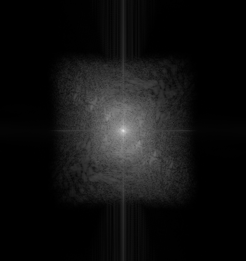
(f) $U(e^{j\boldsymbol{\omega}})$

(g) $V(e^{j\boldsymbol{\omega}})$

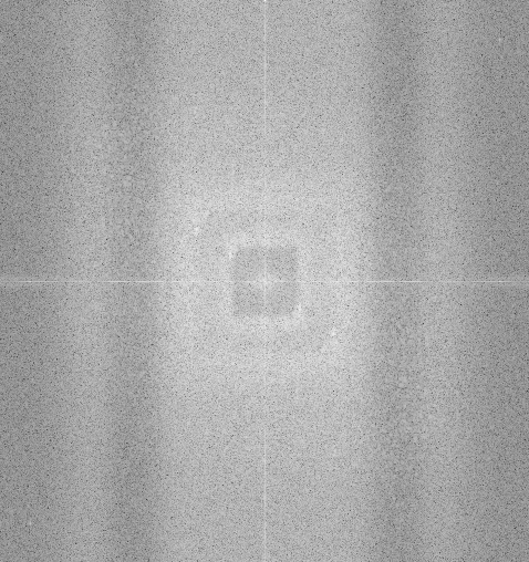
(h) $E(e^{j\boldsymbol{\omega}})$

Figure 3: A fingerprint image and its Fourier spectrum are shown in (a) and (b), respectively. Image (a) is decomposed by G3PD with $\mu_{1}=1$, iteration = 20, level = 5, $\beta_{1}=0.06\,,\beta_{2}=\beta_{3}=\gamma=10^{-3}$ into cartoon (c), texture (d) and noise (e) images. Their respective Fourier spectra are visualized in (f-h). We observe that the Fourier spectra of the component images resemble responses after lowpass, bandpass and highpass filtering. Please note that especially (d) and (g) show that the fingerprint pattern is mostly concentrated in a specific range of frequencies [6].

The oscillation signal corresponding to fingerprint patterns is considered as a sparse and smooth texture which is decomposed by the G3PD model of the original fingerprint image $\boldsymbol{f}$ into three parts satisfying the constraint $\boldsymbol{f}=\boldsymbol{u}+\boldsymbol{v}+\boldsymbol{\epsilon}$ (cf. Figure 3), including: the piecewise-constant image $\boldsymbol{u}$, the texture $\boldsymbol{v}$, and noise $\boldsymbol{\epsilon}$.

In this section, we will analyze how the norms $\mathinner{\!\left\lVert\mathcal{C}\{\boldsymbol{v}\}\right\rVert}_{\ell_{1}}$ and $\mathinner{\!\left\lVert\boldsymbol{v}\right\rVert}_{\ell_{1}}$ in (3) affect on the smoothness and sparsity of the extracted texture which is our main goal for the feature extraction. In order to do that, a closed form of $\boldsymbol{v}$ is found by putting (11) and (14) into (13), letting $\theta=\frac{\beta_{2}}{\beta_{2}+\beta_{3}}$ and the thresholds $T_{1}=\frac{\mu_{1}}{\beta_{2}}$ and $T_{2}=\frac{\mu_{2}}{\beta_{2}+\beta_{3}}$:

$$\boldsymbol{\tilde{v}}~{}=~{}\mathop{\rm Shrink}\Bigg{(}\theta\underbrace{\mathcal{C}^{*}\bigg{\{}\mathop{\rm Shrink}\Big{(}\mathcal{C}\{\boldsymbol{v}\}-\frac{\boldsymbol{\lambda_{2}}}{\beta_{2}}\,,T_{1}\Big{)}+\frac{\boldsymbol{\lambda_{2}}}{\beta_{2}}\bigg{\}}}_{\displaystyle\mathrel{\mathop{\mathchar 58\relax}}=~{}\boldsymbol{v}_{\text{smooth}}~{}\approx~{}\mathop{\rm CST}\big{(}\boldsymbol{v}\,,T_{1}\big{)}}~{}+~{}(1-\theta)\underbrace{\bigg{(}\boldsymbol{f}-\boldsymbol{u}-\boldsymbol{\epsilon}+\frac{\boldsymbol{\lambda_{3}}}{\beta_{3}}\bigg{)}}_{\displaystyle\mathrel{\mathop{\mathchar 58\relax}}=~{}\boldsymbol{v}_{\text{update}}}\,,T_{2}\Bigg{)}.$$ (20)

We see that the estimated texture $\boldsymbol{\tilde{v}}$ contains two shrinkage operators: respectively, the inside and the outside correspond to the smoothness and sparseness terms resulting from $\mathinner{\!\left\lVert\mathcal{C}{\boldsymbol{v}}\right\rVert}_{\ell_{1}}$ and $\mathinner{\!\left\lVert\boldsymbol{v}\right\rVert}_{\ell_{1}}$ in (3). (cf. Figure 4 for the effects of the smoothness and sparseness of $\boldsymbol{v}$ after different numbers of iterations). These effects can be observed in the binarised texture (Figure 4 (f)). The parameter $\theta\in(0\,,1)$ in (20) serves as a regularisation parameter to balance between the smoothing term $\boldsymbol{v}_{\text{smooth}}$ and the updated term $\boldsymbol{v}_{\text{update}}$.

(a) $k=3$

(b) $k=6$

(c) $k=8$

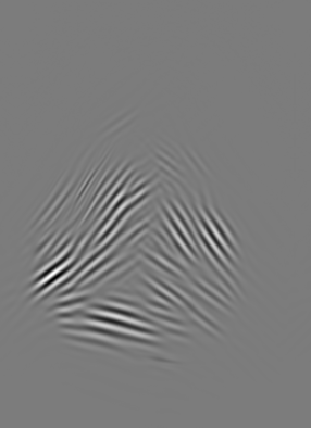
(d) $k=20$

Figure 4: Image (a) depicts the original image where the yellow line indicates the boundary of the ROI estimated by the G3PD method after 20 iterations. The ROI is obtained using morphological operations on the binarized image (f). Images (b-e) show $\boldsymbol{v}_{\text{smooth}}$ in (20), the smoothing term of $\boldsymbol{v}$ and (g-j) visualize the corresponding $\boldsymbol{v}_{\text{update}}$ in (20) after $k$ iterations.

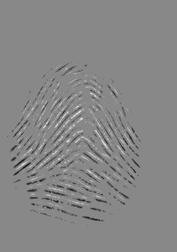
Figure 5: The following comparison illustrates the effect of the smoothness term for $\boldsymbol{v}$ in (1). The first column depicts the $\ell_{1}$ norm of curvelet coefficients, i.e. $\mathinner{\!\left\lVert\mathcal{C}\{\boldsymbol{v}\}\right\rVert}_{\ell_{1}}$ and the second column the $\ell_{1}$ norm of wavelet coefficients, i.e. $\mathinner{\!\left\lVert\mathcal{W}\{\boldsymbol{v}\}\right\rVert}_{\ell_{1}}$ after 50 iterations. Columns 3 and 4 visualize $\boldsymbol{v}$ obtained without smoothness term (no $\mathinner{\!\left\lVert\mathcal{C}\{\boldsymbol{v}\}\right\rVert}_{\ell_{1}}$ in (1)) after 20 and 50 iterations, respectively. The first row shows the texture images $\boldsymbol{v}$, the second row their binarized versions and the third row their plots of convergence rates. The comparison shows that the curvelet based smoothness term leads to a better texture image than the wavelet based one and that convergence without smoothness term is slow and texture tends to be destroyed.

Figure 5 compares the effect of the curvelet smoothness term $\mathinner{\!\left\lVert\mathcal{C}\{\boldsymbol{v}\}\right\rVert}_{\ell_{1}}$ in (1) with a wavelet smoothness term $\mathinner{\!\left\lVert\mathcal{W}\{\boldsymbol{v}\}\right\rVert}_{\ell_{1}}$ and without smoothness measurement. The texture $\boldsymbol{v}$ estimated using $\mathinner{\!\left\lVert\mathcal{W}\{\boldsymbol{v}\}\right\rVert}_{\ell_{1}}$ in (1) is not as good regarding smoothness and sparseness as the texture obtained by the curvelet smoothness term. In order to evaluate the convergence rate of the algorithm, we denote the relative error between successive iterations as

$$\text{Err}^{(n)}_{\boldsymbol{v}}=\frac{\mathinner{\!\left\lVert\boldsymbol{v}^{(n)}-\boldsymbol{v}^{(n-1)}\right\rVert}_{\ell_{2}}}{\mathinner{\!\left\lVert\boldsymbol{v}^{(n-1)}\right\rVert}_{\ell_{2}}}.$$ (21)

In Figure 5, one can see that without smoothness measurement, the convergence rate is slow (cf. 3rd row) and the algorithm tends to eliminate texture (cf. column 3 and 4). Note that for the smoothness measurement $\mathinner{\!\left\lVert\mathcal{C}\{\boldsymbol{v}\}\right\rVert}_{\ell_{1}}$, the proposed method achieves a stable estimated texture $\boldsymbol{v}$ after circa 20 iterations. Hence, the estimated $\boldsymbol{v}$ and its binarisation are almost the same after 20 or 50 iterations (see Figure 4 (f) and 1st column of Figure 5).

2.2 Morphological Operations

Firstly, the smooth and sparse texture $\boldsymbol{v}$ is extracted by the combination of the $\ell_{1}$ norm of its curvelet coefficients and its $\ell_{1}$ norms, simultaneously. Secondly, post-processing as described in [6] is applied to obtain the ROI. More specifically, the morphological operations act only on the non-zero coefficients of the texture image $\boldsymbol{v}$. In other words, this corresponds to a projection of the thresholding value to the parameter $\mu_{2}$ which has been designed to adapt to the intensity of each image by Eq. (18).

3 Evaluation: Benchmark, Protocol and Experimental Results

3.1 Benchmark and Evaluation Metric

The publicly available fingerprint images of the FVC competitions from 2000, 2002 and 2004 are used as benchmark for evaluating segmentation performance. Each competition consists of four databases: three databases are acquired from real fingers and the fourth database of each competition is synthetically generated.

It has recently been shown that real and synthetic fingerprints can be discriminated with very high accuracy using minutiae histograms (MHs) [61]. More specifically, by computing the MH for a minutiae template and then computing the earth mover’s distance (EMD) [62] between the MH of the template and the mean MHs for a set of real and synthetic fingerprints. Classification is simply performed by choosing the class with the smaller EMD.

In total, there are 12 databases and each database contains 880 images (80 for training and 800 for testing). The ground truth segmentation has been manually marked for these 10560 images as described in [6].

Let $N_{1}$ and $N_{2}$ be the width and height of image $\boldsymbol{f}$ in pixels. Let $M_{f}$ be number of pixels which are marked as foreground by human experts and estimated as background by an algorithm (missed/misclassified foreground). Let $M_{b}$ be number of pixels which are marked as background by human experts and estimated as foreground by an algorithm (missed/misclassified background). The average total error per image is defined as

$$Err=\frac{M_{f}+M_{b}}{N_{1}\times N_{2}}.$$ (22)

3.2 Parameter Selection

Parameters for all methods considered in the comparison are selected on the training set of 80 images for each database. More specifically, those parameters are chosen which minimize the segmentation error defined in (22) for the respective training set. Choosing the parameters for each database is appropriate, because the nine databases consisting of real fingerprints have been acquired using nine different sensors and the images of each database have sensor-specific properties. The parameter selection for the FDB [6], GFB [9], HCR [10], MVC [8] and STFT [11] methods are discussed in [6].

Parameters	Description
$N$	the number of iterations in the Algorithm 1.
$\mu_{1}$	the regularised parameter for $\ell_{1}$ norm of curvelet coefficients $\mathcal{C}\{\boldsymbol{v}\}$
	in Eq. (2).
$C$	the adaptive constant in Eq. (18) for the regularised parameter $\mu_{2}$
	in $\ell_{1}$ norm of $\boldsymbol{v}$ in Eq. (2).
$\beta_{1}\,,\beta_{2}\,,\beta_{3}$	the parameters in the augmented Lagrangian function (4).
$\gamma$	the rate of the updated Lagrange multipliers in Eq. (4).
$s$	the window size of the block in the postprocessing step in [6, Eq. (8)].
$t$	a constant for selecting the morphology threshold $T$ in [6, Eq. (8)].
$b$	the number of the neighbouring blocks in [6, Eq. (8)].
$p$	the mirror boundary condition to avoid the boundary effect.

Table 1: Overview over all parameters for the global three-part decomposition (G3PD) method for fingerprint segmentation. Values are reported in Table 2.

FVC	DB	$C$	$\beta_{2}$
2000	1	0.045	0.0005
	2	0.045	0.0100
	3	0.055	0.0010
	4	0.025	0.0010
2002	1	0.020	0.0010
	2	0.035	0.0005
	3	0.070	0.0010
	4	0.020	0.0500
2004	1	0.015	0.1000
	2	0.025	0.0010
	3	0.035	0.0010
	4	0.035	0.0005

Table 2: Overview over the parameters learned on the training set. The other eight parameters are $\mu_{1}=1$, $\beta_{1}=\beta_{3}=\gamma=10^{-3}$, $s=9$, $t=5$, $b=6$ and $p=15$ for all databases.

For the proposed G3PD method, the involved parameters are summarized in Table 1 and the values of the learned parameters are reported in Table 2. In a reasonable amount of time, a number of conceivable parameter combinations were tried on the training set.

For different numbers of iterations, we have applied the following training scheme:

• Firstly, $C$, an adaptive constant for $\mu_{2}$ in (18) to define a threshold for the sparseness of $\boldsymbol{v}$, is trained while fixing the other parameters.

• Secondly, with the obtained $C$, we train the other parameters one by one while fixing the rest.

The two parameters which have the biggest impact on the segmentation performance are the number of iterations $N$ and the constant $C$ in Eq. (18). Therefore, these two parameters have been trained first. In our experiments, the minimum error on the training set averaged over all 12 databases is obtained for $N=4$ iterations. In these practical applications of our proposed model, stopping before convergence leads to better segmentation results which are also influenced by the combination with the morphological operations. For further details and a discussion, see [55].

Note that the solution of $(\boldsymbol{u}\,,\boldsymbol{v}\,,\boldsymbol{\epsilon})$ depends severely on the choices of $(\mu_{1}\,,\mu_{2}\,,\delta)$, as well as the parameters of the optimisation step $(\beta_{1}\,,\beta_{2}\,,\beta_{3}\,,\gamma)$. To achieve a good decomposition in which cartoon, texture and noise are separated is difficult in practice, because there are no models of noise and texture. Fortunately, this paper focuses on the segmentation of fingerprint images for which the texture $\boldsymbol{v}$ is important. After the decomposition, there can still be pattern contents in the cartoon image $\boldsymbol{u}$ and the noise image $\boldsymbol{\epsilon}$ (see Figure 1), but the important aspect is that the texture image $\boldsymbol{v}$ is adequate for segmentation.

The choice of aforementioned parameters balances the amount of pattern in the texture image with the smoothness of the cartoon image. Selecting parameters which increase the smoothness of the cartoon image $\boldsymbol{u}$, also tend to cause the halo effect in the texture image $\boldsymbol{v}$. We observe that especially $\beta_{1}$ influences this trade-off: if $\boldsymbol{u}$ contains only homogeneous regions (cf. Figure 3 (c)), it tends to generate the halo effect on the boundary of fingerprint pattern in $\boldsymbol{v}$ (cf. Figure 3 (d)). Particularly, the halo effect results from the blurred homogeneous region $\boldsymbol{u}$. In order to reduce this effect in $\boldsymbol{v}$, the parameters are chosen such that the algorithm assigns “enough” texture to $\boldsymbol{v}$. Hence, $\boldsymbol{u}$ and $\boldsymbol{\epsilon}$ can contain some partial textures, but this yields better a segmentation performance, cf. [55].

Let us consider the comparison of the proposed model with the standard ROF $\text{TV}-L_{2}$ model [21] and the $\text{TV}-L_{1}$ model [63] for feature decomposition (see Figure 7). For simplicity, let $\lambda_{\text{TV}L_{2}}$ and $\lambda_{\text{TV}L_{1}}$ be the regularisation parameters for $\text{TV}-L_{2}$ and $\text{TV}-L_{1}$, respectively. The ROF $\text{TV}-L_{2}$ model has been introduced by [21] for the purpose of image denoising. The ROF model has been designed to obtain a smooth cartoon image $\boldsymbol{u}$. For fingerprint image segmentation we are interested in a texture image which is as useful as possible in terms of a feature for segmentation. However, the ROF model or the $\text{TV}-L_{1}$ model cannot produce a sparse and smooth texture image from a noisy fingerprint image $\boldsymbol{f}$ no matter how the corresponding parameter is selected. On the one hand, if the ROF model decomposes $\boldsymbol{f}$ into a very smooth cartoon image $\boldsymbol{u}$, than $\boldsymbol{v}$ contains both noise and texture. On the other hand, for a different choice of $\lambda_{\text{TV}L_{2}}$ or $\lambda_{\text{TV}L_{1}}$, $\boldsymbol{v}$ contains mostly noise and $\boldsymbol{u}$ includes texture and large scale objects. In neither of the two situations, $\boldsymbol{u}$ or $\boldsymbol{v}$ is useful as a feature for fingerprint segmentation. A comparison of the G3PD method with $\text{TV}-L_{1}$ and $\text{TV}-L_{2}$ two-part decomposition is shown in Figure 7. Zhang et al. [64] have tried to solve this problem by proposing a locally adaptive two-part decomposition which also takes the orientation of the pattern into account.

In summary, the proposed G3PD method yields a satisfactory performance judged by visual inspection (see Figure 6 for one example from each database) and it outperforms the other methods on ten of twelve databases, see Table 3. This demonstrates the robustness of the G3PD method for fingerprint segmentation.

Figure 6: Segmented fingerprint images and the corresponding texture images by the variational method for FVC2000 (first and second row), FVC2002 (third and fourth row) and FVC2004 (fifth and sixth row). Columns f.l.t.r correspond to DB1 to DB4.

FVC	DB	GFB [9]		HCR [10]		MVC [8]		STFT [11]		FDB [6]		G3PD
2000	1	13.	26	11.	15	10.	01	16.	70	5.	51	5.	69
	2	10.	27	6.	25	12.	31	8.	88	3.	55	4.	10
	3	10.	63	7.	80	7.	45	6.	44	2.	86	2.	68
	4	5.	17	3.	23	9.	74	7.	19	2.	31	2.	06
2002	1	5.	07	3.	71	4.	59	5.	49	2.	39	1.	72
	2	7.	76	5.	72	4.	32	6.	27	2.	91	2.	83
	3	9.	60	4.	71	5.	29	5.	13	3.	35	3.	27
	4	7.	67	6.	85	6.	12	7.	70	4.	49	3.	63
2004	1	5.	00	2.	26	2.	22	2.	65	1.	40	0.	88
	2	11.	18	7.	54	8.	06	9.	89	4.	90	4.	62
	3	8.	37	4.	96	3.	42	9.	35	3.	14	2.	77
	4	5.	96	5.	15	4.	58	5.	18	2.	79	2.	53
Avg.		8.	33	5.	78	6.	51	7.	57	3.	30	3.	06

Table 3: Error rates (average percentage of misclassified pixels averaged over 800 test images per database) computed using the manually marked ground truth segmentation and the estimated segmentation by these methods: a Gabor filter bank (GFB) response based method by Shen et al. [9], a Harris corner response (HCR) based approach by Wu et al. [10], a method by Bazen and Gerez using local grey-level mean, variance and gradient coherence (MVC) as features [8], a method applying short time Fourier transforms (STFT) by Chikkerur et al. [11], the factorized directional bandpass (FDB) [6] and the proposed method based on the G3PD model.

(a) G3PD: $\beta_{1}=0.005$

(b) $\lambda_{\text{TV}L_{2}}=0.1$

(c) $\lambda_{\text{TV}L_{1}}=1$

(d) $\lambda_{\text{TV}L_{2}}=0.02$

(e) $\lambda_{\text{TV}L_{1}}=0.6$

(f) $\lambda_{\text{TV}L_{2}}=0.005$

(g) $\lambda_{\text{TV}L_{1}}=0.1$

Figure 7: A comparison of G3PD with $\text{TV}-L_{2}$ and $\text{TV}-L_{1}$: First row: images f.l.t.r are the original image $\boldsymbol{f}$ and the three-part decomposition by G3PD with $N=50\,,\beta_{1}=0.005$ (see Table 2 for the other parameters): the cartoon image $\boldsymbol{u}$, texture image $\boldsymbol{v}$ and noise image $\boldsymbol{\epsilon}$. The first and second column of rows two to four show images $\boldsymbol{u}$ and $\boldsymbol{v}$, respectively, for $\text{TV}-L_{2}$ two-part decomposition with different values of $\lambda_{\text{TV}L_{2}}$. The third and fourth column show the corresponding images $\boldsymbol{u}$ and $\boldsymbol{v}$ for $TV-L_{1}$ two-part decomposition. The number of iterations for $\text{TV}-L_{2}$ and $\text{TV}-L_{1}$ is $N=350$. Note that for no choice of $\lambda_{\text{TV}L_{2}}$ or $\lambda_{\text{TV}L_{1}}$, $\text{TV}-L_{2}$ or $\text{TV}-L_{1}$ produce a good feature image for segmentation of this noisy fingerprint, while the G3PD model provides a useful texture image $\boldsymbol{v}$ for the segmentation procedure.

4 Conclusions

We have presented a global framework for the fingerprint segmentation problem which is to separate the foreground from background based on texture analysis. We have proposed the G3PD method for three-part decomposition of fingerprint images. The texture pattern is analyzed under the variational approach considering sparsity and smoothness at the same time: with the $\ell_{1}$-norm for sparsity and $\ell_{1}$-norm of curvelet coefficients for smoothness. The resulting texture image is binarised and postprocessed by morphology to obtain the region of interest.

We have proposed a model for three-part decomposition which takes the nature of the texture occurring in real fingerprint images into account. Fingerprint images are characterized by a smooth, curved and oriented pattern which has a sparse representation in certain transform domains.

The G3PD method is somewhat similar in spirit to the FDB method [6] which also takes into account the specific properties of fingerprint patterns. Frequencies occurring in real fingerprints are mostly located in a specific range in the Fourier domain and the corresponding texture is extracted by an elaborate bandpass filtering process involving forward prediction, proximity operator and backward projection. Similarly, the three-part decomposition can be regarded as lowpass, bandpass and highpass filtering of signals corresponding to $\boldsymbol{u}$, $\boldsymbol{v}$ and $\boldsymbol{\epsilon}$, respectively (see images (f-h) in Figure 3). This illustrates the connection between classical bandpass filtering in the Fourier domain and the variational approach.

In conclusion, we have performed an extensive comparison of the G3PD method with five state-of-the-art fingerprint segmentation algorithms on a large benchmark with a variety of different challenges and have found that the G3PD method outperforms its competitors on ten out of twelve database in terms of segmentation accuracy.

We believe that this work paves the way for further research in areas such as latent fingerprint segmentation in which we deal additionally with other kinds of noise like large scale structure noise, or to better deal with the few low-quality examples which still pose problems to the method. We believe that further improvements can be achieved by combining the G3PD method with additional features, e.g. the texture image obtained by the FDB method.

Data Availability Statement

Matlab Implementation of the G3PD Method for Fingerprint Segmentation
http://dx.doi.org/10.6084/m9.figshare.1418020

Benchmark for Fingerprint Segmentation Performance Evaluation
http://dx.doi.org/10.6084/m9.figshare.1294209

Matlab Implementation of the FDB Method for Fingerprint Segmentation
http://dx.doi.org/10.6084/m9.figshare.1294210

FVC databases
http://bias.csr.unibo.it/fvc2000/
http://bias.csr.unibo.it/fvc2002/
http://bias.csr.unibo.it/fvc2004/

References

• [1] C. Gottschlich. Fingerprint growth prediction, image preprocessing and multi-level judgment aggregation. PhD thesis, University of Goettingen, Goettingen, Germany, April 2010.
• [2] C. Gottschlich, P. Mihăilescu, and A. Munk. Robust orientation field estimation and extrapolation using semilocal line sensors. IEEE Transactions on Information Forensics and Security, 4(4):802–811, December 2009.
• [3] C. Gottschlich. Curved-region-based ridge frequency estimation and curved Gabor filters for fingerprint image enhancement. IEEE Transactions on Image Processing, 21(4):2220–2227, April 2012.
• [4] C. Gottschlich and C.-B. Schönlieb. Oriented diffusion filtering for enhancing low-quality fingerprint images. IET Biometrics, 1(2):105–113, June 2012.
• [5] C. Gottschlich, E. Marasco, A.Y. Yang, and B. Cukic. Fingerprint liveness detection based on histograms of invariant gradients. In Proc. IJCB, pages 1–7, Clearwater, FL, USA, September 2014.
• [6] D.H. Thai, S. Huckemann, and C. Gottschlich. Filter design and performance evaluation for fingerprint image segmentation. arXiv:1501.02113 [cs.CV], January 2015.
• [7] T. Goldstein and S. Osher. The split Bregman method for L1-regularized problems. SIAM Journal on Imaging Sciences, 2(2):323–343, April 2009.
• [8] A.M. Bazen and S.H. Gerez. Segmentation of fingerprint images. In Proc. ProRISC, pages 276–280, Veldhoven, The Netherlands, November 2001.
• [9] L.L. Shen, A. Kot, and W.M. Koo. Quality measures of fingerprint images. In Proc. AVBPA, pages 266–271, Halmstad, Sweden, June 2001.
• [10] C. Wu, S. Tulyakov, and V. Govindaraju. Robust point-based feature fingerprint segmentation algorithm. In Proc. ICB 2007, pages 1095–1103, Seoul, Korea, August 2007.
• [11] S. Chikkerur, A. Cartwright, and V. Govindaraju. Fingerprint image enhancement using STFT analysis. Pattern Recognition, 40(1):198–211, 2007.
• [12] N. Otsu. A threshold selection method from gray-level histograms. IEEE Transactions on Systems, Man and Cybernetics, 9(1):62–66, January 1979.
• [13] P. Sahoo, C. Wilkins, and J. Yeager. Threshold selection using Renyi’s entropy. Pattern Recognition, 30(1):71–84, January 1997.
• [14] M.P. de Albuquerque, I.A. Esquef, and A.R.G. Mello. Image thresholding using Tsallis entropy. Pattern Recognition Letters, 25(9):1059–1065, July 2004.
• [15] T.F. Chan and L.A. Vese. Active contours without edges. IEEE Transactions on Image Processing, 10(2):266–277, February 2001.
• [16] X. Bresson, S. Esedoglu, P. Vandergheynst, J.P. Thiran, and S. Osher. Fast global minimization of the active contour/snake model. Journal of Mathematical Imaging and Vision, 28(2):151–167, June 2007.
• [17] T.F. Chan, S. Esedoglu, and M. Nikolova. Algorithms for finding global minimizers of image segmentation and denoising models. SIAM J. Appl. Math., 66(5):1632–1648, February 2012.
• [18] J. Lie, M. Lysaker, and X.C. Tai. A binary level set model and some applications to Mumford-Shah image segmentation. IEEE Transactions on Image Processing, 15(5):1171–1181, May 2006.
• [19] C. Sagiv, N.A. Sochen, and Y.Y. Zeevi. Integrated active contours for texture segmentation. IEEE Transactions on Image Processing, 15(6):1633–1646, June 2006.
• [20] N. Houhou, J.P. Thiran, and X. Bresson. Fast texture segmentation based on semi-local region descriptor and active contour. Numer. Math. Theor. Meth. Appl., 2(4):445–468, November 2009.
• [21] L. Rudin, S. Osher, and E. Fatemi. Nonlinear total variation based noise removal algorithms. Physica D, 60(1-4):259–268, November 1992.
• [22] J.F. Aujol, G. Gilboa, T. Chan, and S. Osher. Structure-texture image decomposition - modeling, algorithms, and parameter selection. International Journal of Computer Vision, 67(1):111–136, April 2006.
• [23] J.F. Aujol, G. Aubert, L.B. Feraud, and A. Chambolle. Image decomposition into a bounded variation component and an oscillating component. Journal of Mathematical Imaging and Vision, 22(1):71–88, January 2005.
• [24] J.F. Aujol and G. Gilboa. Constrained and SNR-based solutions for TV-Hilbert space image denoising. Journal of Mathematical Imaging and Vision, 26(1-2):217–237, November 2006.
• [25] A. Buades, T.M. Le, J.-M. Morel, and L.A. Vese. Fast cartoon + texture image filters. IEEE Transactions on Image Processing, 19(8):1978–1986, August 2010.
• [26] L.A. Vese and S. Osher. Modeling textures with total variation minimization and oscillatory patterns in image processing. Journal of Scientific Computing, 19(1-3):553–572, December 2003.
• [27] G. Aubert and L. Vese. A variational method in image recovery. SIAM J. Numer. Anal, 34(5):1948–1979, October 1997.
• [28] T. Chan, A. Marquina, and P. Mulet. High-order total variation-based image restoration. SIAM Journal on Scientific Computing, 22(2):503–516, July 2000.
• [29] M. Lysaker, A. Lundervold, and X.C. Tai. Noise removal using fourth-order partial differential equation with applications to medical magnetic resonance images in space and time. IEEE Transactions on Image Processing, 12(12):1579–1590, December 2003.
• [30] W.Zhu and T. Chan. Image denoising using mean curvature of image surface. SIAM Journal on Imaging Sciences, 5(1):1–32, January 2012.
• [31] X.C. Tai, J. Hahn, and G.J. Chung. A fast algorithm for Euler’s elastica model using augmented Lagrangian method. SIAM Journal on Imaging Sciences, 4(1):313–344, February 2011.
• [32] K. Papafitsoros and C.B. Schönlieb. A combined first and second order variational approach for image reconstruction. J. Math. Imaging Vis., 48(2):308–338, 2014.
• [33] L. Calatroni, B. Düring, and C.B. Schönlieb. ADI splitting schemes for a fourth-order nonlinear partial differential equation from image processing. DCDS Series A, 34(3):931–957, March 2014.
• [34] G. Song, H. Zhang, and F.J. Hickernell. Reproducing kernel Banach spaces with the L1 norm. Applied and Computational Harmonic Analysis, 34(1):96–116, January 2013.
• [35] W. Yin, S. Osher, D. Goldfarb, and J. Darbon. Bregman iterative algorithms for l1 minimization with applications to compressed sensing. SIAM Journal on Imaging Sciences, 1(1):143–168, March 2008.
• [36] W. Yin, D. Goldfarb, and S. Osher. Image cartoon-texture decomposition and feature selection using the total variation regularization L1 functional. In Proc. VLSM, pages 73–84, Beijing, China, October 2005.
• [37] J. Yang and Y. Zhang. Alternating direction algorithms for l1-problems in compressive sensing. SIAM Journal on Scientific Computing, 33(1):250–278, February 2011.
• [38] E. Candès, M. Wakin, and S. Boyd. Enhancing sparsity by reweighted l1 minimization. J. Fourier Anal. Appl., 14(5):877–905, 2008.
• [39] J.-F. Aujol and A. Chambolle. Dual norms and image decomposition models. International Journal of Computer Vision, 63(1):85–104, June 2005.
• [40] A. Chambolle. An algorithm for total variation minimization and applications. Journal of Mathematical Imaging and Vision, 20(1-2):89–97, January 2004.
• [41] A. Beck and M. Teboulle. A fast iterative shrinkage-thresholding algorithm for linear inverse problems. SIAM Journal on Imaging Sciences, 2(1):183–202, January 2009.
• [42] I. Daubechies, M. Defrise, and C. D. Mol. An iterative thresholding algorithm for linear inverse problems with a sparsity constraint. Communications on Pure and Applied Mathematics, 57(11):1413–1457, August 2004.
• [43] J.B. Dias and M. Figueiredo. A new twist: Two-step iterative shrinkage/thresholding algorithms for image restoration. IEEE Transactions on Image Processing, 16(12):2992–3004, December 2007.
• [44] C. Wu and X. C. Tai. Augmented Lagrangian method, dual methods, and split Bregman iteration for ROF, vectorial TV, and higher order methods. SIAM Journal on Imaging Sciences, 3(3):300–339, July 2010.
• [45] D.L. Donoho and J.M. Johnstone. Ideal spatial adaptation by wavelet shrinkage. Biometrika, 81(3):425–455, August 1994.
• [46] A. Chambolle, R.A. DeVore, N.Y. Lee, and B.J. Lucier. Nonlinear wavelet image processing: variational problems, compression, and noise removal through wavelet shrinkage. IEEE Transactions on Image Processing, 7(3):319–335, March 1998.
• [47] H. Choi and R.G. Baraniuk. Multiple wavelet basis image denoising using Besov ball projections. IEEE Signal Processing Letters, 11(9):717–720, September 2004.
• [48] E. Candès and D. Donoho. New tight frames of curvelets and optimal representations of objects with piecewise singularities. Communications on Pure and Applied Mathematics, 57(2):219–266, February 2004.
• [49] E. Candès, L. Demanet, D. Donoho, and L. Ying. Fast discrete curvelet transforms. Multiscale Model. Simul., 5(3):861–899, September 2006.
• [50] Starck, D.L. Donoho, and E.J. Candès. Astronomical image representation by the curvelet transform. Astron. Astrophys., 398(2):785–800, February 2003.
• [51] J. Ma and G. Plonka. The curvelet transform. IEEE Signal Processing Magazin, 27(2):118–133, March 2010.
• [52] G. Kutyniok and D. Labate, editors. Shearlets. Multiscale Analysis for Multivariate Data. Birkhäuser, Boston, MA, USA, 2012.
• [53] M.N. Do and M. Vetterli. The contourlet transform: An efficient directional multiresolution image representation. IEEE Transactions on Image Processing, 14(12):2091–2106, December 2005.
• [54] M. Unser and D. V. D. Ville. Wavelet steerability and the higher-order Riesz transform. IEEE Transactions on Image Processing, 19(3):636–652, March 2010.
• [55] D.H. Thai. Fourier and Variational Based Approaches for Fingerprint Segmentation. PhD thesis, University of Goettingen, Goettingen, Germany, January 2015.
• [56] K. Frick, P. Marnitz, and A. Munk. Statistical multiresolution Dantzig estimation in imaging: Fundamental concepts and algorithmic framework. Electronic Journal of Statistics, 6:231–268, 2012.
• [57] W. Zhu, X.C. Tai, and T. Chan. Augmented Lagrangian method for a mean curvature based image denoising model. Inverse Problems and Imaging, 7(4):1409 – 1432, November 2013.
• [58] J. C. De Los Reyes and C.B. Schönlieb. Image denoising: Learning noise distribution via PDE-constrained optimisation. Inverse Problems and Imaging, 7(4):1183–1214, November 2013.
• [59] M. Haltmeier and A. Munk. Extreme value analysis of empirical frame coefficients and implications for denoising by soft-thresholding. Applied and Computational Harmonic Analysis, 36(3):434–460, May 2014.
• [60] A. Cohen, I. Daubechies, and J.C. Feauveau. Biorthogonal bases of compactly supported wavelets. Communications on Pure and Applied Mathematics, 45(5):485–560, June 1992.
• [61] C. Gottschlich and S. Huckemann. Separating the real from the synthetic: Minutiae histograms as fingerprints of fingerprints. IET Biometrics, 3(4):291–301, December 2014.
• [62] C. Gottschlich and D. Schuhmacher. The shortlist method for fast computation of the earth mover’s distance and finding optimal solutions to transportation problems. PLoS ONE, 9(10):e110214, October 2014.
• [63] T.F. Chan and S. Esedoglu. Aspects of total variation regularized $\text{L}^{1}$ function approximation. SIAM Journal on Applied Mathematics, 65(5):1817–1837, May 2005.
• [64] J. Zhang, R. Lai, and C.-C.J. Kuo. Adaptive directional total-variation model for latent fingerprint segmentation. IEEE Transactions on Information Forensics and Security, 8(8):1261–1273, August 2013.