UMISS-HEP-2015-02

^† Department of Physics and Astronomy,
    University of Mississippi,
   Lewis Hall, University, Mississippi, 38677 USA

^‡ Department of Physics, Faculty of Science,
   Ain Shams University, Cairo, 11566, Egypt

^§ Center for Fundamental Physics, Zewail City of Science
   and Technology, 6 October City, Giza, Egypt

1 Introduction

The flavor sector of standard model (SM) has many puzzles. A key property of the SM gauge interactions is that they are lepton flavor universal. Evidence for violation of this property would be a clear sign of new physics (NP) beyond the SM. In the search for NP, the second and third generation quarks and leptons could be special because they are comparatively heavier and are expected to be relatively more sensitive to NP. As an example, in certain versions of the two Higgs doublet models (2HDM) the couplings of the new Higgs bosons are proportional to the masses and so NP effects are more pronounced for the heavier generations. Moreover, the constraints on new physics, especially involving the third generation leptons and quarks, are somewhat weaker allowing for larger new physics effects.

Interestingly, there have been some reports of non-universality in the lepton sector from experiments. Recently, the BaBar Collaboration with their full data sample has reported the following measurements [1, 2]:

$$R(D) \equiv \frac{{\cal B}(\bar{B}\to D^{+}\tau^{-}{\bar{\nu}}_{\tau})}{{\cal B}(\bar{B}\to D^{+}\ell^{-}{\bar{\nu}}_{\ell})}=0.440\pm 0.058\pm 0.042~{},$$

$$R(D^{*}) \equiv \frac{{\cal B}(\bar{B}\to D^{*+}\tau^{-}{\bar{\nu}}_{\tau})}{{\cal B}(\bar{B}\to D^{*+}\ell^{-}{\bar{\nu}}_{\ell})}=0.332\pm 0.024\pm 0.018~{},$$ (1)

where $\ell=e,\mu$. The SM predictions are $R(D)=0.297\pm 0.017$ and $R(D^{*})=0.252\pm 0.003$ [1, 3], which deviate from the BaBar measurements by 2$\sigma$ and 2.7$\sigma$, respectively. (The BaBar Collaboration itself reported a 3.4$\sigma$ deviation from SM when the two measurements of Eq. (1) are taken together.) This measurement of lepton flavor non-universality, referred to as the $R(D^{(*)})$ puzzles, may be providing a hint of the new physics (NP) believed to exist beyond the SM. There have been numerous analyses examining NP explanations of the $R(D^{(*)})$ measurements [4, 5].

In another measurement the LHCb Collaboration recently measured the ratio of decay rates for $B^{+}\to K^{+}\ell^{+}\ell^{-}$ ($\ell=e,\mu$) in the dilepton invariant mass-squared range 1 GeV² $\leq q^{2}\leq 6$ GeV² [6]. They found

$$R_{K}\equiv\frac{{\cal B}(B^{+}\to K^{+}\mu^{+}\mu^{-})}{{\cal B}(B^{+}\to K^{+}e^{+}e^{-})}=0.745^{+0.090}_{-0.074}~{}{\rm(stat)}\pm 0.036~{}{\rm(syst)}~{},$$ (2)

is a $2.6\sigma$ difference from the SM prediction of $R_{K}=1\pm O(10^{-4})$ [7]. In addition, we note that the three-body decay $B^{0}\to K^{*}\mu^{+}\mu^{-}$ by itself offers a large number of observables in the kinematic and angular distributions of the final-state particles, and it has been argued that some of these distributions are less affected by hadronic uncertainties [8]. Interestingly, the measurement of one of these observables shows a deviation from the SM prediction [9]. However, the situation is not clear whether this anomaly is truly a first sign of new physics [10].

The tau neutrino, $\nu_{\tau}$, was discovered by the DONuT experiment [11] which measured the charged-current (CC) interaction cross section of the tau neutrino. The DONuT central-value results for the $\nu_{\tau}$ scattering cross section show deviation from the standard model predictions by about 40% but with large experimental errors; thus, the measurements are consistent with the standard model. The third generation lepton has been explored relatively less than the other two generations and in particular there has not been much investigation of $\nu_{\tau}$ properties. One of the predictions of the Standard Model (SM) is that gauge bosons couple to the three generations of leptons universally. A careful test of this prediction is very important and observation of non-universality in the interactions of the lepton families would be an important discovery.

In previous publications we considered new physics in $\nu_{\tau}$ scattering for quasi-exclusive, resonant and DIS scattering [12]. In those papers we were more focused on the error in the extraction of neutrino mixing angles in presence of new physics. In this paper we focus on observables that may be measured at a $\nu_{\tau}$ scattering experiment. There is a proposed Search for Hidden Particles (SHiP) experiment at CERN [13] which is expected to have a large sample of tau neutrinos which could be used to probe new physics in $\nu_{\tau}$ scattering. In our previous work we did not include new physics tensor interactions which we consider in this work. In this work we will be interested at neutrino energies where the DIS component of the scattering process is dominant.

We start with an effective Hamiltonian description of new physics operators. We fix the constraints on the couplings from charged current $\tau$ decays. We consider the decays $\tau\to\pi\nu_{\tau}$ and $\tau\to\pi\pi\nu_{\tau}$ which are well measured. We finally consider an explicit leptoquark model where both scalar and tensor interactions, with relations between the couplings of the two interactions, are present.

The paper is organized in the following manner. In sec. 2 we introduce the effective Lagrangian to parametrize the NP operators, describe the formalism of the decay process and introduce the relevant observables. In sec.3 we present our results and in sec.4 we present our conclusions. We collect some of our equations in Appendices (A, B).

2 Formalism

In the presence of NP, the effective Hamiltonian for the scattering process $\nu_{\tau}+N\to\tau+X$ can be written in the form [14],

$${\cal{H}}_{eff} = \frac{4G_{F}V_{ud}}{\sqrt{2}}\Big{[}(1+V_{L})\,[\bar{u}\gamma_{\mu}P_{L}d]~{}[\bar{l}\gamma^{\mu}P_{L}\nu_{l}]\,+V_{R}\,[\bar{u}\gamma^{\mu}P_{R}d]~{}[\bar{l}\gamma_{\mu}P_{L}\nu_{l}]$$ (3)

$$\,+S_{L}\,[\bar{u}P_{L}d]\,[\bar{l}P_{L}\nu_{l}]\,+S_{R}\,~{}[\bar{u}P_{R}d]\,~{}[\bar{l}P_{L}\nu_{l}]\,+T_{L}\,[\bar{u}\sigma^{\mu\nu}P_{L}d]\,~{}[\bar{l}\sigma_{\mu\nu}P_{L}\nu_{l}]\Big{]}\,,$$

where $G_{F}=1.1663787(6)\times 10^{-5}GeV^{-2}$ is the Fermi coupling constant, $V_{ud}$ is the Cabibbo-Kobayashi-Maskawa (CKM) matrix element, $P_{L,R}=(1\mp\gamma_{5})/2$ are the projectors of negative/positive chiralities. We use $\sigma_{\mu\nu}=i[\gamma_{\mu},\gamma_{\nu}]/2$ and assume the neutrino to be always left chiral. To introduce non-universality the NP couplings are in general different for different lepton flavors. We assume the NP effect is mainly through the $\tau$ lepton. The effective Hamiltonian involves the quarks of the first generations only. It is possible that the quarks of the other generations will also be affected by new physics. We will not assume any connection between new physics for the different generations of quarks. The SM effective Hamiltonian corresponds to $g_{L}=g_{R}=g_{S}=g_{P}=0$.

The Hamiltonian in the presence of only scalar and tensor operators can be written as,

$${\cal{H}}_{\rm eff}=\frac{G_{F}V_{ud}}{\sqrt{2}}\left[\bar{u}(A_{S}+B_{S}\gamma_{5})d\;\bar{l}(1-\gamma_{5})\nu_{l}+T_{L}\;\bar{u}\sigma^{\mu\nu}(1-\gamma_{5})d\;\bar{l}\sigma_{\mu\nu}(1-\gamma_{5})\nu_{l}\right],$$ (4)

where $A_{S}=S_{R}+S_{L}$ and $B_{S}=S_{R}-S_{L}$ with $S_{L}$ and $S_{R}$ are the left and right handed scalar couplings and $T_{L}$ is the tensor coupling.

We will first employ a model independent approach and treat the scalar and tensor couplings one at a time. Since, in many realistic models both the scalar and tensor couplings may be present, we will consider an explicit leptoquark model where both the scalar and tensor couplings are present.

The Hamiltonian in the presence of only $V\pm A$ operators was considered in our previous work [12]. There the effective Hamiltonian was written in terms of a $W^{\prime}$ model, which could arise in extensions of the SM [15], as

$${\cal{L}} = \frac{g}{\sqrt{2}}V_{f^{\prime}f}\bar{f}^{\prime}\gamma^{\mu}(g^{f^{\prime}f}_{L}P_{L}+g^{f^{\prime}f}_{R}P_{R})fW^{\prime}_{\mu}+~{}h.c.$$ (5)

Integrating out the $W^{\prime}$ leads to

$${\cal{L}} = \frac{g^{2}}{2M_{W}^{2}}V_{f^{\prime}f}\left[\bar{f}^{\prime}\gamma^{\mu}\left(\frac{M_{W}^{2}}{M_{W^{\prime}}^{2}}g^{f^{\prime}f}_{L}P_{L}+\frac{M_{W}^{2}}{M_{W^{\prime}}^{2}}g^{f^{\prime}f}_{R}P_{R}\right)f\right]\left[g^{l,\nu_{l}}\bar{l}\gamma_{\mu}P_{L}\nu_{l}\right]+~{}h.c.,$$

$${\cal{L}} = \frac{4G_{F}V_{f^{\prime}f}}{\sqrt{2}}\left[\bar{f}^{\prime}\gamma^{\mu}\left(\frac{M_{W}^{2}}{M_{W^{\prime}}^{2}}g^{f^{\prime}f}_{L}P_{L}+\frac{M_{W}^{2}}{M_{W^{\prime}}^{2}}g^{f^{\prime}f}_{R}P_{R}\right)f\right]\left[g_{\nu_{l},l}\bar{l}\gamma_{\mu}P_{L}\nu_{l}\right]+~{}h.c.$$

Comparing Eq. LABEL:intwprime with Eq. 3 we have the following relations

$$V_{L} = \frac{M_{W}^{2}}{M_{W^{\prime}}^{2}}g^{f^{\prime}f}_{L}g^{l,\nu_{l}},$$

$$V_{R} = \frac{M_{W}^{2}}{M_{W^{\prime}}^{2}}g^{f^{\prime}f}_{R}g^{l,\nu_{l}}.$$ (7)

2.1 Deep Inelastic Neutrino Nucleon Scattering

In this section we discuss Deep Inelastic Neutrino Nucleon Scattering with the various types of interactions.

2.1.1 Scalar and Tensor Interactions

In this section, we first present the total and differential cross sections for the deep inelastic scattering (DIS) process

$$\nu_{\tau}+N\to\tau+X,\;\;\;\nu_{\mu}+N\to\mu+X,$$ (8)

with scalar and tensor interactions. The total differential cross section is written in terms of contributions from the standard model, scalar and tensor operators and cross terms as follows

$$\frac{d\sigma_{\rm tot}}{dxdy}=\frac{d\sigma_{\rm SM}}{dxdy}+\frac{d\sigma_{\rm S}}{dxdy}+\frac{d\sigma_{\rm T}}{dxdy}+\frac{d\sigma_{\rm SM,ST}}{dxdy}+\frac{d\sigma_{\rm S,T}}{dxdy}.$$ (9)

The differential cross section is given in terms of the cross section amplitude as follows

$$\frac{d\sigma}{dxdy}=\frac{1}{32\pi ME_{\nu}}\int\frac{d\xi}{\xi}f(\xi)|\bar{\mathcal{M}}(\xi)|^{2}\delta(\xi-x).$$ (10)

Here, $p_{q}^{\mu}=\xi p^{\mu}$ is the four-momentum of the scattered quark, $p^{\mu}$ is the target nucleon momentum, and $\xi$ is its momentum fraction. $f(\xi)$ is the the parton distribution function (PDF) inside a nucleon and $E_{\nu}$ is the incoming neutrino energy. In the deep inelastic scattering we calculate the differential cross section with respect to the scaling variables which are defined as follows

$$x = \frac{q^{2}}{2\,\nu},$$

$$y = \frac{\nu}{ME_{\nu}},$$ (11)

where $x$ is the Bjorken variable and $y$ is the inelasticity with $q$ being the four-momentum transfer of the leptonic probe and

$$\nu=-p\cdot q=M(E_{\nu}-E_{\ell}).$$ (12)

The physical regions for $x$ and $y$ are obtained by Albright and Jarlskog [16, 17]

$$\frac{m_{\ell}^{2}}{2M(E_{\nu}-m_{\ell})}\leq x\leq 1,$$ (13)

and

$$A-B\leq y\leq A+B,$$ (14)

where

$$A=\frac{1}{2}\left(1-\frac{m_{\ell}^{2}}{2ME_{\nu}x}-\frac{m_{\ell}^{2}}{2E_{\nu}^{2}}\right)\bigg{/}\left(1+\frac{xM}{2E_{\nu}}\right),$$ (15)

$$B=\frac{1}{2}\left[\left(1-\frac{m_{\ell}^{2}}{2ME_{\nu}x}\right)^{2}-\frac{m_{\ell}^{2}}{E_{\nu}^{2}}\,\right]^{\frac{1}{2}}\Bigg{/}\left(1+\frac{xM}{2E_{\nu}}\right).$$ (16)

The terms in Eq. 9 are given as

$$\frac{d\sigma_{\rm SM}}{dxdy} = \frac{G_{F}^{2}ME_{\nu}}{\pi}\left(y(xy+\frac{m_{\ell}^{2}}{2ME_{\nu}})F_{1}+(1-y-\frac{Mxy}{2E_{\nu}}-\frac{m_{\ell}^{2}}{4E_{\nu}^{2}})F_{2}\right.$$

$$\left.+(xy(1-\frac{y}{2})-y\frac{m_{\ell}^{2}}{4ME_{\nu}})F_{3}-\frac{m_{\ell}^{2}}{2ME_{\nu}}F_{5}\right),$$

$$\frac{d\sigma_{\rm S}}{dxdy} = \frac{G_{F}^{2}ME_{\nu}}{4\pi}(A_{S}^{2}+B_{S}^{2})y(xy+\frac{m_{\ell}^{2}}{2ME_{\nu}})F_{1},$$

$$\frac{d\sigma_{\rm T}}{dxdy} = \frac{8G_{F}^{2}ME_{\nu}}{\pi}T_{L}^{2}\left(y(xy+\frac{m_{\ell}^{2}}{2ME_{\nu}})F_{1}+2(1-y-\frac{Mxy}{4E_{\nu}}-\frac{m_{\ell}^{2}}{8E_{\nu}^{2}})F_{2}-\frac{m_{\ell}^{2}}{ME_{\nu}}F_{5}\right),$$

$$\frac{d\sigma_{\rm SM,ST}}{dxdy} = 0,$$

$$\frac{d\sigma_{\rm S,T}}{dxdy} = \frac{2G_{F}^{2}ME_{\nu}}{\pi}T_{L}(B_{S}-A_{S})\left(xy(1-\frac{y}{2})-y\frac{m_{\ell}^{2}}{4ME_{\nu}}\right)F_{3}.$$ (17)

The functions $F_{i}$ are given as

$$F_{1} = \sum_{q,\bar{q}}f_{q,\bar{q}}(\xi,Q^{2})V^{2}_{q,q^{\prime}},$$

$$F_{2} = 2\sum_{q,\bar{q}}\xi f_{q,\bar{q}}(\xi,Q^{2})V^{2}_{q,q^{\prime}},$$

$$F_{3} = 2\sum_{q}f_{q}(\xi,Q^{2})V^{2}_{q,q^{\prime}}-2\sum_{\bar{q}}f_{\bar{q}}(\xi,Q^{2})V^{2}_{\bar{q},\bar{q}^{\prime}},$$

$$F_{5} = 2\sum_{q,\bar{q}}f_{q,\bar{q}}(\xi,Q^{2})V^{2}_{q,q^{\prime}},$$ (18)

where $f_{q}$ and $f_{\bar{q}}$ are the parton distribution functions inside a nucleon, $V_{q,q^{\prime}}$ is the CKM matrix element, and $Q^{2}=-q^{2}$.

One can write the differential cross sections above in terms of different variables $(t,\nu)$ using Eq. 11 and the transformation [17],

$$\frac{d\sigma}{dxdy}=2ME_{\nu}\nu\frac{d\sigma}{dq^{2}d\nu}.$$ (19)

In the new variables, the differential cross sections can be written in the form

$$\frac{d\sigma_{\rm SM}}{dq^{2}d\nu} = \frac{G_{F}^{2}}{8\pi ME_{\nu}^{2}}\left(2(q^{2}+m_{\ell}^{2})W_{1}+\left(4E_{\nu}(E_{\nu}-\frac{\nu}{M})-(q^{2}+m_{\ell}^{2})\right)W_{2}\right.$$

$$\left.+\frac{1}{M^{2}}(2ME_{\nu}q^{2}-\nu(q^{2}+m_{\ell}^{2}))W_{3}-\frac{2m^{2}_{\ell}E_{\nu}}{M}W_{5}\right),$$

$$\frac{d\sigma_{\rm S}}{dq^{2}d\nu} = \frac{G_{F}^{2}}{16\pi ME_{\nu}^{2}}(A_{S}^{2}+B_{S}^{2})(m_{\ell}^{2}+q^{2})W_{1},$$

$$\frac{d\sigma_{\rm T}}{dq^{2}d\nu} = \frac{G_{F}^{2}}{\pi ME_{\nu}^{2}}T_{L}^{2}\left(2(m_{\ell}^{2}+q^{2})W_{1}+(8E_{\nu}^{2}-(m_{\ell}^{2}+q^{2})-\frac{8E_{\nu}\nu}{M})W_{2}-\frac{4m_{\ell}^{2}E_{\nu}}{M}W_{5}\right),$$

$$\frac{d\sigma_{\rm S,T}}{dq^{2}d\nu} = \frac{G_{F}^{2}}{4\pi M^{3}E_{\nu}^{2}}T_{L}(B_{S}-A_{S})(2E_{\nu}Mq^{2}-(m_{\ell}^{2}+q^{2})\nu)W_{3},$$ (20)

where the (time-reversal invariant) structure functions are [17]

$$W_{1}(q^{2},\nu) = \frac{F_{1}(x)}{M},$$

$$W_{2}(q^{2},\nu) = \frac{MF_{2}(x)}{\nu},$$

$$W_{3}(q^{2},\nu) = \frac{MF_{3}(x)}{\nu},$$

$$W_{5}(q^{2},\nu) = \frac{MF_{5}(x)}{\nu}.$$ (21)

We also define some Lorentz invariant variables in terms of the four-momenta of incoming neutrino $(k)$, target nucleon $(p)$ and the produced charged lepton $(k^{\prime})$ in the laboratory frame

$$Q^{2}=-q^{2}=-t,$$ (22)

$$W^{2}=(p+q)^{2}.$$ (23)

$Q^{2}$ is the magnitude of the momentum transfer and $W$ is the hadronic invariant mass. The physical regions of these variables are given by [22]

$$W_{\rm cut}\leq W\leq\sqrt{s}-m_{\ell},$$ (24)

in the DIS region with $W_{\rm cut}=1.4-1.6$ GeV, and

$$Q^{2}_{-}(W)\leq Q^{2}\leq Q^{2}_{+}(W),$$ (25)

where $s=(k+p)^{2}$ and

$$Q^{2}_{\pm}(W)=\frac{s-M^{2}}{2}(1\pm\bar{\beta})-\frac{1}{2}\left[W^{2}+m^{2}_{\ell}-\frac{M^{2}}{s}\left(W^{2}-m^{2}_{\ell}\right)\right],$$ (26)

with $\bar{\beta}=\lambda^{\frac{1}{2}}\left(1,m^{2}_{\ell}/s,W^{2}/s\right)$ and $\lambda(a,b,c)=a^{2}+b^{2}+c^{2}-2(ab+bc+ca)$. In the lab frame, $s=M^{2}+2ME_{\nu}$.

2.1.2 Explicit Leptoquark Model

Here we will discuss an explicit leptoquark model. Many extensions of the SM, motivated by a unified description of quarks and leptons, predict the existence of new scalar and vector bosons, called leptoquarks, which decay into a quark and a lepton. These particles carry non-zero baryon and lepton numbers, color and fractional electric charges. The most general dimension four $SU(3)_{c}\times SU(2)_{L}\times U(1)_{Y}$ invariant Lagrangian of leptoquarks satisfying baryon and lepton number conservation was considered in Ref [18]. As the tensor operators in the effective Lagrangian get contributions only from scalar leptoquarks, we will focus only on scalar leptoquarks and consider the case where the leptoquark is a weak doublet or a weak singlet. The weak doublet leptoquark, $R_{2}$ has the quantum numbers $(3,2,-7/6)$ under $SU(3)_{c}\times SU(2)_{L}\times U(1)_{Y}$ while the singlet leptoquark $S_{1}$ has the quantum numbers $(\bar{3},1,-1/3)$.

The interaction Lagrangian that induces contributions to $\nu_{\tau}+N\to\tau+X$ process is [19, 20]

$$\mathcal{L}_{2}^{\rm LQ} = \left(g_{2L}^{ij}\overline{u}_{iR}L_{jL}+g_{2R}^{ij}\overline{Q}_{jL}i\sigma_{2}l_{iR}\right)R_{2},$$

$$\mathcal{L}_{0}^{\rm LQ} = \left(g_{1L}^{ij},\overline{Q}_{iL}^{c}i\sigma_{2}L_{jL}+g_{1R}^{ij},\overline{u}_{iR}^{c}\ell_{jR}\right)S_{1},\$$ (27)

where $Q_{i}$ and $L_{j}$ are the left-handed quark and lepton $SU(2)_{L}$ doublets respectively, while $u_{iR}$, $d_{iR}$ and $\ell_{jR}$ are the right-handed up, down quark and charged lepton $SU(2)_{L}$ singlets. Indices $i$ and $j$ denote the generations of quarks and leptons and $\psi^{c}=C\overline{\psi}^{T}=C\gamma^{0}\psi^{*}$ is a charge-conjugated fermion field. The fermion fields are given in the gauge eigenstate basis and one should make the transformation to the mass basis. Assuming the quark mixing matrices to be hierarchical, and considering only the leading contribution we can ignore the effect of mixing.

The couplings in Eq. 27 can be constrained from $\tau$ decays. Because of the doublet nature of $R_{2}$ there will be additional term like $\bar{\tau}\tau\bar{q}q$ which do not contribute to $\tau$ decays. They will contribute to tau pair production but are much smaller than the SM production and hence do not add any new constraints.

After performing the Fierz transformations, one finds the general Wilson coefficients at the leptoquark mass scale contributing to the $\nu_{\tau}+N\to\tau+X$ process:

$$S_{L} = {1\over 2\sqrt{2}G_{F}V_{ud}}\left[-{g_{1L}^{13}g_{1R}^{13*}\over 2M_{S_{1}}^{2}}-{g_{2L}^{13}g_{2R}^{13*}\over 2M_{R_{2}}^{2}}\right],$$

$$T_{L} = {1\over 2\sqrt{2}G_{F}V_{ud}}\left[{g_{1L}^{13}g_{1R}^{13*}\over 8M_{S_{1}}^{2}}-{g_{2L}^{13}g_{2R}^{13*}\over 8M_{R_{2}}^{2}}\right].\,$$ (28)

It is clear from Eq. 2.1.2 that the combination from the weak singlet leptoquark and the weak doublet can add constructively or destructively to the Wilson’s coefficients of the scalar and tensor operators in the effective Hamiltonian. In this section we will also consider the possibilities where both the scalar and the tensor operators are present and are of similar sizes. In the most general case both the singlet and doublet leptoquarks are present and so both the scalar and tensor operators appear in the effective Hamiltonian. As there is limited experimental information, including both the singlet and the doublet leptoquarks will allow us more flexibility in fitting for the Wilson’s coefficients but this will come with the price of less precise predictions for the various observables. We can, therefore, consider the simpler cases when only a singlet or a doublet leptoquark is present. In these cases, from Eq. 2.1.2 the coefficients of scalar operators and the tensor operators are related. One can then consider the two cases:

Case. (a): In this case only the weak doublet scalar leptoquark $R_{2}$ is present. In this case the Wilson’s coefficients are

$$S_{L} = {1\over 2\sqrt{2}G_{F}V_{ud}}\left[-{g_{2L}^{13}g_{2R}^{13*}\over 2M_{R_{2}}^{2}}\right],$$

$$T_{L} = {1\over 2\sqrt{2}G_{F}V_{ud}}\left[-{g_{2L}^{13}g_{2R}^{13*}\over 8M_{R_{2}}^{2}}\right].\$$ (29)

Case. (b): In this case only the singlet leptoquark is present and the relevant Wilson’s coefficients are

$$S_{L} = {1\over 2\sqrt{2}G_{F}V_{ud}}\left[-{g_{1L}^{13}g_{1R}^{13*}\over 2M_{S_{1}}^{2}}\right],$$

$$T_{L} = {1\over 2\sqrt{2}G_{F}V_{ud}}\left[{g_{1L}^{13}g_{1R}^{13*}\over 8M_{S_{1}}^{2}}\right].\,$$ (30)

In the $(\bar{3},1,-1/3)$ case, proton decay can occur in presence of an additional leptoquark couplings to two quarks. The proton decay only constraints the leptoquark mass and the product of this additional coupling with the coupling considered here and so we can choose to turn the proton decay constraint as a constraint on the additional coupling involving the two quarks. Moreover, the relevant couplings for the considered processes involve the third generation and so proton decay constraints do not apply in general to these couplings. Also note the proton cannot kinematically decay to a $\tau$.

The relations in Eqs. (2.1.2, 2.1.2) are valid at the leptoquark mass scale. We have to run them down to the $\tau$ mass scale using the scale dependence of the scalar and tensor currents at leading logarithm approximation

$$S_{L}(m_{\tau}) = \left[\alpha_{s}(m_{t})\over\alpha_{s}(m_{\tau})\right]^{\gamma_{S}\over 2\beta_{0}^{(5)}}\left[\alpha_{s}(m_{\rm LQ})\over\alpha_{s}(m_{t})\right]^{\gamma_{S}\over 2\beta_{0}^{(6)}}S_{L}(m_{\rm LQ}),$$

$$T_{L}(m_{\tau}) = \left[\alpha_{s}(m_{t})\over\alpha_{s}(m_{\tau})\right]^{\gamma_{T}\over 2\beta_{0}^{(5)}}\left[\alpha_{s}(m_{\rm LQ})\over\alpha_{s}(m_{t})\right]^{\gamma_{T}\over 2\beta_{0}^{(6)}}T_{L}(m_{\rm LQ})\,,$$ (31)

where the anomalous dimensions of the scalar and tensor operators are $\gamma_{S}=-6C_{F}=-8$, $\gamma_{T}=2C_{F}=8/3$ respectively. Further, the beta function, $\beta_{0}^{(f)}=11-2n_{f}/3$ [21, 23, 24] and $n_{f}$ is the number of active quark flavors. One can use the equations above to run down the couplings from a chosen value of $m_{\rm LQ}$ to the tau mass, $m_{\tau}$.

In the presence of only one type of leptoquark, singlet or doublet state, one finds that the scalar $S_{L}$ and tensor $T_{L}$ Wilson coefficients are related to each other at the scale of leptoquark mass, $S_{L}(m_{\rm LQ})=\pm 4T_{L}(m_{\rm LQ})$.

2.1.3 $V\pm A$ interactions

The DIS differential cross section in the presence of V$\pm$A operators with respect to the variables $(x,y)$ is given in [12]. Here we write it in terms of the momentum transfer, using Eq. 19 as follows

$$\frac{d\sigma_{\rm SM+(V\pm A)}}{dq^{2}d\nu} = \frac{G_{F}^{2}}{8\pi ME_{\nu}^{2}}\left(\left(|a^{\prime}|^{2}+|b^{\prime}|^{2}\right)(m_{\ell}^{2}+q^{2})W_{1}\right.$$

$$\left.+\frac{1}{2M}\left(|a^{\prime}|^{2}+|b^{\prime}|^{2}\right)(4E_{\nu}^{2}M-4E_{\nu}\nu-M(m_{\ell}^{2}+q^{2}))W_{2}\right.$$

$$\left.+\frac{1}{M^{2}}Re[a^{\prime}b^{\prime*}](2E_{\nu}Mq^{2}-\nu(m_{\ell}^{2}+q^{2}))W_{3}-\frac{1}{M}\left(|a^{\prime}|^{2}+|b^{\prime}|^{2}\right)m_{\ell}^{2}E_{\nu}W_{5}\right),$$

where the definitions are

$$a^{\prime} = 1+{\gamma}^{\rho},$$

$$b^{\prime} = 1+{\gamma}^{\kappa},$$

$${\gamma}^{\rho} = V_{L}+V_{R},$$

$${\gamma}^{\kappa} = V_{L}-V_{R}.$$ (33)

3 Constraints on NP couplings

The scalar couplings $S_{L}$ and $S_{R}$ can be constrained by the tau decay channel $\tau^{-}(k_{1})\rightarrow\nu_{\tau}(k_{2})+\pi^{-}(q)$, while the tensor coupling $T_{L}$ can be constrained by the three-body decay channel $\tau(p)\to\pi^{-}(p_{1})+\pi^{0}(p_{2})+\nu_{\tau}(p_{3})$. In this section we will discuss the constraints.

3.1 $\tau^{-}(k_{1})\rightarrow\nu_{\tau}(k_{2})+\pi^{-}(q)$

The hadronic current of the bound state $\pi$ can be parametrized as

$$\langle 0|\bar{d}\gamma^{\mu}(1-\gamma^{5})u|\pi(q)\rangle=-i\sqrt{2}f_{\pi}q^{\mu},$$ (34)

where $f_{\pi}=(92.4\pm 0.1\pm 0.3)$ MeV [25] is the pion decay constant. The SM decay rate is

$$\Gamma_{\rm SM}^{\pi}=\frac{1}{8\pi}G_{F}^{2}|V_{ud}|^{2}f_{\pi}^{2}m_{\tau}^{3}\left(1-\frac{m_{\pi}^{2}}{m_{\tau}^{2}}\right)^{2}\delta_{\tau/\pi}\,.$$ (35)

Here $\delta_{\tau/\pi}=1.0016\pm 0.0014$ [26] is the radiative correction. Further, the SM branching ratio can also be expressed as [27]

$$Br^{SM}_{\tau^{-}\to\pi^{-}\nu_{\tau}} = 0.607Br(\tau^{-}\to\nu_{\tau}e^{-}\bar{\nu}_{e})=10.82\pm 0.02\%\,,$$ (36)

while the measured $Br(\tau^{-}\to\pi^{-}\nu_{\tau})_{exp}=(10.91\pm 0.07)\%$ [25]. In the presence of a scalar state, the decay rate is

$$\Gamma_{\rm S}^{\pi}=\frac{1}{8\pi}G_{F}^{2}|V_{ud}|^{2}B_{S}^{2}f_{\pi}^{2}m_{\pi}^{2}m_{\tau}\left(1-\frac{m_{\pi}^{2}}{m_{\tau}^{2}}\right)^{2},$$ (37)

where

$$\langle 0|\bar{d}(A_{S}-B_{S}\gamma^{5})u|\pi(q)\rangle=i\sqrt{2}f_{\pi}m_{\pi}B_{S}.$$ (38)

In order to obtain the scalar hadronic current above, we have multiplied the SM hadronic current (34) by the sum and difference of the quark momenta and used the equation of motion - see Appendix (B). The total branching ratio can be written as follows

$$BR_{\rm tot}^{\pi}=BR_{\rm SM}^{\pi}\left(1+(r_{\rm S}^{\pi})^{2}\right),$$ (39)

where

$$(r_{\rm S}^{\pi})^{2} = \frac{BR_{\rm S}^{\pi}}{BR_{\rm SM}^{\pi}},$$ (40)

with

$$r_{\rm S}^{\pi}=\frac{B_{S}m_{\pi}}{m_{\tau}}.$$ (41)

Note, the interference term of the SM and the scalar NP term vanishes.

The allowed region of the couplings are given in the contour plot Fig. 1 for the measured $\tau^{-}\to\pi^{-}\nu_{\tau}$ within the $2\sigma$ level. We consider theoretical uncertainty within the $1\sigma$ level. First, we assume both couplings, $S_{L,R}$, are present and take the couplings to be real. Next we assume the couplings are complex and take one coupling at a time, as shown in Fig. 2.

Figure 1: The constraints on the scalar couplings $S_{L,R}$. The colored region is allowed. The constraint is from $\tau^{-}\rightarrow\pi^{-}\nu_{\tau}$. We treat $S_{L}$ and $S_{R}$ as real couplings.

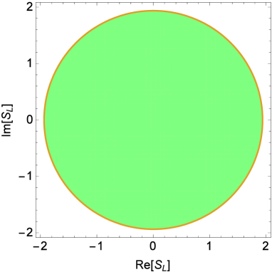
Figure 2: The constraints on the scalar couplings $S_{L,R}$. The colored region is allowed. The constraint is from $\tau^{-}\rightarrow\pi^{-}\nu_{\tau}$. Left panel: we take $S_{R}=0$ and treat $S_{L}$ as a complex coupling. Right panel: we take $S_{L}=0$ and treat $S_{R}$ as a complex coupling.

3.2 $\tau(p)\to\pi^{-}(p_{1})+\pi^{0}(p_{2})+\nu_{\tau}(p_{3})$

Here we consider two-pion decays of $\tau$. The process is

$$\tau(p)\to\nu_{\tau}(p_{3})+\pi^{-}(p_{1})+\pi^{0}(p_{2}).$$ (42)

The SM and NP amplitudes are

$$M_{SM}=\frac{-iG_{F}V_{ud}}{\sqrt{2}}\langle\pi^{-}\pi^{0}|\bar{d}\gamma^{\mu}(1-\gamma^{5})u|0\rangle\bar{u}_{\nu_{\tau}}\gamma_{\mu}(1-\gamma^{5})u_{\tau},$$ (43)

$$M_{T}=\frac{-iG_{F}V_{ud}}{\sqrt{2}}T_{L}\langle\pi^{-}\pi^{0}|\bar{d}\sigma^{\mu\nu}(1-\gamma^{5})u|0\rangle\bar{u}_{\nu_{\tau}}\sigma_{\mu\nu}(1-\gamma^{5})u_{\tau}.$$ (44)

We can parametrize the relevant form factors as,

$$\langle\pi^{-}\pi^{0}|\bar{d}\gamma^{\mu}(1-\gamma^{5})u|0\rangle=\sqrt{2}F(Q^{2})k^{\mu},$$ (45)

$$\langle\pi^{-}\pi^{0}|\bar{d}\sigma^{\mu\nu}(1-\gamma^{5})u|0\rangle=\sqrt{2}F_{T}(Q^{2})(k^{\mu}q^{\nu}-q^{\mu}k^{\nu}),$$ (46)

where $k=p_{1}-p_{2}$ and $q=p_{1}+p_{2}$. The form factor $F(Q^{2})$, along with its error, is given in [28, 29]. In our analysis, errors of the form factor parameters have been considered and included in the constraint plots. The origin of $\sqrt{2}$ comes from the wavefunction of $\pi^{0}=\frac{1}{\sqrt{2}}(u\bar{u}+d\bar{d}).$ Considering the isospin symmetry, $u\bar{u}=d\bar{d}=\phi$, so $\pi^{0}=\sqrt{2}\phi.$ Using the equations of motion and by multiplying the SM hadronic current (45) by $k^{\nu}$ and $q^{\nu}$, see Appendix (B), we have

$$F_{T}=\frac{-iF}{\sqrt{q^{2}}}.$$ (47)

One can find the details of the decay rate calculations in Appendix (A). We find that $\Gamma_{SM}=5.5\times 10^{-13}$ GeV. The total decay rate of $\tau$ is $\Gamma_{tot}=2.27\times 10^{-12}$ GeV, so that $BR(\tau^{-}\rightarrow\nu_{\tau}+\pi^{-}+\pi^{0})$ is 24.23% in our calculations which is close to the experimental result $(25.52\pm 0.09)\%$ [30]. Using the CVC hypothesis, it is predicted that $BR(\tau^{-}\rightarrow\pi^{-}\pi^{0}\nu_{\tau})=(24.75\pm 0.38)\%$ [29].

From the constraint $\tau^{-}\rightarrow\pi^{-}\pi^{0}\nu_{\tau}$, we find that $0.07<|T_{L}|<0.2$ within the experimental $2\sigma$ level while the theoretical uncertainty is considered within $1\sigma$. If we take the tensor coupling to be complex, the contour plot in Fig. 3 shows the allowed region of the real and imaginary components of the coupling for the measured $\tau\to\pi^{-}\pi^{0}\nu_{\tau}$ within the experimental $2\sigma$ level and the theoretical uncertainty within $1\sigma$. The SM expectation for the branching ratio is not allowed within the experimental range at the $2\sigma$ level but it is allowed at higher standard deviation level.

In the explicit leptoquark models, $S_{L}(m_{\rm LQ})=\pm 4T_{L}(m_{\rm LQ})$, one can obtain the constraint on $S_{L}$ and $T_{L}$ from $\tau^{-}\rightarrow\nu_{\tau}\pi^{-}$ and $\tau^{-}\rightarrow\pi^{-}\pi^{0}\nu_{\tau}$ at the same time. It is found that the limits of $0.07<|T_{L}|<0.2$ and $0.62<|S_{L}|<1.73$ are obtained within the experimental $2\sigma$ level with the theoretical uncertainty within $1\sigma$. The allowed regions of the real and imaginary components are shown in the contour plot in Fig. 4.

The $\pi\pi$ state is produced dominantly though an intermediate vector resonance and is in a P wave. Therefore, the scalar terms with the couplings $S_{L}$ and $S_{R}$ do not contribute to the decay process $\tau^{-}\rightarrow\nu_{\tau}\pi^{-}$ as the scalar hadronic current vanishes because of parity. Isospin symmetry also results in $S_{L,R}$ not contributing within decay.

Figure 3: The allowed region for the real and imaginary components of the complex leptoquark coupling $T_{L}$. The constraint on $T_{L}$ is from $\tau^{-}\rightarrow\pi^{-}\pi^{0}\nu_{\tau}$.

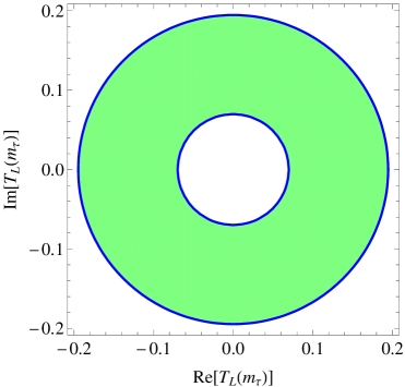
Figure 4: The allowed regions for the real and imaginary components of the leptoquark running couplings $S_{L}(m_{\tau})$ and $T_{L}(m_{\tau})$ with $S_{L}(m_{LQ})=\pm 4\;T_{L}(m_{LQ})$ at $m_{\rm LQ}=1000$ GeV. The constraint on $S_{L}(m_{\tau})$ is from $\tau^{-}\rightarrow\pi^{-}\nu_{\tau}$ and $T_{L}(m_{\tau})$ is from $\tau^{-}\rightarrow\pi^{-}\pi^{0}\nu_{\tau}$.

In the $V\pm A$ case, the couplings can be constrained by both $\tau^{-}\rightarrow\nu_{\tau}+\pi^{-}$ and $\tau\to\pi^{-}+\pi^{0}+\nu_{\tau}$ decays. Considering the first process the branching ratio is given as

$$Br^{\pi}_{V\pm A} = Br^{\pi}_{\rm SM}(1+r^{\pi}_{V\pm A})^{2}\,,$$ (48)

where the $V\pm A$ contribution is

$$r^{\pi}_{V\pm A} = V_{L}-V_{R}\,.$$ (49)

From the second process, the branching ratio is given as

$$Br^{\pi\pi}_{V\pm A} = Br^{\pi\pi}_{\rm SM}(1+r^{\pi\pi}_{V\pm A})^{2}\,,$$ (50)

where the $V\pm A$ contribution is

$$r^{\pi\pi}_{V\pm A} = V_{L}+V_{R}\,.$$ (51)

If we take the couplings to be real, the contour plot in Fig. 5 shows the allowed region. The allowed regions for the real and imaginary parts, if the couplings are taken to be complex, are shown in the contour plot in Fig. 6.

Note, even though we consider complex couplings in the constraint equations in this section, we take the couplings to be real for the scattering calculations.

Figure 5: The allowed region (green area) for the left- and right-handed couplings $V_{L}$ and $V_{R}$. The constraints are from $\tau^{-}\rightarrow\pi^{-}\nu_{\tau}$ and $\tau^{-}\rightarrow\pi^{-}\pi^{0}\nu_{\tau}$.

Figure 6: The allowed regions for the left- and right-handed complex couplings $V_{L}$ and $V_{R}$. The constraint are from $\tau^{-}\rightarrow\pi^{-}\nu_{\tau}$ and $\tau^{-}\rightarrow\pi^{-}\pi^{0}\nu_{\tau}$. Left panel: we take $V_{R}=0$ and treat $V_{L}$ as a complex coupling. The allowed region is the contour ring. Right panel: we take $V_{L}=0$ and treat $V_{R}$ as a complex coupling. The allowed region is the overlap area between the two contour rings.

4 Numerical analysis

In this section the sensitivity of the neutrino cross-section scattering to the scalar and tensor interactions, explicit Leptoquark model, and $V\pm A$ interactions is discussed. We study the ratio of the total cross section, $d\sigma/dxdy$, and $d\sigma/dt$ for the tau-neutrino to the muon-neutrino scattering. We also show the results of the total cross section, $d\sigma/dxdy$, and $d\sigma/dt$ for the process $\nu_{\tau}+N\to\tau+X$.

4.1 Scalar and Tensor Interactions

The ratio of the total cross section is shown in Fig. 7 while the ratio of the differential cross sections $d\sigma/dxdy$ and $d\sigma/dt$ are given in Figs. (8, 9). The impact of the new physics is clearly detectable in the ratio of the total cross section and the differential cross sections. The new physics effect is also observable in the total cross section, $d\sigma/dxdy$, and $d\sigma/dt$ for the process $\nu_{\tau}+N\to\tau+X$, as shown in Figs. (10, 11, 12).

4.2 Explicit Leptoquark Model

Here we take $m_{\rm LQ}=1$ TeV. In Figs. (13, 14, 15), we show the differential cross section $d\sigma/dt$, its ratio, and the total cross section for the particular models $S_{L}(m_{\rm LQ})=\pm 4\;T_{L}(m_{\rm LQ})$. The impact of the new physics is clearly detectable.

4.3 $V\pm A$ Interactions

The ratio of the total cross section, $d\sigma/dxdy$, $d\sigma/dt$ are shown in Figs. (16, 17, 18), respectively. The figures show that the effect of $V\pm A$ new physics is small in the neutrino cross section. The new physics effect is small in the total cross section, $d\sigma/dxdy$, and $d\sigma/dt$ for the process $\nu_{\tau}+N\to\tau+X$, as shown in Figs. (19, 20, 21).

Figure 7: $S\pm T$ model: The ratio between the total cross section of $\nu_{\tau}+N\to\tau+X$ to $\nu_{\mu}+N\to\mu+X$ with Scalar-Tensor couplings. The green solid line corresponds to the standard model predictions $S_{R}=S_{L}=T_{L}=0$. The blue dashed, red dotdashed and black dotted lines correspond to $(S_{R},S_{L},T_{L})=(-0.19,0.68,0.072),\;(1.98,0.42,-0.13),\;(-1.87,-1.31,0.18)$.

Figure 8: $S\pm T$ model: The ratio between the differential cross section $(d\sigma/dxdy)$ of $\nu_{\tau}+N\to\tau+X$ to $\nu_{\mu}+N\to\mu+X$ with Scalar-Tensor couplings. The green lines correspond to the standard model predictions $S_{R}=S_{L}=T_{L}=0$. The blue, black, and red lines correspond to $(S_{R},S_{L},T_{L})=(-0.19,0.68,0.072),\;(1.98,0.42,-0.13),\;(-1.87,-1.31,0.18)$. The blue and green dashed lines correspond to $(x,y)=(0.95,A+B)$. The black and green dotdashed lines correspond to $(x,y)=(0.475,(A+B)/2)$. The red and green dotted lines correspond to $(x,y)=(\frac{m_{\tau}^{2}}{2M(E_{\nu}-m_{\tau})},A-B)$.

Figure 9: $S\pm T$ model: The ratio between the differential cross section $(d\sigma/dt)$ of $\nu_{\tau}+N\to\tau+X$ to $\nu_{\mu}+N\to\mu+X$ in the Scalar-Tensor model. The green dashed, dotted and dotdashed lines correspond to the standard model predictions $S_{R}=S_{L}=T_{L}=0$ at $E_{\nu}=30,20,10$ GeV, respectively. The blue dashed, black dotted, and red dotdashed lines correspond to $(S_{R},S_{L},T_{L})=(-0.19,0.68,0.072),\;(1.98,0.42,-0.13),\;(-1.87,-1.31,0.18)$ at $E_{\nu}=30,20,10$ GeV, respectively. The physical regions of the momentum transfer is taken to be $Q^{2}_{-}(W_{cut})\leq Q^{2}\leq Q^{2}_{+}(W_{cut})$.

Figure 10: $S\pm T$ model: The total cross section of $\nu_{\tau}+N\to\tau+X$ in the Scalar-Tensor model. The green solid line corresponds to the standard model predictions $S_{R}=S_{L}=T_{L}=0$. The blue dashed, black dotted and red dotdashed lines correspond to $(S_{R},S_{L},T_{L})=(-0.19,0.68,0.072),\;(1.98,0.42,-0.13),\;(-1.87,-1.31,0.18)$.

Figure 11: $S\pm T$ model: The differential cross section $(d\sigma/dxdy)$ of $\nu_{\tau}+N\to\tau+X$ in the Scalar-Tensor model. The green lines correspond to the standard model predictions $S_{R}=S_{L}=T_{L}=0$. The blue, black, and red lines correspond to $(S_{R},S_{L},T_{L})=(-0.19,0.68,0.072),\;(1.98,0.42,-0.13),\;(-1.87,-1.31,0.18)$. The blue and green dashed lines correspond to $(x,y)=(0.95,A+B)$. The black and green dotdashed lines correspond to $(x,y)=(0.475,(A+B)/2)$. The red and green dotted lines correspond to $(x,y)=(\frac{m_{\tau}^{2}}{2M(E_{\nu}-m_{\tau})},A-B)$.

Figure 12: $S\pm T$ model: The differential cross section $(d\sigma/dt)$ of $\nu_{\tau}+N\to\tau+X$ in the Scalar-Tensor model. The green dashed, dotted and dotdashed lines correspond to the standard model predictions $S_{R}=S_{L}=T_{L}=0$ at $E_{\nu}=30$(left), $20$(middle) and $10$(right) GeV, respectively. The blue dashed, black dotted, and red dotdashed lines correspond to $(S_{R},S_{L},T_{L})=(-1.87,-1.31,0.18)$ at $E_{\nu}=30$(left), $20$(middle) and $10$(right) GeV, respectively. The physical regions of the momentum transfer is taken to be $Q^{2}_{-}(W_{cut})\leq Q^{2}\leq Q^{2}_{+}(W_{cut})$.

Figure 13: Leptoquark: The ratio between the differential cross section $(d\sigma/dt)$ of $\nu_{\tau}+N\to\tau+X$ to $\nu_{\mu}+N\to\mu+X$ in the Leptoquark model with $S_{L}(m_{\rm LQ})=\pm 4\;T_{L}(m_{\rm LQ})$ at $m_{\rm LQ}=1000$ GeV. The green dashed, dotted and dotdashed lines correspond to the standard model predictions $S_{R}=S_{L}=T_{L}=0$ at $E_{\nu}=30,20,10$ GeV, respectively. The blue, black, and red lines correspond to $(Re[S_{L}(m_{LQ})],Im[S_{L}(m_{LQ})],Re[T_{L}(m_{LQ})],Im[T_{L}(m_{LQ})])=(0.56,0.60,0.14,0.15)$ at $E_{\nu}=30,20,10$ GeV, respectively. The physical regions of the momentum transfer is taken to be $Q^{2}_{-}(W_{cut})\leq Q^{2}\leq Q^{2}_{+}(W_{cut})$.

Figure 14: Leptoquark: The differential cross section $(d\sigma/dt)$ of $\nu_{\tau}+N\to\tau+X$ in the Leptoquark model with $S_{L}(m_{\rm LQ})=\pm 4\;T_{L}(m_{\rm LQ})$ at $m_{\rm LQ}=1000$ GeV. The green dashed, dotted and dotdashed lines correspond to the standard model predictions $S_{R}=S_{L}=T_{L}=0$ at $E_{\nu}=$ 30(left), 20(middle) and 10(right) GeV, respectively. The blue, black, and red lines correspond to $(Re[S_{L}(m_{LQ})],Im[S_{L}(m_{LQ})],Re[T_{L}(m_{LQ})],Im[T_{L}(m_{LQ})])=(0.56,0.60,0.14,0.15)$ at $E_{\nu}=$ 30(left), 20(middle) and 10(right) GeV, respectively. The physical regions of the momentum transfer is taken to be $Q^{2}_{-}(W_{cut})\leq Q^{2}\leq Q^{2}_{+}(W_{cut})$.

Figure 15: Leptoquark: The total cross section in the Leptoquark model with $S_{L}(m_{\rm LQ})=\pm 4\;T_{L}(m_{\rm LQ})$ at $m_{\rm LQ}=1000$ GeV. The green line corresponds to the standard model predictions $S_{R}=S_{L}=T_{L}=0$. The blue line corresponds to $(Re[S_{L}(m_{LQ})],Im[S_{L}(m_{LQ})],Re[T_{L}(m_{LQ})],Im[T_{L}(m_{LQ})])=(0.56,0.60,0.14,0.15)$. The physical regions of the momentum transfer is taken to be $Q^{2}_{-}(W_{cut})\leq Q^{2}\leq Q^{2}_{+}(W_{cut})$.

Figure 16: $V\pm A$ model: The ratio between the total cross section of $\nu_{\tau}+N\to\tau+X$ to $\nu_{\mu}+N\to\mu+X$ in the $V\pm A$ model. The green line corresponds to the standard model predictions $V_{L}=V_{R}=0$. The red dotdashed line corresponds to $(V_{L},V_{R})=(0.016,0.006)$.

Figure 17: $V\pm A$ model: The ratio between the differential cross section $(d\sigma/dxdy)$ of $\nu_{\tau}+N\to\tau+X$ to $\nu_{\mu}+N\to\mu+X$ in the $V\pm A$ model. The green lines correspond to the standard model predictions $V_{L}=V_{R}=0$. The blue, black, and red lines correspond to $(V_{L},V_{R})=(0.016,0.006)$. The blue and green dashed lines correspond to $(x,y)=(0.95,A+B)$. The red and green dotdashed lines correspond to $(x,y)=(0.475,(A+B)/2)$. The black and green dotted lines correspond $(x,y)=(\frac{m_{\tau}^{2}}{2M(E_{\nu}-m_{\tau})},A-B)$.

Figure 18: $V\pm A$ model: The ratio between the differential cross section $(d\sigma/dt)$ of $\nu_{\tau}+N\to\tau+X$ to $\nu_{\mu}+N\to\mu+X$ in the $V\pm A$ model. The green lines correspond to the standard model predictions $V_{L}=V_{R}=0$. The blue, black, and red lines correspond to $(V_{L},V_{R})=(0.016,0.006)$ at $E_{\nu}=30,20,10$ GeV, respectively. The physical regions of the momentum transfer is taken to be $Q^{2}_{-}(W_{cut})\leq Q^{2}\leq Q^{2}_{+}(W_{cut})$.

Figure 19: $V\pm A$ model: The total cross section of $\nu_{\tau}+N\to\tau+X$ in the $V\pm A$ model. The green line corresponds to the standard model predictions $V_{L}=V_{R}=0$. The red dotdashed line corresponds to $(V_{L},V_{R})=(0.016,0.006)$.

Figure 20: $V\pm A$ model: The differential cross section $(d\sigma/dxdy)$ of $\nu_{\tau}+N\to\tau+X$ in the $V\pm A$ model. The green lines correspond to the standard model predictions $V_{L}=V_{R}=0$. The blue, black, and red lines correspond to $(V_{L},V_{R})=(0.016,0.006)$. The blue and green dashed lines correspond to $(x,y)=(0.95,A+B)$. The red and green dotdashed lines correspond to $(x,y)=(0.475,(A+B)/2)$. The black and green dotted lines correspond to $(x,y)=(\frac{m_{\tau}^{2}}{2M(E_{\nu}-m_{\tau})},A-B)$.

Figure 21: $V\pm A$ model: The differential cross section $(d\sigma/dt)$ of $\nu_{\tau}+N\to\tau+X$ in the $V\pm A$ model. The green lines correspond to the standard model predictions $V_{L}=V_{R}=0$. The blue, black, and red lines correspond to $(V_{L},V_{R})=(0.016,0.006)$ at $E_{\nu}=30,20,10$ GeV, respectively. The physical regions of the momentum transfer is taken to be $Q^{2}_{-}(W_{cut})\leq Q^{2}\leq Q^{2}_{+}(W_{cut})$

5 Conclusion

In this paper we discussed tests of lepton non-universal interactions through $\nu_{\tau}$ scattering. We adopted an effective Lagrangian description of new physics and considered explicit leptoquark models for our calculations. The parameters of the new physics were constrained by single pion and two pion $\tau$ decays, $\tau^{-}(k_{1})\rightarrow\nu_{\tau}(k_{2})+\pi^{-}(q)$ and $\tau(p)\to\pi^{-}(p_{1})+\pi^{0}(p_{2})+\nu_{\tau}(p_{3})$ , which are well measured. We then discussed the ratio of the total and differential cross sections for the two deep inelastic scattering processes $\nu_{\tau}+N\to\tau+X$ and $\nu_{\mu}+N\to\mu+X$ as a probe of the new physics in the neutrino cross-section experiments. In the ratio of cross sections, the uncertainty of the parton distribution functions is expected to cancel out leading to precise results. In the effective Lagrangian framework we looked at models with scalar and tensor interactions. As an explicit realization of such models we considered leptoquark models where scalar and tensor couplings arise with relations between the couplings. Our results showed significant new physics effects, both in the total cross sections as well as in the differential distributions for $\nu_{\tau}+N\to\tau+X$, are allowed with the present constraints. These new physics effects could be observed at future proposed $\nu_{\tau}$ scattering experiments. We also considered vector-axial vector new physics operators in our analysis. The results showed that the new physics effect is small in this case.

Appendix (A)

Here, we give details of the calculations of the process $\tau(p)\to\nu_{\tau}(p_{3})+\pi^{-}(p_{1})+\pi^{0}(p_{2})$. In the rest frame of $\pi^{-}$ and $\pi^{0}$,

$$p=\begin{pmatrix}E,&\vec{P}\\ \end{pmatrix},p_{1}=\begin{pmatrix}E_{1},&\vec{P_{1}}\\ \end{pmatrix},p_{2}=\begin{pmatrix}E_{2},&-\vec{P_{1}}\\ \end{pmatrix},p_{3}=\begin{pmatrix}E_{3},&\vec{P}\\ \end{pmatrix},$$ (52)

$$k=p_{1}-p_{2}=\begin{pmatrix}E_{1}-E_{2},&2\vec{P_{1}}\\ \end{pmatrix},q=p_{1}+p_{2}=\begin{pmatrix}E_{1}+E_{2},&0\\ \end{pmatrix},$$ (53)

and we define two variables,

$$m_{12}^{2} = (p_{1}+p_{2})^{2}=q^{2},$$

$$m_{23}^{2} = (p_{2}+p_{3})^{2}.$$ (54)

Then,

$$d\Gamma=\frac{1}{(2\pi)^{3}}\frac{1}{32m_{\tau}^{3}}Xdm_{12}^{2}dm_{23}^{2},$$ (55)

with

$$X=\frac{1}{2}\sum_{spin}|M_{SM}+M_{T}|^{2}=\frac{1}{2}\sum_{spin}|M_{SM}|^{2}+\frac{1}{2}\sum_{spin}|M_{T}|^{2},$$ (56)

where $M_{SM}$ and $M_{T}$ are given in Eqs. (43, 44), and the cross terms are zero.

By averaging the spin, we get

$$X_{SM}=4G_{F}^{2}V_{ud}^{2}F^{2}(Q^{2})[2(k\cdot p)(k\cdot p_{3})-k^{2}(p\cdot p_{3})],$$ (57)

and,

$$X_{T} = 16G_{F}^{2}V_{ud}^{2}T_{L}^{2}\frac{F^{2}(Q^{2})}{q^{2}}[(k\cdot q)^{2}(-p\cdot p_{3})+2(k\cdot q)((k\cdot p_{3})(p\cdot q)$$

$$+(k\cdot p)(p_{3}\cdot q))-2q^{2}(k\cdot p)(k\cdot p_{3})+k^{2}(q^{2}(p\cdot p_{3})-2(p\cdot q)(p_{3}\cdot q))].$$

All these $X^{\prime}s$ can be expressed in terms of $m_{12}^{2}$ and $m_{23}^{2}$ because

$$E_{1}=\frac{m_{12}^{2}-m_{2}^{2}+m_{1}^{2}}{2m_{12}},$$ (59)

$$E_{2}=\frac{m_{12}^{2}-m_{1}^{2}+m_{2}^{2}}{2m_{12}},$$ (60)

$$E_{3}=\frac{M^{2}-m_{12}^{2}-m_{3}^{2}}{2m_{12}},$$ (61)

$$E=\frac{M^{2}+m_{12}^{2}-m_{3}^{2}}{2m_{12}},$$ (62)

$$2\vec{p_{1}}\cdot\vec{p}=m_{23}^{2}-m_{2}^{2}-m_{3}^{2}-2E_{2}E_{3},$$ (63)

$$|\vec{p}|=\sqrt{E^{2}-M^{2}},$$ (64)

$$|\vec{p_{1}}|=\sqrt{E_{1}^{2}-m_{1}^{2}},$$ (65)

with $M=m_{\tau}=1.77$ GeV, $m_{1}=m_{\pi^{-}}=0.140$ GeV, $m_{2}=m_{\pi^{0}}=0.135$ GeV, $m_{3}=m_{\nu_{\tau}}=0$.

Let’s work on the SM case first and set

$$A_{1} =k\cdot p=E(E_{1}-E_{2})-2\vec{p_{1}}\cdot\vec{p}$$

$$=E(E_{1}-E_{2})+2E_{2}E_{3}+m_{2}^{2}+m_{3}^{2}-m_{23}^{2},$$ (66)

$$A_{2} =k\cdot p_{3}=E_{3}(E_{1}-E_{2})-2\vec{p_{1}}\cdot\vec{p}$$

$$=E_{3}(E_{1}-E_{2})+2E_{2}E_{3}+m_{2}^{2}+m_{3}^{2}-m_{23}^{2},$$ (67)

$$A_{3} =k^{2}=(E_{1}-E_{2})^{2}-4\vec{p_{1}}^{2}$$

$$=(E_{1}-E_{2})^{2}-4(E_{1}^{2}-m_{1}^{2}),$$ (68)

$$A_{4} =p\cdot p_{3}=E_{1}E_{3}-\vec{p}^{2}$$

$$=E_{1}E_{3}-E^{2}+M^{2}.$$ (69)

Then,

$$X_{SM}=4G_{F}^{2}V_{ud}^{2}F^{2}(Q^{2})[2A_{1}A_{2}-A_{3}A_{4}].$$ (70)

Now, let us integrate $X_{SM}$ by $m_{23}^{2}$ within the limits

$$(m_{23}^{2})_{max}=(E_{2}+E_{3})^{2}-\left(\sqrt{E_{2}^{2}-m_{2}^{2}}-\sqrt{E_{3}^{2}-m_{3}^{2}}\right)^{2},$$ (71)

$$(m_{23}^{2})_{min}=(E_{2}+E_{3})^{2}-\left(\sqrt{E_{2}^{2}-m_{2}^{2}}+\sqrt{E_{3}^{2}-m_{3}^{2}}\right)^{2},$$ (72)

where $m_{1}=m_{2}=m_{\pi}$, $m^{2}_{12}=Q^{2}$ and $M=m_{\tau}$. One gets

$$\Gamma_{SM}=\frac{4G^{2}_{F}m^{5}_{\tau}}{96(2\pi)^{3}}\frac{cos\theta_{c}}{2}\int_{Q^{2}_{min}}^{Q^{2}_{max}}\frac{dQ^{2}}{m^{2}_{\tau}}F^{2}(Q^{2})\left(1-\frac{Q^{2}}{m^{2}_{\tau}}\right)^{2}\left(1+2\frac{Q^{2}}{m^{2}_{\tau}}\right)\left(1-\frac{4m^{2}_{\pi}}{Q^{2}}\right)^{3/2}.$$ (73)

Now, we can integrate over $m_{12}^{2}$ within the limits

$$Q^{2}_{max} = (m_{12}^{2})_{max}=(M-m_{1})^{2},$$

$$Q^{2}_{min} = (m_{12}^{2})_{min}=(m_{1}+m_{2})^{2}.$$ (74)

Now let’s work on the tensor leptoquark case, we set

$$B_{1} =k\cdot q=E^{2}_{1}-E^{2}_{2},$$ (75)

$$B_{2} =p\cdot p_{3}=EE_{3}-\vec{p}^{2},$$ (76)

$$B_{3} =k\cdot p_{3}=E_{3}(E_{1}-E_{2})-2\vec{p}\cdot\vec{p_{1}},$$ (77)

$$B_{4} =p\cdot q=E(E_{1}+E^{2}),$$ (78)

$$B_{5} =k\cdot p_{3}=E(E_{1}-E_{2})-2\vec{p}\cdot\vec{p_{1}},$$ (79)

$$B_{6} =P_{3}\cdot q=E_{3}(E_{1}+E_{2}),$$ (80)

$$B_{7} =q^{2}=(E_{1}+E_{2})^{2},$$ (81)

$$B_{8} =k^{2}=(E_{1}-E_{2})^{2}-4\vec{p_{1}}^{2}.$$ (82)

Then,

$$X_{T}=8G_{F}^{2}V_{ud}^{2}T_{L}^{2}F_{T}^{2}(q^{2})\left[-B_{1}^{2}B_{3}+2B_{1}(B_{3}B_{4}+B_{1}B_{6})-2B_{7}B_{1}B_{5}+B_{8}(B_{7}B_{2}-2B_{4}B_{6})\right].$$ (83)

Numerically, we can get $\Gamma_{T}=3.43\times 10^{-12}T_{L}^{2}$ GeV.

Appendix (B)

In the decay process $\tau^{-}\rightarrow\nu_{\tau}+\pi^{-}$, the SM hadronic current is given in Eq. 34. By multiplying the current by $q^{\mu}=p^{\mu}_{d}+p^{\mu}_{u}$, one can find the NP scalar current given by

$$\langle 0|\bar{d}(A_{S}-B_{S}\gamma^{5})u|\pi(q)\rangle=\frac{i\sqrt{2}f_{\pi}m_{\pi}^{2}}{m_{u}+m_{d}}B_{S}.$$ (84)

If one multiplies the SM current by $k^{\mu}=p^{\mu}_{d}-p^{\mu}_{u}$, the scalar current will be

$$\langle 0|\bar{d}(A_{S}-B_{S}\gamma^{5})u|\pi(q)\rangle=i\sqrt{2}f_{\pi}(m_{u}+m_{d})B_{S}.$$ (85)

Now, by multiplying the two equations above and taking the square root, we end up with scalar current that is independent of the quark masses

$$\langle 0|\bar{d}(A_{S}-B_{S}\gamma^{5})u|\pi(q)\rangle=i\sqrt{2}f_{\pi}m_{\pi}B_{S}.$$ (86)

In the process $\tau^{-}(p)\to\pi^{-}(p_{1})+\pi^{0}(p_{2})+\nu_{\tau}(p_{3})$, the NP tensor current is given in Eq. 46. Here $p_{1}^{\mu}=p^{\mu}_{d}+p^{\mu}_{q}$ and $p_{2}^{\mu}=p^{\mu}_{u}-p^{\mu}_{q}$, where $p_{u}$ and $p_{d}$ are the momenta of the up and down quarks that come from the tau decay, and $(p_{q},-p_{q})$ are the momenta of the quark-antiquark pair from the vacuum that pair up with the up and down quarks to form $\pi^{0}$ and $\pi^{-}$. By multiplying the current by $q^{\mu}=p^{\mu}_{1}+p^{\mu}_{2}=p^{\mu}_{d}-p^{\mu}_{u}$ and using the equation of motion, in the isospin symmetry limit, one gets the form factor

$$F_{T}=-i\frac{(m_{u}+m_{d})}{q^{2}}F.$$ (87)

If one multiplies the tensor current by $k^{\mu}=p^{\mu}_{1}-p^{\mu}_{2}=p^{\mu}_{d}-p^{\mu}_{u}+2p^{\mu}_{q}$, the form factor will be given by

$$F_{T}=\frac{-iF}{(m_{d}+m_{u})-\left(1-2\frac{p_{q}\cdot k}{k^{2}}\right)\left(\frac{m_{\pi^{-}}^{2}-m_{\pi^{0}}^{2}}{m_{d}-m_{u}}\right)}.$$ (88)

Now if the $\pi\pi$ is dominantly coming from a vector resonance then we can expect that the distribution of the momenta of the quarks inside the resonance will be peaked around $p_{u}=p_{d}$. In this limit the second term in the denominator above vanishes as $\left(1-2\frac{p_{q}\cdot k}{k^{2}}\right)=0$ . Hence,by taking the second term in the denominator small, we get

$$F_{T}=-i\frac{1}{(m_{u}+m_{d})}F.$$ (89)

Now, by multiplying the two equations above and taking the square root, the form factor will be independent of the quark masses

$$F_{T}=\frac{-iF}{\sqrt{q^{2}}}.$$ (90)

References

- [1] J. P. Lees et al. [BaBar Collaboration], Phys. Rev. Lett. 109, 101802 (2012) [arXiv:1205.5442 [hep-ex]].
- [2] J. P. Lees et al. [BaBar Collaboration], Phys. Rev. D 88, 072012 (2013) [arXiv:1303.0571 [hep-ex]].
- [3] S. Fajfer, J. F. Kamenik and I. Nisandzic, [arXiv:1203.2654 [hep-ph]]; Y. Sakaki and H. Tanaka, [arXiv:1205.4908 [hep-ph]].
- [4] See for instance, A. Datta, M. Duraisamy and D. Ghosh, Phys. Rev. D 86, 034027 (2012) [arXiv:1206.3760 [hep-ph]]; M. Duraisamy and A. Datta, JHEP 1309, 059 (2013) [arXiv:1302.7031 [hep-ph]]; M. Duraisamy, P. Sharma and A. Datta, Phys. Rev. D 90, 074013 (2014) [arXiv:1405.3719 [hep-ph]]; S. Shivashankara, W. Wu and A. Datta, arXiv:1502.07230 [hep-ph].
- [5] B. Bhattacharya, A. Datta, D. London and S. Shivashankara, Phys. Lett. B 742, 370 (2015) [arXiv:1412.7164 [hep-ph]].
- [6] R. Aaij et al. [LHCb Collaboration], Phys. Rev. Lett. 113, 151601 (2014) [arXiv:1406.6482 [hep-ex]].
- [7] G. Hiller and F. Kruger, Phys. Rev. D 69, 074020 (2004) [arXiv:hep-ph/0310219]; C. Bobeth, G. Hiller and G. Piranishvili, JHEP 0712, 040 (2007) [arXiv:0709.4174 [hep-ph]]; C. Bouchard et al. [HPQCD Collaboration], Phys. Rev. Lett. 111, no. 16, 162002 (2013) [Erratum-ibid. 112, no. 14, 149902 (2014)] [arXiv:1306.0434 [hep-ph]].
- [8] See for example A. K. Alok, A. Dighe, D. Ghosh, D. London, J. Matias, M. Nagashima and A. Szynkman, JHEP 1002, 053 (2010) [arXiv:0912.1382 [hep-ph]]; A. K. Alok, A. Datta, A. Dighe, M. Duraisamy, D. Ghosh and D. London, JHEP 1111, 121 (2011) [arXiv:1008.2367 [hep-ph]], JHEP 1111, 122 (2011) [arXiv:1103.5344 [hep-ph]];
- [9] R. Aaij et al. [LHCb Collaboration], Phys. Rev. Lett. 111 (2013) 191801 [arXiv:1308.1707 [hep-ex]].
- [10] See for example: A. Datta, M. Duraisamy and D. Ghosh, Phys. Rev. D 89 (2014) 071501 [arXiv:1310.1937 [hep-ph]];
- [11] K. Kodama et al. [DONuT Collaboration], Phys. Rev. D 78, 052002 (2008) [arXiv:0711.0728 [hep-ex]].
- [12] A. Rashed, P. Sharma and A. Datta, Nucl. Phys. B 877, 662 (2013) [arXiv:1303.4332 [hep-ph]]; A. Rashed, M. Duraisamy and A. Datta, Phys. Rev. D 87, no. 1, 013002 (2013) [arXiv:1204.2023 [hep-ph]].
- [13] E. Graverini, N. Serra and B. Storaci, arXiv:1503.08624 [hep-ex]; D. Gorbunov, A. Makarov and I. Timiryasov, Phys. Rev. D 91, no. 3, 035027 (2015) [arXiv:1411.4007 [hep-ph]].
- [14] T. Bhattacharya, V. Cirigliano, S. D. Cohen, A. Filipuzzi, M. Gonzalez-Alonso, M. L. Graesser, R. Gupta and H. -W. Lin, Phys. Rev. D 85, 054512 (2012) [arXiv:1110.6448 [hep-ph]]; C. -H. Chen and C. -Q. Geng, Phys. Rev. D 71, 077501 (2005) [hep-ph/0503123].
- [15] A. Datta, P. J. O’Donnell, Z. H. Lin, X. Zhang and T. Huang, Phys. Lett. B 483, 203 (2000) [hep-ph/0001059].
- [16] S. Kretzer and M. H. Reno, Phys. Rev. D66(2002)113007.
- [17] C. H. Albright and C. Jarlskog, Nucl. Phys. B84(1975)467.
- [18] W. Buchmuller, R. Ruckl and D. Wyler, Phys. Lett. B 191, 442 (1987) [Erratum-ibid. B 448, 320 (1999)].
- [19] F. S. Queiroz, K. Sinha and A. Strumia, Phys. Rev. D 91, no. 3, 035006 (2015) [arXiv:1409.6301 [hep-ph]].
- [20] W. Buchmuller, R. Ruckl and D. Wyler, Phys.Lett. B 191 (1987) 442.
- [21] I. Dorsner, S. Fajfer, N. Kosnik and I. Nisandzic, JHEP 1311, 084 (2013) [arXiv:1306.6493 [hep-ph]].
- [22] K. Hagiwara, K. Mawatari and H. Yokoya, Nucl. Phys. B 668, 364 (2003) [Erratum-ibid. B 701, 405 (2004)] [hep-ph/0305324].
- [23] K. G. Chetyrkin, Phys. Lett. B 404, 161 (1997) [hep-ph/9703278].
- [24] J. A. Gracey, Phys. Lett. B 488, 175 (2000) [hep-ph/0007171].
- [25] K. Nakamura et al. (Particle Data Group), J. Phys. G 37, 075021 (2010) and 2011 partial update for the 2012 edition.
- [26] M. Davier, A. Hocker and Z. Zhang, Rev. Mod. Phys. 78, 1043 (2006) [hep-ph/0507078].
- [27] B. C. Barish, In *Stanford 1989, Proceedings, Study of tau, charm and J/psi physics* 113-126 and Caltech Pasadena - CALT-68-1580 (89,rec.Oct.) 14 p
- [28] J. H. Kuhn, A. Santamaria, Zeitschrift fur Physik C - Particles and Fields 1990, Volume 48, Issue 3, pp 445-452
- [29] A. Bernicha, G. Lopez Castro and J. Pestieau, Phys. Rev. D 53, 4089 (1996) [hep-ph/9510435].
- [30] K.A. Olive et al. (Particle Data Group), Chin. Phys. C, 38, 090001 (2014).