The VISTA Orion mini-survey:
star formation in the Lynds 1630 North cloud

The Orion cloud complex presents a variety of star formation mechanisms and properties and it is still one of the most intriguing targets for star formation studies. We present VISTA/VIRCAM near-infrared observations of the L1630N star forming region, including the stellar clusters NGC 2068 and NGC 2071, in the Orion molecular cloud B and discuss them in combination with Spitzer data. We select 186 young stellar object (YSO) candidates in the region on the basis of multi-colour criteria, confirm the YSO nature of the majority of them using published spectroscopy from the literature, and use this sample to investigate the overall star formation properties in L1630N. The K-band luminosity function of L1630N is remarkably similar to that of the Trapezium cluster, i.e., it presents a broad peak in the range 0.3-0.7 M_⊙ and a fraction of sub-stellar objects of $\sim$20%. The fraction of YSOs still surrounded by disk/envelopes is very high ($\sim$85%) compared to other star forming regions of similar age (1-2 Myr), but includes some uncertain corrections for diskless YSOs. Yet, a possibly high disk fraction together with the fact that 1/3 of the cloud mass has a gas surface density above the threshold for star formation ($\sim$129 M_⊙ pc^-2), points towards a still on-going star formation activity in L1630N. The star formation efficiency (SFE), star formation rate (SFR) and density of star formation of L1630N are within the ranges estimated for galactic star forming regions by the Spitzer ”core to disk” and ”Gould’s Belt” surveys. However, the SFE and SFR are lower than the average value measured in the Orion A cloud and, in particular, lower than that in the southern regions of L1630. This might suggest different star formation mechanisms within the L1630 cloud complex.

1 Introduction

Observations of young stellar populations in nearby star forming regions are important tools to understand the interplay between the outcome of the star formation process and the original environment from which the stellar ensembles emerged. While details of the star formation process and its physics are often tested with targeted investigations on small spatial scales, global properties are best assessed with wide-field imaging surveys in the infrared thereby accomplishing large-scale studies in a homogenous way.

The Spitzer c2d (Evans et al., 2009) and Spitzer Gould Belt (GB) Legacy surveys (e.g., Spezzi et al., 2011; Hatchell et al., 2012; Dunham et al., 2013) effectively traced the population of young stellar objects (YSOs) in several nearby star forming regions. These studies have shown that current star-formation efficiencies are in the range from 3% to 6%, and that star formation is highly concentrated to regions of high extinction with the youngest objects being strongly associated with dense cores. The great majority (90%) of the young stars lie within loose clusters with at least 35 members and a stellar density of 1 M${}_{\odot}\,$pc^-3 (Evans et al., 2009, and references therein). The c2d and GB surveys have also shown that the star-formation surface density in galactic star forming regions is more than an order of magnitude larger than predicted from extragalactic star formation rate $-$ gas relationships, e.g. the Kennicutt-Schmidt law (Evans et al., 2009; Heiderman et al., 2010).

Among the most-studied nearby active star formation sites are the Orion A and Orion B molecular clouds. The clouds have similar masses of a few $10^{4}$ M_☉ and appear physically connected, indicating that they stem from the same overall giant molecular cloud complex. However, star formation differs quite significantly between the clouds. In Orion B almost all stars ($\sim$90%) formed in stellar clusters (Lada et al. 1991), which concentrate at two major sites, one in the southern part of the Orion B cloud where the clusters NGC2024/23 are located and one in the northern part of Orion B (also named L1630N) with the clusters NGC2068/71. Orion A, on the other hand, shows a substantial population of distributed star formation with $\sim 70$% of the stars forming in isolation (Strom et al. 1993, Fang et al. 2009), with the exception of the Orion Nebula Cluster which lies at the northernmost end of Orion A. Orion B contains several early B-type stars and at least one O star, while Orion A (excluding the ONC) possibly has no stars earlier than B4 and is apparently deficient in early type massive stars when compared to its known numbers of low-mass stars (Hsu et al., 2012). Furthermore, large-scale molecular gas maps indicate clear substructure on scales $<$2 pc in Orion A, whereas Orion B displays very little substructure, although highly filamentary molecular gas seems associated with the star forming regions in the northern part of Orion B, i.e. in L1630 N (Gibb, 2008, and references therein).

In this paper we present multi-band wide-field near-infrared observations obtained with VISTA/VIRCAM, combined with mid-infrared data from Spitzer, covering approximately 1.6 square degrees in the northern part of the Orion molecular cloud B, i.e. in L1630 N

The L1630 N region contains the prominent bright optical reflection nebulosities NGC 2068 and NGC 2071 which, observed at near-infrared wavelengths, reveal their full nature as young stellar clusters. Flaherty & Muzerolle (2008) determined the clusters’ age as 1-2 Myr, depending on the models used, and confirmed 67 stellar members through optical spectroscopy. However, the use of optical spectroscopy, combined with 2MASS photometry, limited their study to the least embedded and slightly higher mass objects. Fang et al. (2009) performed also optical spectroscopy of 132 stars in the region. This latter sample includes all the stars previously caracterized by Flaherty & Muzerolle (2008) and several additional objects classified as Pre-Main Sequence (PMS) stars by Fang et al. (2009). These authors find a much higher disk frequency in L1630 N in comparison with L1641 (Orion A) and with other star forming regions of similar age like Chamaeleon I and IC 348, but they also caution that the results are upper limits as their sample is biased against non-disk bearing young stars. A recent study by Hsu et al. (2012) employed a photometric and spectroscopic survey to enlarge the population of confirmed members in L1641 and find the disk frequency similarly high as for L1630. Clearly, the physical characterisation of young star properties gets better defined as our census of the young star populations becomes complete.

The combination of wide field coverage and excellent sensitivity of our survey enables us to uncover a large young stellar object (YSO) population in L1630 N, which increases the number of previously known YSOs by a factor 1.5, and thereby allows us to analyse the global star formation properties in this region.

After the description of the VISTA-Orion catalog and the extraction of the data for this work in Sect. 2, we present in Sect. 3 the selection procedure of the YSO candidates in L1630 N. Then, in Sect. 4 and 5 we investigate the K-band luminosity function, initial mass function and proto-planetary disk fraction for the identified sample of YSO candidate members in L1630 N, as well as compare our results to other nearby young stellar clusters and associations. We study the spatial distribution and clustering properties of YSOs and independently confirm the known stellar clusters NGC 2068 and NGC 2071, but also identify a new stellar group around the Herbig-Haro objects HH24-26 (Sect. 6). In combination with an extinction map, derived from the same VISTA data, we also present the results on the global properties of star formation in the region and in the identified sub-structures (Sect. 7). Our conclusions are presented in Sect. 8.

2 Observations and data reduction

2.1 VISTA data reduction and catalog extraction

The Visible and Infrared Survey Telescope for Astronomy (VISTA) located at ESO Paranal Observatory is a 4m class telescope equipped with a near-IR camera (VIRCAM) containing 16 detectors, for a total FoV of 1°$\times$1.5°and a pixel scale of 0.339″/pix, and available broad and narrow band filters in the wavelength range 0.9-2.2$\mu$m (Emerson et al., 2006; Dalton et al., 2006). Data for L1630 N were taken during the VISTA Science Verification (SV) as part of the program “VISTA SV Galactic Mini-survey in Orion” (PI: M. Petr-Gotzens; Petr-Gotzens et al., 2011). This survey consists of $ZYJHK_{S}$ images obtained during 14 nights between 16 October and 2 November 2009. The survey area is a mosaic of 20 VISTA fields with each field containing 6 pointings that are mosaicked together to form a so-called filled tile. The total survey covers $\sim$30 square degrees around the Orion Belt stars. L1630 N is located in the VISTA Orion survey tile no. 12 roughly centered at R.A.=$05^{h}46^{m}41^{s}$, Dec.=$+00^{d}09\arcmin 00\arcsec$ (Figure 1), and contains the young stellar clusters NGC 2068 and NGC 2071 which clearly stand out on the VISTA near-infrared image (Figure 2). Further details on the observing strategy, the exposure times per filter and particular observing patterns chosen for the VISTA Mini-survey in Orion were described in Arnaboldi et al. (2010) and Petr-Gotzens et al. (2011).

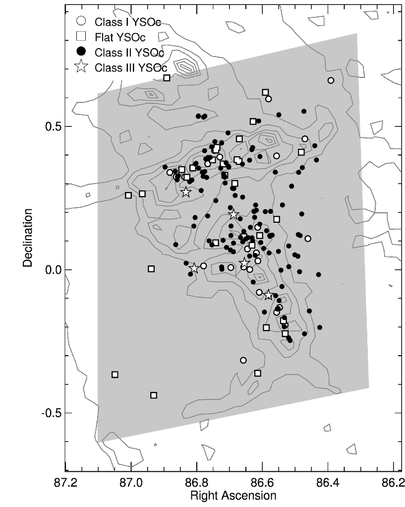
Figure 1: Spatial distribution of the YSO candidates as a function of Lada classes over-plotted on the contours from the VISTA extinction map (solid lines). The contour levels of extinction (A_K) are from 0.01 to 2 mag, in steps of 0.2 mag. The shaded area displays the regions observed with VISTA (tile no. 12).

Table 1: Filter central wavelength, saturation limit, limiting magnitude at the 5$\sigma$ level and completeness limit for the photometry of sources in tile no. 12 (L1630 N).

Filter	$\lambda_{C}$	Saturation	Mag5σ	Completeness
	($\mu$m)	limit		limit
$Z$	0.877	13.5	22.5	22.3
$Y$	1.020	12.0	21.1	21.5
$J$	1.252	11.0	20.3	20.5
$H$	1.645	11.0	19.3	19.5
$K_{S}$	2.147	10.0	18.5	18.5

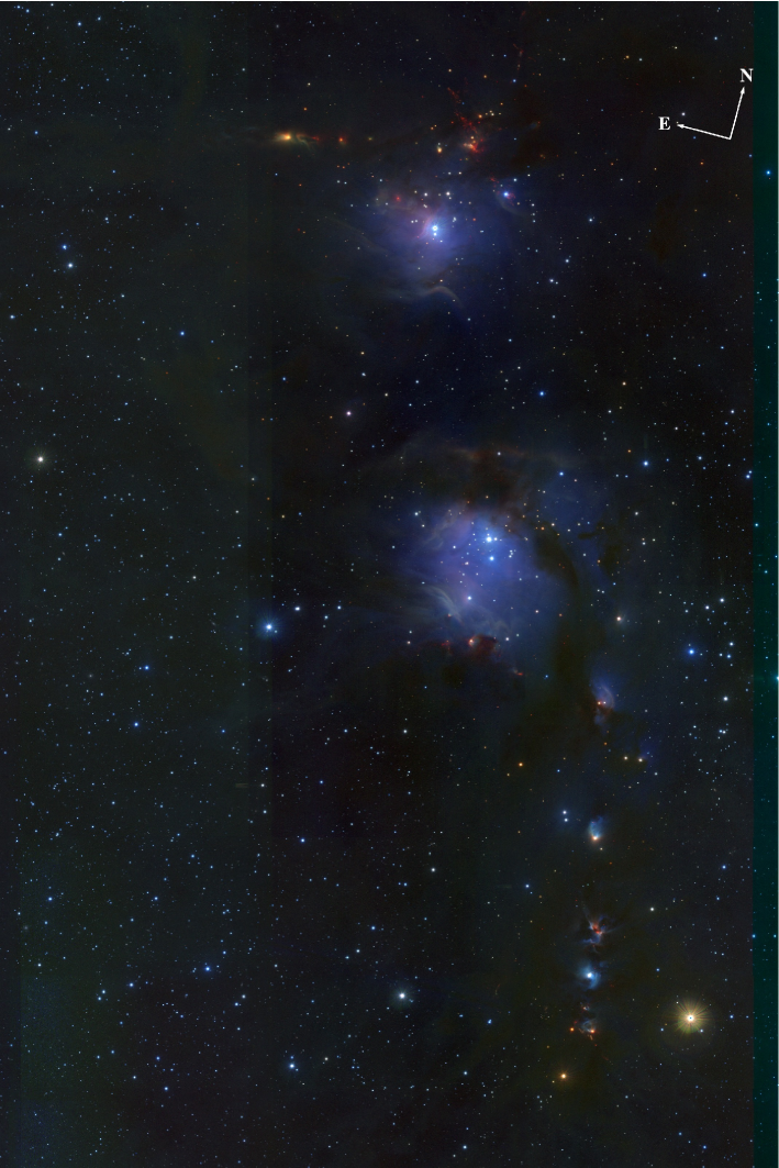
Figure 2: VISTA three colour (ZJKs) mosaic image of L1630 N on a logarithmic display. The image covers the grey shaded area of Figure 1.

The data reduction was performed by a dedicated pipeline, developed within the VISTA Data Flow System (VDFS), and run by the Cambridge Astronomy Survey Unit (CASU). The pipeline delivers science-ready stacked images and tiles, as well as photometrically and astrometrically calibrated source catalogues (Irwin et al., 2004). A total of $\sim$3.2 million sources were detected in the VISTA Orion Survey, and $\sim$155000 in tile no. 12 used for this work. The catalog also provides, for each source in each filter, a morphological parameter (FLAG) equal to $-1$ for point-like sources, $1$ for extended sources, $-2$ for borderline point-like sources, and $-7,-9$ for problematic detections, e.g. sources partly saturated or whose magnitude is contaminated by bad-pixels inside the aperture used for the photometry extraction, or truncated because the source is very close to the mosaic borders. The astrometric accuracy in the source catalog is $\sim 0\aas@@fstack{\prime\prime}2$ with respect to the UCAC4 catalog (Zacharias et al., 2013). Stellar sources typically show a FWHM of $0\aas@@fstack{\prime\prime}6-0\aas@@fstack{\prime\prime}8$. The instrumental magnitudes are obtained through aperture photometry and calibrated onto the VISTA system via non-saturated 2MASS stars in the field. Absolute photometric uncertainties are below 5% and the 5$\sigma$ limiting magnitudes, completeness and saturation limits in each filter are listed in Table 1 for the specific case of tile no. 12. The achieved magnitude limits in $JHK_{S}$ are $\sim$3 mag deeper than 2MASS. The approximate completeness limit in each filter was derived as the point where the histogram of the magnitudes (Fig. 3) diverges from the dotted line, which represents the linear fit to the logarithmic number of objects per magnitude bin, calculated over the intervals of good photometric accuracy (Santiago et al., 1996; Wainscoat et al., 1992). In order to estimate stellar mass limits from our saturation and completeness limits, we compare with the theoretical isochrones by Baraffe et al. (1998) and Chabrier et al. (2000). Since the isochrones are provided for the Johnson-Cousins photometric system, which is different from the VISTA photometric system, we converted them to the VISTA photometric system as described in Appendix A. We estimate that our survey should have detected, for a population as young as $\sim$2 Myr at a distance of about 400 pc (i.e., the case of L1630 N) essentially all objects from $\sim$1 M_⊙ down to $\sim$5 Jupiter masses ($\sim$0.0045 M_⊙) in a region showing less than 1 mag of visual interstellar extinction.

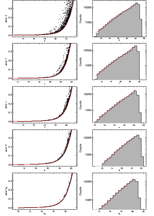
Figure 3: Left panels: Photometric errors as a function of magnitudes and relative exponential fit (continuous line) for non-saturated sources detected by the VISTA Orion Survey tile no. 12 in the $ZYJHK_{S}$ filters. Right panels: Number of detection as a function of magnitude. The line shows the linear fit to the logarithmic number distribution of magnitudes, which is used to find the turning point of the distribution, indicating our completeness limit.

2.2 Spitzer data

The Orion clouds were observed by the Spitzer Space Telescope (Fazio et al., 2004; Rieke et al., 2004) as part of the Guaranteed Time Observation (GTO) programs PID 43, 47, 50, 58, 30641, and 50070. The extraction of point source photometry from this survey in the four IRAC bands and the MIPS 24$\mu$m band and an overview of the basic properties of the resulting point source catalog have been presented by Megeath et al. (2012). The catalog contains 298405 sources that are detected in at least one of the IRAC bands or in the MIPS 24$\mu$m band, the limiting magnitudes at the 10$\sigma$ level are roughly 16.5, 16.0, 14.0, 13.0 and 8.5 at 3.6, 4.5, 5.8, 8 and 24 $\mu$m, respectively (see Fig. 2 by Megeath et al., 2012). The catalog exhibits spatially varying completeness due to confusion with nebulosity and crowding of point sources in dense clusters (see Fig. 3-4 by Megeath et al., 2012). The Orion IRAC/MIPS maps are broken into several fields centered on the regions of strong ${}^{13}\mathrm{CO}$ emission (Miesch & Bally, 1994). We used a sub-set of the general catalog covering an area of 2.58 deg² around L1630 N.

3 Selection of YSO candidates

The $J-H$ vs. $H-K_{S}$ color-color (CC) diagram is traditionally used to select low-mass YSO candidates (YSOc) on the basis of near-IR data, because young K/M type stars exhibit a narrow range of colors in this diagram and, in particular, an $H-K_{S}$ excess mainly arising from their circumstellar disk and/or in-falling envelope (Meyer et al., 1997; Luhman & Rieke, 1999; Lee et al., 2005). However, near-IR colors of YSOs may be mimicked, to some extent, by highly reddened stellar photospheres of older main-sequence dwarf stars in the field and, hence, the selected sample might be contaminated. On the other hand, the identification of YSOs on the basis of mid to far-IR colors alone is not trivial, because the YSO colors in this wavelength regime are very similar to those of many background galaxies (Sect. 3.1 by Evans et al., 2009). Thus, to select YSOs in L1630 N we adopt the approach by Harvey et al. (2007a), based on the combined use of $JHK_{S}$ photometry and Spitzer IRAC/MIPS colors. By using Spitzer observations of the Serpens star forming region and the SWIRE catalog of extragalactic sources (Lonsdale et al., 2003), these authors defined the boundaries of the disk-bearing YSO locus in several IRAC/MIPS color-magnitude and CC diagrams. Their criteria have proven to provide an optimal separation between disk-bearing YSOs (mainly class II, class I and Flat Spectrum objects), reddened field stars and galaxies, with the fraction of remaining contaminants (mainly background field dMe dwarfs, a few K/M-type giants, and Be and AGB stars) estimated to be around 30% (e.g., Spezzi et al., 2008; Oliveira et al., 2009; Cieza et al., 2010). These criteria have been applied to select YSO candidates in all star forming regions observed within the frame of the Spitzer c2d (Evans et al., 2009) and Spitzer Gould Belt Legacy surveys (e.g., Spezzi et al., 2011; Hatchell et al., 2012; Dunham et al., 2013).

We first matched our VISTA catalog for tile no. 12 with the Spitzer catalog by Megeath et al. (2012) using a matching radius of 3$\arcsec$, larger than the astrometric accuracy of our mosaics (Sect. 2.1) and corresponding to twice the typical FWHM of sources in IRAC maps. Then, we applied the YSO selection method by Harvey et al. (2007a) to the matched catalog, containing $\sim$58500 sources with complete $ZYJHK_{S}$, IRAC 3.6, 4.5, 5.8 and 8 $\mu$m and MIPS-24 $\mu$m photometry. A detailed review of the selection method can be found in Harvey et al. (2007a, b). Briefly, the selection method consists in the definition of an empirical probability function which depends on the relative position of a given source in several CC and CM diagrams, where diffuse boundaries have been determined to obtain an optimal separation between YSOs and galaxies. Figure 4 (left panels) shows the VISTA/Spitzer CC and CM diagrams used to select the YSO candidates in L1630 N. Note that the method requires detection in all IRAC bands and in MIPS-24 $\mu$m with a S/N higher than 3 to classify an object as a YSO candidate or a background galaxy. Diskless YSOs, i.e. class III sources, are usually rejected by the selection method. Moreover, older field objects with no IR excess emission are rejected a priori because their IR colors are comparable with normal photospheric colors, e.g., $K_{S}-[4.5]<$-0.1, [8]-[24]$<$0.1, [4.5]-[8]$<$0.2 (Harvey et al., 2007b). In addition to the criteria by Harvey et al. (2007a), we used the VISTA morphological parameter (FLAG; Sect. 2.1) to distinguish between point-like (FLAG=-1) and extended (FLAG=1) YSO candidates; YSO candidates truncated and/or contaminated in VISTA pass-bands (-9$\leq$FLAG$\leq$-2) could not be classified. We note that, although clearly extended sources in the VISTA mosaic are more likely to be galaxies, we can not exclude them a priori, because YSOs still surrounded by significant circumstellar material might appear fuzzy/extended at IR wavelengths. Thus, we establish the YSO or galaxy nature on the basis of the above mentioned probability function alone, which depends exclusively on the VISTA/Spitzer colors of the sources.

We find 188 YSOc in L1630 N, shown in Figure 4 (left panels) as red dots, squares and asterisks for point-like, extended and morphologically unclassified sources, respectively.

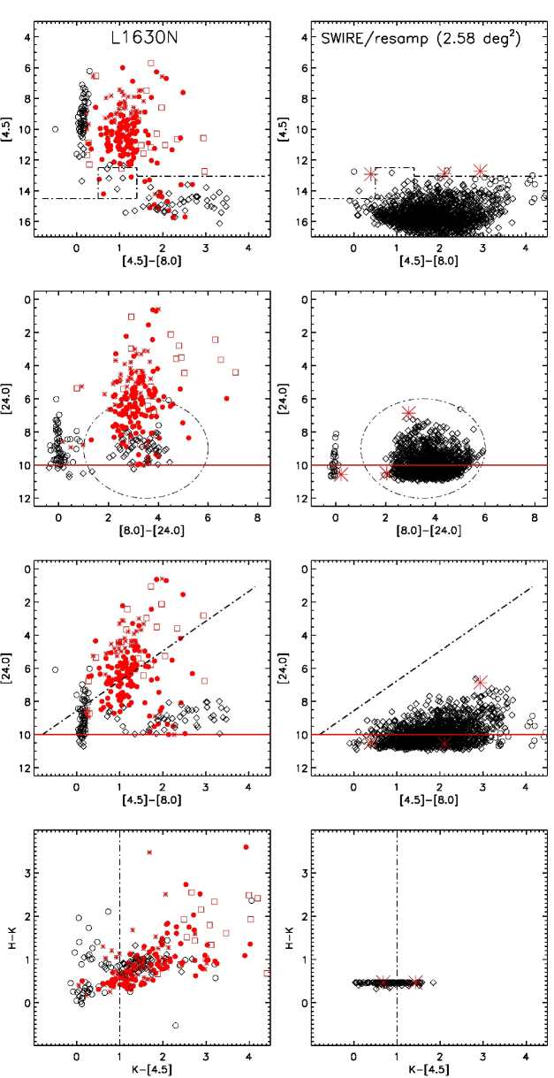
Figure 4: Left panels: VISTA/Spitzer CM and CC diagrams for L1630 N. The dot-dashed lines show fuzzy limits with exponential cutoffs that define the YSO candidate selection criterion in the each diagram, excluding contamination from galaxy (diamonds) and field stars presenting normal photospheric colors (circles). The continuous lines show hard limits, objects fainter than which are excluded from the YSO category. Point-like and extended YSO candidates are indicated by dots and squares, respectively; YSO candidates with no VISTA morphological classification are indicated by asterisks. Right panels: 2MASS/Spitzer CM and CC diagrams for the SWIRE catalog (Sect. 3.1). Symbols are as in the left panels. Three objects of the SWIRE catalog (marked as asterisks) are classified as YSOc according to our selection criteria.

3.1 On the contamination of the YSOc sample

We adopted a statistical method to distinguish YSOs from extragalactic contaminants and field stars, hence, our candidates sample could be still slightly contaminated.

The number of interloping stars can be probed by using analytic models of the Galactic stellar distribution, i.e., simulations of the expected properties of stars seen towards a given direction of the Galaxy over a given solid angle. We performed this exercise by using the Galaxy model by Robin et al. (2003) and their online tool. In the temperature range of our candidates, foreground stars are expected to be main-sequence cool dwarfs, whereas red giants are expected to dominate the background population. Assuming a cluster distance of 400 pc and a typical extinction of A_V$\approx$1 mag due to the L1630 N cloud itself, we expect some 50 foreground dwarfs in the 1$\times$1.5 square degree area observed in by VISTA (tile n. 12) with apparent $K_{S}$ magnitude between 7 and 18.5 and spectral types of M0 to M9, i.e., the magnitude and spectral range corresponding to members of L1630 N detectable by our survey ($\lesssim$1 M_⊙; Sect. 2.1). Only a handful ($\sim$3) of background giants are expected to be found in the locus occupied by the cluster members because they generally appear much brighter than L1630 N members in the same effective temperature range. We thus conclude that only foreground cool main-sequence stars can contribute noticeably to the contamination of our candidate sample, but the contamination level is at most 25-30%. We note that contamination is higher ($\sim$50%) in the substellar regime ($\sim$0.1 M_⊙, i.e., K${}_{S}\approx$13 mag), and lower in the stellar regime ($\sim$20%). On the other hand, as seen in Figure 1, the YSOc very clearly follow the cloud extinction contours which is not expected for a randomly distributed foreground population. Also, we find almost all of our YSOc consistent with infrared excess sources of class II or earlier (see Sect. 5). Therefore, we conclude that the true contamination of our sample is very low.

In order to have a statistical estimate of possible remaining extragalactic contaminants, we used the Spitzer Wide-area Infrared Extragalactic (SWIRE Surace et al., 2004) catalog coming from the observations of the ELAIS N1 field (Rowan-Robinson et al. 2004). The SWIRE catalog was trimmed and resampled as accurately as possible to match the spatial extent (2.58 deg²) and sensitivity limits (Sect. 2.2) of the Spitzer observations in L1630 N. Moreover, the photometry of sources in the SWIRE catalog was edited in order to simulate the interstellar extinction in the direction of L1630 N, as expected on the basis of the VISTA extinction map (Sect. 7.1). $JHK_{S}$ for the SWIRE sources are recovered from the 2MASS catalog (Skrutskie et al., 2006). For further details on how the trimmed resampled SWIRE comparison catalog was created, we refer the reader to Evans (2008) and Harvey et al. (2007a). The selection criteria applied to the comparison resampled SWIRE data lead to the conclusion that only 3 (i.e., less than 2%) of the selected YSO candidates in L1630 N may be background galaxies (Fig. 4). This result is similar to what Harvey et al. (2007a) and Alcalá et al. (2008) found for the Serpens and Cha II molecular clouds, respectively. Indeed, all the 188 candidates have been visually inspected in the VISTA images and we find that only two of them are clearly galaxies; these two candidates have been neglected in the subsequent analysis. All the remaining 186 candidates appear point-like or almost point-like in all our images and their photometry is not contaminated by nearby saturated stars, or any other artifact that might affect our selection criterion. A few of them ($\sim$3%) present a close companion in the VISTA images not resolved in the Spitzer images and, hence, their Spitzer fluxes might be contaminated. We can not discharge a priori these candidates, because one or both objects in the system might still be young and, hence, responsible for the observed IR excess emission.

This leads us to a remaining caveat in our selection method. Our YSO candidates might be members of binary/multiple systems too close to be resolved with VISTA/Spitzer and, hence, affecting the measured photometry. As seen in Sect. 2.1, our candidates are expected to have masses $\lesssim$1 M_⊙. The multiplicity fraction for stars in this mass regime is estimated to be between 20% and 40%, depending on the actual mass of the primary star and the separation range (Duquennoy & Mayor, 1991; Mason et al., 1998; Basri & Reiners, 2006; Lada, 2006). However, higher resolution imaging or spectroscopy would be needed to assess the actual multiplicity fraction in L1630 N.

3.2 Comparison with previous surveys

Before our study, a census of the young stellar population in L1630 N was presented by Flaherty & Muzerolle (2008) and by Fang et al. (2009). Flaherty & Muzerolle (2008) identified 69 cluster members with a rather spread spatial distribution, i.e., not confined to regions of dense gas and dust. For 67 of these members, they derived accurate spectral type and luminosity and estimated a median age of 2 Myr, and a large fraction of stars with infrared excess actively accreting (79%). Using a mix of criteria (presence of H$\alpha$ emission, Li I absorption or IR excess) Fang et al. (2009) selected and analized 132 PMS stars in the general direction of the clusters. This list includes practically all the PMS stars studied by Flaherty & Muzerolle (2008). For 111 stars Fang et al. (2009) provide a classificaton in terms of their IR-excess as ”thick disk, transitional disk, thin disk and no disk”. Most of the 21 objects missing IR classification lack any information on Li I absorption and were selected as PMS stars by Fang et al. (2009) only because H$\alpha$ is detected in emission, although rather weak considering their spectral types (White & Basri, 2003).

Our YSOc sample consists of 186 objects. In Table A we report their coordinates and VISTA + Spitzer photometry. The VISTA/Spitzer selection criteria recovered 50 out of the 69 (i.e. $\sim$75%) PMS stars listed by Flaherty & Muzerolle (2008), specifically 10 weak T Tauri stars (WTTs) and 40 classical T Tauri stars (CTTs). Likewise, our criteria recover 82 of the 132 objects in Fang et al. (2009) (i.e., $\sim$62% of the whole sample, but 74% of the sample with IR classification). Most of the recovered objects by the VISTA/Spitzer selection criteria in both catalogs can be classified as Class II YSOs. Our survey missed about 50 of the previously known YSOs in the area, i.e. $\sim$21% of the YSO population (50 of 186+50), the vast majority of which are WTTs or objects without disks, i.e. Class III YSOs. We mark in Table A the YSOc already identified by Flaherty & Muzerolle (2008) and/or Fang et al. (2009).

Although the selection criteria and color cuts presented here are different from those by Megeath et al. (2012) it is also interesting to compare our results with their selection, since we gathered the Spitzer photometry from their catalog (see Section 2.2). In our studied area there are 257 sources selected by Megeath et al. (2012) as possible YSOs, but 75 of these lack information in at least one IRAC band or at 24 $\mu$m. Since our selection criteria require the detection in all IRAC bands and at 24 $\mu$m, we can classify 182 of the Megeath et al. (2012) sources in the region. With our methods we thus recover 162 YSOs, meaning that our criteria miss 20 of the Megeath et al. (2012) sources. Most of them are classified as possible protostar candidates by Megeath et al. (2012) and are distributed in regions of high sellar density. Thus, our criteria recover about 90% of the Megeath et al. (2012) sources.

4 Luminosity Function and Characteristic Stellar Mass

The stellar luminosity can be used as a poor but still useful first-order proxy for mass, assuming that most of the stars have formed more or less at the same time. Before using the range of luminosities to provide an estimate of the mass range, we determined the degree of completeness of the YSO candidate sample in L1630 N. Our selection criteria ultimately rely on the VISTA and Spitzer IRAC 3.6-8$\mu$m/MIPS 24$\mu$m detection of the objects and on the quality of this detection. Thus, in order to investigate the expected number of low-luminosity objects and infer the typical mass distribution of our YSOc sample, we have to take the completeness of these two datasets into account.

4.1 1-30$\mu$m Bolometric Luminosity Function

In order to estimate the completeness of the Spitzer observations in the L1630 N, we used the same approach as Harvey et al. (2007a), which has been applied to all c2d/GB clouds (e.g., Alcalá et al., 2008; Merín et al., 2008; Spezzi et al., 2011).

We derive first the total infrared luminosity of our YSOc by integration over their SED flux between 1 to 30 $\mu$m; the total flux was converted to luminosity assuming a distance of 400 pc. We then applied the Harvey et al. (2007a) completeness correction factors for the c2d survey to our YSO candidate samples. Harvey et al. (2007a) estimated the completeness of the c2d catalogs by comparing, for each luminosity bin, the number of counts from a trimmed version of the deeper SWIRE catalog of extragalactic sources (assumed to represent 100% completeness by c2d standards) with the number of counts for the c2d catalogs in Serpens. This completeness correction can be applied to our Spitzer catalog of L1630 N because its photometric depth (Sect. 2.2) is similar to the one of the c2d catalogs (in both cases the 10$\sigma$ limit is $\sim$16.5 mag for IRAC 3.6$\mu$m and $\sim$8.5 mag for MIPS 24$\mu$m; compare Fig. 23 and 26 by Evans (2008) with Fig. 2 by Megeath et al. (2012)). Figure 5 shows the 1-30$\mu$m bolometric luminosity function (BLF) for YSOc in L1630 N before (solid line) and after (dashed line) correction for completeness, and suggests that we are missing only a few ($<$5) of additional low-luminosity sources with $log(L/L_{\odot})<-1.7$. These objects have been missed by our selection either because they are below the noise level of the Spitzer observations or because they are located within the galaxy loci of the CM diagrams (Fig. 4). In conclusion, our YSO candidate samples in L1630 N is fairly complete. The luminosity histogram suggests a completeness better than $\sim$95% at luminosities down to 0.01 L_⊙, which correspond to a mass of 0.02 M_⊙ for 2 Myr old stars according to the PMS evolutionary tracks by Baraffe et al. (1998) & Chabrier et al. (2000). The peak of the luminosity function appears at 0.25 L_⊙, which corresponds to a 0.4 M_⊙ star (i.e., spectral type M3 at an age of 2 Myr). A very peculiar characteristics of the L1630 N 1-30$\mu$m bolometric luminosity function is that it shows a significant number ($\sim$35%) of low- and very low-luminosity objects ($log(L/L_{\odot})\lesssim-1$). A similar tail of low-luminosity objects was noted in the Lupus I, III and IV star forming regions ($\sim$40% Merín et al., 2008; Comerón, 2008), while it is not observed in other c2d/GB clouds such as Cha II ($\sim$15% Alcalá et al., 2008), Lupus V and VI (10-20% Spezzi et al., 2011) and Serpens (Harvey et al., 2007a).

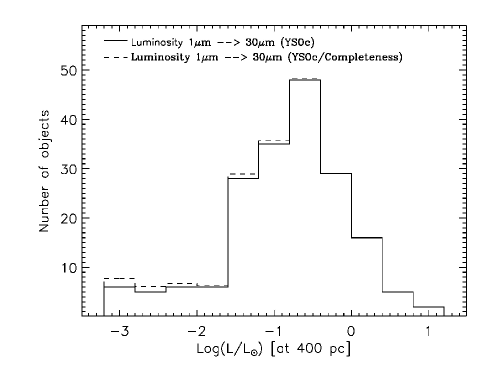
Figure 5: Luminosity distribution for the YSOc in L1630 N (solid histogram). The plotted luminosities were determined as in Harvey et al. (2007a), i.e., by integration of the SEDs from 1 to 30 $\mu$m. The corrected luminosity distribution, determined by applying completeness factors at each luminosity bin as in Harvey et al. (2007a), is over-plotted (dashed histogram).

4.2 K-band Luminosity Function

To further investigate/confirm the stellar mass distribution of the L1630 N YSO population, we also constructed its $K$-band luminosity function (KLF). We choose the KLF rather than the $J$ or $H$-band luminosity functions in order to minimize the effects of extinction, to maximize our sensitivity to intrinsically red, low-luminosity members of this cluster, and to make detailed comparisons to the KLF of the nearby Trapezium cluster presented by Muench et al. (2002). We did not correct the K-band fluxes for excess emission, but this should not affect the comparison with the Trapezium Cluster KLF, because Muench et al. (2002) do not correct for disk excess flux neither. The majority of stars in the Trapezium sample are disk-sources, and the H-K color distribution of the whole Trapezium sample is very similar to the H-K color distribution of our YSO sample in L1630, indicating a similar disk excess nature for the samples.

In Figure 6 we present the observed and dereddened KLF of L1630 N. We use relatively wide bins (0.5 mag) that are much larger than the photometric errors (Fig. 3) and adopt for each YSOc the visual extinction derived from the VISTA extinction map (Sect. 7.1) and reported in Table A. The K-band excess could add $\sim$0.5mag, on average, to the observed K-band magnitude (Meyer et al., 1997), i.e. about the same size as the KLF binsize. However, this does not have any significant affect on our conclusions on the KLF shape, as the excess is a property over the entire luminosity range (i.e. there is no singular effect on an individual mass regime of the KLF), and the steady decline in the sub-stellar regime discussed below is a robust result. We also indicate in Figure 6 the $K$-band saturation limit and limiting magnitude of our VISTA catalog (Table 1) and overplot, for comparison purposes, the Trapezium KLF as derived by Muench et al. (2002), arbitrarily scaled to the peak of the L1630 N KLF.

The KLF of L1630 N shows a broad peak between 10.5 and 12 mag, i.e., 0.3-0.7 M_⊙ at the cluster distance and age according to the 2 Myr isochrone by Baraffe et al. (1998) & Chabrier et al. (2000) converted to the VISTA photometric system (Appendix A). Then, it steadily declines to the Hydrogen-burning limit ($\sim$0.1 M_⊙, i.e., K${}_{S}\approx$13 mag). Below this limit, we count a fraction of 28% substellar YSOs. However, we note that the expected contamination from field stars mimicking the colors of BDs is expected to be $\sim$50% (Sect. 3.1), while it is lower in the stellar regime ($\sim$20%) and, hence, the actual fraction of sub-stellar objects in L1630 N could be as low as 20%. Thus, the KLF of L1630 N indicate a stellar mass distribution consistent with the 1-30$\mu$m BLF. Moreover, it appears remarkably similar to the Trapezium KLF (see Fig. 11a by Muench et al., 2002), which presents a broad peak around 0.6 M_⊙ and then declines into the sub-stellar regime, the fraction of sub-stellar objects being $\sim$22%. Muench et al. (2002) also reported a significant secondary peak around 10-20 Jupiter masses ($\sim$0.02 M_⊙). Although we do observe a similar fraction of sub-stellar objects, the presence of this secondary peak is not obvious in the KLF of L1630 N, which appears to keep its steady decline down to our completeness limit ($\sim$0.0045 M_⊙, i.e., K${}_{S}\approx$18.5 mag).

The mass function shape of the Trapezium cluster in the sub-stellar regime has been long debated, because the large fraction of brown dwarfs (BDs) with respect to other nearby star forming regions ($\sim$15%; Briceño et al., 2002; López Martí et al., 2004; Spezzi et al., 2007, 2008, 2009) could be an affect of spatial and photometric incompleteness of the surveys conducted so far. However, more and more complete surveys are now available and, still, there is no universal agreement on the behavior of the mass function over the substellar regime. For a complete collection of BD fraction measurements in nearby star forming regions and a discussion on possible trends, we defer the reader to Scholz et al. (2012) and references therein. Note that these authors compare the star-to-BD ratio (R_star/BD) for various star-forming region (see their table 5). It appears more and more evident that, on one hand, there are clusters like IC 348, T association like Taurus, Chamaeleon, $\rho$-Ophiuchus, etc., with a low number of sub-stellar objects (R_star/BD in the range 5 to 8), and on the other hand there are more massive clusters such as Trapezium, the Orion Nebula Cluster (ONC), NGC 1333, Upper Scorpius, etc., where this number is much higher (R${}_{star/BD}\approx$ 2-4). L1630 N, as other clusters in the Orion complex (Trapezium and the ONC), would belong to this last category, with R${}_{star/BD}\approx$2.5-3.9 depending on the actual contamination level. The variation of the fraction of substellar objects observed from region to region possibly indicates environmental effects on their formation mechanism, a key point of the current star formation theory still under debate (e.g., Whitworth et al., 2007).

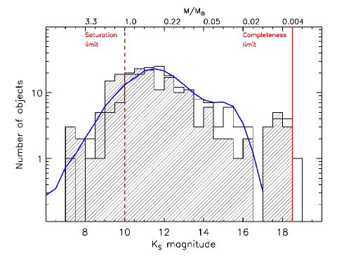
Figure 6: The L1630 N $K$-band luminosity function (KLF) before (empty histogram) and after correction for interstellar extinction (line-filled histogram). The labels in the top x-axis indicate the corresponding stellar mass according to the VISTA 2 Myr isochrone (Appendix A). The continuous and dashed vertical lines indicate the completeness and the saturation limit of the VISTA $K$-band photometry, respectively. The continuous curve is the KLF of the Trapezium cluster (Muench et al., 2002), scaled to the peak of the L1630 N KLF.

5 Lada classes, disk fraction and disk lifetimes

In this section we revise the disk properties of the young stellar population in NGC2068/2071 on the basis of our YSO candidates sample, and in comparison with the results by Flaherty & Muzerolle (2008).

In order to investigate the disk properties of our YSO candidate sample, we adopted the Lada classification (Lada & Wilking, 1984) based on the SED slope ($\alpha$) of the line joining the flux measurements at 2.2 $\mu$m (K-band) and MIPS-24 $\mu$m. In particular, we used the Lada’s class separation as extended by Greene et al. (1994), i.e. $\alpha\geq 0.3$ for Class I, $-0.3\leq\alpha<0.3$ for flat-spectrum sources, $-1.6\leq\alpha<-0.3$ for Class II sources, and $\alpha<-1.6$ for Class III sources. We report in Table A the Lada class computed for each YSOc and give in Table 2 the statistics for the entire YSOc sample in L1630 N. As shown in Figure 7, the dominant objects in L1630 N are those of Class II (68%), followed by flat-spectrum (16%) and Class I (13%) sources, with only a minority being Class III sources (3%). The distribution of YSOs over class supports the young age estimated for this star-forming region. The ratio of the number of Class I and flat-spectrum sources to the number of Class II and Class III sources is 0.42, similar to the ratio measured in Serpens (Harvey et al., 2007a) and other clouds of similar age surveyed by the Spitzer c2d survey (Evans et al., 2009). The total observed fraction of objects with thick disks and/or envelope (Class I to II) for our sample is on the order of 97%, while those with thin or no disk (Class III) represents only $\sim$3% of the sample. The total disk fraction is considerably higher than the values derived in other regions of similar age (e.g., in IC 348; Lada, 2006) and this would make L1630 N a clear outlier with respect to the typical disk fraction vs. age trend (e.g., see Fig. 1 and Fig. 4 by Haisch et al., 2001; Fedele et al., 2010, respectively).

Table 2: Summary of Lada Classes in L1630 N and estimated lifetime for each phase.

Lada class	n. of YSO candidates	lifetime
		(Myr)
I	25 (13%)	0.40
Flat	30 (16%)	0.48
II	126 (68%)	2†
III	5 (3%)	–

^† Assumed lifetime for the Class II phase (Evans et al., 2009).

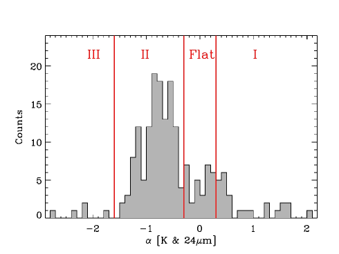
Figure 7: $\alpha$-slope distribution of YSOc in L1630 N. The vertical lines indicate the intervals defining the four Lada classes. The populations is largely dominated by Class II objects.

Contamination from field stars, which could be as high as 25-30% (Sect. 3.1) should not heavily affect the relative number of object with and without disk, because there is no reason to assume that this kind of contamination affects one Lada class more than the others. Background galaxies preferentially mimic the colors of YSOs with thick disks/envelope, but they may account for 2% of our YSOc sample at most and can not justify the high number of Class I to II objects.

However, one may wonder whether our census might have missed a significant number of diskless YSOs. This would be possible because the c2d criteria select only IR excess objects. A direct way to investigate the number of diskless YSOs missed in our survey is to compare our results with those of deep X-ray observations, which are the most secure way to trace the population of class III objects. By the merging of many Chandra pointed observations in a region centered between NGC 2068 and HH24-26, Principe et al. (2014) obtained a very deep X-ray image with an equivalent exposure time of about 240$\times$10³sec. In an area of about 0.12 square degrees they detected 52 X-ray sources, 32 of which can be identified with class III or transition objects. Six of these objects have been recovered in the same area by our selection, but five were classified as Class III and one as Class II by our work. Considering that transition objects may mimic colors of Class III objects, the conclusion is that our selection misses a factor of about 5 or 6 the actual number of diskless YSOs. This is in perfect agreement with the estimated number of missed diskless YSOs in the c2d surveys (see Sect. 3.2 in Evans et al., 2009). Hence, we are most likely missing 25-30 class III YSOs (i.e. $\sim$20%) in our sample (see Table 2), which is also consistent with the fraction of diskless YSOs missed by our criteria in the Flaherty & Muzerolle (2008) and Fang et al. (2009) samples (see Sect. 3.2). Certainly, in order to obtain a real full census of class III objects in the area a much larger scale deep X-ray survey would be needed. But since such observations are currently not available we use the above correction as a first order estimate, which leads to an expected fraction of class III YSOs in L1630 N predicted by our data of $\sim 15$%. This is still lower than expected on the basis of a cluster age of 1-2Myrs.

The surveys for PMS objects by Flaherty & Muzerolle (2008) and Fang et al. (2009) produced a similar result on the high fraction of YSOs with disks and envelopes. Their surveys are rather complete in both space and flux and are based on different selection criteria, i.e., location on optical/near-IR color-magnitude diagram with respect to the expected position of the main sequence at the cluster distance and subsequent spectroscopic follow-up. Flaherty & Muzerolle (2008) report a fraction of strong disk (Class I/II) of 66% and a fraction of MIPS-weak disks of 16%, in perfect agreement with our fraction of disk objects after applying the correction of missed class III sources. They also find a fraction of IRAC-weak disks (Class III) of 20$\pm$8%, higher than our estimate but still lower than the fraction of Class III YSOs found in regions of similar age. Similarly, Fang et al. (2009) report a high fraction ($\sim$80%) of disks in the region, although this value might also be biased by their selection which preferentially selects disk bearing young stars.

Alternatively, the substantial number of objects in younger SED classes is due to still ongoing star formation in L1630 N, and correspondingly young age ($\leq$ 1 Myr) for the studied YSO samples. As we will see in Sect. 7.3, some studies (Lada et al., 2010; Heiderman et al., 2010) have revealed that, if most of the present-day mass measured for a given cloud lies below a certain gas surface density threshold, which was determined by Heiderman et al. (2010) to $\sim 129\,\mathrm{M}_{\odot}\,\mathrm{pc}^{2}$ (corresponding to $\mathrm{A}_{\mathrm{V}}\approx 8.6$ mag), a decrease in star formation could plausibly be caused by exhaustion of gas above such a threshold in surface density. Spezzi et al. (2011) demonstrated that this is the case for some clouds in the Lupus complex (Lup V and VI), where only $\sim$1% of the cloud mass lies above the threshold and, consistently, older SED classes (Class III) dominate the YSO population, while other Lupus clouds with 5 to 25% of the cloud mass above the threshold are mainly populated by younger SED classes (Class I to II). The fraction of cloud mass above the threshold in L1630 N is $\sim$35% (Table 4), i.e., even higher than in the most active star-forming region of Lupus (Lupus III), and may explain its exceptionally high disk fraction.

Thus, although the actual value might be slightly lower, the result on the high disk fraction in L1630 N seems to be real. The average disk fraction vs. age trend reported in the literature (e.g., Fedele et al., 2010) suggests a median disk lifetime around 2-3 Myr, meaning that $\sim$50% of the stars in a given population should have lost signatures of their disks after this time. However, several cases of clear outliers with respect to the average disk fraction vs. age trend have been reported in the literature. For example, Alcalá et al. (2008) found that only about 20%-30% of YSOs in Chamaeleon II have lost their primordial disks in about 4 Myr (i.e., the average age for its members), and Sicilia-Aguilar et al. (2006, 2013) measured a disk fraction of $\gtrsim$50% in the coeval cluster Trumpler 37. Moreover, studies in NGC 3603 (Beccari et al., 2010) and the Magellanic Clouds (Spezzi et al., 2012; De Marchi et al., 2011a, b) indicate that a considerable fraction of PMS stars still exhibit signatures of accretion from a circumstellar disk at ages as old as 10 Myr. It is still under debate whether these differences from region to region are due to residual incompleteness effects of different surveys, limitations of the adopted selection methods, etc., or to the specific properties of the given star-forming environment (such as metallicity, presence of strong UV radiation fields, multiplicity, crowding, etc.), which may strongly affect disk evolution (e.,g., Hollenbach et al., 2000; Linsky et al., 2007; Dullemond & Dominik, 2005; Johansen et al., 2009; Daemgen et al., 2013).

Evans et al. (2009) derived the half-life for each of the Lada classes from the combined analysis of the Spitzer c2d data set. According to this study, the half-life for Class II sources is $\sim$2 Myr. If star formation has been continuous over a period longer than the age of Class II sources, the lifetime for each phase can be estimated by taking the ratio of number counts in each class with respect to Class II counts and multiplying by the lifetime for Class II. According to the statistics of Lada classes in L1630 N, we estimate a lifetime of 0.4 and 0.48 Myr for the Class I and Flat-spectrum phase, respectively (Table 2). These values agree with the lifetimes derived by Evans et al. (2009) by averaging all c2d clouds.

Table 3: Results of the clustering analysis and properties of star formation in sub-structures in Lynds 1630 N

Region	#YSOs	# IR Class				Mass	$\langle A_{V}\rangle$	SFE	Area	Mass/Area ($\Sigma_{gas}$)	SFR/Area ($\Sigma_{SFR}$)
		I	Flat	II	III	(M⊙)	(mag.)	%	(pc2)	(M⊙ pc-2)	(M⊙ Myr-1 pc-2)
Extended	15	4	3	6	2	1840	0.3	0.4	…	…	…
Lynds 1630 N	171	21	27	120	3	2050	4.8	4.0	20.2	102	2.0
…NGC 2071	52	5	12	34	1	400	8.8	3.8	2.17	180	6.0
…NGC 2068	45	4	5	36	0	243	5.5	5.3	2.12	115	5.4
…HH24-26	14	6	2	5	1	124	7.7	3.3	0.77	161	4.6

6 Spatial Distribution and Clustering

The spatial distribution of the different classes of objects in L1630 N is shown in Figure 1 over-plotted on the VISTA extinction map, derived as explained in Sect. 7.1. The Class I and Flat sources coincide or are located close to the sites of highest extinction, as observed in all young clusters still associated with the residual parental clouds.

NGC 2068 and NGC 2071 are the most prominent star-forming clusters in the L1630 N molecular cloud. The VISTA extinction map shows, in a consistent way, two extinction peaks corresponding to the approximate center of NGC 2068 (R.A.$\approx$86.65 deg, Dec.$\approx$0.1 deg) and NGC 2071 (R.A.$\approx$86.75 deg, Dec.$\approx$0.35 deg). It is also evident that, beside these two peaks, there is an additional extinction peak centered at R.A.$\approx$86.55 deg and Dec.$\approx$-0.15 deg. This third peak corresponds to the HH 24-26 group of Herbig-Haro objects, and is very close to V1647 Ori (see Fig. 7 by Gibb, 2008), a low-luminosity protostar, perhaps in a transition phase from Class I to Class II which underwent a strong outburst in 2004 (Briceño et al., 2004). We also observe a very clear concentration of Class I and Flat sources around this peak, confirming that the region is one of the several small centers of star formation in L1630. Another argument for still actively ongoing star formation, is a notable concentration of presumably very young protostars in the region (see Stutz et al., 2013).

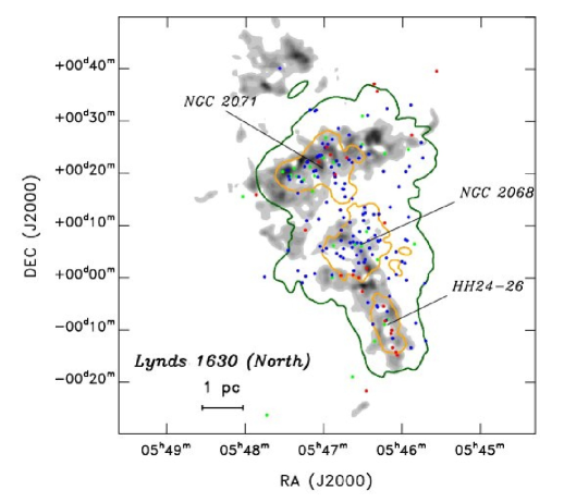
Figure 8: Distribution of young stellar objects plotted over the extinction map (in gray) of the region. The green and orange contours correspond to volume densities of 1 M_⊙ pc^-3 and 10 M_⊙ pc^-3, respectively. Class I sources are shown in red, Flat spectrum sources in green and Class II sources in blue.

Lada & Lada (2003) suggested that a cluster should be a group of some 35 members with a total mass density larger than $1\,\mathrm{M}_{\odot}\,\mathrm{pc}^{-3}$. To compare with this criterion and in order to assess the sub-clustering structures in L 1630, it is important to examine the distribution of YSOc in a quantitative and uniform way. We calculated the volume density of YSOs, based on their Lada classes and position, using a nearest neighbor algorithm similar to the one applied by Gutermuth et al. (2005) and implemented by Jørgensen et al. (2008) for the c2d clouds. The calculations assume that the distribution of sources is locally spherical. We applied the algorithm to the whole sample of 186 YSOs in Table A. The overall results, reported in Table 3, are shown in Figure 8.

To define a cluster the c2d surveys adopted the tighter level of 25 times the Lada & Lada (2003) criterion (i.e., a mass density of $25\,\mathrm{M}_{\odot}\,\mathrm{pc}^{-3}$), which normally provides the already established cluster and group boundaries. Within the c2d surveys, ”clusters” are regions with more than 35 YSOs within a given volume density contour and ”groups” are regions with less. The lowest number of YSOs that is considered to constitute a separate entity is 5. ”Clusters” and ”groups” can be either ”tight” or ”loose” depending on whether their volume densities, $\rho$, are higher than 25 or 1 M_⊙ pc^-3 (corresponding to 50 and 2 YSOs pc^-3), respectively, assuming an average YSO mass of 0.5M_⊙. As noted in the c2d papers, these criteria are useful as a way of making direct comparison between regions within clouds and across different clouds, but being empirical they should not be used as evidence for discussions on whether the star formation process is hierarchical or not.

In L1630 N we identify structures with two levels of volume densities, structures with a density larger than 1 M_⊙ pc^-3 (similar to the criterion for a cluster by Lada & Lada, 2003) or structures with a density as high as 10 M_⊙ pc^-3. Note, however, the latter is lower than what was applied for ”tight” associations in the c2d surveys. Thus, according to the c2d criteria, the loose clusters identified in this region are L1630 N as a whole with a density of 1 M_⊙ pc^-3 and NGC 2071 and NGC 2068 with a density of 10 M_⊙ pc^-3. The HH24-26 entity can be defined as a loose group with a density of 10 M_⊙ pc^-3.

7 Overall results on star formation in L1630 N

In this section we analyze and discuss the cloud properties of L1630 N and the global properties of star formation in this region on the basis of the VISTA observations and our YSOc sample. Our results are summarized in Table 4.

7.1 Extinction map, cloud mass and surface density

An extinction map, with a resolution of 30$\arcsec$, was constructed for the entire area of Orion observed in the VISTA SV mini-survey (Lombardi et al., in prep.). The technique used is optimized to produce highly accurate extinction maps from multi-band near-IR photometric data as outlined in Lombardi & Alves (2001, NICER) and Lombardi (2009, NICEST). The method is the natural generalization of the near-infrared color excess (NICE) method of Lada et al. (1994) and produces significantly less noisy and, hence, more accurate extinction maps taking advantage of all bands available. Applications of this technique to 2MASS data has shown an improvement with respect to the standard NICE algorithm of a factor 2 on the noise variance (Lombardi & Alves, 2001). We further compared our extinction map values with the spectroscopic values inferred by Flaherty & Muzerolle (2008) for a sample of 67 previously known PMS stars in the cloud and found a good agreement (within 2-3 visual mag), but also an apparent shift of A${}_{V}=3.4$mag (i.e. the extinction map gave a consistently higher A_V than what was determined from spectroscopy). This has been observed for other regions as well and can be explained by the fact that the extinction map measures the extinction through the whole cloud, while the PMS stars are located in the cloud.

According to this extinction map, the extinction in the L1630 N cloud (tile no.12) is typically low ($A_{V}\approx$1 mag), with peaks up to A${}_{V}\approx$20 mag occurring close to the following locations: R.A.=86.75 deg & Dec.=0.35 deg (i.e., the center of NGC 2071), R.A.=86.65 deg & Dec.=0.1 deg (i.e., the center of NGC 2068) and R.A.=86.55 deg & Dec.=-0.15, where a group of YSOc has been identified by us (Sect. 6).

Using the extinction map and assuming a distance of 400 pc, we also estimated the cloud mass for the L1630 N complex. To this aim we used the relationship between gas surface density, $\Sigma_{gas}$, and extinction by Heiderman et al. (2010), i.e. $\Sigma_{gas}\leavevmode\nobreak\ =\leavevmode\nobreak\ 15\leavevmode\nobreak\ \times\leavevmode\nobreak\ {\rm A_{V}}$ M_⊙/pc². We estimated that the total cloud mass for $A_{V}\geq 2$ mag is about 3865 M_⊙; considering that the area where A${}_{\rm V}\geq$2 mag extends over $\sim$39 pc², the cloud column density is about $\sim$100 M_⊙ pc^-2. The NICE and NICER methods provide an intrinsic error of about 0.5 mag, on the average. Assuming this value as the intrinsic error of our VISTA extinction map, and an error on the distance to the cloud of about 10% (see Sect. 2 in Gibb, 2008), we estimated that the cloud mass and column density of L1630 N can be safely placed in the ranges 3200$-$4600 M_⊙ and 81$-$116 M_⊙ pc^-2, respectively.

We stress that in $\sim$35% of the cloud area where $A_{\rm V}\geq 2$ mag the extinction is above 8.6 mag. As concluded in Heiderman et al. (2010) the latter value for the extinction sets an important threshold at which the gas surface density is linearly proportional to the surface density of the star formation rate.

7.2 Star formation efficiency

We derive the global star formation efficiency (SFE) in L1630 N as:

$$SFE=\frac{M_{stars}}{M_{cloud}+M_{stars}}$$ (1)

where M_cloud is the cloud mass derived in Sect. 7.1, and M_star is the total mass converted into stars. M_star is derived from the number of YSOc identified in our study, i.e. without applying any corrections for missed diskless star, following the procedure applied by the Spitzer-c2d/GB surveys. As already pointed out by Evans et al. (2009), this implicates that the star formation efficiencies and rates over the whole star forming cloud’s lifetime could be higher. For L1630 N we estimated M_star to be $\sim$93 M_⊙, assuming an average YSO mass of 0.5 M_⊙ consistent with the peak observed in the KLF (Fig. 6), and with the assumption made in all clouds observed by the Spitzer-c2d/GB surveys, which we use for comparison.

We find that the overall SFE in L1630 N ranges between 2% and 2.8% and is $\sim 4.0$% on average for the L1630 N clusters (Tab. 3), which is overall consistent with the typical values measured for Orion A and B (Federrath & Klessen, 2013, and references therein), for all c2d clouds (see Table 4 by Evans et al., 2009) and, more in general, for the majority of star-forming regions in the Galaxy (e.g., Federrath & Klessen, 2013). However, we notice that the SFE in L1630 N is lower than measured in the Orion bright-rimmed clouds (e.g., 5 to 10%; Lee et al., 2005) and, in particular, lower than measured in sub-clusters in the southern region L1630 S. For the populous cluster NGC 2024, Lada et al. (1997) determined a high SFE of $\sim$30%, although based on CS observations that trace only the highest density gas, and hence providing a lower cloud mass than the mass obtained by us via the extinction map method. It appears that the CS measurements underestimate the total cloud mass by a factor of 3-4 as compared to the cloud mass derived from the extinction map, such that the true SFE for NGC 2024 is likely more like $\sim 10$%. In comparison, the SFE for the sub-clusters identified in L1630 N is very low (see Table 3). We recall that it is expected that star formation may be more efficient in localized, compressed regions, where triggered star formation might play a role, but perhaps not so in the entire cloud (Lee et al., 2005). The different SFE measured between the northern and the southern regions of L1630 might indicate that two different star-formation mechanisms currently dominate in the two regions of this cloud.

Table 4: Overall properties of the star formation in L1630 N .

Property	Value	Uncertainty Range	Unit
peak of the KLM	0.5	0.3-0.7	M⊙
cloud area (A${}_{V}\geq$2 mag)	39	–	pc2
cloud mass (A${}_{V}\geq$2 mag)	3865	3200-4600	M⊙
cloud density ($\Sigma_{gas}$)	98	81-116	$\mathrm{M}_{\odot}\,\mathrm{pc}^{-2}$
Fraction of cloud above $\Sigma_{th}$	0.35	–
N. YSOc/Area	5	–	pc-2
SFE	2.35	2-2.8	percent
SFR	75	47-103	M⊙/Myr
SFR/Area ($\Sigma_{SFR}$)	1.9	1.2-2.6	M⊙ Myr-1 pc-2

7.3 Star formation rate and star formation density

We derive the star formation rate (SFR) in L1630 N as:

$$SFR=\frac{M_{stars}}{Age}$$ (2)

where M_star is the total mass converted into stars (equal to $\sim$93 M_⊙, Sect. 7.2) and $Age$ is the average age of the YSO population. The latter has some uncertainty and therefore determines the possible range for the resulting SFR. A median age of 2 Myr was determined by Flaherty & Muzerolle (2008) for their optical spectroscopy sample in NGC 2068/71. However, this could be an overestimate for the L1630 N YSO sample in our work, which does include the large majority of the FM08 objects but also include highly embedded, i.e. potentially much younger, sources. Note that Fang et al. (2009) estimate a median age of 0.9 Myr for their YSO sample of L1630 N, of which 60% are included in our survey.

Taking the age uncertainty into account, we find that the L1630 N cloud is turning some $75\pm 28$ M_⊙ into YSOs every Myr. This SFR is in agreement with the SFR measured for the c2d/GB clouds (see Table 3 by Evans et al., 2009), with the exception of Cha II, where the SFR seems to be very low (Alcalá et al., 2008). However, the SFR in L1630 N appears lower than the average SFR measured for the overall Orion A and B molecular clouds (150-700 M_⊙/Myr; see Table 2 by Lada et al., 2010) and the local SFR measured for the ONC (Lada et al., 1996) and Trapezium (Palla & Stahler, 1999; Lada & Lada, 2003). We note, however, that large SFR variations are observed among the Orion sub-regions; for example, the SFR in L1630 (to which L1630 N belongs) is known to be a factor of 2 to 7 lower than observed in the nearby L1641 (Meyer et al., 2008).

These variations can ben be reconciled if instead we consider the SFR per unit area ($\Sigma_{SFR}$), i.e., the density of star formation. It has been confirmed that $\Sigma_{SFR}$ is linearly proportional to the cloud gas surface density ($\Sigma_{gas}$), above an extinction threshold of A${}_{\mathrm{V}}\approx$8.6 mag (Heiderman et al., 2010), corresponding to a gas density threshold ($\Sigma_{th}$) of $\sim$129 M_⊙ pc^-2. We measure for L1630 N a $\Sigma_{SFR}$ of 1.9 M_⊙ Myr^-1 pc^-2 and $\Sigma_{gas}$ of $\sim$98  M_⊙ pc^-2, and these values are in excellent agreement with previous observations of galactic star-forming activity (Heiderman et al., 2010). Note also that, as mentioned in the previous section, about 35% of the cloud has A${}_{\mathrm{V}}>$8.6 mag. Thus, more than one-third of the cloud has a $\Sigma_{gas}$ above $\Sigma_{th}$. At the level of the sub-structures identified in the clustering analysis, the values of $\Sigma_{SFR}$ and $\Sigma_{gas}$ are slightly higher (see Table 3) but still well within the range for galactic star-forming regions (Heiderman et al., 2010).

The linear correlation between the rate of star formation and the amount of dense gas in molecular clouds, confirmed by all c2d/GB clouds (Heiderman et al., 2010), all nearby molecular clouds (Lada et al., 2010), galactic massive dense clumps (Wu et al., 2010), the youngest and still embedded Class I and Flat-spectrum YSOs in the Galaxy (Heiderman et al., 2010), and also consistent with the results for several nearby molecular clouds (Gutermuth et al., 2011), lies above the extragalactic SFR-gas relations (e.g., Kennicutt-Schmidt law; Kennicutt, 1998) up to a factor of 17 to 54 (Heiderman et al., 2010). Moreover, the extragalactic SFR-gas relation is not linear, because $\Sigma_{SFR}$ scales as $\Sigma^{1.4}_{gas}$. Several contributing factors to this difference have been identified so far (Heiderman et al., 2010): i) much of $\Sigma_{gas}$ is below $\Sigma_{th}$ in extragalactic studies, which average over large scales and include both star-forming gas and gas that is not dense enough to form stars, ii) using ${}^{12}\mathrm{CO}$ or ${}^{13}\mathrm{CO}$ to measure the H₂ in galaxies gives systematically lower $\Sigma_{gas}$ than Galactic A_V measurements, as the one we used, by a factor up to 30%. Indeed, power-law indices between 0.8 and 1.6 have been found for the extragalactic SFR-gas relation (e.g., Kennicutt et al., 2007; Bigiel et al., 2008; Krumholz et al., 2009), depending on the survey spatial resolution and the adopted tracer. These overall results suggest that the key to obtaining a predictive understanding of the star formation rates in molecular clouds and galaxies is to understand those physical factors which give rise to the dense components of these clouds (Lada et al., 2010).

8 Summary and conclusions

Based on the VISTA Orion mini-survey, complemented with Spitzer observations, we have performed a study of the YSO population and star formation in the L1630 N cloud. The c2d multi-color criteria selected 186 YSOs in the area of about 1.5 square degree in L1630 N. The census is $\sim$95% complete down to M${}_{\star}\sim$0.02 M_⊙. We have investigated both the YSOs with infrared excess selected according to the c2d criteria, as well as the other YSOs cloud members and candidates from the previous surveys. Spectroscopic follow-ups, published in the literature, confirm the YSO nature of most of the selected candidates, supporting the reliability of the selection criteria.

The K-band luminosity function of L1630 N shows a broad peak between 10.5 and 12 mag., i.e. 0.3-0.7 M_⊙, but steadily declines to the hydrogen-burning limit at K${}_{S}\approx$13 mag. We predict a fraction of 28% young substellar objects, but we note that the expected contamination from field stars mimicking the colors of BDs is on the order of 50%, while in the stellar regime it is about 20%. Thus, the actual fraction of substellar objects in L1630 N may be $\sim$20%. The K-band luminosity function of L1630 N is remarkably similar to that of the Trapezium cluster.

The analysis of the SEDs shape shows that the L1630 N population is dominated by objects with active accretion, with only a minority being systems with passive disks. The disk/envelope fraction in the region of $\sim$85% is high in comparison with other star formation regions of similar age. The fraction of the Class I and Flat-spectrum sources (13% and 16%, respectively) in L1630 N and their respective phase lifetime (0.4 and 0.48 Myr, respectively) are consistent with the results for the c2d clouds (Evans et al., 2009).

We studied the spatial distribution and volume density of the 186 YSOs with the following results: we identify structures with volume densities higher than 1 M_⊙ pc^-3 or 10 M_⊙ pc^-3. The loose clusters identified are L1630 N as a whole with a density of 1 M_⊙ pc^-3 and NGC 2071 and NGC 2068 with a density of 10 M_⊙ pc^-3. The HH24-26 entity can be defined as a loose group with a density of 10 M_⊙ pc^-3.

The cloud mass determined from the VISTA extinction map is on the order of 3865 $M_{\odot}$ and the SFE of 2-2.8% is similar to previous estimates for the Orion A and B clouds and for the c2d clouds, but is much lower than the SFE measured in sub-clusters in the southern region L1630 S. The SFE of the sub-clusters in L1630 N is also comparably low. The different SFE in the northern and southern regions of L1630 might suggest different star formation mechanisms. The SFR is similar to that of the c2d clouds (Evans et al., 2009); we find that L1630 N is turning some 75 $M_{\odot}$ into YSOs every Myr. This is, however, lower than the average value measured for the Orion A and B clouds and the local SFR for the ONC and the Trapezium, but large variations of the SFR among the Orion sub-groupings are observed. Such variations disappear when considering the density of star formation $\Sigma_{SFR}$. The density of star formation $\sim$ 2 M_⊙ Myr^-1 pc^-2 and the gas surface density $\sim$98 M_⊙ pc^-2 in L1630 N are in excellent agreement with previous determinations of galactic star forming activity. At the level of the sub-clusters in L1630 N these quantities are also similar to those in the sub-clusters in other galactic star forming regions. More than one-third of the cloud in L1630 N has a gas surface density above $\Sigma_{th}\sim$129 M_⊙/pc². This may indicate that star formation in L1630 N is still on-going, which may explain the exceptionally high disk/envelope fraction in the region. The latter, however, needs to be confirmed in the future with deep observations tracing the complete population of young diskless sources.

Appendix A Theoretical isochrones in the VISTA photometric system

Theoretical isochrones for low-mass stars and BDs down to 0.001 $M_{\odot}$ are provided by Baraffe et al. (1998) and Chabrier et al. (2000) in the Cousins photometric system (Bessell, 1990), and are the most commonly used for very low-mass stellar population studies. In particular, they are extensively used to select PMS star and young BD candidates on the basis of color-magnitude diagrams (CMDs). Since the transmission curves of the VISTA filters are very different from the Cousins ones, we transformed these isochrones into the specific VISTA photometric system. In this way, we make available to the community a valuable tool to be used in extensive VISTA-based searches for very low-mass stars and BDs in other stars forming regions.

The procedure adopted to perform the conversion of the evolutionary models from one system to another has been already described in detail in Spezzi et al. (2007) (appendix B). The expected flux ($f_{\Delta\lambda}$) at the stellar surface in the VISTA pass-bands were determined by integrating the synthetic low-resolution spectra for low-mass stars by Hauschildt et al. (1999), calculated with their NextGen model-atmosphere code, under the filter transmission curves (see Fig. A.1, upper panel). For simulating very cool objects (i.e. $T_{\rm eff}<3000$ K) we used the AMES-Dusty and AMES-Cond atmosphere models by Allard et al. (2001), which take into account the formation of condensed species significantly modifying the atmospheric structure . The expected flux $f_{\Delta\lambda}$ was then converted to absolute magnitudes using the following equation:

$$m_{\Delta\lambda}=-2.5\cdot\log_{10}\left(f_{\Delta\lambda}\cdot\frac{R_{\star}}{d}\right)+C_{\Delta\lambda}$$ (3)

where d=10 pc, $R_{\star}$ is the stellar radius expected for PMS objects and computed from the theoretical PMS evolutionary tracks by Baraffe et al. (1998) for low-mass stars and those by Chabrier et al. (2000) for sub-stellar objects (i.e. $M\la 0.1\leavevmode\nobreak\ M_{\odot}$), and $C_{\Delta\lambda}$ is the absolute calibration constant of the VISTA photometric system, tied to the Earth flux of an A0-type star with magnitude V=0 . In Figure 9 (lower panel) we show, as an example, the theoretical 1, 5 and 10 Myr isochrones and the ZAMS (5 Gyrs) on the $M_{J}$ vs. $J-K_{S}$ CMD and make them publicly available in Table A, where we also give isochrones for 50 Myr and 100Myr.

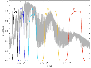
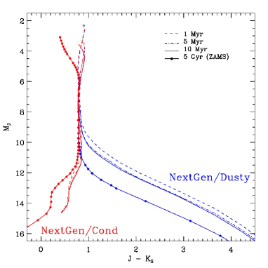
Figure 9: Upper panel: The $ZYJHK_{S}$ VISTA transmission bands. An example of a normalized NextGen spectrum (Hauschildt et al., 1999) with $T_{\rm eff}=2500$ K is over-plotted. Lower panel: Theoretical $M_{J}$ vs. $J-K_{S}$ diagram. The isochrones, shifted to the distance of 10 pc (i.e., absolute magnitudes), are in the VISTA photometric system. Different curve-styles correspond to different ages, as indicated in the legend. We plot in blue the isochrones computed using the NextGen/AMES-Dusty atmospheric models, and in red those computed using the NextGen/AMES-Cond models.

[x]cc—ccccc—ccccc Theoretical isochrones from Baraffe et al. (1998) and Chabrier et al. (2000) converted into the VISTA photometric system.
Mass T_eff $Z$ $Y$ $J$ $H$ $K_{S}$ $Z$ $Y$ $J$ $H$ $K_{S}$
(M_⊙) (K)
Mass T_eff $Z$ $Y$ $J$ $H$ $K_{S}$ $Z$ $Y$ $J$ $H$ $K_{S}$
(M_⊙) (K)
Continued on Next Page… NextGen/AMES-Dusty                                                              NextGen/AMES-Cond
1 Myrs
0.002 1300 20.899 18.949 16.523 13.923 11.824 15.192 13.621 12.496 12.326 11.875
0.002 1400 19.306 17.576 15.410 13.066 11.211 14.251 13.354 12.133 11.904 11.470
0.003 1500 17.958 16.376 14.336 12.237 10.691 13.900 13.042 11.777 11.516 11.055
0.003 1600 16.643 15.123 13.181 11.525 10.300 13.945 12.610 11.426 11.147 10.646
0.004 1700 15.110 13.702 12.031 10.881 9.949 13.754 12.172 11.105 10.812 10.278
0.004 1800 14.359 12.961 11.422 10.511 9.710 13.320 11.773 10.788 10.490 9.941
0.005 1900 13.659 12.310 10.920 10.173 9.463 12.877 11.365 10.482 10.179 9.629
0.006 2000 12.951 11.666 10.427 9.813 9.184 12.420 11.142 10.147 9.837 9.302
0.007 2100 12.354 11.129 10.006 9.475 8.904 11.928 10.960 9.818 9.497 8.984
0.009 2200 11.794 10.636 9.614 9.143 8.623 11.459 10.588 9.531 9.165 8.677
0.011 2300 11.330 10.254 9.319 8.877 8.393 11.091 10.258 9.274 8.904 8.440
0.014 2400 10.816 9.826 8.966 8.541 8.085 10.646 9.867 8.951 8.573 8.128
0.018 2500 10.467 9.568 8.768 8.347 7.913 10.329 9.603 8.753 8.367 7.945
0.024 2600 10.001 9.187 8.436 8.012 7.596 9.893 9.215 8.417 8.025 7.623
0.030 2700 9.386 8.649 7.936 7.507 7.109 9.319 8.691 7.935 7.524 7.129
0.041 2800 8.725 8.050 7.366 6.932 6.552 8.665 8.079 7.359 6.939 6.564
0.062 2900 7.850 7.219 6.556 6.117 5.754 7.766 7.216 6.526 6.097 5.743
0.101 3000 6.846 6.264 5.624 5.173 4.834 6.781 6.262 5.597 5.152 4.822
0.142 3100 6.151 5.613 4.991 4.517 4.205 6.113 5.623 4.977 4.505 4.203
0.207 3200 5.591 5.088 4.482 3.971 3.685 5.565 5.099 4.470 3.958 3.683
0.326 3300 5.075 4.603 4.009 3.454 3.190 5.055 4.614 3.998 3.435 3.185
0.465 3400 4.626 4.180 3.595 2.992 2.750 4.608 4.189 3.581 2.960 2.736
0.590 3500 4.286 3.861 3.279 2.627 2.410 4.275 3.869 3.267 2.595 2.396
0.709 3600 4.008 3.603 3.022 2.324 2.134 4.005 3.618 3.017 2.305 2.126
0.843 3700 3.752 3.369 2.792 2.064 1.887 3.744 3.380 2.785 2.045 1.875
0.985 3800 3.526 3.168 2.601 1.858 1.688 3.515 3.178 2.595 1.845 1.678
1.151 3900 3.258 2.927 2.375 1.637 1.471 3.242 2.928 2.364 1.625 1.463
1.214 4000 3.120 2.832 2.278 1.539 1.367 3.089 2.799 2.252 1.532 1.375
5 Myrs
0.002 900 29.734 26.453 22.394 18.219 15.123 17.537 15.510 14.602 14.666 14.177
0.004 1300 21.184 19.234 16.808 14.208 12.109 15.477 13.906 12.781 12.611 12.160
0.005 1400 19.603 17.874 15.707 13.363 11.509 14.549 13.651 12.431 12.202 11.768
0.006 1500 18.271 16.689 14.649 12.550 11.004 14.213 13.355 12.090 11.829 11.368
0.006 1600 16.974 15.454 13.512 11.856 10.630 14.276 12.941 11.757 11.478 10.976
0.007 1700 15.462 14.055 12.383 11.234 10.302 14.106 12.525 11.458 11.165 10.630
0.008 1800 14.730 13.332 11.793 10.881 10.081 13.691 12.144 11.159 10.861 10.311
0.010 1900 13.994 12.645 11.255 10.508 9.798 13.212 11.700 10.817 10.514 9.964
0.012 2000 13.359 12.075 10.836 10.222 9.593 12.828 11.551 10.555 10.246 9.711
0.013 2100 12.827 11.603 10.480 9.948 9.378 12.402 11.433 10.292 9.971 9.458
0.014 2200 12.329 11.172 10.150 9.679 9.159 11.995 11.124 10.066 9.701 9.213
0.016 2300 11.828 10.752 9.817 9.376 8.891 11.589 10.757 9.772 9.402 8.938
0.018 2400 11.312 10.322 9.461 9.037 8.581 11.141 10.362 9.447 9.068 8.624
0.020 2500 10.845 9.946 9.146 8.725 8.291 10.707 9.982 9.131 8.746 8.323
0.025 2600 10.200 9.386 8.634 8.210 7.794 10.092 9.414 8.615 8.224 7.822
0.030 2700 9.630 8.893 8.180 7.751 7.353 9.563 8.935 8.179 7.768 7.373
0.040 2800 9.181 8.506 7.822 7.388 7.008 9.121 8.534 7.815 7.395 7.020
0.053 2900 8.911 8.280 7.617 7.178 6.815 8.827 8.277 7.587 7.158 6.803
0.076 3000 8.423 7.841 7.200 6.750 6.410 8.357 7.839 7.173 6.728 6.399
0.113 3100 7.853 7.314 6.693 6.218 5.907 7.815 7.324 6.678 6.207 5.904
0.177 3200 7.185 6.682 6.076 5.565 5.279 7.159 6.693 6.064 5.552 5.277
0.261 3300 6.599 6.127 5.533 4.978 4.715 6.579 6.138 5.522 4.959 4.709
0.348 3400 6.152 5.706 5.121 4.519 4.276 6.135 5.715 5.107 4.487 4.263
0.456 3500 5.740 5.315 4.733 4.081 3.864 5.729 5.323 4.721 4.049 3.850
0.588 3600 5.342 4.937 4.356 3.658 3.468 5.339 4.952 4.351 3.639 3.460
0.735 3700 5.000 4.617 4.040 3.312 3.135 4.991 4.627 4.033 3.293 3.123
0.879 3800 4.727 4.370 3.803 3.059 2.889 4.717 4.379 3.797 3.046 2.880
1.006 3900 4.481 4.150 3.598 2.860 2.694 4.465 4.151 3.587 2.848 2.686
1.070 4000 4.313 4.025 3.471 2.732 2.560 4.282 3.992 3.444 2.725 2.568
10 Myrs
0.003 900 29.799 26.519 22.460 18.285 15.189 17.603 15.576 14.668 14.732 14.243
0.006 1300 21.280 19.330 16.904 14.304 12.205 15.573 14.002 12.877 12.707 12.256
0.007 1400 19.718 17.988 15.822 13.478 11.623 14.663 13.766 12.545 12.317 11.882
0.008 1500 18.392 16.810 14.770 12.671 11.125 14.334 13.476 12.211 11.950 11.489
0.010 1600 17.006 15.486 13.544 11.888 10.663 14.308 12.973 11.789 11.510 11.008
0.011 1700 15.501 14.094 12.422 11.273 10.341 14.145 12.564 11.497 11.203 10.669
0.012 1800 14.807 13.408 11.870 10.958 10.157 13.767 12.221 11.236 10.937 10.388
0.013 1900 14.121 12.772 11.382 10.635 9.925 13.338 11.827 10.944 10.641 10.091
0.014 2000 13.452 12.168 10.929 10.315 9.686 12.921 11.644 10.649 10.339 9.804
0.014 2100 12.914 11.689 10.566 10.035 9.465 12.489 11.520 10.379 10.057 9.544
0.016 2200 12.391 11.234 10.212 9.740 9.220 12.057 11.186 10.128 9.762 9.274
0.017 2300 11.856 10.780 9.845 9.403 8.919 11.617 10.784 9.800 9.430 8.966
0.019 2400 11.367 10.377 9.517 9.092 8.636 11.197 10.418 9.502 9.124 8.680
0.021 2500 10.926 10.027 9.227 8.806 8.372 10.788 10.062 9.212 8.826 8.404
0.026 2600 10.536 9.722 8.971 8.547 8.131 10.428 9.750 8.952 8.560 8.158
0.034 2700 10.212 9.475 8.762 8.333 7.935 10.145 9.517 8.761 8.350 7.955
0.045 2800 9.906 9.230 8.547 8.113 7.733 9.845 9.259 8.540 8.120 7.745
0.059 2900 9.514 8.884 8.220 7.782 7.418 9.430 8.880 8.190 7.761 7.407
0.081 3000 8.994 8.412 7.771 7.321 6.981 8.928 8.410 7.744 7.299 6.970
0.105 3100 8.514 7.976 7.354 6.880 6.568 8.476 7.986 7.340 6.868 6.566
0.160 3200 7.875 7.372 6.766 6.255 5.969 7.849 7.383 6.754 6.242 5.967
0.247 3300 7.207 6.735 6.141 5.586 5.323 7.187 6.746 6.130 5.567 5.317
0.354 3400 6.649 6.203 5.618 5.015 4.773 6.631 6.212 5.603 4.983 4.759
0.447 3500 6.279 5.854 5.272 4.620 4.403 6.267 5.862 5.260 4.588 4.389
0.549 3600 5.931 5.526 4.945 4.247 4.056 5.928 5.541 4.940 4.227 4.049
0.674 3700 5.603 5.219 4.643 3.915 3.738 5.594 5.230 4.636 3.896 3.726
0.806 3800 5.292 4.934 4.367 3.623 3.454 5.281 4.943 4.361 3.610 3.444
0.916 3900 5.039 4.708 4.157 3.418 3.253 5.023 4.710 4.145 3.406 3.244
1.000 4000 4.851 4.563 4.009 3.270 3.098 4.820 4.529 3.982 3.263 3.106
50 Myrs
0.008 1000 26.796 24.021 20.576 16.967 14.265 17.196 15.415 14.245 14.536 14.312
0.010 1100 24.515 22.092 19.076 15.874 13.421 16.609 14.773 13.612 13.853 13.497
0.011 1300 21.467 19.485 17.010 14.339 12.215 15.558 13.902 12.789 12.933 12.577
0.012 1500 18.600 17.008 14.980 12.808 11.207 14.785 13.215 12.105 12.125 11.875
0.013 1600 17.366 15.899 13.973 12.121 10.831 14.459 12.909 11.803 11.746 11.511
0.014 1700 15.810 14.427 12.659 11.367 10.459 14.095 12.577 11.527 11.409 11.161
0.015 1800 14.695 13.383 11.806 10.894 10.227 13.739 12.279 11.267 11.097 10.816
0.023 1900 14.656 13.365 11.850 10.998 10.377 13.662 12.228 11.289 11.077 10.753
0.025 2000 14.150 12.897 11.498 10.777 10.233 13.329 12.064 11.072 10.821 10.460
0.028 2100 13.499 12.336 11.108 10.512 10.033 12.973 11.987 10.867 10.582 10.200
0.030 2200 13.077 11.980 10.858 10.317 9.870 12.644 11.814 10.692 10.366 9.971
0.034 2300 12.666 11.640 10.613 10.106 9.680 12.323 11.565 10.494 10.140 9.745
0.041 2500 11.875 11.011 10.148 9.686 9.302 11.688 11.061 10.108 9.712 9.335
0.047 2600 11.496 10.713 9.913 9.455 9.087 11.358 10.781 9.889 9.475 9.111
0.054 2700 11.138 10.431 9.682 9.222 8.866 11.036 10.501 9.668 9.238 8.885
0.064 2800 10.739 10.101 9.396 8.933 8.589 10.670 10.171 9.390 8.947 8.607
0.078 2900 10.332 9.752 9.082 8.614 8.282 10.278 9.810 9.076 8.622 8.294
0.094 3000 9.988 9.457 8.818 8.343 8.025 9.945 9.503 8.811 8.347 8.031
0.112 3100 9.661 9.172 8.558 8.078 7.773 9.641 9.221 8.566 8.089 7.780
0.146 3200 9.213 8.763 8.171 7.681 7.381 9.185 8.787 8.162 7.676 7.381
0.198 3300 8.675 8.252 7.681 7.182 6.903 8.662 8.281 7.685 7.189 6.907
0.287 3400 8.099 7.706 7.154 6.641 6.366 8.080 7.715 7.145 6.633 6.363
0.399 3500 7.548 7.179 6.641 6.113 5.849 7.532 7.182 6.634 6.104 5.844
0.517 3600 7.064 6.716 6.193 5.649 5.393 7.049 6.718 6.184 5.636 5.386
0.588 3700 6.743 6.414 5.903 5.343 5.100 6.732 6.419 5.896 5.331 5.091
0.633 3800 6.503 6.192 5.692 5.119 4.885 6.490 6.192 5.679 5.095 4.870
0.669 3900 6.271 5.973 5.481 4.887 4.674 6.259 5.975 5.470 4.866 4.659
0.703 4000 6.059 5.777 5.291 4.685 4.489 6.046 5.775 5.275 4.653 4.466
100 Myrs
0.010 900 29.315 26.071 22.068 18.154 15.116 17.558 15.865 14.757 15.040 15.076
0.010 1000 26.709 23.933 20.489 16.879 14.178 17.109 15.328 14.158 14.449 14.225
0.011 1100 24.561 22.138 19.122 15.920 13.467 16.655 14.820 13.658 13.900 13.543
0.012 1300 21.506 19.523 17.049 14.377 12.253 15.596 13.940 12.827 12.971 12.615
0.021 1500 18.931 17.339 15.311 13.139 11.537 15.116 13.546 12.436 12.456 12.206
0.024 1600 17.742 16.274 14.349 12.497 11.207 14.835 13.285 12.179 12.122 11.887
0.026 1700 16.230 14.847 13.079 11.787 10.880 14.515 12.998 11.948 11.829 11.581
0.028 1800 15.158 13.847 12.269 11.358 10.691 14.203 12.743 11.731 11.561 11.280
0.031 1900 14.897 13.605 12.091 11.238 10.617 13.903 12.468 11.530 11.317 10.994
0.033 2000 14.391 13.138 11.738 11.018 10.474 13.570 12.305 11.313 11.062 10.701
0.036 2100 13.740 12.577 11.349 10.753 10.274 13.214 12.228 11.108 10.823 10.441
0.039 2200 13.319 12.221 11.099 10.558 10.111 12.886 12.056 10.934 10.608 10.212
0.043 2300 12.918 11.892 10.865 10.358 9.932 12.575 11.817 10.745 10.392 9.997
0.051 2500 12.135 11.271 10.408 9.946 9.562 11.948 11.321 10.368 9.972 9.595
0.057 2600 11.773 10.990 10.190 9.732 9.364 11.635 11.058 10.167 9.753 9.388
0.064 2700 11.425 10.717 9.968 9.508 9.152 11.323 10.787 9.954 9.524 9.171
0.073 2800 11.063 10.425 9.721 9.257 8.914 10.995 10.495 9.715 9.271 8.932
0.087 2900 10.698 10.118 9.448 8.979 8.648 10.644 10.175 9.442 8.988 8.660
0.104 3000 10.375 9.844 9.204 8.730 8.411 10.332 9.890 9.198 8.734 8.418
0.123 3100 10.040 9.551 8.937 8.457 8.152 10.020 9.600 8.945 8.468 8.159
0.150 3200 9.664 9.214 8.623 8.133 7.833 9.636 9.238 8.614 8.128 7.832
0.201 3300 9.155 8.733 8.162 7.662 7.384 9.142 8.761 8.166 7.669 7.387
0.277 3400 8.611 8.219 7.666 7.153 6.879 8.592 8.228 7.658 7.146 6.875
0.377 3500 8.068 7.698 7.161 6.632 6.369 8.051 7.701 7.153 6.624 6.364
0.461 3600 7.595 7.247 6.724 6.180 5.924 7.580 7.248 6.714 6.167 5.916
0.514 3700 7.248 6.919 6.408 5.848 5.605 7.237 6.924 6.401 5.836 5.596
0.548 3800 6.999 6.688 6.188 5.615 5.381 6.986 6.688 6.175 5.591 5.366
0.579 3900 6.772 6.475 5.982 5.388 5.175 6.760 6.476 5.971 5.368 5.160
0.603 4000 6.580 6.298 5.813 5.207 5.010 6.567 6.297 5.796 5.174 4.988
5 Gyrs (ZAMS)
0.050 900 30.203 26.959 22.956 19.042 16.004 18.446 16.753 15.645 15.928 15.964
0.055 1000 27.670 24.895 21.451 17.841 15.140 18.071 16.289 15.119 15.410 15.187
0.060 1100 25.589 23.166 20.150 16.948 14.494 17.683 15.847 14.685 14.927 14.571
0.064 1300 22.585 20.603 18.128 15.457 13.333 16.676 15.020 13.907 14.051 13.695
0.068 1500 19.766 18.175 16.146 13.975 12.373 15.951 14.381 13.272 13.292 13.042
0.070 1600 18.561 17.094 15.169 13.317 12.026 15.654 14.105 12.999 12.941 12.706
0.071 1700 17.018 15.636 13.867 12.576 11.668 15.303 13.786 12.736 12.617 12.369
0.073 1800 15.917 14.605 13.028 12.116 11.449 14.961 13.501 12.489 12.319 12.038
0.074 1900 15.631 14.339 12.825 11.972 11.351 14.637 13.202 12.264 12.051 11.728
0.075 2000 15.119 13.866 12.466 11.746 11.202 14.298 13.033 12.041 11.790 11.429
0.077 2100 14.429 13.266 12.038 11.441 10.963 13.903 12.917 11.797 11.512 11.130
0.078 2200 13.970 12.872 11.751 11.210 10.762 13.537 12.707 11.585 11.259 10.864
0.080 2300 13.551 12.525 11.498 10.991 10.565 13.208 12.450 11.379 11.025 10.630
0.086 2500 12.709 11.845 10.982 10.520 10.137 12.522 11.895 10.942 10.546 10.169
0.089 2600 12.350 11.567 10.766 10.309 9.941 12.211 11.635 10.743 10.329 9.964
0.095 2700 11.989 11.281 10.532 10.072 9.716 11.887 11.351 10.518 10.088 9.735
0.101 2800 11.637 11.000 10.295 9.831 9.488 11.569 11.069 10.289 9.846 9.506
0.108 2900 11.307 10.727 10.058 9.589 9.257 11.253 10.785 10.052 9.597 9.269
0.122 3000 10.914 10.382 9.743 9.268 8.950 10.870 10.428 9.736 9.272 8.956
0.139 3100 10.506 10.017 9.403 8.923 8.618 10.486 10.066 9.411 8.934 8.625
0.165 3200 10.075 9.625 9.034 8.544 8.244 10.047 9.649 9.025 8.539 8.243
0.205 3300 9.542 9.120 8.549 8.049 7.771 9.529 9.148 8.553 8.056 7.774
0.270 3400 8.937 8.544 7.992 7.479 7.205 8.918 8.553 7.983 7.471 7.201
0.377 3500 8.215 7.845 7.308 6.779 6.516 8.198 7.848 7.300 6.771 6.511
0.463 3600 7.673 7.325 6.802 6.258 6.002 7.658 7.327 6.793 6.245 5.995
0.523 3700 7.274 6.944 6.434 5.874 5.630 7.263 6.949 6.427 5.861 5.622
0.568 3800 6.981 6.670 6.170 5.597 5.363 6.968 6.670 6.157 5.573 5.348
0.602 3900 6.731 6.434 5.941 5.347 5.134 6.719 6.436 5.930 5.327 5.120
0.631 4000 6.517 6.234 5.749 5.143 4.946 6.503 6.233 5.732 5.110 4.924

[x]cccccccccccccc VISTA and Spitzer observed magnitudes for the YSO candidates in L1630 N. When the photometric errors are not reported, the corresponding magnitude is an upper limit to the actual brightness of the object. The “–” symbol indicates that the object has not been detected in the given VISTA pass-band. The Lada classes marked with “?” are uncertain because the corresponding K_S magnitude is uncertain (i.e. photometric contamination, large photmetric errors, object truncated or partially saturated, etc.). Column 3 specifies whether the object has been previously identified by Flaherty & Muzerolle (2008) (F08) and/or Fang et al. (2009) (FA09) .
ID Name/Position Previous Lada $Z$ $Y$ $J$ $H$ $K_{S}$ IRAC IRAC IRAC IRAC MIPS
(VISTAomsJ) Identification Class 3.6$\mu$m 4.5$\mu$m 5.8$\mu$m 8$\mu$m 24$\mu$m
ID Name/Position Previous Lada $Z$ $Y$ $J$ $H$ $K_{S}$ IRAC IRAC IRAC IRAC MIPS
(VISTAomsJ) Identification Class 3.6$\mu$m 4.5$\mu$m 5.8$\mu$m 8$\mu$m 24$\mu$m

Continued on Next Page…

1 054803.999+000341.11 III? 10.635 10.153 8.723 8.467 7.167 6.526 $\pm$ 0.002 6.559 $\pm$ 0.001 6.353 $\pm$ 0.001 6.178 $\pm$ 0.001 5.251 $\pm$ 0.009
2 054713.848+000016.92 F08/FA09 II? 11.748 11.129 10.129 9.310 8.728 8.233 $\pm$ 0.003 7.824 $\pm$ 0.003 7.599 $\pm$ 0.001 7.022 $\pm$ 0.001 4.531 $\pm$ 0.014
3 054619.061+000329.56 F08/FA09 Flat 12.530 11.655 10.414 11.383 $\pm$ 0.001 10.029 $\pm$ 0.001 6.542 $\pm$ 0.002 6.005 $\pm$ 0.002 5.597 $\pm$ 0.003 4.937 $\pm$ 0.002 2.231 $\pm$ 0.013
4 054811.880-002157.46 III? 11.994 11.216 10.427 9.418 9.016 8.981 $\pm$ 0.005 8.972 $\pm$ 0.002 8.841 $\pm$ 0.003 8.758 $\pm$ 0.004 8.593 $\pm$ 0.145
5 054619.470-000519.97 F08/FA09 II? 11.986 – 10.602 9.668 9.127 7.960 $\pm$ 0.003 7.497 $\pm$ 0.002 7.151 $\pm$ 0.002 6.052 $\pm$ 0.003 3.002 $\pm$ 0.010
6 054705.993+003208.41 F08/FA09 II? 13.361 $\pm$ 0.001 12.570 10.705 10.013 9.275 8.095 $\pm$ 0.003 7.578 $\pm$ 0.003 7.249 $\pm$ 0.001 6.527 $\pm$ 0.001 3.101 $\pm$ 0.009
7 054604.671+000458.01 F08/FA09 II? 11.511 11.854 10.926 9.954 9.301 8.296 $\pm$ 0.003 7.887 $\pm$ 0.004 7.472 $\pm$ 0.001 6.692 $\pm$ 0.001 3.796 $\pm$ 0.015
8 054618.893-000538.11 F08/FA09 II? 12.560 11.911 11.129 10.291 9.875 8.945 $\pm$ 0.005 8.654 $\pm$ 0.001 8.183 $\pm$ 0.002 7.568 $\pm$ 0.002 5.730 $\pm$ 0.013
9 054707.262+001932.16 F08/FA09 Flat 12.181 11.280 11.146 $\pm$ 0.001 11.039 $\pm$ 0.001 10.135 $\pm$ 0.001 7.400 $\pm$ 0.002 6.883 $\pm$ 0.002 6.429 $\pm$ 0.001 5.582 $\pm$ 0.004 3.292 $\pm$ 0.016
10 054658.138+000538.33 F08/FA09 II? 12.960 12.162 11.210 10.256 9.847 9.395 $\pm$ 0.005 9.204 $\pm$ 0.001 8.943 $\pm$ 0.007 8.464 $\pm$ 0.022 5.066 $\pm$ 0.012
11 054714.110+000907.34 F08 I 12.548 $\pm$ 0.001 12.254 $\pm$ 0.001 11.280 $\pm$ 0.001 11.142 $\pm$ 0.001 10.877 $\pm$ 0.001 6.685 $\pm$ 0.001 5.703 $\pm$ 0.001 5.074 $\pm$ 0.002 3.974 $\pm$ 0.001 1.057 $\pm$ 0.007
12 054706.960+000047.66 F08/FA09 II? 12.420 11.836 11.316 10.602 10.353 9.818 $\pm$ 0.001 9.582 $\pm$ 0.001 9.219 $\pm$ 0.003 8.170 $\pm$ 0.003 4.878 $\pm$ 0.014
13 054609.261+001332.70 F08/FA09 II? 12.649 11.850 11.332 10.134 9.765 8.947 $\pm$ 0.004 8.603 $\pm$ 0.002 8.083 $\pm$ 0.001 7.468 $\pm$ 0.002 4.358 $\pm$ 0.012
14 054607.884-001156.83 F08/FA09 III? 12.387 $\pm$ 0.001 12.101 $\pm$ 0.001 11.352 $\pm$ 0.001 8.356 8.195 8.106 $\pm$ 0.003 7.974 $\pm$ 0.003 7.720 $\pm$ 0.002 7.293 $\pm$ 0.001 5.116 $\pm$ 0.006
15 054637.061+000121.86 F08/FA09 II? 13.273 $\pm$ 0.001 12.312 11.409 11.147 $\pm$ 0.001 9.621 8.226 $\pm$ 0.003 7.791 $\pm$ 0.003 7.426 $\pm$ 0.003 6.700 $\pm$ 0.007 3.126 $\pm$ 0.006
16 054622.436-000852.58 F08/FA09 II? 12.574 12.150 11.414 11.333 $\pm$ 0.001 10.281 9.542 $\pm$ 0.001 9.364 $\pm$ 0.001 9.177 $\pm$ 0.003 8.491 $\pm$ 0.002 4.797 $\pm$ 0.011
17 054611.869+003225.91 F08/FA09 II 12.656 $\pm$ 0.001 12.424 $\pm$ 0.001 11.457 $\pm$ 0.001 11.444 $\pm$ 0.001 10.486 $\pm$ 0.001 8.680 $\pm$ 0.004 8.580 $\pm$ 0.002 8.382 $\pm$ 0.002 8.142 $\pm$ 0.002 4.348 $\pm$ 0.015
18 054545.588+002556.96 II 15.487 $\pm$ 0.002 13.431 $\pm$ 0.001 11.537 $\pm$ 0.001 11.628 $\pm$ 0.001 10.952 $\pm$ 0.001 6.687 $\pm$ 0.002 6.539 $\pm$ 0.002 6.238 $\pm$ 0.001 6.091 $\pm$ 0.004 5.363 $\pm$ 0.014
19 054645.813+001702.51 II 12.819 $\pm$ 0.001 12.552 $\pm$ 0.001 11.543 $\pm$ 0.001 11.320 $\pm$ 0.001 10.411 $\pm$ 0.001 8.759 $\pm$ 0.004 8.376 $\pm$ 0.004 7.994 $\pm$ 0.002 7.385 $\pm$ 0.002 4.459 $\pm$ 0.017
20 054650.215+000439.61 II? 12.879 12.386 11.550 10.745 10.173 9.437 $\pm$ 0.002 8.810 $\pm$ 0.001 8.398 $\pm$ 0.009 7.423 $\pm$ 0.024 3.763 $\pm$ 0.016
21 054631.053+002533.74 F08 Flat 13.142 12.503 11.559 11.271 $\pm$ 0.001 10.343 $\pm$ 0.001 8.445 $\pm$ 0.004 7.887 $\pm$ 0.003 7.389 $\pm$ 0.002 6.441 $\pm$ 0.001 3.428 $\pm$ 0.010
22 054644.083+001803.17 F08/FA09 II 13.085 $\pm$ 0.001 12.574 $\pm$ 0.001 11.587 11.323 $\pm$ 0.001 10.517 $\pm$ 0.001 9.433 $\pm$ 0.005 9.130 $\pm$ 0.002 8.717 $\pm$ 0.002 8.049 $\pm$ 0.003 5.857 $\pm$ 0.021
23 054557.384+002022.20 F08/FA09 II? 13.172 $\pm$ 0.001 12.790 $\pm$ 0.001 11.837 11.535 $\pm$ 0.001 10.509 9.291 $\pm$ 0.001 9.009 $\pm$ 0.002 8.807 $\pm$ 0.003 8.099 $\pm$ 0.002 5.007 $\pm$ 0.014
24 054541.948-001205.26 F08/FA09 II 13.035 $\pm$ 0.001 12.845 $\pm$ 0.001 11.986 $\pm$ 0.001 11.577 $\pm$ 0.001 11.071 $\pm$ 0.002 10.862 $\pm$ 0.002 10.947 $\pm$ 0.003 10.741 $\pm$ 0.011 10.667 $\pm$ 0.011 6.498 $\pm$ 0.040
25 054634.539+000643.49 F08/FA09 II? 14.277 $\pm$ 0.001 13.273 $\pm$ 0.001 12.007 $\pm$ 0.001 11.238 $\pm$ 0.001 9.559 8.736 $\pm$ 0.004 8.266 $\pm$ 0.004 7.901 $\pm$ 0.003 7.230 $\pm$ 0.009 4.990 $\pm$ 0.009
26 054600.178+000307.09 F08/FA09 II? 13.300 12.687 12.015 11.309 10.957 10.425 $\pm$ 0.002 10.110 $\pm$ 0.002 9.725 $\pm$ 0.004 8.932 $\pm$ 0.003 5.652 $\pm$ 0.016
27 054645.040+000533.90 FA09 II? 13.912 $\pm$ 0.001 12.812 12.025 $\pm$ 0.001 10.753 10.218 9.427 $\pm$ 0.004 8.972 $\pm$ 0.004 8.530 $\pm$ 0.006 7.707 $\pm$ 0.017 4.372 $\pm$ 0.028
28 054646.871+000907.67 F08/FA09 II? 13.457 $\pm$ 0.001 13.171 $\pm$ 0.001 12.026 $\pm$ 0.001 11.116 10.224 9.614 $\pm$ 0.002 9.073 $\pm$ 0.001 8.713 $\pm$ 0.011 7.708 $\pm$ 0.025 4.351 $\pm$ 0.014
29 054618.296+000657.82 F08/FA09 II? 13.710 $\pm$ 0.001 12.950 12.091 $\pm$ 0.001 11.511 $\pm$ 0.001 10.524 9.534 $\pm$ 0.002 9.085 $\pm$ 0.001 8.604 $\pm$ 0.004 7.690 $\pm$ 0.008 4.916 $\pm$ 0.018
30 054556.316+000708.58 F08/FA09 II 13.295 $\pm$ 0.001 12.691 12.140 $\pm$ 0.001 11.410 11.093 $\pm$ 0.002 10.168 $\pm$ 0.002 9.921 $\pm$ 0.002 9.642 $\pm$ 0.004 9.241 $\pm$ 0.004 5.398 $\pm$ 0.013
31 054626.649+003107.43 F08/FA09 II? 13.921 $\pm$ 0.001 13.391 $\pm$ 0.001 12.182 $\pm$ 0.001 11.232 10.463 9.545 $\pm$ 0.001 9.163 $\pm$ 0.002 8.819 $\pm$ 0.002 8.142 $\pm$ 0.002 5.883 $\pm$ 0.014
32 054647.287+000407.10 II? 14.186 $\pm$ 0.001 13.930 $\pm$ 0.001 12.229 $\pm$ 0.001 10.482 9.556 8.664 $\pm$ 0.004 8.176 $\pm$ 0.004 7.773 $\pm$ 0.004 7.061 $\pm$ 0.014 4.180 $\pm$ 0.010
33 054544.374+002258.30 F08/FA09 II? 13.566 $\pm$ 0.001 12.965 $\pm$ 0.001 12.242 $\pm$ 0.001 11.157 10.615 9.387 $\pm$ 0.001 8.943 $\pm$ 0.001 8.667 $\pm$ 0.003 8.006 $\pm$ 0.002 5.265 $\pm$ 0.011
34 054633.285+000251.94 F08/FA09 II? 14.334 $\pm$ 0.001 13.694 $\pm$ 0.001 12.247 $\pm$ 0.001 10.980 10.059 8.838 $\pm$ 0.004 8.374 $\pm$ 0.001 7.958 $\pm$ 0.003 7.251 $\pm$ 0.004 4.785 $\pm$ 0.017
35 054553.544+003308.75 F08/FA09 II 13.727 $\pm$ 0.001 13.074 $\pm$ 0.001 12.280 $\pm$ 0.001 11.666 $\pm$ 0.001 10.963 $\pm$ 0.001 10.200 $\pm$ 0.001 9.857 $\pm$ 0.002 9.426 $\pm$ 0.003 8.686 $\pm$ 0.003 6.002 $\pm$ 0.020
36 054703.977+001114.32 F08/FA09 II 13.630 $\pm$ 0.001 13.158 $\pm$ 0.001 12.304 $\pm$ 0.001 11.742 $\pm$ 0.001 10.968 $\pm$ 0.001 10.074 $\pm$ 0.002 9.649 $\pm$ 0.002 9.261 $\pm$ 0.004 8.349 $\pm$ 0.002 5.360 $\pm$ 0.012
37 054618.012+001212.28 II? 14.043 $\pm$ 0.001 13.944 $\pm$ 0.001 12.340 $\pm$ 0.001 11.704 10.562 9.714 $\pm$ 0.001 9.289 $\pm$ 0.002 9.019 $\pm$ 0.003 8.622 $\pm$ 0.003 6.363 $\pm$ 0.016
38 054630.057+001209.61 F08/FA09 II 14.146 $\pm$ 0.001 13.310 $\pm$ 0.001 12.364 $\pm$ 0.001 11.222 10.834 $\pm$ 0.001 9.841 $\pm$ 0.002 9.521 $\pm$ 0.002 9.247 $\pm$ 0.004 8.384 $\pm$ 0.002 5.434 $\pm$ 0.015
39 054620.872+000809.35 F08/FA09 II? 14.295 $\pm$ 0.001 13.488 $\pm$ 0.001 12.405 $\pm$ 0.001 11.619 $\pm$ 0.001 10.489 9.922 $\pm$ 0.001 9.501 $\pm$ 0.002 9.016 $\pm$ 0.003 8.081 $\pm$ 0.004 4.905 $\pm$ 0.016
40 054710.891+003205.96 F08/FA09 II 13.856 $\pm$ 0.001 13.238 $\pm$ 0.001 12.524 $\pm$ 0.002 11.504 11.083 $\pm$ 0.002 10.404 $\pm$ 0.002 10.035 $\pm$ 0.002 9.627 $\pm$ 0.003 9.032 $\pm$ 0.004 6.768 $\pm$ 0.016
41 054652.409+002001.64 F08/FA09 II? 14.208 $\pm$ 0.001 13.474 $\pm$ 0.001 12.553 $\pm$ 0.002 11.451 10.874 9.739 $\pm$ 0.001 9.314 $\pm$ 0.002 8.962 $\pm$ 0.004 8.058 $\pm$ 0.014 4.637 $\pm$ 0.011
42 054604.774-001416.48 I 17.138 $\pm$ 0.005 15.148 $\pm$ 0.002 12.664 $\pm$ 0.002 11.264 $\pm$ 0.001 10.175 $\pm$ 0.001 7.222 $\pm$ 0.002 6.276 $\pm$ 0.002 5.404 $\pm$ 0.002 4.419 $\pm$ 0.002 0.638 $\pm$ 0.007
43 054634.898+000420.75 F08/FA09 II 14.562 $\pm$ 0.001 13.619 $\pm$ 0.001 12.752 $\pm$ 0.002 11.653 11.208 $\pm$ 0.002 10.753 $\pm$ 0.003 10.605 $\pm$ 0.003 10.248 $\pm$ 0.021 9.884 $\pm$ 0.052 6.904 $\pm$ 0.041
44 054647.404+001259.26 II 14.784 $\pm$ 0.002 13.934 $\pm$ 0.001 12.767 $\pm$ 0.002 11.661 11.015 $\pm$ 0.002 10.169 $\pm$ 0.001 9.742 $\pm$ 0.002 9.298 $\pm$ 0.004 8.728 $\pm$ 0.003 6.644 $\pm$ 0.023
45 054726.329+001848.35 II 14.844 $\pm$ 0.002 13.812 $\pm$ 0.001 12.771 $\pm$ 0.002 11.705 11.169 $\pm$ 0.002 10.563 $\pm$ 0.002 10.345 $\pm$ 0.002 10.078 $\pm$ 0.007 9.534 $\pm$ 0.018 6.990 $\pm$ 0.048
46 054703.314+002323.21 II? 15.603 $\pm$ 0.002 14.248 $\pm$ 0.002 12.774 $\pm$ 0.002 11.198 10.461 9.812 $\pm$ 0.002 9.553 $\pm$ 0.003 9.214 $\pm$ 0.004 8.680 $\pm$ 0.007 6.651 $\pm$ 0.034
47 054553.115-001324.85 F08/FA09 II 13.879 $\pm$ 0.001 13.429 $\pm$ 0.001 12.791 $\pm$ 0.002 12.090 $\pm$ 0.002 11.785 $\pm$ 0.002 11.362 $\pm$ 0.002 11.280 $\pm$ 0.003 11.214 $\pm$ 0.009 10.942 $\pm$ 0.015 6.456 $\pm$ 0.025
48 054643.843+001532.29 F08/FA09 II 14.237 $\pm$ 0.001 13.670 $\pm$ 0.001 12.811 $\pm$ 0.002 12.016 $\pm$ 0.002 11.361 $\pm$ 0.002 10.350 $\pm$ 0.001 10.393 $\pm$ 0.002 9.667 $\pm$ 0.004 9.357 $\pm$ 0.004 6.923 $\pm$ 0.028
49 054616.747+000713.37 FA09 II 15.174 $\pm$ 0.002 13.946 $\pm$ 0.001 12.815 $\pm$ 0.002 11.816 $\pm$ 0.001 11.122 $\pm$ 0.002 10.537 $\pm$ 0.002 10.286 $\pm$ 0.002 10.020 $\pm$ 0.007 9.597 $\pm$ 0.017 6.905 $\pm$ 0.035
50 054628.885+001331.15 FA09 II? 15.418 $\pm$ 0.002 14.371 $\pm$ 0.002 12.859 $\pm$ 0.002 11.392 10.142 9.090 $\pm$ 0.001 8.594 $\pm$ 0.002 8.154 $\pm$ 0.002 7.271 $\pm$ 0.001 4.343 $\pm$ 0.010
51 054716.584-000056.38 F08/FA09 II 14.297 $\pm$ 0.001 13.619 $\pm$ 0.001 12.874 $\pm$ 0.002 12.224 $\pm$ 0.002 11.709 $\pm$ 0.002 11.209 $\pm$ 0.002 10.842 $\pm$ 0.003 10.489 $\pm$ 0.006 9.827 $\pm$ 0.008 7.547 $\pm$ 0.039
52 054653.579+000005.80 Flat? 15.329 $\pm$ 0.002 13.957 $\pm$ 0.001 12.885 $\pm$ 0.002 11.075 10.282 8.791 $\pm$ 0.004 8.182 $\pm$ 0.004 7.626 $\pm$ 0.002 6.630 $\pm$ 0.002 3.318 $\pm$ 0.011
53 054640.768+002722.54 F08/FA09 II 14.642 $\pm$ 0.002 14.010 $\pm$ 0.001 12.893 $\pm$ 0.002 12.245 $\pm$ 0.002 11.400 $\pm$ 0.002 10.274 $\pm$ 0.001 9.866 $\pm$ 0.002 9.524 $\pm$ 0.003 8.877 $\pm$ 0.003 6.366 $\pm$ 0.021
54 054631.566+000640.00 II 15.063 $\pm$ 0.002 14.194 $\pm$ 0.001 12.920 $\pm$ 0.002 11.636 10.995 $\pm$ 0.002 10.260 $\pm$ 0.002 9.899 $\pm$ 0.002 9.520 $\pm$ 0.008 8.854 $\pm$ 0.021 6.441 $\pm$ 0.026
55 054658.032+001427.85 F08/FA09 II 14.563 $\pm$ 0.001 13.697 $\pm$ 0.001 12.932 $\pm$ 0.002 12.079 $\pm$ 0.002 11.536 $\pm$ 0.002 10.658 $\pm$ 0.002 10.264 $\pm$ 0.002 9.778 $\pm$ 0.006 8.985 $\pm$ 0.016 5.922 $\pm$ 0.016
56 054707.925+002024.68 II 14.955 $\pm$ 0.002 13.982 $\pm$ 0.001 12.941 $\pm$ 0.002 11.719 11.149 $\pm$ 0.002 10.489 $\pm$ 0.003 10.128 $\pm$ 0.003 9.628 $\pm$ 0.009 8.727 $\pm$ 0.017 5.801 $\pm$ 0.021
57 054706.169+002032.50 FA09 II? 15.665 $\pm$ 0.002 14.368 $\pm$ 0.002 12.963 $\pm$ 0.002 11.405 10.627 9.724 $\pm$ 0.003 9.243 $\pm$ 0.002 8.719 $\pm$ 0.010 7.862 $\pm$ 0.022 4.479 $\pm$ 0.012
58 054653.769+000034.06 II 15.027 $\pm$ 0.002 13.983 $\pm$ 0.001 12.980 $\pm$ 0.002 12.050 $\pm$ 0.002 11.457 $\pm$ 0.002 10.687 $\pm$ 0.003 10.356 $\pm$ 0.002 10.001 $\pm$ 0.020 9.293 $\pm$ 0.044 6.020 $\pm$ 0.022
59 054706.984+003155.96 F08/FA09 II 14.896 $\pm$ 0.002 13.915 $\pm$ 0.001 13.016 $\pm$ 0.002 11.791 11.271 $\pm$ 0.002 10.137 $\pm$ 0.002 9.502 $\pm$ 0.001 9.107 $\pm$ 0.003 8.079 $\pm$ 0.002 4.694 $\pm$ 0.009
60 054622.987+000426.47 F08/FA09 II 14.756 $\pm$ 0.002 13.925 $\pm$ 0.001 13.048 $\pm$ 0.002 12.082 $\pm$ 0.002 11.544 $\pm$ 0.002 10.786 $\pm$ 0.002 10.398 $\pm$ 0.002 9.940 $\pm$ 0.008 9.182 $\pm$ 0.018 6.336 $\pm$ 0.021
61 054625.882+000931.93 F08/FA09 II 14.417 $\pm$ 0.001 13.800 $\pm$ 0.001 13.058 $\pm$ 0.002 12.248 $\pm$ 0.002 11.734 $\pm$ 0.002 10.847 $\pm$ 0.002 10.373 $\pm$ 0.002 10.120 $\pm$ 0.007 9.382 $\pm$ 0.019 6.639 $\pm$ 0.019
62 054651.478+001921.32 F08/FA09 II 14.682 $\pm$ 0.002 13.883 $\pm$ 0.001 13.132 $\pm$ 0.002 12.284 $\pm$ 0.002 11.802 $\pm$ 0.002 11.232 $\pm$ 0.003 10.929 $\pm$ 0.002 10.638 $\pm$ 0.016 9.664 $\pm$ 0.021 6.333 $\pm$ 0.019
63 054717.162+001824.55 F08/FA09 II 14.745 $\pm$ 0.002 14.143 $\pm$ 0.001 13.150 $\pm$ 0.002 12.105 $\pm$ 0.002 11.246 $\pm$ 0.002 10.065 $\pm$ 0.002 9.537 $\pm$ 0.002 9.249 $\pm$ 0.017 8.725 $\pm$ 0.066 5.977 $\pm$ 0.021
64 054644.837+001659.81 F08/FA09 II 14.879 $\pm$ 0.002 14.033 $\pm$ 0.001 13.169 $\pm$ 0.002 12.135 $\pm$ 0.002 11.626 $\pm$ 0.002 10.999 $\pm$ 0.003 10.818 $\pm$ 0.003 10.655 $\pm$ 0.011 10.091 $\pm$ 0.021 5.872 $\pm$ 0.016
65 054636.105+000626.86 FA09 Flat 16.765 $\pm$ 0.004 15.373 $\pm$ 0.003 13.169 $\pm$ 0.002 11.270 10.373 $\pm$ 0.001 8.409 $\pm$ 0.004 7.935 $\pm$ 0.003 7.459 $\pm$ 0.003 6.201 $\pm$ 0.005 2.434 $\pm$ 0.009
66 054719.186+001920.64 II 14.882 $\pm$ 0.002 14.052 $\pm$ 0.001 13.178 $\pm$ 0.002 12.239 $\pm$ 0.002 11.694 $\pm$ 0.002 10.770 $\pm$ 0.003 10.374 $\pm$ 0.002 9.846 $\pm$ 0.009 8.711 $\pm$ 0.021 5.247 $\pm$ 0.013
67 054638.324+000548.77 FA09 II 16.080 $\pm$ 0.003 14.922 $\pm$ 0.002 13.251 $\pm$ 0.002 12.237 $\pm$ 0.002 11.114 $\pm$ 0.002 9.891 $\pm$ 0.003 9.276 $\pm$ 0.002 8.861 $\pm$ 0.009 7.940 $\pm$ 0.022 4.702 $\pm$ 0.020
68 054638.401+001511.63 FA09 II 15.078 $\pm$ 0.002 14.156 $\pm$ 0.001 13.273 $\pm$ 0.002 12.515 $\pm$ 0.002 11.983 $\pm$ 0.002 11.342 $\pm$ 0.002 11.074 $\pm$ 0.002 10.817 $\pm$ 0.007 10.284 $\pm$ 0.007 7.402 $\pm$ 0.034
69 054637.537+000800.49 II 15.457 $\pm$ 0.002 14.524 $\pm$ 0.002 13.277 $\pm$ 0.002 11.966 11.268 $\pm$ 0.002 10.540 $\pm$ 0.003 10.135 $\pm$ 0.002 9.881 $\pm$ 0.015 9.319 $\pm$ 0.036 6.735 $\pm$ 0.032
70 054629.584+001057.22 FA09 II 15.502 $\pm$ 0.002 14.373 $\pm$ 0.002 13.303 $\pm$ 0.002 12.343 $\pm$ 0.002 11.718 $\pm$ 0.002 10.829 $\pm$ 0.002 10.435 $\pm$ 0.002 9.934 $\pm$ 0.006 9.232 $\pm$ 0.017 6.522 $\pm$ 0.024
71 054653.723+002631.27 II 15.152 $\pm$ 0.002 14.242 $\pm$ 0.002 13.333 $\pm$ 0.002 12.503 $\pm$ 0.002 12.045 $\pm$ 0.002 11.597 $\pm$ 0.002 11.327 $\pm$ 0.003 11.193 $\pm$ 0.008 10.541 $\pm$ 0.011 8.319 $\pm$ 0.061
72 054645.145+000346.44 FA09 II 15.294 $\pm$ 0.002 14.314 $\pm$ 0.002 13.341 $\pm$ 0.002 12.190 $\pm$ 0.002 11.438 $\pm$ 0.002 10.562 $\pm$ 0.005 10.247 $\pm$ 0.005 10.073 $\pm$ 0.034 9.314 $\pm$ 0.094 6.244 $\pm$ 0.031
73 054610.303-000006.70 FA09 II 15.223 $\pm$ 0.002 14.472 $\pm$ 0.002 13.431 $\pm$ 0.002 12.457 $\pm$ 0.002 11.522 $\pm$ 0.002 10.614 $\pm$ 0.002 10.083 $\pm$ 0.002 9.637 $\pm$ 0.004 8.791 $\pm$ 0.008 5.769 $\pm$ 0.013
74 054654.434+002114.18 II 15.995 $\pm$ 0.003 15.132 $\pm$ 0.002 13.434 $\pm$ 0.002 12.668 $\pm$ 0.002 11.550 $\pm$ 0.002 10.734 $\pm$ 0.002 10.315 $\pm$ 0.002 9.938 $\pm$ 0.004 9.341 $\pm$ 0.012 6.592 $\pm$ 0.027
75 054705.301+002310.10 II? 17.542 $\pm$ 0.006 15.822 $\pm$ 0.003 13.473 $\pm$ 0.002 10.786 9.439 7.978 $\pm$ 0.003 7.424 $\pm$ 0.003 6.954 $\pm$ 0.001 6.430 $\pm$ 0.001 3.302 $\pm$ 0.011
76 054651.850+001938.57 FA09 II 15.637 $\pm$ 0.002 14.608 $\pm$ 0.002 13.510 $\pm$ 0.002 12.452 $\pm$ 0.002 11.817 $\pm$ 0.002 11.127 $\pm$ 0.003 10.782 $\pm$ 0.003 10.371 $\pm$ 0.025 9.416 $\pm$ 0.045 5.739 $\pm$ 0.020
77 054632.714+000851.72 II 15.738 $\pm$ 0.003 14.697 $\pm$ 0.002 13.516 $\pm$ 0.002 12.078 $\pm$ 0.002 11.100 $\pm$ 0.002 9.614 $\pm$ 0.002 9.048 $\pm$ 0.001 8.658 $\pm$ 0.003 8.022 $\pm$ 0.006 5.760 $\pm$ 0.018
78 054727.365+000515.29 II 15.992 $\pm$ 0.003 14.697 $\pm$ 0.002 13.521 $\pm$ 0.002 12.219 $\pm$ 0.002 11.380 $\pm$ 0.002 10.105 $\pm$ 0.002 9.470 $\pm$ 0.001 9.002 $\pm$ 0.003 8.358 $\pm$ 0.002 5.646 $\pm$ 0.013
79 054638.566+002206.02 F08/FA09 II 15.568 $\pm$ 0.002 14.422 $\pm$ 0.002 13.588 $\pm$ 0.003 12.260 $\pm$ 0.002 11.840 $\pm$ 0.002 11.137 $\pm$ 0.002 10.842 $\pm$ 0.002 10.502 $\pm$ 0.007 9.853 $\pm$ 0.006 7.673 $\pm$ 0.045
80 054719.722+000121.86 F08/FA09 II 15.240 $\pm$ 0.002 14.330 $\pm$ 0.002 13.632 $\pm$ 0.003 13.060 $\pm$ 0.003 12.648 $\pm$ 0.003 11.737 $\pm$ 0.003 11.158 $\pm$ 0.002 10.785 $\pm$ 0.007 10.168 $\pm$ 0.007 7.102 $\pm$ 0.028
81 054646.961+000709.05 II? 16.576 $\pm$ 0.004 15.162 $\pm$ 0.002 13.641 $\pm$ 0.003 11.960 10.921 9.561 $\pm$ 0.003 8.925 $\pm$ 0.002 8.352 $\pm$ 0.011 7.554 $\pm$ 0.030 4.721 $\pm$ 0.016
82 054557.929+000248.62 F08/FA09 II 15.161 $\pm$ 0.002 14.216 $\pm$ 0.002 13.659 $\pm$ 0.003 12.762 $\pm$ 0.002 12.282 $\pm$ 0.003 11.373 $\pm$ 0.003 11.134 $\pm$ 0.003 10.887 $\pm$ 0.009 10.412 $\pm$ 0.013 7.806 $\pm$ 0.050
83 054604.579+000038.09 F08/FA09 II 15.432 $\pm$ 0.002 14.190 $\pm$ 0.001 13.665 $\pm$ 0.003 12.320 $\pm$ 0.002 12.016 $\pm$ 0.002 11.056 $\pm$ 0.002 10.752 $\pm$ 0.003 10.436 $\pm$ 0.005 9.839 $\pm$ 0.013 6.656 $\pm$ 0.024
84 054710.721+003211.00 II 15.422 $\pm$ 0.002 14.493 $\pm$ 0.002 13.702 $\pm$ 0.003 12.914 $\pm$ 0.002 12.480 $\pm$ 0.003 11.722 $\pm$ 0.003 11.321 $\pm$ 0.004 11.027 $\pm$ 0.008 10.298 $\pm$ 0.012 7.929 $\pm$ 0.044
85 054703.748+002329.29 II 16.828 $\pm$ 0.004 15.300 $\pm$ 0.003 13.714 $\pm$ 0.003 12.007 11.056 $\pm$ 0.002 9.579 $\pm$ 0.002 8.887 $\pm$ 0.002 8.171 $\pm$ 0.002 7.304 $\pm$ 0.002 4.967 $\pm$ 0.010
86 054706.258+002453.96 III? 17.532 $\pm$ 0.006 15.708 $\pm$ 0.003 13.749 $\pm$ 0.003 11.686 10.658 10.059 $\pm$ 0.002 9.990 $\pm$ 0.002 9.811 $\pm$ 0.005 9.759 $\pm$ 0.007 8.786 $\pm$ 0.112
87 054719.904+001613.08 FA09 II 16.064 $\pm$ 0.003 14.926 $\pm$ 0.002 13.759 $\pm$ 0.003 12.650 $\pm$ 0.002 11.958 $\pm$ 0.002 11.153 $\pm$ 0.003 10.699 $\pm$ 0.003 10.234 $\pm$ 0.013 9.550 $\pm$ 0.031 5.741 $\pm$ 0.024
88 054618.598+000707.93 FA09 II 16.374 $\pm$ 0.003 15.183 $\pm$ 0.002 13.772 $\pm$ 0.003 12.382 $\pm$ 0.002 11.352 $\pm$ 0.002 10.311 $\pm$ 0.002 9.801 $\pm$ 0.002 9.151 $\pm$ 0.005 8.469 $\pm$ 0.015 5.453 $\pm$ 0.014
89 054542.794-000101.88 FA09 II 15.203 $\pm$ 0.002 14.463 $\pm$ 0.002 13.796 $\pm$ 0.003 13.215 $\pm$ 0.003 12.830 $\pm$ 0.004 12.084 $\pm$ 0.004 11.732 $\pm$ 0.004 11.390 $\pm$ 0.011 10.662 $\pm$ 0.012 7.692 $\pm$ 0.050
90 054631.712+002508.04 FA09 II 16.249 $\pm$ 0.003 14.980 $\pm$ 0.002 13.812 $\pm$ 0.003 12.357 $\pm$ 0.002 11.663 $\pm$ 0.002 10.839 $\pm$ 0.002 10.506 $\pm$ 0.002 10.148 $\pm$ 0.006 9.471 $\pm$ 0.005 6.477 $\pm$ 0.017
91 054556.728-000025.34 FA09 II 15.521 $\pm$ 0.002 14.736 $\pm$ 0.002 13.831 $\pm$ 0.003 12.852 $\pm$ 0.002 12.347 $\pm$ 0.003 11.884 $\pm$ 0.003 11.483 $\pm$ 0.004 10.978 $\pm$ 0.009 10.109 $\pm$ 0.011 6.096 $\pm$ 0.008
92 054621.821+001209.25 II 15.751 $\pm$ 0.003 14.806 $\pm$ 0.002 13.899 $\pm$ 0.003 13.038 $\pm$ 0.003 12.549 $\pm$ 0.003 12.003 $\pm$ 0.003 11.717 $\pm$ 0.003 11.359 $\pm$ 0.010 10.648 $\pm$ 0.017 7.451 $\pm$ 0.040
93 054602.532+001728.90 II 15.572 $\pm$ 0.002 14.567 $\pm$ 0.002 13.908 $\pm$ 0.003 13.013 $\pm$ 0.003 12.490 $\pm$ 0.003 11.777 $\pm$ 0.003 11.310 $\pm$ 0.003 10.959 $\pm$ 0.008 10.324 $\pm$ 0.008 7.927 $\pm$ 0.049
94 054625.095+000541.32 FA09 II 17.096 $\pm$ 0.005 15.139 $\pm$ 0.002 13.919 $\pm$ 0.003 11.960 $\pm$ 0.002 11.001 $\pm$ 0.002 9.902 $\pm$ 0.001 9.469 $\pm$ 0.001 8.995 $\pm$ 0.004 8.377 $\pm$ 0.015 5.308 $\pm$ 0.014
95 054712.916+002206.53 FA09 II? 17.506 $\pm$ 0.006 15.828 $\pm$ 0.003 13.950 $\pm$ 0.003 11.841 10.586 9.303 $\pm$ 0.001 8.697 $\pm$ 0.001 8.674 $\pm$ 0.004 7.715 $\pm$ 0.008 4.793 $\pm$ 0.007
96 054611.622-000627.94 II 16.779 $\pm$ 0.004 15.601 $\pm$ 0.003 13.957 $\pm$ 0.003 12.478 $\pm$ 0.002 11.306 $\pm$ 0.002 10.154 $\pm$ 0.002 9.623 $\pm$ 0.002 9.148 $\pm$ 0.004 8.275 $\pm$ 0.006 4.910 $\pm$ 0.011
97 054651.189+001808.28 FA09 II 15.604 $\pm$ 0.002 14.745 $\pm$ 0.002 13.975 $\pm$ 0.003 13.307 $\pm$ 0.003 12.857 $\pm$ 0.004 12.354 $\pm$ 0.005 12.064 $\pm$ 0.004 11.726 $\pm$ 0.035 10.793 $\pm$ 0.045 7.077 $\pm$ 0.031
98 054639.888+000644.93 FA09 II 17.083 $\pm$ 0.005 15.583 $\pm$ 0.003 13.978 $\pm$ 0.003 12.241 $\pm$ 0.002 11.223 $\pm$ 0.002 9.604 $\pm$ 0.002 9.065 $\pm$ 0.002 8.748 $\pm$ 0.014 8.267 $\pm$ 0.044 5.056 $\pm$ 0.023
99 054557.623+000721.14 FA09 II 15.461 $\pm$ 0.002 14.646 $\pm$ 0.002 13.987 $\pm$ 0.003 13.399 $\pm$ 0.003 13.012 $\pm$ 0.004 12.423 $\pm$ 0.004 12.161 $\pm$ 0.004 11.844 $\pm$ 0.016 10.954 $\pm$ 0.016 7.720 $\pm$ 0.039
100 054628.363+001226.93 FA09 II 16.771 $\pm$ 0.004 15.392 $\pm$ 0.003 14.043 $\pm$ 0.003 12.668 $\pm$ 0.002 11.867 $\pm$ 0.002 10.274 $\pm$ 0.001 9.807 $\pm$ 0.002 9.399 $\pm$ 0.003 8.675 $\pm$ 0.003 5.586 $\pm$ 0.015
101 054614.484+002024.40 F08/FA09 II 15.479 $\pm$ 0.002 14.644 $\pm$ 0.002 14.057 $\pm$ 0.003 13.149 $\pm$ 0.003 12.752 $\pm$ 0.003 12.199 $\pm$ 0.004 11.964 $\pm$ 0.004 11.731 $\pm$ 0.014 11.378 $\pm$ 0.029 7.999 $\pm$ 0.054
102 054704.710+001918.95 II 16.438 $\pm$ 0.004 15.225 $\pm$ 0.002 14.059 $\pm$ 0.003 12.565 $\pm$ 0.002 11.735 $\pm$ 0.002 10.234 $\pm$ 0.002 9.640 $\pm$ 0.002 9.246 $\pm$ 0.006 8.631 $\pm$ 0.017 5.667 $\pm$ 0.026
103 054710.627+002115.62 Flat? 18.252 $\pm$ 0.009 16.357 $\pm$ 0.005 14.091 $\pm$ 0.003 11.744 $\pm$ 0.001 8.268 7.761 $\pm$ 0.003 6.580 $\pm$ 0.002 5.513 $\pm$ 0.003 4.595 $\pm$ 0.002 0.598 $\pm$ 0.007
104 054637.522+000654.65 II 17.132 $\pm$ 0.005 15.645 $\pm$ 0.003 14.115 $\pm$ 0.003 12.771 $\pm$ 0.002 11.888 $\pm$ 0.002 10.977 $\pm$ 0.003 10.584 $\pm$ 0.002 10.298 $\pm$ 0.022 9.641 $\pm$ 0.044 5.888 $\pm$ 0.021
105 054554.679+002122.28 II 16.257 $\pm$ 0.003 15.034 $\pm$ 0.002 14.134 $\pm$ 0.003 13.329 $\pm$ 0.003 12.777 $\pm$ 0.003 12.023 $\pm$ 0.003 11.692 $\pm$ 0.004 11.342 $\pm$ 0.010 10.680 $\pm$ 0.015 7.651 $\pm$ 0.042
106 054735.166+002129.12 III? 18.753 $\pm$ 0.012 16.581 $\pm$ 0.005 14.136 $\pm$ 0.003 11.695 10.492 9.758 $\pm$ 0.001 9.682 $\pm$ 0.002 9.459 $\pm$ 0.003 9.411 $\pm$ 0.005 8.928 $\pm$ 0.134
107 054645.000+001132.86 FA09 II 16.112 $\pm$ 0.003 15.471 $\pm$ 0.003 14.168 $\pm$ 0.003 13.261 $\pm$ 0.003 12.456 $\pm$ 0.003 11.350 $\pm$ 0.002 10.895 $\pm$ 0.003 10.331 $\pm$ 0.007 9.229 $\pm$ 0.005 5.910 $\pm$ 0.016
108 054652.680+000608.78 Flat 17.103 $\pm$ 0.005 15.737 $\pm$ 0.003 14.299 $\pm$ 0.004 12.819 $\pm$ 0.002 12.019 $\pm$ 0.002 10.992 $\pm$ 0.018 10.569 $\pm$ 0.013 9.661 $\pm$ 0.082 8.156 $\pm$ 0.148 4.190 $\pm$ 0.029
109 054625.915+000709.16 II 17.527 $\pm$ 0.006 15.923 $\pm$ 0.004 14.352 $\pm$ 0.004 12.931 $\pm$ 0.002 11.977 $\pm$ 0.002 11.045 $\pm$ 0.002 10.468 $\pm$ 0.003 10.024 $\pm$ 0.008 9.348 $\pm$ 0.026 6.468 $\pm$ 0.021
110 054609.607-000331.21 FA09 II 16.861 $\pm$ 0.004 15.161 $\pm$ 0.002 14.375 $\pm$ 0.004 12.579 $\pm$ 0.002 12.116 $\pm$ 0.003 10.956 $\pm$ 0.002 10.599 $\pm$ 0.002 10.305 $\pm$ 0.007 9.625 $\pm$ 0.013 6.241 $\pm$ 0.015
111 054648.730+002138.30 FA09 II 17.210 $\pm$ 0.005 15.839 $\pm$ 0.003 14.411 $\pm$ 0.004 13.080 $\pm$ 0.003 12.321 $\pm$ 0.003 11.497 $\pm$ 0.003 11.123 $\pm$ 0.003 10.806 $\pm$ 0.008 10.161 $\pm$ 0.009 7.064 $\pm$ 0.028
112 054713.193+001055.38 II 16.644 $\pm$ 0.004 15.472 $\pm$ 0.003 14.432 $\pm$ 0.004 13.030 $\pm$ 0.003 12.254 $\pm$ 0.003 10.796 $\pm$ 0.003 10.281 $\pm$ 0.002 9.844 $\pm$ 0.004 8.926 $\pm$ 0.003 5.944 $\pm$ 0.019
113 054629.132+000259.06 II? 18.235 $\pm$ 0.009 16.505 $\pm$ 0.005 14.452 $\pm$ 0.004 12.299 $\pm$ 0.002 11.026 9.566 $\pm$ 0.002 8.899 $\pm$ 0.002 8.198 $\pm$ 0.003 7.425 $\pm$ 0.004 4.972 $\pm$ 0.011
114 054702.968+000602.48 II 16.909 $\pm$ 0.004 15.731 $\pm$ 0.003 14.496 $\pm$ 0.004 13.287 $\pm$ 0.003 12.595 $\pm$ 0.003 11.779 $\pm$ 0.003 11.424 $\pm$ 0.004 11.131 $\pm$ 0.018 10.693 $\pm$ 0.045 8.170 $\pm$ 0.082
115 054625.706+002341.32 II? 18.825 $\pm$ 0.012 16.905 $\pm$ 0.006 14.498 $\pm$ 0.004 12.233 $\pm$ 0.002 10.643 8.645 $\pm$ 0.003 7.899 $\pm$ 0.004 7.425 $\pm$ 0.001 6.564 $\pm$ 0.001 3.917 $\pm$ 0.017
116 054612.261-000807.73 FA09 II 16.510 $\pm$ 0.004 15.363 $\pm$ 0.003 14.516 $\pm$ 0.004 13.943 $\pm$ 0.004 13.445 $\pm$ 0.005 12.720 $\pm$ 0.004 12.317 $\pm$ 0.004 11.907 $\pm$ 0.017 11.100 $\pm$ 0.018 8.213 $\pm$ 0.070
117 054612.180+000349.82 II 16.835 $\pm$ 0.004 15.690 $\pm$ 0.003 14.545 $\pm$ 0.004 13.422 $\pm$ 0.003 12.486 $\pm$ 0.003 11.454 $\pm$ 0.003 10.975 $\pm$ 0.003 10.758 $\pm$ 0.012 10.272 $\pm$ 0.034 6.942 $\pm$ 0.031
118 054555.131+001139.48 FA09 II 16.153 $\pm$ 0.003 15.095 $\pm$ 0.002 14.571 $\pm$ 0.004 13.758 $\pm$ 0.004 13.398 $\pm$ 0.005 12.522 $\pm$ 0.004 12.126 $\pm$ 0.005 11.855 $\pm$ 0.014 11.259 $\pm$ 0.019 8.718 $\pm$ 0.093
119 054649.085+002838.32 FA09 II 17.200 $\pm$ 0.005 15.933 $\pm$ 0.004 14.644 $\pm$ 0.004 13.359 $\pm$ 0.003 12.614 $\pm$ 0.003 11.696 $\pm$ 0.003 11.312 $\pm$ 0.003 10.916 $\pm$ 0.009 10.210 $\pm$ 0.007 7.679 $\pm$ 0.039
120 054633.309+002255.49 II 18.008 $\pm$ 0.008 16.407 $\pm$ 0.005 14.664 $\pm$ 0.004 12.958 $\pm$ 0.003 12.044 $\pm$ 0.002 11.219 $\pm$ 0.003 10.854 $\pm$ 0.003 10.311 $\pm$ 0.006 9.666 $\pm$ 0.005 6.537 $\pm$ 0.017
121 054549.558-000838.80 FA09 II 16.361 $\pm$ 0.003 15.540 $\pm$ 0.003 14.674 $\pm$ 0.004 13.947 $\pm$ 0.004 13.382 $\pm$ 0.005 12.745 $\pm$ 0.004 12.232 $\pm$ 0.004 11.921 $\pm$ 0.016 11.228 $\pm$ 0.017 8.621 $\pm$ 0.081
122 054704.358+002319.82 II 17.943 $\pm$ 0.007 16.370 $\pm$ 0.005 14.679 $\pm$ 0.004 12.864 $\pm$ 0.002 11.805 $\pm$ 0.002 10.508 $\pm$ 0.003 9.938 $\pm$ 0.003 9.443 $\pm$ 0.004 8.788 $\pm$ 0.006 5.710 $\pm$ 0.026
123 054708.710+001634.79 FA09 Flat 17.218 $\pm$ 0.005 15.926 $\pm$ 0.004 14.777 $\pm$ 0.004 13.528 $\pm$ 0.003 12.790 $\pm$ 0.004 11.954 $\pm$ 0.008 11.595 $\pm$ 0.005 11.279 $\pm$ 0.052 10.290 $\pm$ 0.086 5.412 $\pm$ 0.039
124 054640.878+002239.04 II 19.028 $\pm$ 0.014 17.170 $\pm$ 0.008 15.023 $\pm$ 0.005 12.823 $\pm$ 0.002 11.520 $\pm$ 0.002 10.526 $\pm$ 0.001 9.956 $\pm$ 0.002 9.823 $\pm$ 0.003 9.412 $\pm$ 0.004 6.348 $\pm$ 0.015
125 054712.458+002215.28 II 19.202 $\pm$ 0.015 17.244 $\pm$ 0.008 15.210 $\pm$ 0.005 13.146 $\pm$ 0.003 12.103 $\pm$ 0.003 11.141 $\pm$ 0.005 10.736 $\pm$ 0.003 10.293 $\pm$ 0.009 9.562 $\pm$ 0.024 6.209 $\pm$ 0.017
126 054701.068+002543.82 II 17.878 $\pm$ 0.007 16.502 $\pm$ 0.005 15.282 $\pm$ 0.006 14.224 $\pm$ 0.005 13.560 $\pm$ 0.005 12.741 $\pm$ 0.008 11.684 $\pm$ 0.013 11.761 $\pm$ 0.025 11.443 $\pm$ 0.042 8.531 $\pm$ 0.082
127 054727.751+002035.74 II? 21.042 $\pm$ 0.056 18.422 $\pm$ 0.019 15.286 $\pm$ 0.006 12.037 $\pm$ 0.002 9.530 8.296 $\pm$ 0.003 7.471 $\pm$ 0.003 6.771 $\pm$ 0.001 5.972 $\pm$ 0.003 3.690 $\pm$ 0.014
128 054702.076+002329.76 II 18.915 $\pm$ 0.013 17.004 $\pm$ 0.007 15.432 $\pm$ 0.006 13.759 $\pm$ 0.004 12.876 $\pm$ 0.004 11.707 $\pm$ 0.003 11.146 $\pm$ 0.003 10.778 $\pm$ 0.009 10.186 $\pm$ 0.013 7.647 $\pm$ 0.050
129 054607.861-001001.78 I 17.842 $\pm$ 0.007 16.833 $\pm$ 0.006 15.451 $\pm$ 0.006 13.671 $\pm$ 0.004 12.062 $\pm$ 0.002 9.926 $\pm$ 0.004 8.596 $\pm$ 0.003 7.632 $\pm$ 0.002 6.622 $\pm$ 0.003 2.123 $\pm$ 0.029
130 054727.036+001926.54 II 19.739 $\pm$ 0.021 17.745 $\pm$ 0.011 15.492 $\pm$ 0.006 13.077 $\pm$ 0.003 11.739 $\pm$ 0.002 10.330 $\pm$ 0.002 9.762 $\pm$ 0.002 9.313 $\pm$ 0.004 8.571 $\pm$ 0.003 6.050 $\pm$ 0.019
131 054726.098+001927.91 Flat 20.298 $\pm$ 0.032 17.927 $\pm$ 0.013 15.782 $\pm$ 0.007 13.134 $\pm$ 0.003 11.699 $\pm$ 0.002 9.600 $\pm$ 0.001 8.962 $\pm$ 0.001 8.335 $\pm$ 0.002 7.642 $\pm$ 0.003 4.396 $\pm$ 0.010
132 054607.209-001323.12 I 18.078 $\pm$ 0.008 16.992 $\pm$ 0.007 15.800 $\pm$ 0.007 14.492 $\pm$ 0.005 13.473 $\pm$ 0.005 11.653 $\pm$ 0.012 10.475 $\pm$ 0.014 10.009 $\pm$ 0.018 9.496 $\pm$ 0.020 4.444 $\pm$ 0.018
133 054720.792+001924.49 Flat 18.798 $\pm$ 0.012 17.252 $\pm$ 0.008 15.822 $\pm$ 0.008 13.761 $\pm$ 0.004 12.425 $\pm$ 0.003 10.171 $\pm$ 0.002 9.396 $\pm$ 0.002 8.895 $\pm$ 0.006 8.218 $\pm$ 0.015 5.022 $\pm$ 0.018
134 054714.885+002118.83 II 19.878 $\pm$ 0.024 17.951 $\pm$ 0.013 15.948 $\pm$ 0.008 14.238 $\pm$ 0.005 13.144 $\pm$ 0.004 12.148 $\pm$ 0.004 11.741 $\pm$ 0.004 11.392 $\pm$ 0.024 10.697 $\pm$ 0.058 8.221 $\pm$ 0.082
135 054640.148+001038.93 II 19.945 $\pm$ 0.025 17.862 $\pm$ 0.013 15.972 $\pm$ 0.008 14.323 $\pm$ 0.005 13.306 $\pm$ 0.004 12.268 $\pm$ 0.004 11.852 $\pm$ 0.003 11.375 $\pm$ 0.017 10.528 $\pm$ 0.021 7.029 $\pm$ 0.041
136 054700.852+000512.16 II 20.004 $\pm$ 0.026 17.970 $\pm$ 0.014 16.125 $\pm$ 0.009 14.576 $\pm$ 0.006 13.459 $\pm$ 0.005 12.196 $\pm$ 0.004 11.648 $\pm$ 0.004 11.150 $\pm$ 0.026 10.458 $\pm$ 0.079 7.011 $\pm$ 0.035
137 054648.543+002128.19 FA09 Flat 18.378 $\pm$ 0.009 17.939 $\pm$ 0.013 16.297 $\pm$ 0.010 15.167 $\pm$ 0.008 13.565 $\pm$ 0.005 12.059 $\pm$ 0.004 11.252 $\pm$ 0.003 10.552 $\pm$ 0.008 9.443 $\pm$ 0.005 5.559 $\pm$ 0.015
138 054657.125+002535.69 II 20.783 $\pm$ 0.046 18.588 $\pm$ 0.022 16.321 $\pm$ 0.010 14.274 $\pm$ 0.005 13.030 $\pm$ 0.004 11.859 $\pm$ 0.003 11.268 $\pm$ 0.003 10.893 $\pm$ 0.007 9.973 $\pm$ 0.008 6.957 $\pm$ 0.034
139 054613.008-000814.78 FA09 I 17.848 $\pm$ 0.007 17.144 $\pm$ 0.007 16.412 $\pm$ 0.011 15.592 $\pm$ 0.010 15.158 $\pm$ 0.014 14.321 $\pm$ 0.013 13.589 $\pm$ 0.010 12.728 $\pm$ 0.034 10.900 $\pm$ 0.019 6.318 $\pm$ 0.024
140 054627.338+000851.86 Flat 18.175 $\pm$ 0.008 17.428 $\pm$ 0.009 16.539 $\pm$ 0.011 15.554 $\pm$ 0.010 14.485 $\pm$ 0.009 12.879 $\pm$ 0.008 12.204 $\pm$ 0.006 11.425 $\pm$ 0.031 10.332 $\pm$ 0.051 6.625 $\pm$ 0.027
141 054722.908+002058.09 Flat 20.397 $\pm$ 0.034 18.610 $\pm$ 0.022 16.608 $\pm$ 0.012 14.857 $\pm$ 0.007 13.974 $\pm$ 0.006 12.418 $\pm$ 0.007 11.568 $\pm$ 0.005 10.934 $\pm$ 0.014 10.018 $\pm$ 0.022 6.431 $\pm$ 0.024
142 054651.401+001947.14 FA09 I 18.887 $\pm$ 0.013 17.887 $\pm$ 0.013 16.707 $\pm$ 0.013 15.375 $\pm$ 0.009 14.389 $\pm$ 0.008 12.461 $\pm$ 0.006 11.340 $\pm$ 0.004 10.459 $\pm$ 0.015 9.123 $\pm$ 0.036 5.507 $\pm$ 0.012
143 054659.028+002457.96 II 22.205 $\pm$ 0.150 19.863 $\pm$ 0.066 16.708 $\pm$ 0.013 14.028 $\pm$ 0.004 12.216 $\pm$ 0.003 10.827 $\pm$ 0.001 10.133 $\pm$ 0.002 9.872 $\pm$ 0.003 9.417 $\pm$ 0.005 6.800 $\pm$ 0.033
144 054725.398+001939.86 Flat 21.237 $\pm$ 0.066 19.252 $\pm$ 0.039 16.718 $\pm$ 0.013 14.474 $\pm$ 0.005 12.727 $\pm$ 0.003 10.961 $\pm$ 0.002 10.122 $\pm$ 0.002 9.398 $\pm$ 0.004 8.519 $\pm$ 0.005 5.873 $\pm$ 0.020
145 054745.324+000010.01 II 18.886 $\pm$ 0.013 17.850 $\pm$ 0.012 17.037 $\pm$ 0.015 15.810 $\pm$ 0.012 15.126 $\pm$ 0.013 13.990 $\pm$ 0.007 13.294 $\pm$ 0.008 12.583 $\pm$ 0.022 11.603 $\pm$ 0.022 8.886 $\pm$ 0.113
146 054715.492+001845.97 Flat – 20.591 $\pm$ 0.126 17.078 $\pm$ 0.016 13.019 $\pm$ 0.003 10.685 $\pm$ 0.001 8.402 $\pm$ 0.003 7.491 $\pm$ 0.003 6.715 $\pm$ 0.002 5.865 $\pm$ 0.005 2.967 $\pm$ 0.009
147 054642.475+002301.14 I 19.877 $\pm$ 0.024 18.401 $\pm$ 0.019 17.079 $\pm$ 0.016 15.412 $\pm$ 0.009 14.552 $\pm$ 0.009 13.615 $\pm$ 0.006 13.252 $\pm$ 0.009 13.099 $\pm$ 0.029 12.729 $\pm$ 0.061 5.984 $\pm$ 0.015
148 054611.362-000755.20 FA09 Flat 18.730 $\pm$ 0.011 18.029 $\pm$ 0.014 17.110 $\pm$ 0.016 15.851 $\pm$ 0.012 14.961 $\pm$ 0.012 13.852 $\pm$ 0.007 13.098 $\pm$ 0.007 12.723 $\pm$ 0.030 11.828 $\pm$ 0.044 8.063 $\pm$ 0.059
149 054733.933+004007.43 II – – 17.171 $\pm$ 0.017 13.831 $\pm$ 0.004 11.911 $\pm$ 0.002 10.133 $\pm$ 0.001 9.425 $\pm$ 0.002 8.809 $\pm$ 0.002 7.999 $\pm$ 0.002 5.409 $\pm$ 0.010
150 054658.702+002648.59 Flat 19.316 $\pm$ 0.016 18.242 $\pm$ 0.017 17.184 $\pm$ 0.017 15.911 $\pm$ 0.013 15.246 $\pm$ 0.014 14.523 $\pm$ 0.011 14.207 $\pm$ 0.015 13.926 $\pm$ 0.076 13.584 $\pm$ 0.112 8.363 $\pm$ 0.066
151 054621.061-001209.14 Flat 20.566 $\pm$ 0.039 19.418 $\pm$ 0.044 17.288 $\pm$ 0.018 15.754 $\pm$ 0.011 14.074 $\pm$ 0.007 11.901 $\pm$ 0.003 11.349 $\pm$ 0.004 10.856 $\pm$ 0.006 9.949 $\pm$ 0.008 7.107 $\pm$ 0.027
152 054631.545+000506.65 II 22.263 $\pm$ 0.157 20.050 $\pm$ 0.077 17.342 $\pm$ 0.019 14.835 $\pm$ 0.006 13.227 $\pm$ 0.004 11.748 $\pm$ 0.004 11.130 $\pm$ 0.004 10.628 $\pm$ 0.023 9.961 $\pm$ 0.057 7.622 $\pm$ 0.052
153 054650.466+002222.73 II – 20.194 $\pm$ 0.088 17.405 $\pm$ 0.020 14.668 $\pm$ 0.006 13.187 $\pm$ 0.004 11.777 $\pm$ 0.003 11.205 $\pm$ 0.003 10.711 $\pm$ 0.008 9.952 $\pm$ 0.007 6.785 $\pm$ 0.018
154 054631.099+000605.94 Flat 20.559 $\pm$ 0.039 19.194 $\pm$ 0.037 17.589 $\pm$ 0.022 15.629 $\pm$ 0.011 14.226 $\pm$ 0.007 12.775 $\pm$ 0.008 12.269 $\pm$ 0.007 11.839 $\pm$ 0.051 11.006 $\pm$ 0.111 7.077 $\pm$ 0.032
155 054613.447+001032.99 I 18.944 $\pm$ 0.013 18.474 $\pm$ 0.020 17.778 $\pm$ 0.025 16.882 $\pm$ 0.025 16.128 $\pm$ 0.028 15.097 $\pm$ 0.020 14.342 $\pm$ 0.017 13.829 $\pm$ 0.084 12.433 $\pm$ 0.070 7.451 $\pm$ 0.038
156 054626.248-000444.76 II 20.739 $\pm$ 0.044 19.824 $\pm$ 0.064 17.990 $\pm$ 0.030 17.173 $\pm$ 0.032 15.378 $\pm$ 0.016 13.870 $\pm$ 0.008 12.296 $\pm$ 0.006 12.088 $\pm$ 0.022 12.006 $\pm$ 0.043 8.734 $\pm$ 0.097
157 054614.240-000526.70 I – – 18.061 $\pm$ 0.031 16.622 $\pm$ 0.021 15.108 $\pm$ 0.013 13.455 $\pm$ 0.021 12.558 $\pm$ 0.014 12.238 $\pm$ 0.062 11.513 $\pm$ 0.040 4.407 $\pm$ 0.011
158 054628.308+000330.78 II – 21.279 $\pm$ 0.234 18.080 $\pm$ 0.032 15.595 $\pm$ 0.010 13.842 $\pm$ 0.006 12.108 $\pm$ 0.003 11.529 $\pm$ 0.003 11.019 $\pm$ 0.015 10.440 $\pm$ 0.040 7.738 $\pm$ 0.046
159 054603.633-001449.38 I – 20.854 $\pm$ 0.159 18.483 $\pm$ 0.043 15.268 $\pm$ 0.008 12.807 $\pm$ 0.004 9.318 $\pm$ 0.004 7.616 $\pm$ 0.003 6.454 $\pm$ 0.001 5.145 $\pm$ 0.002 1.544 $\pm$ 0.011
160 054637.863-001858.21 Flat 21.030 $\pm$ 0.056 20.046 $\pm$ 0.077 18.702 $\pm$ 0.051 17.390 $\pm$ 0.038 16.025 $\pm$ 0.025 14.696 $\pm$ 0.014 13.614 $\pm$ 0.012 12.394 $\pm$ 0.021 11.190 $\pm$ 0.020 8.085 $\pm$ 0.082
161 054743.464-002617.88 Flat? 19.684 $\pm$ 0.021 19.193 $\pm$ 0.037 18.707 $\pm$ 0.051 17.971 $\pm$ 0.061 17.202 $\pm$ 0.080 15.137 $\pm$ 0.028 14.230 $\pm$ 0.015 13.404 $\pm$ 0.081 12.413 $\pm$ 0.041 8.894 $\pm$ 0.153
162 054802.016+001533.44 Flat 19.951 $\pm$ 0.025 19.547 $\pm$ 0.050 18.913 $\pm$ 0.061 18.392 $\pm$ 0.088 17.559 $\pm$ 0.090 15.871 $\pm$ 0.027 14.690 $\pm$ 0.023 13.837 $\pm$ 0.051 12.582 $\pm$ 0.046 9.375 $\pm$ 0.160
163 054652.639+002208.69 Flat – – 18.996 $\pm$ 0.065 15.976 $\pm$ 0.013 14.143 $\pm$ 0.007 12.639 $\pm$ 0.005 12.031 $\pm$ 0.004 11.422 $\pm$ 0.014 10.294 $\pm$ 0.016 6.699 $\pm$ 0.020
164 054608.472-001040.04 I – 20.209 $\pm$ 0.089 19.082 $\pm$ 0.070 17.257 $\pm$ 0.034 15.301 $\pm$ 0.015 12.312 $\pm$ 0.006 10.647 $\pm$ 0.003 9.388 $\pm$ 0.003 8.311 $\pm$ 0.003 3.594 $\pm$ 0.008
165 054655.102+002334.55 I – – 19.239 $\pm$ 0.080 16.254 $\pm$ 0.016 14.326 $\pm$ 0.008 11.733 $\pm$ 0.004 10.293 $\pm$ 0.002 9.213 $\pm$ 0.003 8.434 $\pm$ 0.003 3.510 $\pm$ 0.008
166 054619.435+003544.45 I 20.751 $\pm$ 0.045 19.798 $\pm$ 0.062 19.281 $\pm$ 0.082 18.265 $\pm$ 0.079 17.306 $\pm$ 0.072 15.024 $\pm$ 0.018 14.101 $\pm$ 0.017 13.183 $\pm$ 0.034 12.160 $\pm$ 0.038 8.569 $\pm$ 0.086
167 054731.686+002020.65 Flat – – 19.541 $\pm$ 0.103 16.221 $\pm$ 0.016 14.070 $\pm$ 0.007 12.091 $\pm$ 0.010 11.184 $\pm$ 0.011 10.433 $\pm$ 0.007 9.463 $\pm$ 0.006 5.787 $\pm$ 0.020
168 054627.303-002140.75 I 20.845 $\pm$ 0.048 20.566 $\pm$ 0.123 19.597 $\pm$ 0.108 18.536 $\pm$ 0.100 17.915 $\pm$ 0.123 16.220 $\pm$ 0.039 15.158 $\pm$ 0.039 14.084 $\pm$ 0.096 13.260 $\pm$ 0.096 9.352 $\pm$ 0.151
169 054533.825+003936.76 I 20.546 $\pm$ 0.038 20.079 $\pm$ 0.080 19.922 $\pm$ 0.143 18.917 $\pm$ 0.140 17.925 $\pm$ 0.124 15.722 $\pm$ 0.032 14.906 $\pm$ 0.028 13.858 $\pm$ 0.081 13.102 $\pm$ 0.067 9.515 $\pm$ 0.203
170 054550.636+000629.88 Flat 20.827 $\pm$ 0.047 20.191 $\pm$ 0.088 19.956 $\pm$ 0.147 18.992 $\pm$ 0.149 18.203 $\pm$ 0.160 16.090 $\pm$ 0.031 15.291 $\pm$ 0.034 14.386 $\pm$ 0.104 13.155 $\pm$ 0.080 9.989 $\pm$ 0.267
171 054621.758+003708.15 I 21.186 $\pm$ 0.063 20.651 $\pm$ 0.133 19.989 $\pm$ 0.151 19.088 $\pm$ 0.163 18.170 $\pm$ 0.155 16.456 $\pm$ 0.052 15.736 $\pm$ 0.044 14.442 $\pm$ 0.140 13.500 $\pm$ 0.083 9.496 $\pm$ 0.178
172 054613.517-000855.75 Flat – – 20.067 $\pm$ 0.162 16.249 $\pm$ 0.016 13.700 $\pm$ 0.006 11.708 $\pm$ 0.003 11.036 $\pm$ 0.003 10.549 $\pm$ 0.007 9.531 $\pm$ 0.005 5.725 $\pm$ 0.018
173 054700.403+002259.34 Flat – – 20.820 $\pm$ 0.317 18.128 $\pm$ 0.070 16.101 $\pm$ 0.027 14.131 $\pm$ 0.010 13.390 $\pm$ 0.011 12.656 $\pm$ 0.037 11.807 $\pm$ 0.075 8.080 $\pm$ 0.079
174 054751.834+001553.14 I 22.870 $\pm$ 0.269 – 20.824 $\pm$ 0.318 19.407 $\pm$ 0.217 18.432 $\pm$ 0.196 16.504 $\pm$ 0.058 15.694 $\pm$ 0.067 14.609 $\pm$ 0.174 13.176 $\pm$ 0.086 9.937 $\pm$ 0.253
175 054552.811+002722.86 I? 22.832 $\pm$ 0.260 21.475 $\pm$ 0.280 – 19.585 $\pm$ 0.254 18.675 $\pm$ 0.220 16.729 $\pm$ 0.058 15.661 $\pm$ 0.050 14.460 $\pm$ 0.107 13.397 $\pm$ 0.084 10.002 $\pm$ 0.277
176 054607.227-001134.91 II – – – 18.051 $\pm$ 0.066 13.949 $\pm$ 0.006 11.262 $\pm$ 0.003 10.358 $\pm$ 0.002 9.929 $\pm$ 0.005 9.789 $\pm$ 0.006 8.484 $\pm$ 0.083
177 054630.635-000235.41 I – – – 19.340 $\pm$ 0.204 15.550 $\pm$ 0.018 13.934 $\pm$ 0.012 10.867 $\pm$ 0.003 10.851 $\pm$ 0.012 10.592 $\pm$ 0.020 6.773 $\pm$ 0.021
178 054633.159+000001.94 I – – – 16.377 $\pm$ 0.017 13.893 $\pm$ 0.006 10.936 $\pm$ 0.004 9.897 $\pm$ 0.002 9.401 $\pm$ 0.010 8.722 $\pm$ 0.026 2.433 $\pm$ 0.003
179 054647.014+000027.25 I – – – 17.934 $\pm$ 0.059 15.520 $\pm$ 0.018 12.641 $\pm$ 0.045 11.324 $\pm$ 0.025 10.727 $\pm$ 0.053 10.173 $\pm$ 0.051 3.655 $\pm$ 0.018
180 054637.553+000033.88 I – – – 19.079 $\pm$ 0.162 15.587 $\pm$ 0.018 12.581 $\pm$ 0.005 10.582 $\pm$ 0.003 9.022 $\pm$ 0.004 7.638 $\pm$ 0.005 2.806 $\pm$ 0.006
181 054627.237+000149.80 I – – – 18.253 $\pm$ 0.078 14.656 $\pm$ 0.010 11.737 $\pm$ 0.003 10.729 $\pm$ 0.003 10.053 $\pm$ 0.008 9.460 $\pm$ 0.028 6.099 $\pm$ 0.018
182 054704.006+002210.34 I – – – 15.867 $\pm$ 0.012 12.262 $\pm$ 0.003 8.546 $\pm$ 0.004 6.705 $\pm$ 0.002 5.745 $\pm$ 0.003 4.623 $\pm$ 0.001 0.712 $\pm$ 0.035
183 054613.568+002349.16 Flat – – – 16.365 $\pm$ 0.017 13.634 $\pm$ 0.005 11.743 $\pm$ 0.003 11.104 $\pm$ 0.003 10.691 $\pm$ 0.008 10.357 $\pm$ 0.007 6.559 $\pm$ 0.022
184 054555.417+002436.07 Flat – – – 19.176 $\pm$ 0.176 18.078 $\pm$ 0.143 16.165 $\pm$ 0.040 15.103 $\pm$ 0.034 14.120 $\pm$ 0.087 13.403 $\pm$ 0.113 9.839 $\pm$ 0.247
185 054657.967+002501.88 I – – – 19.768 $\pm$ 0.300 17.253 $\pm$ 0.069 15.336 $\pm$ 0.018 14.393 $\pm$ 0.018 13.621 $\pm$ 0.054 12.412 $\pm$ 0.038 8.375 $\pm$ 0.083
186 054630.754+003100.77 Flat – – – 19.222 $\pm$ 0.184 17.991 $\pm$ 0.132 15.961 $\pm$ 0.039 15.387 $\pm$ 0.039 13.998 $\pm$ 0.093 13.588 $\pm$ 0.121 9.717 $\pm$ 0.212