Uncertainty relations for characteristic functions

Abstract

We present the uncertainty relation for the characteristic functions (ChUR) of the quantum mechanical position and momentum probability distributions. This inequality is more general than the Heisenberg Uncertainty Relation, and is saturated in two extremal cases for wavefunctions described by periodic Dirac combs. We further discuss a broad spectrum of applications of the ChUR, in particular, we constrain quantum optical measurements involving general detection apertures and provide the uncertainty relation that is relevant for Loop Quantum Cosmology. A method to measure the characteristic function directly using an auxiliary qubit is also briefly discussed.

One might think that everything important has already been said about the quantum uncertainty of conjugate position and momentum variables, discussed for the first time almost a century ago Heisenberg ; Kennard ; Robertson in terms of the Heisenberg Uncertainty Relation (HUR). Even though the past few years have seen considerable activity devoted to describing the uncertainty of non-commuting observables in the discrete (mainly in the direction of the entropic formulation Korzekwa1 ; oni ; my ; Coles ; RPZ ; Bosyk2 ; Bosyk3 ; Kaniewski ; HeisEntropic with emphasis on so-called “universal” approach oni ; my ; oni2 ) or coarse-grained HeisCoarse ; OptCon ; RudnickiMajCG settings, the most fundamental continuous position-momentum scenario appears to be more than well understood and explored Lahti2 . For instance, the optimal, state-independent entropic counterpart of the Heisenberg Uncertainty Relation (HUR) was demonstrated 40 years ago BBM , while canonically invariant uncertainty relations for higher moments have also been derived ivan12 . In atomic physics, where the angular momentum of electrons in an effective central potential plays a major role, proper modifications of the uncertainty relation for positions and momenta include the relevant eigenvalue of the square of the angular momentum operator Dehesa , and if the electronic state in question is not the angular momentum eigenstate, also the variance of $\hat{L}^{2}$ RudnickiCentral . In the domain of Quantum Electrodynamics the ultimate Heisenberg-like uncertainty relations have been obtained for single photon states and the coherent states IBBURphot1 ; IBBURphot2 . Even the seminal error-disturbance relation by Heisenberg, while causing problems in terms of rigorous interpretation, has been examined in various different ways HeisWerner ; Fujikawa ; Ozawa1 ; OzawaExp .

Studies devoted to uncertainty relations are often motivated by a broad network of potential applications. In terms of quantum information, for instance, the uncertainty relations have found themselves majumdar as important ingredients in security proofs of quantum key distribution grosshans04 ; branciard12 . In experimental studies within the field of quantum optics, they have been used in identification of quantum correlations such as entanglement simon00 ; ContEnt1 ; Saboia and Einstein-Podolsky-Rosen-steering reid89 ; wiseman07 ; cavalcanti09 ; walborn11a ; schneeloch13b . Beyond quantum information, the uncertainty relations can play an important role in various tasks ranging from down-to-earth estimation of Hamiltonians Hamil to pioneering experiments designed to simultaneously test Quantum Mechanics and General Relativity Magda .

The present contribution aims to open a new chapter in the long history of the uncertainty relations in quantum mechanics. The main subject of our investigation is the characteristic function, a notion well known in classical probability theory. The characteristic function $\Phi\left(\lambda\right)$ related to a probability distribution $\rho\left(x\right)$ is defined as the Fourier integral:

$$\Phi\left(\lambda\right)=\int_{\mathbb{R}}\!dx\,e^{i\lambda x}\rho\left(x\right).$$ (1)

The notion of the characteristic function acquires many interesting features when considered on the ground of quantum mechanics. Let us assume that the probability distribution in (1) is related to the quantum mechanical position space. In this case the characteristic function is equal to the average value $\bigl{\langle}e^{i\lambda\hat{x}}\bigr{\rangle}$ of the momentum shift operator $e^{i\lambda\hat{x}}$. Since this operator is unitary, though non-hermitian, it is not an observable. Thus, it might not be a natural choice when thinking about uncertainty relations. Even when calculating the variance-like quantity $\bigl{\langle}A^{\dagger}A\bigr{\rangle}$ with $A=U-\bigl{\langle}U\bigr{\rangle}$, defined for any unitary operator $U$, one finds that the quadratic term $\bigl{\langle}U^{\dagger}U\bigr{\rangle}$ is trivially equal to $1$. The total uncertainty information is then completely contained in the squared modulus $|\bigl{\langle}U\bigr{\rangle}|^{2}$.

Another special feature of $\Phi\left(\lambda\right)$ is related to the momentum representation. Consider a pure state, so that $\rho\left(x\right)=|\psi\left(x\right)|^{2}$ where $\psi\left(x\right)$ is the position space wave function. The momentum wave function $\tilde{\psi}\left(p\right)$ obtained by the Fourier transformation

$$\tilde{\psi}\left(p\right)=\frac{1}{\sqrt{2\pi\hbar}}\int_{\mathbb{R}}\!dx\,e^{-ipx/\hbar}\psi\left(x\right),$$ (2)

naturally provides the probability distribution in momentum space $\tilde{\rho}\left(p\right)=|\tilde{\psi}\left(p\right)|^{2}$. Definition (1) when rewritten in the momentum representation gives

$$\Phi\left(\lambda\right)=\int_{\mathbb{R}}\!dp\,\tilde{\psi}^{*}\left(p\right)\tilde{\psi}\left(p-\hbar\lambda\right),$$ (3)

which is the auto-correlation function of the momentum wave function. The variable $\hbar\lambda$, with units of momentum, can be thus interpreted as an auto-correlation parameter. Obviously, when starting from the momentum distribution, an equivalent auto-correlation expression can be obtained for the position. To clearly state the distinction between the two quantum mechanical representations let us further label by $\lambda_{x}$ and $\Phi(\lambda_{x})$ the argument and the function itself, in the case when the characteristic function is calculated for the probability distribution $\rho\left(x\right)$. The symbols $\lambda_{p}$ and $\tilde{\Phi}(\lambda_{p})$ shall have the same meaning for the momentum density $\tilde{\rho}\left(p\right)$.

Since the characteristic functions $\Phi(\lambda_{x})$ and $\tilde{\Phi}(\lambda_{p})$ describe the auto-correlation of the conjugate variables, and considering intuitively that it should not be possible for a quantum system to be arbitrarily well localized (or more precisely, well auto-correlated) in both position and momentum variables, one would expect that there must exist some constraint on these functions, in the form of a quantum mechanical uncertainty relation.

By construction, the modulus of the characteristic function is trivially upper-bounded by $1$. In general, however, it is hard to provide a non-trivial, $\lambda$-dependent upper bound. In the mathematical literature one can find results relying on the assumptions that the probability distribution has finite support, a given variance or is bounded Ushakov ; Rozovsky . More elaborate studies take into account higher moments or even the entropy Higher1 ; Higher2 ; entropyChar (other relevant mathematical references can be found in source ; UshakovBook ). A single restriction does not however lead to an upper bound that is sharper than $1$, so one needs to assume more Ushakov . Unfortunately, both the finite support and the upper bounded value of $\rho\left(x\right)$ do not work well even for the most basic quantum-mechanical wave packets, such as the family of Gaussians. For example, the variance-dependent upper bounds (with unbounded support of the distribution) given in Ref. Ushakov are of the form $|\Phi(\lambda_{x})|\leq e^{-g^{2}\left(\sigma_{x}\right)/A_{x}^{2}}$ with $g\left(\sigma_{x}\right)=C\lambda_{x}/\left(2\sigma_{x}\left|\lambda_{x}\right|+\pi\right)$, where $\sigma_{x}$ is the standard deviation, $A_{x}$ is the maximum of the distribution and $C$ is a numerical constant. In principle, this upper-bound might be useful in the current context, provided that one is able to apply also the HUR and bound $\sigma_{x}\geq\hbar/(2\sigma_{p})$. However, it is clear that the HUR cannot be utilized since the upper bound is a monotonically increasing function of $\sigma_{x}$, and does not imply $|\Phi(\lambda_{x})|\leq e^{-g^{2}\left(\hbar/2\sigma_{p}\right)/A_{x}^{2}}$. In addition, the optimized (with respect to $\sigma_{x}$ and $\sigma_{p}$) sum of $e^{-g^{2}\left(\sigma_{x}\right)/A_{x}^{2}}$ and its momentum counterpart gives only a trivial bound.

An easier scenario occurs when dealing with lower bounds for the characteristic function, due to a well known fact (cf. for example Lemma 1 of Ushakov ):

$$\left|\Phi\left(\lambda\right)\right|\geq\textrm{Re}\Phi\left(\lambda\right)\geq 1-\frac{1}{2}\lambda^{2}\sigma^{2}.$$ (4)

The above inequality holds for any $\lambda$, provided that the variance $\sigma^{2}$ is finite. However also in this case, the HUR cannot be directly applied as it would increase the lower bound in (4). Let us mention that the characteristic function has been considered in TimeEnergy , mainly in the context of time–energy uncertainty relations along the lines of the relation (4).

In the current discussion we aim to go beyond moment approximations (and related bounds) and take into account the complete information content stored in $e^{i\lambda x}$. We thus present the uncertainty relation for the position and momentum characteristic functions (ChUR):

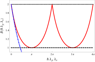
Figure 1: (Color online). The upper bound $\mathcal{B}(\hbar\lambda_{x}\lambda_{p})$ (solid, red line) with its upper (dotted, equal to $2$) and lower (dashed, equal to $1$) values emphasized. The blue dashed-dotted line represents the left hand side of (5) calculated for the Gaussian state discussed after Eq. (8).

Theorem 1.

The sum of squared moduli of the position and momentum characteristic functions is upper bounded:

$$|\Phi(\lambda_{x})|^{2}+|\tilde{\Phi}(\lambda_{p})|^{2}\leq\mathcal{B}(\hbar\lambda_{x}\lambda_{p}),$$ (5)

by

$$\mathcal{B}(\gamma)=2\sqrt{2}\frac{\sqrt{2}-\sqrt{1-\cos\left(\gamma\right)}}{1+\cos\left(\gamma\right)}.$$ (6)

The characteristic function is a linear functional of the probability distribution, so its modulus squared is convex. Since any quantum state can be written as a convex sum of pure states, the ChUR (5) is satisfied by all mixed states. Moreover, the above result can be immediately generalized to the multidimensional scenario in which (1) is defined as a $d^{N}\!x$ integral with $e^{i\boldsymbol{\lambda}\cdot\boldsymbol{x}}$. In that case, Eq. 5 remains valid with $\lambda_{x}$ ($\lambda_{p}$) relpaced by $\boldsymbol{\lambda}_{x}$ ($\boldsymbol{\lambda}_{p}$), and consequently $\lambda_{x}\lambda_{p}$ replaced by the scalar product $\boldsymbol{\lambda}_{x}\cdot\boldsymbol{\lambda}_{p}$.

We will provide an outline of the proof below. First, let us discuss the function $\mathcal{B}\left(\cdot\right)$ in inequality (5), which depends on the dimensionless parameter $\hbar\lambda_{x}\lambda_{p}$, and is plotted in Fig. 1. The upper bound is clearly periodic and varies between $1$ and $2$, the latter being the trivial value. When $\hbar\lambda_{x}\lambda_{p}=2k\pi$ for any integer $k$ we have $\mathcal{B}(2k\pi)=2$, and Eq. (5) gives no restriction on the sum of characteristic functions. This fact is a non-trivial emanation OurMasks of the full commutativity of spectral position and momentum projections Projections . In other words, the trivial bound equal to $2$ is saturated by a distribution $\rho\left(x\right)$ that is a (normalized) version of the Dirac comb (wave function being the proper limit of the sum of shifted Gaussians) with period $2\pi/\lambda_{x}$. The characteristic function $\Phi(\lambda_{x})$ is equal to $1$ in this case. At the same time, $\tilde{\Phi}(\lambda_{p})$ is the auto–correlation function of the comb with the related correlation parameter $\hbar\lambda_{p}$. In this case $\hbar\lambda_{p}=2k\pi/\lambda_{x}$, so this parameter fits the comb period, giving $\tilde{\Phi}(\lambda_{p})=1$. In the “opposite” situation, when $\hbar\lambda_{x}\lambda_{p}=\left(2k+1\right)\pi$ the upper bound reaches its minimal value $1$. This case captures the maximal non-compatibility of the position/momentum couple since both wave functions $\psi\left(x\right)$ and $\tilde{\psi}\left(p\right)$ cannot be simultaneously well auto–correlated.

Before we prove Theorem 1 we would also like to show that the UR (5) is stronger than the HUR. To this end we parametrize $\lambda_{x}=\sqrt{a}/b$ and $\lambda_{p}=\sqrt{a}b/\hbar$, where $a$ is a non-negative dimensionless parameter and $b$ denotes a parameter with unit of position. By taking the square of inequality (4) and neglecting the positive contributions of order $\sigma^{4}$, one immediately arrives at $|\Phi(\lambda_{x})|^{2}\geq 1-\lambda_{x}^{2}\sigma_{x}^{2}$, and the similarly for $|\tilde{\Phi}(\lambda_{p})|^{2}$. This lower bound together with the above parametrization weakens inequality (5) to the form

$$2-a\left(b^{-2}\sigma_{x}^{2}+\left(b/\hbar\right)^{2}\sigma_{p}^{2}\right)\leq\mathcal{B}(a).$$ (7)

Since for $a\geq 0$, $\mathcal{B}(a)=2-a+\mathcal{O}(a^{2})$, the above relation divided by $a$ implies in the limit $a\rightarrow 0$ that

$$1\leq b^{-2}\sigma_{x}^{2}+\left(b/\hbar\right)^{2}\sigma_{p}^{2}.$$ (8)

The minimum of the right hand side occurs for $b=\sqrt{\hbar\sigma_{x}/\sigma_{p}}$ and gives the HUR. Thus, the ChUR (5) is strictly stronger than the Heisenberg Uncertainty Relation. By a straightforward calculation one can check that the left hand side of (5) in the case of $\psi(x)$ being a Gaussian state and with all the above assignments (for $\lambda_{x}$, $\lambda_{p}$ and $b$) is equal to $2e^{-a/2}$. In the limit $a\rightarrow 0$, the Gaussians saturate the bound as can be seen in Fig. 1.

Proof.

Let us now outline the proof of Theorem 1. We start by taking three vectors $\left|\xi_{1}\right\rangle=\left|\Psi\right\rangle$, $\left|\xi_{2}\right\rangle=e^{i\lambda_{x}\hat{x}}\left|\Psi\right\rangle$ and $\left|\xi_{3}\right\rangle=e^{i\lambda_{p}\hat{p}}\left|\Psi\right\rangle$ with $\left|\Psi\right\rangle$ being normalized. The positive semi-definite, hermitian Gram matrix of this set of vectors is equal to

$$G=\left(\begin{array}[]{ccc}1&\Phi(\lambda_{x})&\tilde{\Phi}(\lambda_{p})\\ \Phi^{*}(\lambda_{x})&1&\Omega\\ \tilde{\Phi}^{*}(\lambda_{p})&\Omega^{*}&1\end{array}\right),$$ (9)

where $\Omega=\left\langle\Psi\right|e^{-i\lambda_{x}\hat{x}}e^{i\lambda_{p}\hat{p}}\left|\Psi\right\rangle$. The condition of positive-semi-definiteness of $G$ leads to a single nontrivial inequality $\det G\geq 0$ which explicitly reads

$$1-\Lambda-\left|\Omega\right|^{2}+\Theta+\Theta^{*}\geq 0,$$ (10)

where (we omit here the $\lambda$ arguments) $\Lambda=|\Phi|^{2}+|\tilde{\Phi}|^{2}$ and $\Theta=\Omega\Phi\tilde{\Phi}^{*}$. Consider now the parity transformation $\lambda_{x}\mapsto-\lambda_{x}$ and $\lambda_{p}\mapsto-\lambda_{p}$. A basic property of the characteristic function is that $\Phi(-\lambda)=\Phi^{*}(\lambda)$. Moreover, the well known Baker–Campbell–Hausdorff formula (equivalent to the Weyl commutation relations)

$$e^{i\lambda_{p}\hat{p}}e^{-i\lambda_{x}\hat{x}}=e^{-i\hbar\lambda_{x}\lambda_{p}}e^{-i\lambda_{x}\hat{x}}e^{i\lambda_{p}\hat{p}},$$ (11)

provides the transformation rule $\Omega\mapsto e^{-i\hbar\lambda_{x}\lambda_{p}}\Omega^{*}$. The terms $\Lambda$ and $\left|\Omega\right|^{2}$ present in (10) are thus invariant with respect to the above transformation, while $\Theta\mapsto e^{-i\hbar\lambda_{x}\lambda_{p}}\Theta^{*}$. Obviously, Eq. (10) must also hold for the transformed quantities.

If we now take the arithmetic mean of (10) together with its transformed counterpart, we will obtain an inequality of almost exactly the same form as (10), with the only difference that $\Theta$ is now multiplied by a complex constant $Z$ (i.e. $\Theta\mapsto Z\Theta$ ) of the form $Z=\frac{1}{2}(1+e^{i\hbar\lambda_{x}\lambda_{p}})$. In the final steps we resort to the fact that $Z\Theta\leq|Z|\left|\Theta\right|$ and the arithmetic-geometric mean inequality $\left|\Theta\right|\leq\frac{1}{2}\left|\Omega\right|\Lambda$. The same procedure is applied to the second, conjugated term $Z^{*}\Theta^{*}$. The above derivation leads to an inequality $1-\Lambda-\left|\Omega\right|^{2}+\left|Z\right|\left|\Omega\right|\Lambda\geq 0$ which after a single rearrangement is brought to the form

$$\Lambda\leq\frac{1-\left|\Omega\right|^{2}}{1-\left|Z\right|\left|\Omega\right|}.$$ (12)

Since the parameter $0\leq|\Omega|\leq 1$ can in principle assume any value, we maximize the right hand side of the above inequality with respect to it. The global maximum is found at $|\Omega|=(1-\sqrt{1-\left|Z\right|^{2}})/\left|Z\right|$, and leads to the final result presented in Theorem 1, where the identity $\left|Z\right|^{2}=\frac{1}{2}[1+\cos(\hbar\lambda_{x}\lambda_{p})]$ has been utilized. ∎

Let us mention that if one starts the proof with an alternative choice $\left|\xi_{2}^{\prime}\right\rangle=\hat{x}\left|\Psi\right\rangle$ and $\left|\xi_{3}^{\prime}\right\rangle=\hat{p}\left|\Psi\right\rangle$, the counterpart of inequality (10) is equivalent to the Robertson–Schrödinger uncertainty relation. Since in the current case we deal with non-hermitian displacement operators, such trivial correspondence does not occur.

ChUR and Quantum Optics—

Though the displacement operator does not correspond to an observable, its mean value can be measured directly in a quantum optical experiment if an ancillary qubit is used. Consider the quantum circuit shown in Fig. 2. The qubit is initialized in the $\left|{+}\right\rangle$ state, where $\left|{\pm}\right\rangle=(\left|{0}\right\rangle\pm{\left|{1}\right\rangle})/\sqrt{2}$ are the eigenstates of the Pauli operator $\hat{\sigma}_{x}$. The quantum system of interest is in the arbitrary state $\hat{\rho}$. The logic gate is a controlled displacement operator, defined by

$$\left|{0}\right\rangle\left\langle{0}\right|\hat{1}+\left|{1}\right\rangle\left\langle{1}\right|e^{i\lambda_{p}\hat{p}},$$ (13)

where the displacement is along the $x$ direction. Detecting the qubit in the $\pm$ basis gives the probabilities

$$P_{\pm}=\frac{1}{2}(1\pm\langle\cos(\lambda_{p}\hat{p})\rangle_{\hat{\rho}}).$$ (14)

Detecting the qubit in the $\hat{\sigma}_{y}$ basis, defined by eigenstates $\left|{\pm i}\right\rangle=(\left|{0}\right\rangle\pm i{\left|{1}\right\rangle})/\sqrt{2}$, gives

$$P_{\pm i}=\frac{1}{2}(1\mp\langle\sin(\lambda_{p}\hat{p})\rangle_{\hat{\rho}}).$$ (15)

Then the characteristic function can be obtained by combining the measurement results, since $\langle e^{i\lambda_{p}\hat{p}}\rangle_{\hat{\rho}}=P_{+}-P_{-}-iP_{-i}+iP_{+i}$. This type of qubit-assisted measurement scheme can be realized using existing technologies in several different platforms CavityQED ; hormeyll14 .

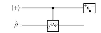
Figure 2: Quantum circuit to measure the characteristic function of $\rho(x)$ directly.

As an application of Theorem 1 in Quantum Optics we describe the mutual incompatibility of measurements made in position and momentum space using detectors with arbitrary apertures. In our analysis we discuss a very general model, in which the detection aperture is described by an arbitrary transmittance function $M\left(x\right)$. For single photons, for example, this detection scheme is implemented by the propagation through a general amplitude (and phase) spatial mask modelled by $\mathcal{A}(x)=A(x)e^{i\phi(x)}$, followed by its subsequent measurement with a full multi-mode detector Tasca13c . The aperture function $0\leqslant A(x)\leqslant 1$ provides $M(x)=|\mathcal{A}(x)|^{2}\equiv A^{2}(x)$ while the mask phase profile $\phi(x)$ does not affect the transmittance. The probability $\mathcal{Q}\left(y\right)$ that the quantum particle is detected with this mask function is then given by

$$\mathcal{Q}\left(y\right)=\int_{\mathbb{R}}\!dxM\left(x+y\right)\rho(x),$$ (16)

where $y$ can be thought of as the location parameter that defines the mask. For example, if the mask is an aperture of size $\delta$ (in some experimentally relevant units), then $M\left(x\right)$ might be chosen to be equal $1$ for $0\leq x\leq\delta$ and $0$ elsewhere. In that case (16) is simply the probability of finding a quantum particle on the interval $\left[-y,\delta-y\right]$.

A similar construction can be done in the momentum picture. One only needs a parameter $\kappa$ mapping the momentum variable into the position space, so that $\kappa p$ is a position-like variable. To have the readout function depending on the position-like variable we define the counterpart of (16) as follows

$$\mathcal{P}\left(y\right)=\int_{\mathbb{R}}\!dpM\left(\kappa p+y\right)\tilde{\rho}(p).$$ (17)

By calculating the ordinary Fourier transform [like in Eq. (2), but with $\hbar=1$ and the conjugate parameter $\lambda$ in units of inverted position] of both detection probability functions we obtain $\tilde{\mathcal{Q}}(\lambda)=\tilde{M}(\lambda)\Phi(\lambda)$ and $\tilde{\mathcal{P}}(\lambda)=\tilde{M}(\lambda)\tilde{\Phi}(\kappa\lambda)$. We are thus in position to propose a general uncertainty relation for detection masks:

$$\int_{\mathbb{R}}\!dy\left(|\mathcal{Q}(y)|^{2}+|\mathcal{P}(y)|^{2}\right)\leq\int_{\mathbb{R}}\!d\lambda|\tilde{M}(\lambda)|^{2}\mathcal{B}\left(\hbar\kappa\lambda^{2}\right).$$ (18)

The above result should prove useful in studies devoted to quantum aspects of EPR-based ghost imaging EPRghost and security protocols for compressive quantum imaging compresive2 ; compresive . A "periodic" variant of Eq. (18) (when $M(x)$ is a periodic function) is already applied in experimental entanglement detection with periodic amplitude masks OurMasks .

The derivation of (18) is very simple. Due to Parseval’s theorem from Fourier analysis, the left hand side translates directly to the $\lambda$-domain. To obtain the right hand side we apply the UR for characteristic functions from Theorem 1, with $\lambda_{x}=\lambda$ and $\lambda_{p}=\kappa\lambda$. It is worth mentioning that Eq. 18 remains valid for any complex–valued function $M(x)$.

ChUR and various theories in physics—

Besides its fundamental interest, the ChUR derived in this paper is related to several issues across various fields of physics. First of all, our approach remains valid with $\Phi(\lambda_{x})$ and $\tilde{\Phi}(\lambda_{p})$ substituted by $\left\langle\Psi\right|U\left|\Psi\right\rangle$ and $\left\langle\Psi\right|W\left|\Psi\right\rangle$, whenever the unitary matrices $U$ and $W$ satisfy the Weyl-type commutation relations $UW\!=\!e^{i\phi}WU$. A prominent example provided by Schwinger Schwinger and given by $\phi=2\pi/d$, where $d$ is the dimension of the Hilbert space, is a sort of prerequisite for the fruitful theory of Mutually Unbiased Bases.

Moreover, since Theorem 1 involves operators of the form $e^{i\lambda\hat{O}}$ it becomes valuable when the operator $\hat{O}$ does not exist itself (consequences of so called Stone–von Neumann theorem). A particularly interesting example of the number-phase uncertainty CN ; Luis2 ; Shepard (phase operators are not well defined) has just been described Luis along the lines of Theorem 1. Here we would like to briefly touch upon the broad theory of Loop Quantum Gravity , in which the so called Ashtekar connection AshtekarOld $A_{a}^{i}(x)$ plays the role of the canonical "position" variable in a field-theoretical sense . While moving to a quantum description, the problem appears as there is no local operator $\hat{A}_{a}^{i}(x)$, and one needs to resort to unitary holonomies. The standard approach to quantum uncertainty relations cannot thus be directly applied, however one can involve the Weyl algebra WeylLQG and use Theorem 1.

To explain better the idea behind the above prescription, we would like to discuss a very simple case from the field of Loop Quantum Cosmology. To this end we start with the well known FLRW metric

$$ds^{2}=-c^{2}dt^{2}+a^{2}(t)d\Sigma^{2},$$ (19)

where $a(t)$ denotes the dimensionless scale factor and $\Sigma$ refers to the 3-dimensional space. We further recall two time-dependent variables Ashtekar2 : $b=\dot{a}/a$ and $V=V_{0}a^{3}$, denoting the Hubble parameter and the physical volume of the expanding Universe respectively ($V_{0}$ is the coordinate volume). These variables satisfy the following Poisson bracket relation Ashtekar2

$$\left\{b,V\right\}=\pm 4\pi G/c^{2}\equiv Q,$$ (20)

where the $\pm$ sign depends on the orientation and is irrelevant in our considerations. If the operator $\hat{b}$ existed, then (20) would lead us to the UR: $\sigma_{b}\sigma_{V}\geq 4\pi\hbar G/c^{2}$ as stated in Eq. 11.21 of RovelliBook . Since the Ashtekar connection of this well-studied model is given by $A_{a}^{i}=\beta\dot{a}\delta_{a}^{i}$ , it becomes obvious that $b$ cannot be promoted to a quantum mechanical operator. As this limitation is not shared by the holonomy $U_{b}(\lambda_{b})=e^{i\lambda_{b}b}$, one can use $U_{b}$ together with $e^{i\lambda_{V}\hat{V}}$ and apply Theorem 1. In particular, if we set $\lambda_{V}=\pi/(\hbar Q\lambda_{b})$, so that the bound $\mathcal{B}$ is equal to $1$, and use (4) to extract the variance $\sigma_{V}^{2}$, the ChUR provides the uncertainty relation of the form:

$$\frac{4\hbar G}{c^{2}}\lambda_{b}\left|\left\langle U_{b}(\lambda_{b})\right\rangle\right|\leq\sigma_{V}.$$ (21)

The above UR is a formally right way of bounding the fluctuations of the volume of the Universe in terms of the volume shift operator $U_{b}$, relevant for understanding of the big-bang singularity Bojowald . Note also that this example actually represents Quantum Mechanics subject to the Bohr compactification. In other words, Theorem 1 is the only path towards URs in theories (such as Loop Quantum Cosmology Fewster ) with the Bohr compactification involved.

Looking into future, a further development of the discrete counterpart of the presented theory might bring useful results, for instance, in compressed sensing, as the Dirac comb state has no counterpart in various discrete systems. Generalizations of URs for the electromagnetic field (as discussed in Ashtekar1 ) might bring a better physical insight into the role played by Gauss linking numbers, or contribute to a better understanding of quantum effects for the gravitational field in a hot universe IBBPRD . We also believe that our approach will be influential to the theory of quantum optical characteristic functions. Questions about non-classicality of light are being asked and studied Agudelo1 in terms of the characteristic $P$-function reconstructed from the data accessible in experiments Agudelo2 , with a relevant filtering procedure based on auto-correlations Agudelo3 .

- (1) W. Heisenberg, Z. Phys. 43, 172 (1927).
- (2) E. Kennard, Z. Phys. 44, 326 (1927).
- (3) H. Robertson, Phys. Rev. 34, 163 (1929).
- (4) K. Korzekwa, M. Lostaglio, D. Jennings, and T. Rudolph, Phys. Rev. A 89, 042122 (2014).
- (5) S. Friedland, V. Gheorghiu, and G. Gour, Phys. Rev. Lett. 111, 230401 (2013).
- (6) Z. Puchała, Ł. Rudnicki, and K. Życzkowski, J. Phys. A 46, 272002 (2013).
- (7) P. Coles and M. Piani, Phys. Rev. A 89, 022112 (2014).
- (8) Ł. Rudnicki, Z. Puchała, and K. Życzkowski, Phys. Rev. A 89, 052115 (2014).
- (9) G. M. Bosyk, S. Zozor, M. Portesi, T. M. Osán, and P. W. Lamberti, Phys. Rev. A 90, 052114 (2014).
- (10) S Zozor, G. M. Bosyk, and M. Portesi, J. Phys. A: Math. Theor. 47, 495302 (2014)
- (11) J. Kaniewski, M. Tomamichel, and S. Wehner, Phys. Rev. A 90, 012332 (2014).
- (12) F. Buscemi, M. J. W. Hall, M. Ozawa, and M. M. Wilde, Phys. Rev. Lett. 112, 050401 (2014).
- (13) V. Narasimhachar, A. Poostindouz, and G. Gour, arXiv:1505.02223 (2015).
- (14) Ł. Rudnicki, S. P. Walborn, and F. Toscano, Europhys. Lett. 97, 38003 (2012)
- (15) Ł. Rudnicki, S. P. Walborn, and F. Toscano, Phys. Rev. A 85, 042115 (2012).
- (16) Ł. Rudnicki, Phys. Rev. A 91, 032123 (2015).
- (17) P. Busch, T. Heinonen, P. Lahti, Phys. Rep. 452, 155 (2007).
- (18) I. Białynicki-Birula and J. Mycielski, Commun. Math. Phys. 44, 129 (1975).
- (19) J. Solomon Ivan, N. Mukunda, and R. Simon, J. Phys. A: Math. Theor. 45, 195305 (2012).
- (20) P. Sánchez-Moreno, R. González-Férez, and J. S. Dehesa, New J. Phys. 8, 330 (2006).
- (21) Ł. Rudnicki, Phys. Rev. A 85, 022112 (2012).
- (22) I. Bialynicki-Birula and Z. Bialynicka-Birula, Phys. Rev. Lett. 108, 140401 (2012).
- (23) I. Bialynicki-Birula and Z. Bialynicka-Birula, Phys. Rev. A 86, 022118 (2012).
- (24) P. Busch, P. Lahti, and R. F. Werner, Phys. Rev. Lett. 111, 160405 (2013).
- (25) K. Fujikawa, Phys. Rev. A 85, 062117 (2012).
- (26) J. Erhart, S. Sponar, G. Sulyok, G. Badurek, M. Ozawa, and Y. Hasegawa, Nat. Phys. 8, 185 (2012).
- (27) S.-Y. Baek, F. Kaneda, M. Ozawa, and K. Edamatsu, Sci. Rep. 3, 2221 (2013).
- (28) A. S. Majumdar and T. Pramanik, Some applications of uncertainty relations in quantum information, arXiv:1410.5974 (2014).
- (29) F. Grosshans and N. J. Cerf, Phys. Rev. Lett. 92, 047905 (2004).
- (30) C. Branciard, E. G. Cavalcanti, S. P. Walborn, V. Scarani, and H. M. Wiseman, Phys. Rev. A 85, 010301 (2012).
- (31) R. Simon, Phys. Rev. Lett. 84, 2726 (2000).
- (32) S. P. Walborn, B. G. Taketani, A. Salles, F. Toscano, and R. L. de Matos Filho, Phys. Rev. Lett. 103, 160505 (2009).
- (33) A. Saboia, A. T. Avelar, S. P. Walborn, F. Toscano, arXiv:1407.7248 (2014).
- (34) M. D. Reid, Phys. Rev. A 40, 913 (1989).
- (35) H. M. Wiseman, S. J. Jones, and A. C. Doherty, Phys. Rev. Lett. 98, 140402 (2007).
- (36) E. G. Cavalcanti, S. J. Jones, H. M. Wiseman, and M. D. Reid, Phys. Rev. A 80, 032112 (2009).
- (37) S. P. Walborn, A. Salles, R. M. Gomes, F. Toscano, and P. H. Souto Ribeiro, Phys. Rev. Lett. 106, 130402 (2011).
- (38) J. Schneeloch, C. J. Broadbent, S. P. Walborn, E. G. Cavalcanti, and J. C. Howell, Phys. Rev. A 87, 062103 (2013).
- (39) Y. Aharonov, S. Massar, and S. Popescu, Phys. Rev. A 66, 052107 (2002).
- (40) M. Zych, F. Costa, I. Pikovski, and Č. Brukner, Nat. Commun. 2, 505 (2011).
- (41) N. G. Ushakov, J. Math. Sci. 84, 1179 (1997).
- (42) L. V. Rozovsky, Theory Probab. Appl. 44, 588 (2000).
- (43) W. Matysiak and P. J. Szablowski, J. Math. Sci. 105, 2594 (2001).
- (44) C.-Y. Hu and G. D. Lin, J. Math. Anal. Appl. 309, 336 (2005).
- (45) S. G. Bobkov, G. P. Chistyakov, and F. Götze, Electron. Commun. Probab. 17, 1 (2012).
- (46) Irina Shevtsova, J. Math. Anal. Appl. 418, 185 (2014).
- (47) N. G. Ushakov, Selected Topics in Characteristic Functions, VSP, Utrecht, 1999.
- (48) S. Luo, Z.Wang, and Q. Zhang, J. Phys. A: Math. Gen. 35, 5935 (2002).
- (49) D. S. Tasca, Ł. Rudnicki, R. S. Aspden, M. J. Padgett, P. H. Souto Ribeiro, and S. P. Walborn, “Testing for entanglement with periodic images, arXiv:1506.01095 (2015).
- (50) P. Busch and P. Lahti, Phys. Lett. A 115, 259 (1986).
- (51) J. Casanova, C. E. Lopez, J. J. Garcia-Ripoll, C. F. Roos, and E. Solano, Eur. Phys. J. D. 66, 222 (2012).
- (52) M. Hor-Meyll, J. O. de Almeida, G. B. Lemos, P. H. S. Ribeiro, and S. P.Walborn, Phys. Rev. Lett. 112, 053602 (2014).
- (53) D. S. Tasca, R. S. Aspden, P. A. Morris, G. Anderson, R. W. Boyd and M. J. Padgett, Opt. Express 21, 30460–30473 (2013).
- (54) R. S. Aspden, D. S. Tasca, R. W. Boyd, and M. J. Padgett, New J. Phys. 15, 073032 (2013).
- (55) G. A. Howland and J. C. Howell, Phys. Rev. X 3 011013 (2013).
- (56) D. J. Lum, S. H. Knarr, and J. C. Howell, Fast-Hadamard Transforms for Compressive Sensing of Joint-Systems: Measurement of a 16.8 Million-Dimensional Entangled Probability Distribution, arXiv:1505.05431 (2015).
- (57) J. Schwinger, Proc. Nat. Acad. Sci. U.S.A. 46, 570 (1960).
- (58) S. R. Shepard, Phys. Rev. A 90, 062117 (2014).
- (59) P. Carruthers and M. Martin Nieto, Rev. Mod. Phys. 40, 411 (1968).
- (60) P. Matía-Hernando and A. Luis, Phys. Rev. A 84, 063829 (2011).
- (61) A. Luis, Phase-number uncertainty from Weyl commutation relations, arXiv:1509.08085 (2015).
- (62) A. Ashtekar, Phys. Rev. Lett. 57, 2244 (1986).
- (63) C. Rovelli and F. Vidotto, Covariant Loop Quantum Gravity, Cambridge University Press, Cambridge, 2015
- (64) C. Fleischhack, Commun. Math. Phys. 285, 67 (2009).
- (65) A. Ashtekar and P. Singh, Class. Quantum Grav. 28, 213001 (2011).
- (66) M. Bojowald, Phys. Rev. Lett. 86, 5227 (2001).
- (67) C. J Fewster and H. Sahlmann, Class. Quant. Grav 25, 225015 (2008).
- (68) A. Ashtekar and A. Corichi, Phys. Rev. D 56, 2073 (1997).
- (69) I. Bialynicki-Birula, Quantum fluctuations of geometry in hot Universe, arXiv:1501.07405 (2015).
- (70) S. Ryl, J. Sperling, E. Agudelo, M. Mraz, S. Köhnke, B. Hage, and W. Vogel, Uniified Nonclassicality Criteria, arXiv:1505.06089 (2015).
- (71) E. Agudelo, J. Sperling, W. Vogel, S. Köhnke, M. Mraz, B. Hage, Continuous sampling of the squeezed state nonclassicality, arXiv:1411.6869 (2015).
- (72) E. Agudelo, J. Sperling, and W. Vogel, Phys. Rev. A 87, 033811 (2013).