Nonlinear dynamics of the mammalian inner ear

Abstract

A simple nonlinear transmission-line model of the cochlea with longitudinal coupling is introduced that can reproduce Basilar membrane response and neural tuning in the chinchilla. It is found that the middle ear has little effect on cochlear resonances, and hence conclude that the theory of coherent reflections is not applicable to the model. The model also provides an explanation of the emergence of spontaneous otoacoustic emissions (SOAEs). It is argued that SOAEs arise from Hopf bifurcations of the transmission-line model and not from localized instabilities. The paper shows that emissions can become chaotic, intermittent and fragile to perturbations.

Significance: The cochlea is a remarkable device that out-performs any human-made system; it is sensitive to sounds over a million-fold intensity and a ten-octave frequency range, and can distinguish signals separated by microseconds at frequencies only 0.2% apart. Here we study the mechanisms that make this work. We present a nonlinear mathematical model that combines the key physiological processes, including both longitudinal coupling and hair cell motility, which produces response patterns that agree with experiments in different animals. A dynamical systems analysis of the model allows us challenge existing theories on the source of spontaneous otoacoustic emissions, suggesting that the entire organ, rather than localized instabilities, are key.

The mammalian hearing organ is a sensitive sensory device that operates at the extremes of physical limits. It is capable of resolving sound pressure levels just above atmospheric thermal noise and of discriminating frequencies 0.2% apart Hudspeth2000 . In order to achieve these features the inner ear employs an active feedback mechanism Gold1948 . Like any feedback loop, it is possible for the one in the inner ear to become unstable. In this paper we show how such an instability can lead to self-excited oscillations that are emitted from the ear as sound, which we propose as a mechanism for the generation of spontaneous otoacoustic emissions (SOAEs) Kemp1979 . We derive this from a new mathematical model of the mammalian ear, which includes both active somatic motility and longitudinal coupling in the cochlea, linked to the atmosphere via the middle ear.

One widespread explanation of emission generation is due to Shera Shera2003 , Shera and Zweig ZweigShera1995 and Talmadge et al. Talmadge1998 . They argue that spontaneous emissions are wave instabilities that arise because of coherent reflection at the stapes and at the characteristic frequency (CF) position of the cochlea; a mechanism that gives rise to standing waves that are stabilized by the cochlear nonlinearities. However, this theory is based on linear properties of the cochlea and does not explain how standing waves are stabilized.

Here, we apply the theory of dynamical systems to revisit the question of SOAEs, which leads to an alternative explanation for emission generation. We show that stability loss in the model generically corresponds to a Hopf bifurcation Kuznetsov2004 , which can lead to a sustained periodic emission. This is different from the so-called ‘Hopf ear’ Eguiluz2003 , in that it is an emergent macro-level property of the cochlear model, with all its many interconnected elements, rather than being localized in any individual micro-scale component. Indeed, one advantage of our approach is that there is no need to assume, a priori, the mechanism of the stability loss; bifurcation theory determines the onset of instability irrespective of its source. We further predict that these bifurcations are ubiquitous, provided there is fine-scale spatial variation of the cochlear parameters. This finding provides a consistent explanation for widespread observation of SOAEs; in realistic operating conditions a bifurcation point is never far away. As one goes beyond a Hopf bifurcation, the resulting small amplitude limit-cycle vibrations can grow in amplitude, deform, and undergo further instabilities and bifurcations. One possible physical manifestation of such complex motions is in the way emissions can appear, disappear or change their character as the cochlea undergoes changes due to damage Veuillet2001 or aging Kohler1992 , for example.

While linear cochlear models can also predict instability, they cannot adequately explain what happens when multiple instabilities produce a multiple independent periodic motions. In a linear system, multiple oscillations can coexist without any effect on each other. In nonlinear systems, such as the model we present here, we expect more complex phenomena to arise, such as intermittent or chaotic oscillations to arise, for which there is some experimental evidence. For example, Burns Burns2009 describes experimentally observed short-term property changes to SOAEs, including their seemingly random sudden appearance and disappearance. Keefe et al. Keefe1990 used time series analysis methods that could distinguish chaotic spontaneous as well as stimulated emissions. It is though perhaps not surprising that there are not more reports of intermittent or chaotic SOAEs. To eliminate environmental noise one must use temporal averaging. However, averaging can also mask short term spectral variations and chaos.

The rest of this paper is organized as follows. First, we introduce our mathematical model. Then we show how the model reproduces chinchilla BM mechanical data and neural tuning. Applying spatial roughness to the feedback coefficients of the model, we show that the cochlea develops resonances. As we increase the size of the roughness the resonances turn into instabilities and we observe spontaneous oscillations. We investigate these vibrations in detail and conclude that our model can produce complicated dynamics in line with experimental observations.

I Nonlinear transmission-line model of the inner ear

We start from a simple transmission-line model of the cochlea inspired by the work of Zweig Zweig1991 . Our model, instead of a delayed feedback, contains a distributed feed-forward mechanism to account for the organ of Corti (OOC) structure. This type of active mechanism was introduced by Geisler Geisler1993 and Steele and Lim SteeleLim1999 and successfully applied in many models. Moreover, parameters of such a model are easily interpreted in terms of the longitudinal coupling within the OOC Yoon2011 . In SzalaiJoMMS together with Epp, we showed how such spatial coupling can be directly compared with time-delayed feedback, but with better stability properties.

As is common in modeling the mechanics of the cochlea, we assume that the fluid in the perilymph is incompressible and inviscid, which yields a wave equation for the pressure difference $p$ between the scala tympani and vestibuli, and the Basilar membrane (BM) displacement $x_{\mathrm{bm}}$,

$$\ddot{x}_{\mathrm{bm}}(\xi,t)=\frac{\varepsilon^{2}}{m}\frac{\partial^{2}}{\partial\xi^{2}}p(\xi,t)$$ (1)

where dot denotes (partial) differentiation with respect to time $t$. We nondimensionalise the longitudinal distance $\xi$, so that the length of the cochlea becomes unity, $0\leqslant\xi\leqslant 1$. The lumped parameter $\varepsilon$ is a function of the geometry of the cochlear chambers and the density of the perilymph fluid, and $m$ is the mass surface density of the BM.

Our model of the BM motion, and its amplification by outer hair cells (OHCs), is a simplified version of that developed by Ó Maoléidigh and Jülicher Daibhid2010 . This model accounts for the active nonlinearity of hair bundles, coupled to hair cell elongation, for a detailed derivation see SzalaiNonlin . To that model we add longitudinal coupling, as described in SzalaiJoMMS . Specifically, the BM displacement $x_{\mathrm{bm}}$ and OHC charge $q$, at longitudinal distance $\xi$ from the stapes, are defined by the equations

$$\ddot{x}_{\mathrm{bm}}(\xi,t) =\frac{1}{m}p(\xi,t)-2\zeta(\xi)\omega_{0}(\xi)\dot{x}_{\mathrm{bm}}(\xi,t)-\omega_{0}^{2}(\xi)x_{\mathrm{bm}}(\xi,t)$$

$$\quad-\frac{f_{q}\omega_{0}^{2}(\xi)}{L(\xi)}\int_{-L(\xi)}^{L(\xi)}w\left(\frac{h}{L(\xi)}\right)q\left(\xi-h,t\right)\mathrm{d}h,$$ (2)

$$\dot{q}(\xi,t) =-\gamma q(\xi,t)+\nu\dot{x}_{bm}(\xi,t)$$

$$\quad+I_{\mathrm{hb}}\left(P_{\mathrm{O}}\left(\Delta\dot{x}_{\mathrm{bm}}(\xi,t)\right)-P_{\mathrm{O}}(0)\right).$$ (3)

The BM motion has natural frequency $\omega_{0}$ and relative damping $\zeta$, both of which we assume to depend on position $\xi$. The BM is forced both by the cochlear pressure difference $p$ at position $\xi$, and also by the OHCs which exert a force due to the unique protein called prestin Ashmore2008 embedded in its lateral wall. We assume that the effect of the OHCs is longitudinally distributed, due to the push-pull mechanism of the OOC Yoon2009 ; Yoon2011 , giving rise to the integral term on the right-hand side of (2). The longitudinal convolution kernel $w(x)$ is assumed to have a strong positive feed-forward and a weak negative feed-backward component,

$$w(x)=\operatorname{e}^{-\beta(x-\delta_{g})^{2}}\sin(x-\delta_{o}),$$

and a characteristic feed-forward distance is given by $L(\xi)=L_{0}\mathrm{e}^{\mu_{L}\xi}$, that is about twice as long at the apex than at the base. Note that the kernal $w$ resembles a strongly damped wave and therefore might alternatively represent a secondary transmission line generated in the tunnel of Corti Karavitaki2007 or on the tectoral membrane Ghaffari2007 .

The charge $q$ inside the OHC is controlled by the mechanically sensitive ion channels of the hair bundle Hudspeth2008 . Equation (3) models the capacitor of the OHC that integrates ion currents flowing through the ion channels. The OHC has an active mechanism to regain its resting potential, which is modeled by the rate constant $\gamma$. We assume that the open probability of the ion channels is described by a second-order Boltzmann function Lukashkin1998

$$P_{\mathrm{O}}=\left[1+\operatorname{e}^{-a_{1}(x-b_{1})}\left(1+\operatorname{e}^{-a_{2}(x-b_{2})}\right)\right]^{-1}.$$

The piezoelectric property of the OHC is represented by the constant $\nu$.

The boundary condition of the model at the apex is determined by the helicotrema, which we assume has no resistance to fluid motion, hence $p(1,t)=0$. The boundary condition at the base is determined by the action of the stapes on the oval window. The stapes is in turn controlled by the dynamics of the middle ear which we model as a single-degree-of-freedom oscillator

$$\ddot{x}_{\mathrm{ow}}+2\zeta_{\mathrm{ow}}\dot{x}_{\mathrm{ow}}+\omega_{\mathrm{ow}}^{2}x_{\mathrm{ow}}=m_{\mathrm{ow}}^{-1}\left(p(0,t)+Gp_{e}\right),$$ (4)

where $p_{e}$ is the sound pressure acting on the eardrum and the subscript ‘$ow$’ refers to the oval window. Hence the basal boundary condition can be determined from force balance to be

$$\frac{\partial p}{\partial\xi}(0,t)=mk_{\mathrm{ow}}\ddot{x}_{\mathrm{ow}}(t).$$

I.1 Parameter fitting

Table 1: Parameter values of the mathematical model

Parameter	Value	Description
$\varepsilon$	0.0594	cochlear geometry constant
$m$	$0.0055\text{\,}\mathrm{g}\usk\mathrm{c}\mathrm{m}\rpsquared$	mass density of the Basilar membrane
$\omega_{0}$	$20.832\mathrm{e}^{-4.8354\xi}-0.1455$	undamped natural frequency of the Basilar membrane
$\zeta$	$0.11\mathrm{e}^{1.4\xi}$	relative damping of the Basilar membrane
$f_{q}$	0.2221	gain of the outer hair cell
$L$	$0.005\mathrm{e}^{0.7\xi}$	characteristic feed-forward distance
$\gamma$	$12.5\times 5^{-\xi}$ m s	RC time constant of the outer hair cell
$\nu$	$0.72\text{\,}\mathrm{nC}$	piezoelectric constant of the outer hair cell
$I_{\mathrm{hb}}$	$0.390323\text{\,}\mathrm{nA}$	maximum transduction current through the hair bundles
$a_{1}$	19.9873	parameter of $P_{\mathrm{O}}$
$a_{2}$	16.3928	parameter of $P_{\mathrm{O}}$
$b_{1}$	0.0692021	parameter of $P_{\mathrm{O}}$
$b_{2}$	0.0369987	parameter of $P_{\mathrm{O}}$
$m_{\mathrm{ow}}$	$1.85\text{\,}\mathrm{g}\usk\mathrm{c}\mathrm{m}\rpsquared$	surface density of the stapes
$k_{\mathrm{ow}}$	$1100\text{\,}\reciprocal{\mathrm{c}\mathrm{m}}$	coupling of oval window to perilymph
$\zeta_{\mathrm{ow}}$	0.265	relative damping of the middle ear
$\beta$	0.78	convolution kernel Gaussian characteristic width
$\delta_{g}$	0.74	convolution kernel Gaussian shift
$\delta_{o}$	$-$0.04	convolution kernel wave shift
$L_{0}$	0.005	feed-forward distance at base
$\mu_{L}$	0.7	rate of growth of the feed-forward distance

The model (1)-(4) is only complete once parameters have been specified; a full list is given in Table 1. We fitted the model to the frequency response function (FRF) of the BM at $0\text{\,}\mathrm{dB}$ sound pressure level (SPL) of animal N92 in the data of Rhode Rhode2007 . The sharpness of tuning was fitting simple exponential functions to $\zeta(\xi)$, $L(\xi)$ and $\gamma(\xi)$ and by finding a suitable value for $f_{q}$. The shape of the FRF was tuned by varying the parameters of $w(h)$, that is $\beta$, $\delta_{g}$ and $\delta_{o}$. However, tuning the model at a single position is not sufficient, because we want the sharpness of tuning to be accurate at every BM position. Unfortunately this type of data from a single cochlea does not currently exist. Reasoning that BM tuning and neural tuning are close, we instead use the neural tuning data of Recio-Spinoso et al. RecioSpinoso2005 to further fit the parameters $\zeta(\xi)$, $L(\xi)$ and $\gamma(\xi)$ of our model.

The nonlinear response of the model was tuned at the CF position of $6.6\text{\,}\mathrm{kHz}$ for the $6.6\text{\,}\mathrm{kHz}$ stimulus. Only the parameters $a_{1}$, $b_{1}$, $a_{2}$ and $b_{2}$ of the open probability function $P_{\mathrm{O}}$ were altered, while keeping the derivative at the equilibrium ${P}^{\prime}_{\mathrm{O}}(0)$ constant, so that the $0\text{\,}\mathrm{dB}$ FRF persisted. The sensitivity of the model is then tuned by adjusting only two parameters: $G$, which scales the input signal, and $\Delta$, which tunes the sensitivity of the hair bundles, and effectively determines the BM amplitude range.

II Results & Discussion

II.1 BM response

In order to find the BM response, we solve our model (1)-(4) numerically; see the Materials and Methods section for details. The results are presented in Fig. 1 in the form of thick colored lines. The superimposed thin black curves show the corresponding experimental data.

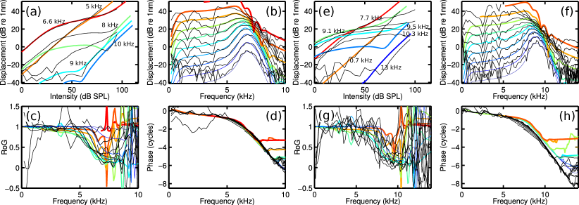
Figure 1: BM response of the model compared to data sets in Rhode2007 taken at the (a-d) CF $6.6\text{\,}\mathrm{kHz}$ position and (e-h) at the position with CF $9.1\text{\,}\mathrm{kHz}$. (a,e) BM displacement as a function of sound pressure level at different stimulus frequencies. (b,f) Frequency response functions at different SPLs, the lowest curve corresponds to 0 dB SPL. (c,g) Rate of growth indicating compression at different amplitudes as a function of frequency. (d,h) phase of the BM displacement. Thin black lines represent experimental data published in Rhode Rhode2007 and thick color lines represent numerical results. The bottom curve in (b-d) and (f-h) corresponds to 0 dB SPL, while consecutive curves (reading up) increase by 10 dB in SPL.

Results at the CF place of $6.6\text{\,}\mathrm{kHz}$, for which our model is tuned, are shown in Figure 1(a-d). Figures 1(a) and (b) show input–output functions; BM displacement as a function of sound pressure level (SPL) at various frequencies, and as a function of SPL at various frequencies, respectively. The data at lower than CF frequencies are accurately matched by the results, at higher than CF frequencies the calculated response is more compressed at lower SPLs than the data. The maximal compression rate, however, matches the data well. Figure 1(b) shows the frequency response functions at different SPLs. Again, the agreement with data is good. However, for higher amplitude stimuli the peak in the data widens almost symmetrically, while our calculations show almost the same width; this is the same disagreement as in Figure 1(a). One of the reasons why the peak of the tuning curve in our calculations does not broaden is because our convolution kernal $w$ does not depend on SPL. One way to improve the model would be to allow the parameters of $w$ to vary with $p_{e}$. Possible physical causes of such variation include tectoral membrane waves Ghaffari2007 and tunnel of Corti flow Karavitaki2007 .

Sound compression can be measured by the rate of growth (RoG), defined as the slope of the log-log graph of BM displacement versus SPL. Figure 1(c) shows the RoG, as a function of frequency, for a range of different stimulus intensities. Our model shows good agreement with the data. As expected, compression is minimal for frequencies significantly lower than CF, then increases (so that the RoG can be as low as $0.1$). Note that, due to interference, the RoG fluctuates significantly at certain frequencies especially above CF, which the model also reproduces. The phase variation of the BM response is illustrated in Figs. 1(d). Again we see good agreement between model predictions and experimental data.

Even though our model has been fitted to data from a specific animal whose BM vibration was measured at the $6.6\text{\,}\mathrm{kHz}$ CF position, we can compare its predictions to another dataset at a different frequency, measured in a different animal of the same species. Such data are shown in Figure 1(e-h). The model is adjusted by changing only two parameters: the input sensitivity $G$ and hair bundle sensitivity $\Delta$. The numerical results are still reasonably close to the data and all the qualitative features are preserved. The most obvious differences are that our model shows slightly sharper tuning than the animal, and that the phase variation along the frequency axis is somewhat greater in the experimental data (again possibly a result of the assumption that $w$ is independent of stimulus).

II.2 Stability of ideal and rough cochlea models

Having shown the validity of our model, we now use it to investigate the stability of the cochlea. Dynamical systems theory states that if the spectrum of the system at an equilibrium state has only negative real parts, the system is stable and small perturbations to that equilibrium will decay. Since our cochlea model (1)-(4) is a partial differential equation with spatial feedback and feed-forward, its spectrum will typically contain a continuous curve in the complex plane, spanning frequencies from the lowest to the highest audible frequencies. However, our use of a numerical discretization scheme (which approximates the system by a large set of ordinary differential equations) means that we can in practice compute the spectrum using a standard eigenvalue solver, resulting in a discrete approximation to the spectrum, with a large number of discrete eigenvalues.

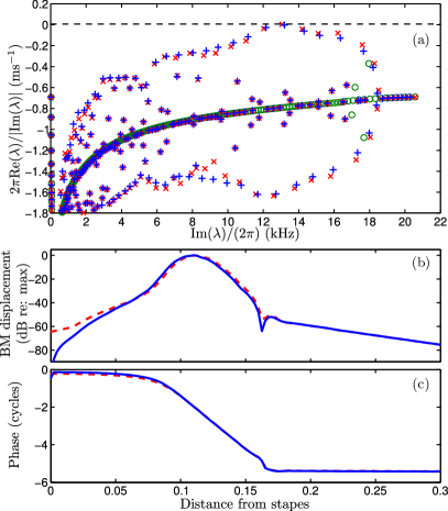
Figure 2: (a) Characteristic roots of the cochlear model. Green circles correspond to the smooth cochlea, red crosses to the rough cochlea with $\sigma=0.06$, and blue pluses represent a cochlea of the same roughness without the middle ear. The horizontal axis is the frequency of the characteristic root and the vertical axis is the relative damping, which is the log of the amplitude ratio of two consecutive periods of free vibration with the given frequency. (b,c) Magnitude and phase of the eigenvector corresponding to the most unstable eigenvalue, for the rough cochlea model; red dashed and solid blue lines correspond to models with and without the middle ear respectively.

Figure 2(a) shows computed spectra of the cochlea model, in the absence of stimulus. The imaginary axis is shown as a dashed line; any eigenvalue $\lambda$ above this line indicates instability of the cochlea. The green circles in Figure 2(a) (mostly organized in the thick line in the middle of the graph) represent the spectrum of the cochlea described above; they show that $\operatorname{Im}(\lambda)<0$ for all $\lambda$, so the cochlea is stable to small disturbances.

This calculation is for an ideal cochlea; a real organ will in general have small geometric variations of its properties along its length. In order to model such inhomogeneities, we allow the feed-forward parameter $f_{q}$ to vary randomly about its notional value at each position of the cochlea. We assume this variation to be normally distributed with zero mean and constant variance $\sigma^{2}$. Such randomness has been shown by Ku et al. Elliott2009 to induce reflections from the Basilar membrane back towards the stapes. In what follows we shall consider only one realization of the distribution, but we shall allow the variation to be scaled, in effect varying the standard deviation $\sigma$. We shall refer to such a model the rough cochlea, with $\sigma$ a measure of the degree of roughness.

The spectrum of one particular rough cochlea (with $\sigma=0.06$) is represented in Figure 2(a) by red $\times$ signs. We see that the continuous spectrum breaks up; the eigenvalues are scattered, and discrete eigenvalues jump out of the curve found for the smooth cochlea, sometimes by a significant distance. The closer an eigenvalue gets to the imaginary axis, the more the cochlea becomes sensitive to a disturbance at the corresponding frequency, which lowers the hearing threshold at that frequency. If an eigenvalue crosses the imaginary axis, a Hopf bifurcation occurs; as a result the cochlea becomes unstable and we would expect a spontaneous oscillation in the absence of any stimulus. This explains why SOAEs occur at the frequencies where the hearing threshold has notches. We also see in Figure 2(a) that spectral points close to the imaginary axis are roughly periodically spaced in frequency. This agrees with data that spontaneous and stimulus frequency OAEs and the hearing threshold microstructures are roughly periodic in frequency Kemp1981 .

II.3 Coherent reflections

The observation from Figure 2(a) that spectral points close to the imaginary axis are regularly spaced in frequency might be explained by the theory of Zweig and Shera ZweigShera1995 , whose assumption is that resonances build up in the cochlea between the oval window and the CF position of the resonance. To test such a hypothesis we removed the middle ear from our model altogether, and made sure that there is no reflection from the oval window by setting $p(0,t)=0$. Calculating the stability of this model, with the same roughness as before, yields a remarkably similar spectrum (illustrated by the blue $+$ signs in Figure 2(a)). This means that, while reflections from the oval window play a part in shaping resonances, they are not essential.

To further clarify how reflections occur we also calculated the eigenvector that corresponds to the largest $\mathrm{Re}(\lambda)/|\mathrm{Im}(\lambda)|$ value; shown in Figure 2(b,c), with and without the middle ear (red dashed and blue solid curves respectively). These correspond to the vibration pattern of the most unstable mode of the cochlea. It can be seen that the magnitude of the vibration rapidly decreases towards the base of the cochlea when the middle ear is removed. However, the BM pattern is remarkably similar to that with the intact middle ear for the rest of the cochlea.

To explore the implications of local reflections, we also considered the case when the longitudinal coupling parameter $f_{q}$ is increased by 20% at a single position, so that it forms a step function from base to apex, rather than varying randomly with length (data not shown). We might imagine that such an inhomogeneity will act as a single point of reflection. We found instead that distinct resonances were found (confirming the result in Ku et al. Elliott2009 ), and the cochlea patterns at the strongest resonance were indistinguishable from the result in Figure 2(b,c). We therefore conclude that the theory of coherent reflections is not adequate to explain our results.

II.4 Spontaneous emissions

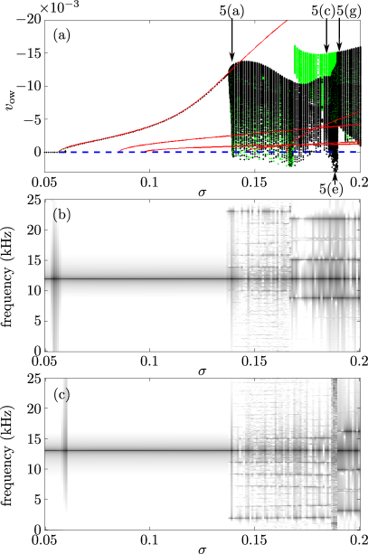
Figure 3: (a) Amplitude of spontaneous emissions calculated from the model, represented by oval window fluid velocity as a function of surface roughness. Red (periodic orbits) and blue (fixed point) curves denote the results of numerical continuation of the model. Black and green dots represent simulation results when increasing and decreasing $\sigma$, respectively. Points indicated by arrows represent responses plotted in detail in Figure 4. (b,c) Spectrograms of the cochlea emission with decreasing $\sigma$ and increasing $\sigma$ respectively.

We can also use our unforced cochlear model to quantify the nature of the spontaneous oscillations that exist beyond any point of instability. When an eigenvalue crosses the imaginary axis, as in the case of the rough unforced cochlea model described above, a Hopf bifurcation (of the entire cochlea) occurs; as a result, we expect a spontaneous oscillation to develop at approximately the frequency of the eigenvalue. Figure 3(a) shows the results of a combination of numerical continuation and simulation techniques to track both stable and unstable periodic orbits, and also to reveal more complicated dynamical behavior. The resting position of the cochlea is represented by a blue line, the solid portion representing where this is stable and the dashed portion where it is unstable. The red curves show the results of tracking the limit cycle motions born at a sequence of Hopf bifurcations that occur as the surface roughness $\sigma$ increases. shows a graph of the cochlear response as $\sigma$ varies. The vertical axis shows the stapes velocity $v_{ow}=\dot{x}_{ow}$ at the time instance when the stapes displacement is zero. This creates a sequence of values $v_{ow}$ which can be represented as a so-called Poincaré map $v_{ow}\mapsto P(v_{ow})$. Superimposed on the plot are the results of direct simulations, after any transient motion has decayed. These are represented by black and green dots. The black dots were obtained by making a slow forward sweep in $\sigma$ and the green dots by making a backward sweep. Corresponding spectrograms are shown in Figure 3(b,c).

Note from Figure 3(a) that as $\sigma$ increases from zero, the unforced cochlea goes unstable at around $\sigma=0.05$, via a supercritical Hopf bifurcation. Thus, a stable periodic orbit is born as $\sigma$ increases through this value. This represents a single frequency SOAE at $\approx$$13.072\text{\,}\mathrm{kHz}$, seen clearly in the spectrograms. Further supercritical Hopf bifurcations occur from the (now unstable) steady state as $\sigma$ increases further, although these branches of limit cycles all appear to be unstable. The single stable periodic solution can be inferred from where the where black dots of the simulation data overlie the red line from numerical continuation. The amplitude of this limit cycle grows steadily with $\sigma$.

Suddenly, for $\sigma\approx 0.13738$, the (single frequency) periodic orbit loses stability at $\sigma=0.13738$, through a supercritical secondary Hopf (or Neimark-Sacker) bifurcation. This creates quasi-periodic motion represented by the wide region of black dots in Figure 3(a). A second frequency $1.93\text{\,}\mathrm{kHz}$ is clearly visible in the spectrograms. At $\sigma\approx 0.168$ a second quasi-periodic orbit appears, with frequencies 3.16 and $13.06\text{\,}\mathrm{kHz}$, which coexists with the first for larger values of $\sigma$. The two different attractors are identified by different patterns of black and green dots in Figure 3(a) for $0.168<\sigma<0.186$, and different patterns in the spectrograms in Figure 3(b,c). At $\sigma\approx 0.186$ the first quasi-periodic orbit (black dots) breaks up to form a chaotic attractor; this is indicated by a sudden broadening of the spectrogram in Figure 3(c).

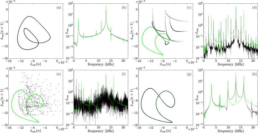
Figure 4: Poincare maps (a,c,e,g) and corresponding frequency spectra (b,d,f,h) of solutions of the cochlear model, for values of cochlear roughness $\sigma$ indicated in Figure 3(a). See text for details.

Figure 4 illustrates the qualitatively different classes of emissions predicted by the model in more detail, showing both the orbits (as Poincaré maps) and their spectra. The first quasi-periodic orbit, just after onset, is shown in Figure 4(a-b) and the two coexisting quasi-periodic orbits by green and black dots in Figure 4(c-d); note how the differing second frequencies result in different spacings between the peaks in the spectra. The chaotic attractor, shown with black dots in Figure 4(e-f) is of broadband character. Finally, the chaotic attractor disappears at $\sigma=0.1892$, where only a single quasi-periodic orbit remains, shown in Figure 4(g-h).

The scenario described above can change significantly when applying different roughness patterns to the feedback coefficient $f_{q}$. However, simulations with different realizations (not shown) suggest that the supercritical nature of the bifurcation remains, and that supercriticality is the property of the chosen open probability function $P_{\mathrm{O}}$. Changing $P_{\mathrm{O}}$ can result in a subcritical Hopf bifurcation, as reported in SzalaiMoH2011 .

The result that at a single parameter value multiple stable vibration patterns can coexist has implications for explaining other features observed experimentally. A large enough perturbation (e.g., a click) can push the ear into exhibiting different SOAE spectra, making one SOAE frequency appear and another disappear. Such changes are found experimentally Burns2009 , as are hallmarks of chaotic oscillations Keefe1990 , in qualitative agreement with the dynamics we predict.

III Conclusions

In this paper we have introduced a nonlinear transmission-line model of the mammalian hearing organ. We believe this to be the first mathematical model that is both able to capture the turning curves of the Basilar membrane across a range of different frequencies and come up with credible, testable explanations for observed finite-amplitude otoacoustic emissions. Specifically, the model provides a parsimonious synthesis of many of the features that have been proved important in previous modeling and experimental studies over several decades: fluid-structure interaction leading to waves that travel a frequency dependent distance to the characteristic frequency position along the Basilar membrane; longitudinal variation in organ of Corti properties; local nonlinearity due to the combined effects of outer hair cell somatic motility and hair bundle adaptation; and spatial feed-forward effects due to longitudinal coupling within the OOC.

The results in Figure 1 show how the combination of longitudinal coupling together with local nonlinearity is able to reproduce both qualitatively and quantitatively BM vibration data and neural tuning in different animals. We are not aware that models with either pure longitudinal coupling or pure local nonlinearity are able to reproduce such features.

Moreover, by applying a range of techniques from dynamical systems theory, we have been able to calculate both instability thresholds and the waveforms of post-instability spontaneous otoacoustic emissions. We have shown how the roughness of the cochlea can be responsible for producing these resonant instabilities. Moreover, by removing the middle ear and allowing no reflections at the oval window, we found that the resonance to only slightly diminish, but for the overall pattern of BM motion to be maintained. This shows that SOAEs can be produced by instabilities that do not require reflections from the middle ear. Reflections, however, might occur elsewhere.

Our model also how spontaneous OAEs arise robustly from supercritical Hopf bifurcations of the entire cochlea. Thus we do not need to make artificial “Hopf ear” hypotheses about local nonlinearities at a particular CF being responsible. Furthermore, with significant roughness, the model exhibits a range of complex emissions beyond pure tones including chaotic signals and bi-stability between different kinds of SOAE. These properties can explain reported recordings of emissions that appear to spontaneously switch between different signal patterns.

IV materials

IV.1 Equivalent formulation of the model

In order to be able to discretize our model into a set of ordinary differential equations, we first combine (1) and (2) to eliminate the pressure $p$

$$\ddot{x}_{\mathrm{bm}}-\varepsilon^{2}\frac{\partial^{2}}{\partial\xi^{2}}\ddot{x}_{\mathrm{bm}}=\left.\varepsilon^{2}\frac{\partial^{2}}{\partial\xi^{2}}\right(2\zeta\omega_{0}\dot{x}_{\mathrm{bm}}(\xi,t)+\omega_{0}^{2}x_{\mathrm{bm}}(\xi,t)\\ \left.+\frac{f_{q}\omega_{0}^{2}}{L}\int w(h/L)q\left(\xi-h,t\right)\,\mathrm{d}h\right).$$ (5)

Equation (3) stays unmodified. The governing equations of the middle ear are rewritten in state-space form using $x_{1}=x_{\mathrm{bm}}(0,t)$, $x_{2}=\dot{x}_{\mathrm{bm}}(0,t)$, $y_{1}=x_{\mathrm{ow}}$ and $y_{3}=\dot{x}_{\mathrm{ow}}-(m/m_{\mathrm{ow}})\dot{x}_{\mathrm{bm}}(0,t)$ as follows

$$\dot{y}_{1} =y_{3}+\kappa^{-1}x_{2},$$

$$\dot{y}_{3} =-\omega_{\mathrm{ow}}^{2}y_{1}-2\zeta_{\mathrm{ow}}\omega_{\mathrm{ow}}y_{3}+\kappa^{-1}\omega_{\mathrm{bm}}^{2}x_{1}+G_{e}p_{e},$$

$$\dot{x}_{1} =x_{2},$$

$$\dot{x}_{2}-\delta\frac{\partial}{\partial x}\dot{x}_{2} =\delta\frac{\partial}{\partial x}\left(2\zeta_{\mathrm{bm}}\omega_{\mathrm{bm}}x_{2}+\omega_{\mathrm{bm}}^{2}x_{1}\right)$$

$$\quad-\left(2\zeta_{\mathrm{bm}}\omega_{\mathrm{bm}}-2\zeta_{\mathrm{ow}}\omega_{\mathrm{ow}}\right)x_{2}-\omega_{\mathrm{bm}}^{2}x_{1}$$

$$\quad-\kappa\left(G_{e}p_{e}-2\zeta_{\mathrm{ow}}\omega_{\mathrm{ow}}y_{3}-\omega_{\mathrm{ow}}^{2}y_{1}\right),$$

where $\kappa=m_{\mathrm{ow}}/m$, $\delta=\kappa/k_{\mathrm{ow}}$ and $G_{e}=G/m_{\mathrm{ow}}$.

IV.2 Numerical methods

We discretize our equations along the length of the cochlea using finite differences. We use a non-uniform mesh that has interval length between the mesh points proportional to $L(\xi)$. The first space derivative is a backward looking finite difference, and the second derivative is obtained using central differencing. The integral representing the feed-forward is approximated by the trapezoid rule. Discretizing the governing equations with this scheme yields a set of ordinary differential equations that are solved using the MATLAB routine ode113, specifying a constant mass matrix that arises from the second spatial derivatives of the right hand side of (5). The relative error tolerance was set to $10^{-10}$, and the absolute tolerance to $10^{-11}$.

The numerical continuation to obtain both the pure-tone response in Figure 3 and the periodic orbits branching from the Hopf bifurcation points are calculated from a periodic boundary value problem in time. The temporal discretization is performed using orthogonal collocation deBoor1973 with 4th degree interpolating polynomials on 12 equidistantly spaced intervals. We used pseudo arclength continuation Doedel1991 to detect bifurcation points, and grow branches of solutions.

References

- (1) J. Ashmore, Cochlear outer hair cell motility , Physiol. Rev. 88 (2008), pp. 173–210.
- (2) C. de Boor, B. Swartz, Collocation at Gaussian points, SIAM J. Numer. Anal., 10 (1973), pp. 582–606.
- (3) E.M. Burns, Long-term stability of spontaneous otoacoustic emissions, J. Acoust. Soc. Am. 125 (2009), pp. 3166–3176.
- (4) E.J. Doedel, H.B. Keller, and J.P. Kernévez, Numerical analysis and control of bifurcation problems: II, IJBC, 1 (1991), pp. 745–772.
- (5) V. M. Eguíluz, M. Ospeck, Y. Choe, A. J. Hudspeth and M. O. Magnasco, Essential nonlinearities in hearing, Phys. Rev. Lett. 84 (2000), pp. 5232–5235.
- (6) C. Geisler, A realizable cochlear model using feedback from motile outer hair cells, Hear. Res. 68, (1993), pp. 253–262.
- (7) R. Ghaffari, A.J. Aranyosi, D.M. Freeman, Longitudinally propagating traveling waves of the mammalian tectorial membrane, P.N.A.S., 104 (2007), pp. 16510–16515.
- (8) T. Gold, Hearing. II. The Physical Basis of the Action of the Cochlea, Proc. R. Soc. B, 135 (1948), pp. 492–498.
- (9) A.J. Hudspeth, Making an effort to listen: mechanical amplification in the ear, Neuron 59 (2008) pp. 503– 545
- (10) A.J. Hudspeth, in Principles of Neural Science, edited by E.R. Kandel, J.H. Schwartz, and T.M. Jessell (McGraw-Hill, New York, 2000), pp. 590–624.
- (11) K. Karavitaki, D.C. Mountain, Evidence for outer hair cell driven oscillatory fluid flow in the tunnel of Corti, Biophysical J. 97 (2007), pp. 3284–3293.
- (12) D.H. Keefe, E.M. Burns, R. Ling and B. Laden, Chaotic dynamics of otoacoustic emissions, In: Mechanics and Biophysics of Hearing. P. Dallos, C.D. Geisler, J.W. Matthews, M.A. Ruggero, C.R. Steele (eds). Springer-Verlag New York, (1990), pp. 194–201.
- (13) D.T. Kemp, Evidence of Mechanical Nonlinearity and Frequency Selective Wave Amplification in the Cochlea, Arch. Otorhinolaryngol. 224, (1979), pp. 37–45.
- (14) D.T. Kemp, Physiologically Active Cochlear Micromechanics–One Source of Tinnitus, in Ciba Foundation Symposium 85 - Tinnituss, edited by D. Evered and G. Lawrenson (Pitman, London), (1981), pp. 54–81.
- (15) W. Kohler and W. Fritze, A long-term observation of spontaneous otoacoustic emissions (SOAEs), Scandinavian Audiology 21 (1992), pp. 55–58.
- (16) E.M. Ku, S.J. Elliott and B. Lineton, Limit cycle oscillations in a nonlinear state space model of the human cochlea, J. Acoust. Soc. Am. 126 (2009), pp. 739–750.
- (17) Y.A. Kuznetsov (2004), Elements of Applied Bifurcation Theory, Springer-Verlag, New York.
- (18) A.N. Lukashkin and I.J. Russell, A descriptive model of the receptor potential nonlinearities generated by the hair cell mechanoelectrical transducer, J. Acoust. Soc. Am. 103 (1998), pp. 973–980.
- (19) D. Ó Maoiléidigh and F. Jülicher, The interplay between active hair bundle motility and electromotility in the cochlea, J. Acoust. Soc. Am. 128 (2010), pp. 1175–1190.
- (20) A. Recio-Spinoso, A.N. Temchin, P. van Dijk, Yun-Hun Fan and M.A. Ruggero, Wiener-Kernel Analysis of Responses to Noise of Chinchilla Auditory-Nerve Fibers, J. Neurophysiol. 93 (2005), pp. 3615–3634.
- (21) W.S. Rhode, Basilar membrane mechanics in the 6-9kHz region of sensitive chinchilla cochleae, J. Acoust. Soc. Am. 121 (2007), pp. 2805–2818.
- (22) C.A. Shera, Mammalian spontaneous otoacoustic emissions are amplitude-stabilized cochlear standing waves, J. Acoust. Soc. Am. 114 (2003), pp. 244–262.
- (23) C.A. Shera, J.J. Guinan and A.J. Oxenham, Otoacoustic Estimation of Cochlear Tuning: Validation in the Chinchilla, JARO 11 (2010), pp. 343–365.
- (24) C.R. Steele, K.M. Lim, Cochlear model with three-dimensional fluid, inner sulcus and feed-forward mechanism, Audiol. Neurootol. 4 (1999), pp. 197–203.
- (25) R. Szalai, D. Ó Maoiléidigh, H. Kennedy, N.P. Cooper, A.R. Champneys and M. Homer, Comparison of nonlinear mammalian cochlear-partition models, J. Acoust. Soc. Am. 133:1 (2013), pp. 323-336 .
- (26) R. Szalai, N.P. Cooper, A.R. Champneys and M. Homer, On modeling nonlinearity, longitudinal coupling and spatial inhomogeneity in the cochlea, In: What Fire is in Mine Ears: Progress in Auditory Biomechanics. Shera CA, Olson ES (eds). Melville, NY: American Institute of Physics, (2011), pp. 246–252.
- (27) R. Szalai, B. Epp, A.R. Champneys and M. Homer, On time-delayed and feed-forward transmission line models of the cochlea, JoMMS. 6:1-4 (2011), pp. 557 – 568.
- (28) C.L. Talmadge, A. Tubis, G.R. Long and P. Pikorski, The origin of periodicity in the spectrum of evoked otoacoustic emissions, J. Acoust. Soc. Am. 104 (1998), pp. 1517–1543.
- (29) G. Zweig G, Finding the impedance of the organ of Corti, J. Acoust. Soc. Am. 89 (1991), pp. 1229–1254.
- (30) Y. Yoon, S. Puria and C.R. Steele, A cochlear model using the time-averaged lagrangian and the push-pull mechanism in the organ of Corti, JoMMS. 4 (2009), pp. 977–986.
- (31) Y. Yoon, C.R. Steele and S. Puria, Feed-Forward and Feed-Backward Amplification Model from Cochlear Cytoarchitecture: An Interspecies Comparison, Biophysical J. 100 (2011), pp. 1–10.
- (32) E. Veuillet, V. Martin, B. Suc, J.F. Vesson, A. Morgon and L. Collet, Otoacoustic emissions and medial olivocochlear suppression during auditory recovery from acoustic trauma in humans, Acta Oto-laryngologica 121(2) (2001), pp. 278–283.
- (33) G. Zweig and C.A. Shera, The origin of periodicity in the spectrum of evoked otoacoustic emissions, J. Acoust. Soc. Am. 98 (1995), pp. 2018–2047.