UT-15-19

IPMU-15-0071

May, 2015

On adiabatic invariant in generalized Galileon theories

Yohei Ema^a, Ryusuke Jinno^a, Kyohei Mukaida^b and Kazunori Nakayama^a,b

a	Department of Physics, Faculty of Science,
	The University of Tokyo, Bunkyo-ku, Tokyo 133-0033, Japan
b	Kavli IPMU (WPI), UTIAS,
	The University of Tokyo, Kashiwa, Chiba 277-8583, Japan

We consider background dynamics of generalized Galileon theories in the context of inflation, where gravity and inflaton are non-minimally coupled to each other. In the inflaton oscillation regime, the Hubble parameter and energy density oscillate violently in many cases, in contrast to the Einstein gravity with minimally coupled inflaton. However, we find that there is an adiabatic invariant in the inflaton oscillation regime in any generalized Galileon theory. This adiabatic invariant is useful in estimating the expansion law of the universe and also the particle production rate due to the oscillation of the Hubble parameter.

1 Introduction

Inflation [1] is now widely accepted as a successful way of producing the flat and isotropic universe as well as small density perturbations as seeds for galaxies. It is triggered by the potential energy of a scalar field called inflaton, which slowly rolls down its potential during inflation [2]. For successful reheating, inflaton inevitably couples to light particles, and this coupling may induce sizable radiative corrections to its effective potential. Even if this is not the case, there might be a self interaction term of the inflaton. As a result, it might contradict with the present observational data by producing too large density perturbations [3]. Among several approaches to this issue, one way is to generalize the interaction between inflaton and gravity to flatten its effective potential. However, the coupling of inflaton to gravity in general produces higher derivatives in their equations of motion. Since it can induce other degrees of freedom which might lead to ghost instabilities, it would be desirable to construct models without introducing new degrees of freedom. There is a class of theories with a scalar field and gravity, called generalized Galileons[4], which do not suffer from such higher derivatives. Efforts have been made to study general setups for using these theories in inflation (generalized G-inflation[5]), and such theories are under close investigation especially after the discovery of the Higgs boson at the LHC[6, 7] and after the results from Planck satellite[3], in the context of identifying the inflaton as the Higgs field[8, 9, 10, 11, 12].

In this paper, we study the oscillation regime of the generalized Galileon theories in the context of inflation, because it is necessarily in order to understand the full reheating dynamics and construct a consistent cosmological scenario. In fact, it has recently been pointed out that in some models of the generalized G-inflation the Hubble parameter oscillates violently during the inflaton oscillation regime[13], which makes the analysis of expansion law of the universe non-trivial and also it may lead to Laplacian instability [14]. The knowledge of the expansion law of the universe in these models is also necessarily to make a precise prediction for the spectral index of the density perturbation, for example. For these purposes, we construct a useful quantity, which we call an adiabatic invariant, in analyzing the background dynamics. The expansion law of the universe during inflaton oscillation regime is easily derived by using this invariant. It is also useful to extract the oscillation part of the Hubble parameter, which helps us estimate the particle production rate via gravitational effect.

The organization of this paper is as follows. In Sec. 2, we explain the procedure to obtain the adiabatic invariant, to express the oscillation of the Hubble parameter in terms of the inflaton, and to obtain the expansion law of the universe. In Sec. 3, we illustrate this procedure using some examples. The last section is devoted to conclusion.

2 General discussion

We consider the following action throughout this paper:

$$S =S_{G}+S_{M},$$ (2.1)

where $S_{G}$ is the action for the gravity and the inflaton $\phi$, including non-minimal couplings between them, and $S_{M}$ is the action for the matter field. We assume that $S_{G}$ is given by the Lagrangian for generalized Galileon theories[4]:

$$S_{G} =\int d^{4}x\sqrt{-g}\;\sum_{i=2}^{5}{\mathcal{L}}_{i},$$ (2.2)

where

$${\mathcal{L}}_{2} =G_{2}(\phi,X),$$ (2.3)

$${\mathcal{L}}_{3} =-G_{3}(\phi,X)\Box\phi,$$ (2.4)

$${\mathcal{L}}_{4} =G_{4}(\phi,X)R+G_{4X}\left[(\Box\phi)^{2}-(\nabla_{\mu}\nabla_{\nu}\phi)^{2}\right],$$ (2.5)

$${\mathcal{L}}_{5} =G_{5}(\phi,X)G^{\mu\nu}\nabla_{\mu}\nabla_{\nu}\phi-\frac{G_{5X}}{6}\left[(\Box\phi)^{3}-3(\Box\phi)(\nabla_{\mu}\nabla_{\nu}\phi)^{2}+2(\nabla_{\mu}\nabla_{\nu}\phi)^{3}\right].$$ (2.6)

Here $G_{i}$’s are general functions of $\phi$ and $X\equiv-g^{\mu\nu}\nabla_{\mu}\phi\nabla_{\nu}\phi/2$, and the subscript $X$ denotes the derivative respect to $X$. Moreover, $(\nabla_{\mu}\nabla_{\nu}\phi)^{2}$ and $(\nabla_{\mu}\nabla_{\nu}\phi)^{3}$ are understood as $\nabla_{\mu}\nabla_{\nu}\phi\nabla^{\mu}\nabla^{\nu}\phi$ and $\nabla_{\mu}\nabla_{\nu}\phi\nabla^{\nu}\nabla^{\rho}\phi\nabla_{\rho}\nabla^{\mu}\phi$, respectively. We take the background part of the metric to be the Friedmann-Lemaître-Robertson-Walker (FLRW) one with negligible curvature,

$$ds^{2} =-dt^{2}+a(t)^{2}\delta_{ij}dx^{i}dx^{j},$$ (2.7)

where $a$ is the scale factor. We also assume that the background part of the inflaton is homogeneous, i.e. $\phi=\phi(t)$. In such a case, the background parts of the actions for Eqs. (2.3)-(2.6) are respectively given by

$$\mathcal{L}_{2} =G_{2},$$ (2.8)

$$\mathcal{L}_{3} =-G_{3\phi}\dot{\phi}^{2}-G_{3X}\dot{\phi}^{2}\ddot{\phi},$$ (2.9)

$$\mathcal{L}_{4} =-6H^{2}G_{4}-6HG_{4\phi}\dot{\phi}+6H^{2}G_{4X}\dot{\phi}^{2},$$ (2.10)

$$\mathcal{L}_{5} =-3H^{2}G_{5\phi}\dot{\phi}^{2}+H^{3}G_{5X}\dot{\phi}^{3},$$ (2.11)

after integration by parts, where $H=\dot{a}/a$ is the Hubble parameter, the dot denotes the derivative with respect to $t$ and the subscripts of $X$ and $\phi$ are the derivative with respect to those quantities. Note that all terms except for $\mathcal{L}_{3}$ depend only on $H$, $\dot{\phi}$ and $\phi$. In fact, the $\ddot{\phi}$ dependence of $\mathcal{L}_{3}$ can also be eliminated by integration by parts. Thus, we take the background part of $S_{G}$ generally as follows:

$$S_{G} =\int d^{4}x\;a^{3}{\mathcal{L}}(H,\dot{\phi},\phi).$$ (2.13)

In this paper, we simply neglect the back reaction to the inflaton due to particle production. We also assume that ${\mathcal{L}}$ is a sum of polynomials with respect to its arguments.

The background equations of motion for the system (2.13) is given by

$$({\mathcal{L}}_{\dot{\phi}})^{\cdot}+3H{\mathcal{L}}_{\dot{\phi}}-{\mathcal{L}}_{\phi}=0,$$ (2.14)

$$\mathcal{L}-\dot{\phi}{\mathcal{L}}_{\dot{\phi}}-H{\mathcal{L}}_{H}=0,$$ (2.15)

$$({\mathcal{L}}_{H})^{\cdot}+3H{\mathcal{L}}_{H}-3{\mathcal{L}}=0,$$ (2.16)

where the subscript denotes the derivative with respect to that quantity. The first equation is $\phi$’s equation of motion and the second one is the Friedmann equation. In addition, the last equation is obtained by taking functional derivative with respect to the scale factor. Note that, as we will see below, the last equation is useful in analyzing the inflaton oscillation regime although it is redundant.

In this paper, we focus on the inflaton oscillation regime. We define $m_{\rm{eff}}$ as a typical frequency of the inflaton oscillation in the following discussion. In general, $m_{\rm{eff}}$ may be estimated as $m_{\rm{eff}}\sim|\dot{\phi}/\phi|$. In the inflaton oscillation regime, the inequality $m_{\rm{eff}}>H$ is satisfied. As we will explicitly see in the next section, the Hubble parameter and the energy density of the inflaton violently oscillate with time in some models, i.e. $\dot{H}={\mathcal{O}}(m_{\rm eff}H)$. However, there is a quantity which evolves only with a time scale of $H^{-1}$, not $m_{\rm{eff}}^{-1}$, for the general Lagrangian (2.13). Such a quantity, which we call an “adiabatic invariant,” can be used to evaluate the cosmic expansion law in the oscillation regime. In addition, it is also helpful in estimating the amount of particle production via gravitational effects.

2.1 Adiabatic invariant

We define an adiabatic invariant $Q$ by the following equality:

$$\dot{Q}={\mathcal{O}}(HQ),$$ (2.17)

which implies that $Q$ evolves only with the time scale of $H^{-1}$. From the Friedmann equation (2.15), we can see that $\mathcal{L}\sim H\mathcal{L}_{H}$ is satisfied.. Then, from Eq. (2.16) we obtain

$$({\mathcal{L}}_{H})^{\cdot} ={\mathcal{O}}(H{\mathcal{L}}_{H}).$$ (2.18)

Thus we have proven that ${\mathcal{L}}_{H}$ is an adiabatic invariant. This invariant can also be expressed by $\dot{\phi}$ and $\phi$, by eliminating $H$ using Eq. (2.15).

Here we define

$$J \equiv-\frac{{\mathcal{L}}_{H}}{6M_{P}^{2}},$$ (2.19)

and

$$\rho_{J} \equiv 3M_{P}^{2}J^{2}.$$ (2.20)

Both $J$ and $\rho_{J}$ are adiabatic invariants. Note that they coincide respectively with the Hubble parameter and the energy density in the case of the minimal Einstein gravity. In this sense, $J$ and $\rho_{J}$ may be interpreted as generalization of the Hubble parameter and the energy density to the case of the generalized Galileon theories, respectively.

2.2 Evaluation of the cosmic expansion law

In this subsection, we schematically describe the procedure to evaluate the cosmic expansion law by using the adiabatic invariant that we have derived just above. Some specific examples of this procedure will be given in the next section.

In order to obtain the expansion law, we first evaluate the scale factor dependence of ${\mathcal{L}}_{H}$. Let us start with Eq. (2.16). We have to express the oscillation average of $\mathcal{L}$ by that of $H\mathcal{L}_{H}$. The oscillation average of Eq. (2.15) gives

$$\left\langle{{\mathcal{L}}}\right\rangle-\left\langle{\dot{\phi}{\mathcal{L}}_{\dot{\phi}}}\right\rangle-\left\langle{H{\mathcal{L}}_{H}}\right\rangle =0,$$ (2.21)

where the angular bracket denotes an oscillation average which smears out the oscillation with the frequency of the order of $\sim m_{\rm{eff}}$. In addition, by multiplying Eq. (2.14) with $\phi$ and taking an oscillation average, we obtain the Virial theorem:

$$\left\langle{\dot{\phi}{\mathcal{L}}_{\dot{\phi}}}\right\rangle+\left\langle{\phi{\mathcal{L}}_{\phi}}\right\rangle \simeq 0,$$ (2.22)

where we have taken only leading terms with respect to $\mathcal{O}(H/m_{\rm{eff}})$. Here, note that usually $\mathcal{L}$ can be decomposed into at most three terms which are proportional to $\dot{\phi}\mathcal{L}_{\dot{\phi}}$, $\phi\mathcal{L}_{\phi}$ and $H\mathcal{L}_{H}$, if one neglects small terms in each regime under consideration. See also examples in Sec. 3. Thus, from Eqs. (2.21) and (2.22) together with such a decomposition, one can express $\left\langle{{\mathcal{L}}}\right\rangle$ in terms of $\left\langle{H{\mathcal{L}}_{H}}\right\rangle$. Then, Eq. (2.16) can be rewritten by taking the oscillation average as

$$\dot{J}+c\left\langle{H}\right\rangle J =0,$$ (2.23)

where $c$ is $\mathcal{O}(1)$ numerical coefficient which can be determined explicitly if we specify the model. Here we used the fact that $J$ is an adiabatic invariant, and thus $\left\langle{HJ}\right\rangle=\left\langle{H}\right\rangle J$. Also remember that $J$ is proportional to $\mathcal{L}_{H}$. Eq. (2.23) can be used to express $J$ as a function of the scale factor $a$. Since we know the relations among $\left\langle{H\mathcal{L}_{H}}\right\rangle$, $\left\langle{\phi\mathcal{L}_{\phi}}\right\rangle$ and $\langle\dot{\phi}\mathcal{L}_{\phi}\rangle$, in general we can express $J$ only by $\left\langle{H}\right\rangle$, i.e. $J\propto\left\langle{H}\right\rangle^{m}$, where $m$ is some number. Then, the scale factor dependence of $\left\langle{H}\right\rangle$ and hence the expansion law of the universe can be estimated. We will see how this procedure works for some specific models in the next section.

2.3 Particle production

As we said repeatedly, the Hubble parameter can violently oscillate with time for the general Lagrangian (2.13). In such a case, the violent oscillation of the background metric causes production of non-Weyl invariant particles [16]. Here, we briefly summarize basic ingredients of such a particle production event. More detailed discussion is given in [14]

We call the produced (scalar) particle $\chi$ here. The parameter, $q$, is defined as

$$q\equiv\frac{|\Delta m_{\chi}^{2}|}{m_{\rm{eff}}^{2}},$$ (2.24)

where we have assumed that the $\chi$’s mass squared has an oscillating part $\Delta m_{\chi}^{2}$ due to the inflaton oscillation. Then, the decay rate of $\phi$ is estimated as

$$\Gamma_{\phi\rightarrow\chi}\sim\frac{q^{2}m_{\rm{eff}}^{3}}{\Phi_{c}^{2}},$$ (2.25)

where $\Phi_{c}$ is the canonically normalized amplitude of $\phi$. In the case where $\chi$ is minimally coupled to gravity and the bare mass of $\chi$ is negligible, the effective mass of canonically normalized $\chi$ is given by the Hubble parameter squared and its time derivative since the normalization of $\chi$ depends on the scale factor. Hence, the decay rate is given by

$$\Gamma_{\phi\rightarrow\chi}\sim\frac{\left(\delta\dot{H}\right)^{2}}{m_{\rm{eff}}\Phi_{c}^{2}},$$ (2.26)

where $\delta H$ is the oscillating part of the Hubble parameter. Here, we have used the fact that $\delta\dot{H}\gtrsim\delta(H^{2})$ is always satisfied in the inflaton oscillation regime.

Note that by using the fact that $J$ is an adiabatic invariant, the oscillating part of the Hubble parameter can easily be deduced from the relation between $J$ and $H$. This is another benefit of the adiabatic invariant. We will see this point for some specific models in the next section.

3 Examples

In this section, we show several examples to illustrate the procedure explained in Sec. 2. We assume that the inflaton potential (the $X$-independent part of $-G_{2}$) has the following monomial form

$$V(\phi) =\frac{\lambda}{n}\phi^{n},$$ (3.1)

and that the inflaton is oscillating around the minimum of the potential with amplitude $\Phi$.

3.1 Example 1

We first consider

$$G_{2} =X-V(\phi),$$ (3.2)

$$G_{4} =f(\phi),$$ (3.3)

where $f(\phi)$ is assumed to be of the form

$$f(\phi)=\frac{1}{2}M_{P}^{2}\left(1+f_{1}\frac{\phi}{M_{P}}\right).$$ (3.4)

Here $\phi$ is understood as the deviation from the potential minimum. In this model $\phi$ starts oscillating around $\phi\sim M_{P}/f_{1}$, therefore we assume $|f_{1}\phi|/M_{P}\ll 1$.

3.1.1 Adiabatic invariant

The background action is given by

$$S_{G} =\int d^{4}x\;a^{3}\left[-3M_{P}^{2}H^{2}\left(1+f_{1}\frac{\phi}{M_{P}}\right)-3M_{P}^{2}Hf_{1}\frac{\dot{\phi}}{M_{P}}+\frac{1}{2}\dot{\phi}^{2}-V\right]$$ (3.5)

after integration by parts. Thus, $\mathcal{L}_{H}$ is given by

$${\mathcal{L}}_{H} =-6M_{P}^{2}H\left(1+f_{1}\frac{\phi}{M_{P}}\right)-3M_{P}^{2}f_{1}\frac{\dot{\phi}}{M_{P}},$$ (3.6)

and hence the adiabatic invariant $J$ is

$$J=H\left(1+f_{1}\frac{\phi}{M_{P}}\right)+\frac{f_{1}}{2}\frac{\dot{\phi}}{M_{P}}.$$ (3.7)

3.1.2 Expansion law

Since we assumed $|f_{1}\phi|/M_{P}\ll 1$, the Lagrangian is approximated as

$${\mathcal{L}} \simeq-3M_{P}^{2}H^{2}-3M_{P}^{2}Hf_{1}\frac{\dot{\phi}}{M_{P}}+\frac{1}{2}\dot{\phi}^{2}-V.$$ (3.8)

Thus, it can be decomposed as

$${\mathcal{L}} \simeq\frac{1}{2}H{\mathcal{L}}_{H}+\frac{1}{2}\dot{\phi}{\mathcal{L}}_{\dot{\phi}}+\frac{1}{n}\phi{\mathcal{L}}_{\phi}.$$ (3.9)

Note that this equation is the same as the one in the minimal case of Einstein gravity, where the second term in Eq. (3.8) does not exist. Eqs. (2.21) and (2.22) together with the decomposition Eq. (3.9) gives

$$\left\langle{{\mathcal{L}}}\right\rangle =\frac{2}{n+2}\left\langle{H{\mathcal{L}}_{H}}\right\rangle.$$ (3.10)

Substituting this into oscillation-averaged Eq. (2.16) gives

$$\dot{J}+\frac{3n}{n+2}\left\langle{H}\right\rangle J =0,$$ (3.11)

and hence we obtain

$$J\propto a^{-\frac{3n}{n+2}}.$$ (3.12)

Note that $\left\langle{\dot{\phi}}\right\rangle=0$, and thus the expansion law of the universe is estimated as

$$\left\langle{H}\right\rangle\simeq J \propto a^{-\frac{3n}{n+2}},$$ (3.13)

or

$$\left\langle{H}\right\rangle \simeq\frac{n+2}{3n}\frac{1}{t}.$$ (3.14)

This expansion law is the same as that in the minimal case of Einstein gravity. We plot the time dependence of $H$ and $J$ (multiplied by $t$) for $n=4$ in Fig. 1.

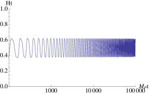
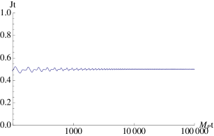
Figure 1: Time evolution of $H$ and $J$ for Example 1 is shown. In these figures, we have taken $V=\lambda\phi^{4}/4$, $\lambda=1$ and $f_{1}=0.2$. $H$ oscillates violently (Left) while $J$ does not (Right).

3.1.3 Particle production

Recalling that J is conserved during the inflaton oscillation, the oscillating part of the Hubble parameter is deduced from Eq. (3.7) as

$$\delta H \simeq-f_{1}\frac{\dot{\phi}}{2M_{P}}.$$ (3.15)

Then, from Eq. (2.26), the production rate is estimated as

$$\Gamma_{\phi\to\chi} \sim f_{1}^{2}\frac{m_{\rm{eff}}^{3}}{M_{P}^{2}},$$ (3.16)

where $m_{\rm eff}\sim\lambda^{1/2}\Phi^{n/2-1}$. This reproduces the result in [17, 16].

3.2 Example 2

As a second example, we consider

$$G_{2} =X-V(\phi),$$ (3.17)

$$G_{4} =\frac{1}{2}M_{P}^{2}+\frac{X}{2M^{2}}.$$ (3.18)

Note that this system is equivalent to

$$G_{2} =X-V(\phi),$$ (3.19)

$$G_{4} =\frac{1}{2}M_{P}^{2},$$ (3.20)

$$G_{5} =-\frac{\phi}{2M^{2}},$$ (3.21)

where $M_{P}$ is the reduced Planck mass and $M$ is some mass parameter.

3.2.1 Adiabatic invariant

The background action becomes

$$S_{G} =\int d^{4}x\;a^{3}\left[-3M_{P}^{2}H^{2}+\left(1+\frac{3H^{2}}{M^{2}}\right)\frac{\dot{\phi}^{2}}{2}-V\right],$$ (3.22)

after integration by parts. Therefore, $\mathcal{L}_{H}$ is given by

$$\mathcal{L}_{H}=-6M_{P}^{2}H\left(1-\frac{\dot{\phi}^{2}}{2M_{P}^{2}M^{2}}\right),$$ (3.23)

and the adiabatic invariant $J$ is given by

$$J =H\left(1-\frac{\dot{\phi}^{2}}{2M_{P}^{2}M^{2}}\right).$$ (3.24)

3.2.2 Expansion law

The background dynamics of this system is extensively studied in [13, 14], where it is shown that this system undergoes a nontrivial regime when $H^{2}/M^{2}\gg 1$. Let us focus on such a regime, when the Lagrangian is approximated as

$${\mathcal{L}} \simeq-3M_{P}^{2}H^{2}+\frac{3H^{2}}{M^{2}}\frac{\dot{\phi}^{2}}{2}-V.$$ (3.25)

Then, it can be decomposed as

$${\mathcal{L}} \simeq\frac{1}{2}H{\mathcal{L}}_{H}+\frac{1}{n}\phi{\mathcal{L}}_{\phi}.$$ (3.26)

Eqs. (2.21), (2.22) and (3.26) give

$$\left\langle{{\mathcal{L}}}\right\rangle =\frac{n+2}{2(n+1)}\left\langle{H{\mathcal{L}}_{H}}\right\rangle.$$ (3.27)

Substituting this into oscillation-averaged Eq. (2.16), one obtains the evolution equation for the adiabatic invariant $J$:

$$\dot{J}+\frac{3n}{2(n+1)}\left\langle{H}\right\rangle J=0.$$ (3.28)

From this equation one can derive

$$J \propto a^{-\frac{3n}{2(n+1)}}.$$ (3.29)

Now let us estimate the expansion law of the universe. Since $J\propto H(1-\dot{\phi}^{2}/2M_{P}^{2}M^{2})$, and the amplitude of $\dot{\phi}^{2}/M_{P}^{2}M^{2}$ is constant during the regime we consider, we have

$$\left\langle{H}\right\rangle\propto a^{-\frac{3n}{2(n+1)}},$$ (3.30)

and hence the expansion law is given by

$$\left\langle{H}\right\rangle =\frac{2(n+1)}{3n}\frac{1}{t}.$$ (3.31)

We plot the time dependence of $H$ and $J$ (multiplied by $t$) for $n=2$ in Fig. 2.

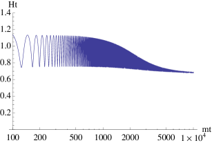
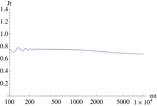
Figure 2: Time evolution of $H$ and $J$ for Example 2 is shown. In these figures, we have taken $V=m^{2}\phi^{2}/2$ and $m/M=10^{3}$. Left: Plot of $Ht$. $H$ violently oscillates in the non-minimal regime $H^{2}/M^{2}\gg 1$. The expansion law is $\left\langle{H}\right\rangle t=1$ for this regime, while it gradually approaches to the value with canonical kinetic term $2/3$ for $H^{2}/M^{2}\ll 1$. Right: Plot of $Jt$. It has a suppressed amplitude of oscillation compared to $Ht$.

3.2.3 Particle production

From Eq. (3.24), the oscillating part of the Hubble parameter is deduced as

$$\delta H \sim\frac{J\dot{\phi}^{2}}{M_{P}^{2}M^{2}}.$$ (3.32)

Thus, the decay rate of $\phi$ is estimated as

$$\Gamma_{\phi\to\chi}\sim\frac{m_{\rm eff}^{5}\Phi^{2}}{M_{P}^{4}M^{2}},$$ (3.33)

where we have taken $J\sim H$ as an order estimation, and $\Phi_{c}\sim H\Phi/M$. Also, $m_{\rm eff}\sim(M/H)\lambda^{1/2}\Phi^{n/2-1}$. This reproduces the result shown in [14] (for case B, where the non-minimal coupling effect is larger than the one that exists in the minimal setup).

3.3 Example 3

Finally let us consider the system

$$G_{2} =X-V(\phi),$$ (3.34)

$$G_{4} =\frac{1}{2}M_{P}^{2},$$ (3.35)

$$G_{5} =-\frac{\phi^{3}}{M^{4}},$$ (3.36)

where $M$ is some mass parameter.

3.3.1 Adiabatic invariant

The background action is

$$S_{G} =\int d^{4}x\;a^{3}\left[-3M_{P}^{2}H^{2}+\left(1+\frac{18H^{2}\phi^{2}}{M^{4}}\right)\frac{\dot{\phi}^{2}}{2}-V\right],$$ (3.37)

from which $\mathcal{L}_{H}$ is given by

$${\mathcal{L}}_{H} =-6M_{P}^{2}H\left(1-\frac{3\phi^{2}\dot{\phi}^{2}}{M_{P}^{2}M^{4}}\right).$$ (3.38)

Then, the adiabatic invariant $J$ is given by

$$J =H\left(1-\frac{3\phi^{2}\dot{\phi}^{2}}{M_{P}^{2}M^{4}}\right).$$ (3.39)

3.3.2 Expansion law

We focus on the regime when the non-minimal kinetic term takes a dominant role here. Then, the Lagrangian is approximated as

$${\mathcal{L}} \simeq-3M_{P}^{2}H^{2}+\frac{18H^{2}\phi^{2}}{M^{4}}\frac{\dot{\phi}^{2}}{2}-V,$$ (3.40)

and hence it is decomposed as

$${\mathcal{L}} \simeq\frac{1}{2}H{\mathcal{L}}_{H}+\frac{1}{n}\phi{\mathcal{L}}_{\phi}-\frac{1}{n}\dot{\phi}{\mathcal{L}}_{\dot{\phi}}.$$ (3.41)

Therefore, Eqs. (2.22), (2.21) and (3.41) give

$$\left\langle{\mathcal{L}}\right\rangle =\frac{n+4}{2(n+2)}\left\langle{H{\mathcal{L}}_{H}}\right\rangle.$$ (3.42)

Substituting this into Eq. (2.16), we get

$$\dot{J}+\frac{3n}{2(n+2)}\left\langle{H}\right\rangle J=0,$$ (3.43)

and thus

$$J \propto a^{-\frac{3n}{2(n+2)}}.$$ (3.44)

Since the absolute value of the second term in the parenthesis in Eq. (3.39) is less than $1/3$, as is guaranteed by the Friedmann equation, this term does not affect the power-law form of $J$. Thus,

$$\left\langle{H}\right\rangle \propto a^{-\frac{3n}{2(n+2)}}$$ (3.45)

and the expansion law of the universe is given by

$$\left\langle{H}\right\rangle =\frac{2(n+2)}{3n}\frac{1}{t}.$$ (3.46)

We plot $H$ and $J$ (multiplied by $t$) for $n=2$ in Fig. 3.

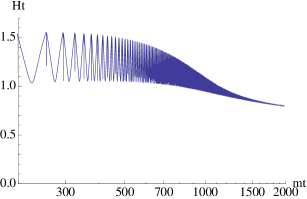
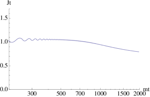
Figure 3: Time evolution of $H$ and $J$ for Example 3 is shown. In these figures, we have taken $V=m^{2}\phi^{2}/2$, $m/M_{P}=1$ and $M/M_{P}=10^{-5/2}$. Left: Plot of $Ht$. $H$ violently oscillates in the non-minimal regime $H^{2}\phi^{2}/M^{4}\gg 1$. The expansion law is $\left\langle{H}\right\rangle t=4/3$ for this regime, while it gradually approaches to the value with canonical kinetic term $2/3$ for $H^{2}\phi^{2}/M^{4}\ll 1$. Right: Plot of $Jt$. It has a suppressed amplitude of oscillation compared to $Ht$.

3.3.3 Particle production

From Eq. (3.39), the oscillating part of the Hubble parameter is

$$\delta H\sim J\frac{\phi^{2}\dot{\phi}^{2}}{M_{P}^{2}M^{4}},$$ (3.47)

and hence the decay rate is estimated as

$$\Gamma_{\phi\to\chi}\sim\frac{m_{\rm{eff}}^{5}\Phi^{4}}{M_{P}^{4}M^{4}},$$ (3.48)

where we have taken $J\sim H$ as an order estimation, and $\Phi_{c}\sim H\Phi^{2}/M^{2}$. Also, $m_{\rm eff}\sim(M^{2}/H\Phi)\lambda^{1/2}\Phi^{n/2-1}$.

4 Conclusion

In this paper, we study the generalized Galileon theories in the context of inflation, especially focusing on the inflaton oscillation regime. During this regime, in general, these models lead to violent oscillations of the Hubble parameter and the energy density of inflaton, and hence it would be desirable to construct an adiabatic quantity which evolves only with the time scale of $H^{-1}$. We have shown the existence of an adiabatic invariant $\dot{Q}={\mathcal{O}}(HQ)$ during this regime, and also shown an explicit method to construct this adiabatic invariant. To confirm our procedure, we have demonstrated that the proposed adiabatic invariant actually evolves with the time scale of $H^{-1}$ in several examples of generalized Galileon theories by numerical calculation. Such an invariant is useful in estimating the expansion law of the universe, and expressing the oscillation in the Hubble parameter in terms of the inflaton so as to estimate the amount of particle production via gravitational effects. Thus it may take crucial roles to predict the precise value of the spectral index.

We also emphasize that the analysis background dynamics is a first step to understand the actual phenomena in the oscillation regime. In a specific example of $G^{\mu\nu}\partial_{\mu}\phi\partial_{\nu}\phi$ model, the relation $|\dot{H}|\sim m_{\rm eff}H\gg H^{2}$ was crucial for the Laplacian instability [14]. Without correct understandings of the background dynamics, we cannot judge the phenomenological validity of various inflation models.

References

- [1] A. H. Guth, Phys. Rev. D 23, 347 (1981).
- [2] A. D. Linde, Phys. Lett. B 108, 389 (1982).
- [3] P. A. R. Ade et al. [Planck Collaboration], arXiv:1502.02114 [astro-ph.CO].
- [4] C. Deffayet, X. Gao, D. A. Steer and G. Zahariade, Phys. Rev. D 84, 064039 (2011) [arXiv:1103.3260 [hep-th]].
- [5] T. Kobayashi, M. Yamaguchi and J. Yokoyama, Prog. Theor. Phys. 126, 511 (2011) [arXiv:1105.5723 [hep-th]].
- [6] G. Aad et al. [ATLAS Collaboration], Phys. Lett. B 716, 1 (2012) [arXiv:1207.7214 [hep-ex]].
- [7] S. Chatrchyan et al. [CMS Collaboration], Phys. Lett. B 716, 30 (2012) [arXiv:1207.7235 [hep-ex]].
- [8] T. Futamase and K. i. Maeda, Phys. Rev. D 39, 399 (1989).
- [9] J. L. Cervantes-Cota and H. Dehnen, Nucl. Phys. B 442, 391 (1995) [astro-ph/9505069].
- [10] F. L. Bezrukov and M. Shaposhnikov, Phys. Lett. B 659, 703 (2008) [arXiv:0710.3755 [hep-th]].
- [11] C. Germani and A. Kehagias, Phys. Rev. Lett. 105, 011302 (2010) [arXiv:1003.2635 [hep-ph]].
- [12] F. Takahashi, Phys. Lett. B 693, 140 (2010) [arXiv:1006.2801 [hep-ph]].
- [13] R. Jinno, K. Mukaida and K. Nakayama, JCAP 1401, no. 01, 031 (2014) [arXiv:1309.6756 [astro-ph.CO]].
- [14] Y. Ema, R. Jinno, K. Mukaida and K. Nakayama, arXiv:1504.07119 [gr-qc].
- [15] J. Ohashi and S. Tsujikawa, JCAP 1210, 035 (2012) [arXiv:1207.4879 [gr-qc]].
- [16] Y. Ema, R. Jinno, K. Mukaida and K. Nakayama, arXiv:1502.02475 [hep-ph].
- [17] Y. Watanabe and E. Komatsu, Phys. Rev. D 75, 061301 (2007) [gr-qc/0612120].