Analysis of the expected density of internal equilibria in random evolutionary multi-player multi-strategy games

Abstract

In this paper, we study the distribution and behaviour of internal equilibria in a $d$-player $n$-strategy random evolutionary game where the game payoff matrix is generated from normal distributions. The study of this paper reveals and exploits interesting connections between evolutionary game theory and random polynomial theory. The main contributions of the paper are some qualitative and quantitative results on the expected density, $f_{n,d}$, and the expected number, $E(n,d)$, of (stable) internal equilibria. Firstly, we show that in multi-player two-strategy games, they behave asymptotically as $\sqrt{d-1}$ as $d$ is sufficiently large. Secondly, we prove that they are monotone functions of $d$. We also make a conjecture for games with more than two strategies. Thirdly, we provide numerical simulations for our analytical results and to support the conjecture. As consequences of our analysis, some qualitative and quantitative results on the distribution of zeros of a random Bernstein polynomial are also obtained.

1 Introduction

1.1 Motivation

Evolutionary game theory (EGT) has been proven to be a suitable mathematical framework to model biological and social evolution whenever the success of an individual depends on the presence or absence of other strategies maynard-smith:1982to ; hofbauer:1998mm ; nowak:2006bo . EGT was introduced in 1973 by Smith and Price SP73 as an application of classical game theory to biological contexts, and has since then been widely and successfully applied to various fields, not only biology itself, but also ecology, population genetics, and computational and social sciences maynard-smith:1982to ; axelrod:1984yo ; hofbauer:1998mm ; nowak:2006bo ; broom2013game ; Perc2010109 ; HanBook2013 ; gokhale2014evolutionary . In these contexts, the payoff obtained from game interactions is translated into reproductive fitness or social success hofbauer:1998mm ; nowak:2006bo . Those strategies that achieve higher fitness or are more successful, on average, are favored by natural selection, thereby increase in their frequency. Equilibrium points of such a dynamical system are the compositions of strategy frequencies where all the strategies have the same average fitness. Biologically, they predict the co-existence of different types in a population and the maintenance of polymorphism.

As in classical game theory with the dominant concept of Nash equilibrium mclennan2005asymptotic ; mclennan2005expected , the analysis of equilibrium points in random evolutionary games is of great importance because it allows one to describe various generic properties, such as the overall complexity of interactions and the average behaviours, in a dynamical system. Understanding properties of equilibrium points in a concrete system is important, but what if the system itself is not fixed or undefined? Analysis of random games is insightful for such scenarios. To this end, it is ambitious and desirable to answer the following general questions:

How are the equilibrium points distributed? How do they behave when the number of players and strategies change?

Mathematical analysis of equilibrium points and their stability in a general (multi-player multi-strategy) evolutionary game is challenging because one would need to cope with systems of multivariate polynomial equations of high degrees (see Section 2 for more details). Nevertheless, some recent attempts, both through numerical and analytical approaches, have been made. One approach is to study the probabilities of having a concrete number of equilibria, whether all equilibrium points or only the stable ones are counted, if the payoff entries follow a certain probability distribution gokhale:2010pn ; HTG12 . This approach has the advantage that these probabilities provide elaborate information on the distribution of the equilibria. However, it consists of sampling and solving of a system of multivariate polynomial equations; hence is restricted, even when using numerical simulations, to games of a small number of players and/or small number of strategies: it is known that it is impossible to (analytically) solve an algebraic equation of a degree greater than $5$ able:1824aa . Another possibility is to analyze the attainability of the patterns and the maximal number of evolutionarily stable strategies (ESS) maynard-smith:1982to ; hofbauer:1998mm , revealing to some extent the complexity of the interactions. This line of research has been paid much attention in evolutionary game theory and other biological fields such as population genetics karlin:1980aa ; vickers:1988aa ; haigh1989large ; broom:1993pa ; broom:1997aa ; altenberg:2010tp ; gokhale:2010pn ; HTG12 ; gokhale2014evolutionary . More recently, in DH15 , the authors investigate the expected number of internal equilibria in a multi-player multi-strategy random evolutionary game where the game payoff matrix is generated from normal distributions. By connecting EGT and random polynomial theory, they describe a computationally implementable formula of the mean number of internal equilibrium points for the general case, lower and upper bounds the multi-player two-strategy random games, and a close-form formula for the two-player multi-strategy games.

In this paper, we address the aforementioned questions, i.e., of analysing distributions and behaviours of the internal equilibria of a random evolutionary game, in an average manner. More specifically, we first analyse the expected density of internal equilibrium points, $f_{n,d}(\mathbf{t})$, i.e. the expected number of such equilibrium points per unit length at point $\mathbf{t}$, in a $d$-player $n$-strategy random evolutionary game where the game payoff matrix is generated from a normal distribution (for short, normal evolutionary games). Here the parameter $\mathbf{t}=(t_{i})_{i=1}^{n-1}$, with $t_{i}=\frac{x_{i}}{x_{n}}$, denotes the ratio of frequency of strategy $i\in\{1,\cdots,n-1\}$ to that of strategy $n$, respectively (more details in Section 2). In such a random game, we then analyse the expected number of internal equilibria, $E(n,d)$, and, as a result, characterize the expected number of internal stable equilibria, $\mathit{SE}(n,d)$. We obtain both quantitative (asymptotic formula) and qualitative (monotone properties) results of $f_{n,d}$ and $E(n,d)$, as functions of the ratios, $\mathbf{t}$, the number of players, $d$, and that of strategies, $n$.

To obtain these results, we develop further the connection between EGT and random polynomial theory explored in DH15 , and more importantly, establish appealing (previously unexplored) connections to the well-known classes of polynomials, the Bernstein polynomials and Legendre polynomials. In contrast to the direct approach used in gokhale:2010pn ; HTG12 , our approach avoids sampling and solving a system of multivariate polynomial equations, thereby enabling us to study games with large numbers of players and/or strategies.

We now summarise the main results of the present paper.

1.2 Main results

The main analytical results of the present paper can be summarized into three categories: asymptotic behaviour of the density function and the expected number of (stable) equilibria, a connection between the density function with the Legendre polynomials, and monotonic behaviour of the density function. In addition, we provide numerical results and illustration for the general games when both the numbers of players and strategies are large.

To precisely describe our main results, we introduce the following notation regarding asymptotic behaviour of two given functions $u$ and $v\colon[0,+\infty)\rightarrow[0,+\infty)$

$$u\lesssim v\quad\Leftrightarrow\quad\text{there exists a positive constant $C$ such that for all $k\in[0,+\infty)$}$$

$$\hskip 85.35826ptu(k)\leq Cv(k),$$

$$u\sim v\quad\Leftrightarrow\quad\text{it holds that}\quad u\lesssim v\quad\text{and}\quad v\lesssim u.$$

Note that throughout the paper we sometimes put arguments of a function as subscripts. For instance, the expected density of internal equilibrium points, $f_{n,d}(\mathbf{t})$, besides $\mathbf{t}$, is also analyzed as a function of $n$ and $d$. We will explicitly state which parameter(s) is being varied whenever necessary to avoid the confusion.

The main results of the present paper are the following. As described above, $f_{n,d}(\mathbf{t})$ denotes the expected number of internal equilibrium points per unit length at point $\mathbf{t}$, in a $d$-player $n$-strategy random evolutionary game where the game payoff matrix is generated from a normal distribution; $E(n,d)$ the expected number of internal equilibria; and $\mathit{SE}(n,d)$ the expected number of internal stable equilibria. The formal definitions of these three functions are given in Section 2.

1. In Theorem 3.1, we prove the following asymptotic behaviour of $f_{2,d}(t)$ for all $t>0$: $f_{2,d}(t)\sim\sqrt{d-1}$. We also prove that $f_{2,d}(t)$ is always bounded from above and $\lim_{d\rightarrow\infty}\frac{f_{2,d}(t)}{d-1}=0$.

2. In Theorem 3.2, we prove a novel upper bound for the expected number of multi-player two-strategy random games, $E(2,d)\lesssim\sqrt{d-1}\ln(d-1)$ and obtain its limiting behaviour: $\lim\limits_{d\rightarrow\infty}\frac{\ln E(2,d)}{\ln(d-1)}=\frac{1}{2}$. This upper bound is sharper than the one obtained in (DH15, , Theorem 2), which is, $E(2,d)\lesssim(d-1)^{\frac{3}{4}}$. These results lead to two important corollaries. First, we obtain a sharper bound for the expected number of stable equilibria, $\mathit{SE}(2,d)\lesssim\frac{1}{2}\sqrt{d-1}\ln(d-1)$, and the corresponding limit, $\lim\limits_{d\rightarrow\infty}\frac{\ln\mathit{SE}(2,d)}{\ln(d-1)}=\frac{1}{2}$, see Corollary 1. The second corollary, Corollary 2, is mathematically significant, in which we obtain lower and upper bounds and a limiting behaviour of the expected number of real zeros of a random Bernstein polynomial.

3. In Theorem 3.3, we establish an expression of $f_{2,d}(t)$ in terms of the Legendre polynomial and its derivative.

4. In Theorem 3.4, we express $f_{2,d}(t)$ in terms of the Legendre polynomials of two consecutive order.

5. In Theorem 3.5, we prove that $\frac{f_{2,d}(t)}{d}$ is a decreasing function of $d$ for any given $t>0$. Consequently, $\frac{E(2,d)}{d}$ and $\frac{\mathit{SE}(2,d)}{d}$ are decreasing functions of $d$.

6. In Proposition 2, we provide a condition for $f_{2,d}(t)$ being an increasing function of $d$ for any given $t>0$. We conjecture that this condition holds true and support it by numerical simulation.

7. In Theorem 4.1, we provide an upper bound for $f_{n,2}(\mathbf{t})$. We also make a conjecture for $f_{n,d}(\mathbf{t})$ and $E(n,d)$ in the general case ($n,d\geq 3$).

8. We offer numerical illustration for our main results in Section 4.2.

The density function $f_{n,d}(\mathbf{t})$ provides insightful information on the distribution of the internal equilibria: integrating $f_{n,d}(\mathbf{t})$ over any interval produces the expected number of real equilibria on that interval. In particular, the expected number of internal equilibria $E(n,d)$ is obtained by integrating $f_{n,d}(\mathbf{t})$ over the positive half of the space. Theorem 3.5 and Proposition 2, which are deduced from Theorems 3.3 and 3.4, are qualitative statements, which tell us how the expected number of internal equilibria per unit length $f_{2,d}$ in a $d$-player two-strategy game changes when the number of players $d$ increases. Theorem 3.1 quantifies its behaviour showing that $f_{2,d}$ is approximately (up to a constant factor) equal to $\sqrt{d-1}$. The function $h(d):=\sqrt{d-1}$, as seen in Theorem 3.1, certainly satisfies the properties that $h(d)$ increases but $\frac{h(d)}{d}$ decreases. Thus, it strengthens Theorem 3.5 and further supports Conjecture 1. Theorem 3.2 is also a quantitative statement which provides an asymptotic estimate for the expected number of internal (stable) equilibria.

Furthermore, it is important to note that the expected number of real zeros of a random polynomial has been extensively studied, dating back to 1932 with Block and Pólya’s seminal paper BP32 (see, for instance, EK95 for a nice exposition and TaoVu14 ; NNV15TMP for the most recent progress). Therefore, our results, in Theorems 3.2, 3.3 and 3.4, provide important, novel insights within the theory of random polynomials, but also reveal its intriguing connections and applications to EGT.

1.3 Organisation of the paper

The rest of the paper is structured as follows. In Section 2, we recall relevant details on EGT and random polynomial theory. Section 3 presents full analysis of the expected density function and the expect number of internal equilibria of a multi-player two-strategy game. The results on asymptotic behaviour and on the connection to Legendre polynomials and its applications are given in Sections 3.1 and 3.2, respectively. In Section 4, we provide analytical results for the two-player multi-strategy game and numerical simulations for the general case. Therein we also make a conjecture about an asymptotic formula for the density and the expected number of internal equilibria in the general case. In Section 5, we sum up and provide future perspectives. Finally, some detailed proofs are presented in the appendix.

2 Preliminaries: replicator dynamics and random polynomials

This section describes some relevant details of the EGT and random polynomial theory, to the extent we need here. Both are classical but the idea of using the latter to study the former has only been pointed out in our recent paper DH15 .

2.1 Replicator dynamics

The classical approach to evolutionary games is replicator dynamics taylor:1978wv ; zeeman:1980ze ; hofbauer:1998mm ; schuster:1983le ; nowak:2006bo , describing that whenever a strategy has a fitness larger than the average fitness of the population, it is expected to spread. Formally, let us consider an infinitely large population with $n$ strategies, numerated from 1 to $n$. They have frequencies $x_{i}$, $1\leq i\leq n$, respectively, satisfying that $0\leq x_{i}\leq 1$ and $\sum_{i=1}^{n}x_{i}=1$. The interaction of the individuals in the population is in randomly selected groups of $d$ participants, that is, they play and obtain their fitness from $d$-player games. We consider here symmetrical games (e.g. the public goods games and their generalizations hardin:1968mm ; hauert:2002in ; santos:2008xr ; pacheco:2009aa ; Han:2014tl ) in which the order of the participants is irrelevant. Let $\alpha^{i_{0}}_{i_{1},\ldots,i_{d-1}}$ be the payoff of the focal player, where $i_{0}$ ($1\leq i_{0}\leq n$) is the strategy of the focal player, and $i_{k}$ (with $1\leq i_{k}\leq n$ and $1\leq k\leq d-1$) be the strategy of the player in position $k$. These payoffs form a $(d-1)$-dimensional payoff matrix gokhale:2010pn , which satisfies (because of the game symmetry)

$$\alpha^{i_{0}}_{i_{1},\ldots,i_{d-1}}=\alpha^{i_{0}}_{i_{1}^{\prime},\ldots,i_{d-1}^{\prime}},$$ (1)

whenever $\{i_{1}^{\prime}\ldots,i_{d-1}^{\prime}\}$ is a permutation of $\{i_{1}\ldots,i_{d-1}\}$. This means that only the fraction of each strategy in the game matters.

The equilibrium points of the system are given by the points $(x_{1},\dots,x_{n})$ satisfying the condition that the fitnesses of all strategies are the same, which can be simplified to the following system of $n-1$ polynomials of degree $d-1$ DH15

$$\sum\limits_{\begin{subarray}{c}0\leq k_{1},...,k_{n}\leq d-1,\\ \sum^{n}\limits_{i=1}k_{i}=d-1\end{subarray}}\beta^{i}_{k_{1},...,k_{n-1}}\begin{pmatrix}d-1\\ k_{1},...,k_{n}\end{pmatrix}\prod\limits_{i=1}^{n}x_{i}^{k_{i}}=0\quad\text{ for }i=1,\dots,n-1,$$ (2)

where $\beta^{i}_{k_{1},...,k_{n-1}}:=\alpha^{i}_{k_{1},...,k_{n}}-\alpha^{n}_{k_{1},...,k_{n}}$, and $\begin{pmatrix}d-1\\ k_{1},\dots,k_{n}\end{pmatrix}=\frac{(d-1)!}{\prod\limits_{k=1}^{n}k_{i}!}$ are the multinomial coefficients. Assuming that all the payoff entries have the same probability distribution, then all $\beta^{i}_{k_{1},...,k_{n-1}}$, $i=1,\dots,n-1$, have symmetric distributions, i.e. with mean 0 HTG12 .

We focus on internal equilibrium points gokhale:2010pn ; HTG12 ; DH15 , i.e. $0<x_{i}<1$ for all $1\leq i\leq n-1$. Hence, by using the transformation $t_{i}=\frac{x_{i}}{x_{n}}$, with $0<t_{i}<+\infty$ and $1\leq i\leq n-1$, dividing the left hand side of the above equation by $x_{n}^{d-1}$ we obtain the following equation in terms of $(t_{1},\ldots,t_{n-1})$ that is equivalent to (2)

$$\sum\limits_{\begin{subarray}{c}0\leq k_{1},...,k_{n-1}\leq d-1,\\ \sum\limits^{n-1}_{i=1}k_{i}\leq d-1\end{subarray}}\beta^{i}_{k_{1},...,k_{n-1}}\begin{pmatrix}d-1\\ k_{1},...,k_{n}\end{pmatrix}\prod\limits_{i=1}^{n-1}t_{i}^{k_{i}}=0\quad\quad\text{ for }i=1,\dots,n-1.$$ (3)

Hence, finding an internal equilibria in a general $n$-strategy $d$-player random evolutionary game is equivalent to find a solution $(y_{1},\dots,y_{n-1})\in{\mathbb{R}_{+}}^{n-1}$ of the system of $(n-1)$ polynomials of degree $(d-1)$ in (3). This observation links the study of generic properties of equilibrium points in EGT to the theory of random polynomials.

2.2 Random polynomial theory

Suppose that all $\beta^{i}_{k_{1},...,k_{n-1}}$ are Gaussian distributions with mean $0$ and variance $1$, then for each $i$ ($1\leq i\leq n-1$), $A^{i}=\left\{\beta^{i}_{k_{1},...,k_{n-1}}\begin{pmatrix}d-1\\ k_{1},...,k_{n}\end{pmatrix}\right\}$ is a multivariate normal random vector with mean zero and covariance matrix $C$ given by

$$C=\mathrm{diag}\left(\begin{pmatrix}d-1\\ k_{1},...,k_{n}\end{pmatrix}^{2}\right)_{0\leq k_{i}\leq d-1,~{}\sum\limits_{i=1}^{n-1}k_{i}\leq d-1}.$$ (4)

The density function $f_{n,d}$ and the expected number $E(n,d)$ of equilibria can be computed explicitly. The lemma below is a direct consequence of (EK95, , Theorem 7.1) (see also (DH15, , Lemma 1)). For a clarity of notation, we use bold font to denote an element in high-dimensional Euclidean space such as $\mathbf{t}=(t_{1},\ldots,t_{n-1})\in\mathbb{R}^{n-1}$.

Lemma 1

Assume that $\{A^{i}\}_{1\leq i\leq n-1}$ are independent normal random vectors with mean zero and covariance matrix $C$ as in (4). The expected density of real zeros of Eq. (3) at a point $\mathbf{t}=(t_{1},\ldots,t_{n-1})$ is given by

$$f_{n,d}(\mathbf{t})=\pi^{-\frac{n}{2}}\Gamma\left(\frac{n}{2}\right)(\det L(\mathbf{t}))^{\frac{1}{2}},$$ (5)

where $\Gamma$ denotes the Gamma function and $L(\mathbf{t})$ the matrix with entries

$$L_{ij}(\mathbf{t}) =\frac{\partial^{2}}{\partial x_{i}y_{j}}(\log v(\mathbf{x})^{T}Cv(\mathbf{y}))\big{|}_{\mathbf{y}=\mathbf{x}=\mathbf{t}},$$

with

$$v(\mathbf{x})^{T}Cv(\mathbf{y})=\sum\limits_{\begin{subarray}{c}0\leq k_{1},...,k_{n-1}\leq d-1,\\ \sum\limits^{n-1}_{i=1}k_{i}\leq d-1\end{subarray}}\begin{pmatrix}d-1\\ k_{1},\ldots,k_{n}\end{pmatrix}^{2}\prod\limits_{i=1}^{n}x_{i}^{k_{i}}y_{i}^{k_{i}}.$$ (6)

As a consequence, the expected number of internal equilibria in a d-player n-strategy random game is determined by

$$E(n,d)=\int_{\mathbb{R}_{+}^{n-1}}f_{n,d}(\mathbf{t})\,d\mathbf{t}.$$ (7)

Note that the assumption in Lemma 1 is quite limited when applying to games with more than two strategies as in that case the independence of the $\alpha$ terms does not carry over into the independence of $\beta$ terms, see Remark 3 for a detailed discussion.

3 Multi-player two-strategy games

We provide mathematical analysis of the expected density function $f_{2,d}(t)$ and the expected number of equilibria $E(2,d)$ for a multi-player two-strategy game. Section 3.1 presents asymptotic behaviour. A connection to Legendre polynomials and its applications are given in 3.2. In Section 3.2, further applications of this connection to study monotonicity of the density function are explored.

3.1 Asymptotic behaviour of the density and the expected number of equilibria

In the case of multi-player two-strategy games ($n=2$), the system of polynomial equations in (2) becomes a univariate polynomial equation

$$\sum\limits_{k=0}^{d-1}\beta_{k}\begin{pmatrix}d-1\\ k\end{pmatrix}y^{k}\,(1-y)^{d-1-k}=0,$$ (8)

where $y$ is the fraction of strategy 1 (i.e., $1-y$ is that of strategy 2) and $\beta_{k}$ is the payoff to strategy 1 minus that to strategy 2 obtained in a $d$-player interaction with $k$ other participants using strategy 1. It is worth noticing that

$$b_{k,d}:=\begin{pmatrix}d-1\\ k\end{pmatrix}y^{k}\,(1-y)^{d-1-k},\quad k=0,\ldots,d-1,$$ (9)

is the Bernstein basis polynomials of degree $d-1$ Pet99 ; Kow06 . Therefore, the left-hand side of (8) is a random Bernstein polynomial of degree $d-1$. As a by-product of our analysis, see Theorem 3.2, we will later obtain an asymptotic formula of the expected real zeros of a random Bernstein polynomial.

Letting $t=\frac{y}{1-y}$ ($t\in{\mathbb{R}_{+}}$), Eq. (8) is simplified to

$$\sum\limits_{k=0}^{d-1}\beta_{k}\begin{pmatrix}d-1\\ k\end{pmatrix}t^{k}=0.$$ (10)

The expected density of real zeros of this equation at a point $t$ is $f_{2,d}(t)$. For simplicity of notation, from now on we write $f_{d}(t)$ instead of $f_{2,d}(t)$. We recall some properties of the density function $f_{d}(t)$ from (DH15, , Proposition 1) that will be used in the sequel.

Proposition 1 (DH15 )

The following properties hold

1. $f_{d}(0)=\frac{d-1}{\pi},\quad f_{d}(1)=\frac{d-1}{2\pi}\frac{1}{\sqrt{2d-3}}$.

2. $f_{d}(t)=\frac{1}{2\pi}\left[\frac{1}{t}G^{\prime}(t)\right]^{\frac{1}{2}}$, where

   $$G(t)=t\frac{\frac{d}{dt}M_{d}(t)}{M_{d}(t)}=t\frac{d}{dt}\log M_{d}(t)\quad\text{with}\quad M_{d}(t)=\sum\limits_{k=0}^{d-1}\begin{pmatrix}d-1\\ k\end{pmatrix}^{2}t^{2k}.$$ (11)

3. $f_{d}(t)$ has an alternative representation

   $$(2\pi f_{d}(t))^{2}=\sum\limits_{i=1}^{d-1}\frac{4r_{i}}{(t^{2}+r_{i})^{2}},$$ (12)

   where $r_{i}>0$ satisfies that $M_{d}(t)=\prod\limits_{i=1}^{d-1}(t^{2}+r_{i})$.

4. $t\mapsto f_{d}(t)$ is a decreasing function.

5. $f_{d}\left(\frac{1}{t}\right)=t^{2}f(t)$.

6. $E(2,d)=\int_{0}^{\infty}f_{d}(t)\,dt=2\int_{0}^{1}f_{d}(t)\,dt$.

Example 1

Below are some examples of $f_{d}(t)$, with $d=2,3$ and 4

$$f_{2}(t)=\frac{1}{\pi}\frac{1}{1+t^{2}},\quad f_{3}(t)=\frac{2}{\pi}\frac{\sqrt{1+t^{2}+t^{4}}}{1+4t^{2}+t^{4}},\quad f_{4}(t)=\frac{3}{\pi}\frac{\sqrt{1+4t^{2}+10t^{4}+4t^{6}+t^{8}}}{1+9t^{2}+9t^{4}+t^{6}}.$$

We recall that $t=\frac{y}{1-y}$, where $y$ is the fraction of strategy 1. We can write the density in terms of $y$ using the change of variable formula as follows.

$$f_{d}(t)\,dt=f_{d}\Big{(}\frac{y}{1-y}\Big{)}\frac{1}{(1-y)^{2}}\,dy.$$

Define $g_{d}(y)$ to be the density on the right-hand side of the above expression, i.e.,

$$g_{d}(y):=f_{d}\Big{(}\frac{y}{1-y}\Big{)}\frac{1}{(1-y)^{2}}.$$ (13)

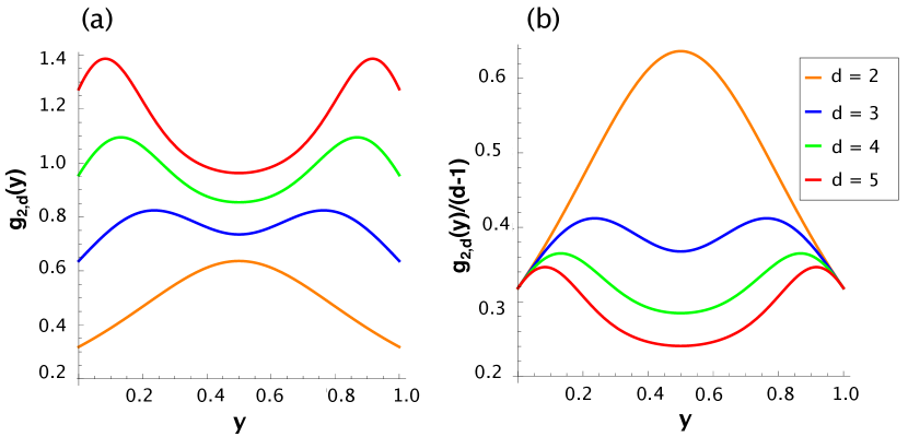
Figure 6: (a) Plot of $g_{2,d}(y)$ and (b) of $g_{2,d}(y)/(d-1)$ as functions of $y$ (note that $t=\frac{y}{1-y}$), for different values of $d$. We observe that both functions are symmetric about the line $y=1/2$, in accordance with Lemma 2. The first function increases with $d$ while the second one decreases. All the results were obtained numerically using Mathematica.

The following lemma is an interesting property of the density function $g_{d}$, which explains the symmetry of the strategies (swapping the index labels converts an equilibrium at $y$ to one at $1-y$). Numerical simulations in Section 4.2 further illustrate this property (see Figure 6).

Lemma 2

The function $y\mapsto g_{d}(y)$ is symmetric about the line $y=\frac{1}{2}$, i.e.,

$$g_{d}(y)=g_{d}(1-y).$$

Proof

We have

$$g_{d}(1-y)=f_{d}\Big{(}\frac{1-y}{y}\Big{)}\frac{1}{y^{2}}=f_{d}\Big{(}\frac{y}{1-y}\Big{)}\frac{y^{2}}{(1-y)^{2}}\frac{1}{y^{2}}=f_{d}\Big{(}\frac{y}{1-y}\Big{)}\frac{1}{(1-y)^{2}}=g_{d}(y),$$

where we have used the fifth property in Proposition 1 to obtain the second equality above.

The following theorem provides an upper bound and asymptotic behaviour for $f_{d}(t)$ and its scaling with respect to $d$.

Theorem 3.1 (Asymptotic behaviour of the density function)

The following statement holds

$$f_{d}(t)\leq\min\left\{\frac{\sqrt{d-1}}{2\pi\,t},\frac{d-1}{\pi}\right\}\quad\text{for}\quad t\geq 0.$$ (14)

As a consequence, for any given $t>0$

$$\frac{f_{d}(t)}{d-1}\leq\frac{1}{\pi},\quad\lim_{d\rightarrow\infty}\frac{f_{d}(t)}{d-1}=0,$$ (15)

and furthermore

$$f_{d}(t)\sim\sqrt{d-1}.$$ (16)

Proof

It follows from the first and the fourth properties in Proposition 1 that

$$f_{d}(t)\leq f_{d}(0)=\frac{d-1}{\pi}.$$ (17)

On the other hand, according to the third property in Proposition 1, we have

$$(2\pi f_{d}(t))^{2}=\sum_{i=1}^{d-1}\frac{4r_{i}}{(t^{2}+r_{i})^{2}}.$$

Since $(t^{2}+r_{i})^{2}\geq 4\,r_{i}t^{2}$, it follows that for any $t\neq 0$

$$(2\pi f_{d}(t))^{2}\leq\sum_{i=1}^{d-1}\frac{1}{t^{2}}=\frac{d-1}{t^{2}},$$

which is equivalent to $f_{d}(t)\leq\frac{\sqrt{d-1}}{2\pi\,t}$. Hence, the upper bound of $f_{d}(t)$ in (14) holds.

The upper bound and limit in (15) are obvious consequences of (14). It remains to prove the asymptotic behaviour of $f_{d}(t)$ as a function of $d$. Using (14) and the fourth property in Proposition 1, it follows that, for $0<t\leq 1$

$$\frac{d-1}{2\pi}\frac{1}{\sqrt{2d-3}}=f_{d}(1)\leq f_{d}(t)\leq\frac{\sqrt{d-1}}{2\pi\,t},$$

and for $t\geq 1$

$$\frac{1}{t^{2}}\frac{d-1}{2\pi}\frac{1}{\sqrt{2d-3}}=\frac{1}{t^{2}}f_{d}(1)\leq\frac{1}{t^{2}}f_{d}\left(\frac{1}{t}\right)=f_{d}(t)\leq f_{d}(1)=\frac{d-1}{2\pi}\frac{1}{\sqrt{2d-3}}.$$

From these estimates, we deduce that $f_{d}(t)\sim\sqrt{d-1}$ for any $t>0$.

We numerically illustrate Theorem 3.1 in Section 4.2, see Figures 1.

Theorem 3.2 (Asymptotic behaviour of $E(2,d)$)

It holds that

$$\sqrt{d-1}\lesssim E(2,d)\lesssim\sqrt{d-1}\ln(d-1).$$ (18)

Furthermore, we obtain the following asymptotic formula for $E(2,d)$

$$\lim\limits_{d\rightarrow\infty}\frac{\ln E(2,d)}{\ln(d-1)}=\frac{1}{2}.$$ (19)

We first provide a proof of this theorem. Then we discuss its implications for the expected number of stable equilibrium points in a random game and that of real zeros of a random Bernstein polynomial in Corollaries 1 and 2. A comparision with well-known results in the theory of random polynomials is given in Remark 1.

Proof

The lower bound was derived previously in (DH15, , Theorem 2). For the sake of completeness, we provide it again here. Using the sixth and the fourth properties in Proposition 1, we have $E(2,d)=2\int_{0}^{1}f_{d}(t)\,dt\geq 2\int_{0}^{1}f(1)\,dt=2f(1)=\frac{d-1}{\pi\sqrt{2d-3}}$. Therefore, $\sqrt{d-1}\lesssim E(2,d)$.

The underlying idea of the proof for the upper bound is to split the integral range in the formula of $E(2,d)$ into two intervals. The first one is from $0$ to $\alpha$, for some $\alpha\in(0,1)$; we then estimate $f_{d}(t)$ in this interval by $f_{d}(0)$. The second one is from $\alpha$ to $1$, which is estimated using the upper bound of $f_{d}(t)$ given in (14). The value of $\alpha$ will then be optimized.

$$E(2,d) =2\int_{0}^{1}f_{d}(t)\,dt=2\left[\int_{0}^{\alpha}f_{d}(t)\,dt+\int_{\alpha}^{1}f_{d}(t)\,dt\right]$$

$$\leq 2\left[\alpha f_{d}(0)+\frac{\sqrt{d-1}}{2\pi}\int_{\alpha}^{1}\frac{1}{t}\,dt\right]$$

$$=\frac{1}{\pi}\left[2(d-1)\,\alpha-\sqrt{d-1}\,\ln\alpha\right].$$ (20)

Let $h(\alpha)$ be the expression inside the square brackets in the right-hand side of (20). To obtain the optimal (i.e. smallest) upper bound, we minimize $h(\alpha)$ with respect to $\alpha$. The optimal value of $\alpha$ satisfies the following equation

$$\frac{d}{d\alpha}h(\alpha)=2(d-1)-\frac{\sqrt{d-1}}{\alpha}=0,$$

which leads to $\alpha=\frac{1}{2\sqrt{d-1}}$. Substituting this value into (20), we obtain

$$E(2,d)\leq\frac{\sqrt{d-1}}{\pi}\left(1+\ln 2+\frac{1}{2}\ln(d-1)\right).$$

It follows that $E(2,d)\lesssim\sqrt{d-1}\ln(d-1)$, which is (18).

We now prove (19). By taking logarithm in (18), we obtain

$$\frac{1}{2}\ln(d-1)\lesssim\ln E{(2,d)}\lesssim\frac{1}{2}\ln(d-1)+\ln\ln(d-1).$$

Therefore

$$\frac{1}{2}\lesssim\frac{\ln E(2,d)}{\ln(d-1)}\lesssim\frac{1}{2}+\frac{\ln\ln(d-1)}{\ln(d-1)}.$$ (21)

Since $\lim\limits_{d\rightarrow\infty}\frac{\ln\ln(d-1)}{\ln(d-1)}=0$, we achieve (19).

Theorem 3.2 has two interesting implications about the expected number of stable equilibrium points in a random game and that of real zeros of a random Bernstein polynomial.

Corollary 1

The expected number of stable equilibrium points in a random game with $d$ players and two strategies, $\mathit{SE}(2,d)$, satisfies

$$\frac{\sqrt{d-1}}{2}\lesssim\mathit{SE}(2,d)\lesssim\frac{1}{2}\sqrt{d-1}\ln(d-1),$$ (22)

and furthermore, satisfies the following limiting behaviour

$$\lim\limits_{d\rightarrow\infty}\frac{\ln\mathit{SE}(2,d)}{\ln(d-1)}=\frac{1}{2}.$$ (23)

Proof

From (HTG12, , Theorem 3), it is known that an equilibrium in a random game with two strategies and an arbitrary number of players, is stable with probability $1/2$. Thus, $\mathit{SE}(2,d)=\frac{E(2,d)}{2}$. Hence, the corollary is clearly followed from Theorem 3.2.

Corollary 2

The expected number of real zeros, $E_{\mathcal{B}}$, of a random Bernstein polynomial

$$\mathcal{B}(x)=\sum\limits_{k=0}^{d-1}\beta_{k}\begin{pmatrix}d-1\\ k\end{pmatrix}x^{k}\,(1-x)^{d-1-k},$$

where $\beta_{k}$ are independent standard normal distributions, satisfies

$$\sqrt{d-1}\lesssim E_{\mathcal{B}}\lesssim\sqrt{d-1}\ln(d-1),\quad\lim_{d\rightarrow\infty}\frac{\ln E_{\mathcal{B}}}{\ln(d-1)}=\frac{1}{2}.$$ (24)

Proof

As mentioned beneath (8), solving $\mathcal{B}(x)=0$ is equivalent to solving Eq. (10). It follows that $f_{d}(t)$ is the expected density of real zeros of $\mathcal{B}(x)$. Therefore, $E_{\mathcal{B}}$ given by

$$E_{\mathcal{B}}=\int_{-\infty}^{\infty}f_{d}(t)\,dt=2\int_{0}^{\infty}f_{d}(t)\,dt=2E(2,d).$$ (25)

Note that the second equality in (25) holds because $f_{d}(t)$ is even in $t$ due to (12). The asymptotic behaviour (24) of $E_{\mathcal{B}}$ is then followed directly from Theorem 3.2.

Remark 1

The study of the distribution and expected number of real zeros of a random polynomial is an active research field with a long history dating back to 1932 with Block and Pólya BP32 , see for instance EK95 for a nice exposition and TaoVu14 ; NNV15TMP for the most recent results and discussions. Consider a random polynomial of the type

$$\mathcal{P}_{d}(z)=\sum_{i=0}^{d-1}c_{i}\,\xi_{i}\,z^{i}.$$ (26)

The most well-known classes of polynomials studied extensively in the literature are: flat polynomials or Weyl polynomials for $c_{i}\colonequals\frac{1}{i!}$, elliptic polynomials (EP) or binomial polynomials for $c_{i}\colonequals\sqrt{\begin{pmatrix}d-1\\ i\end{pmatrix}}$ and Kac polynomials for $c_{i}\colonequals 1$. We emphasize the difference between the polynomial studied in this paper, i.e. the right-hand side of Eq. (10), with the elliptic polynomial: in our case $c_{i}=\begin{pmatrix}d-1\\ i\end{pmatrix}$ are binomial coefficients, not their square root as in the elliptic polynomial. In the former case, $v(x)^{T}Cv(y)=\sum_{i=1}^{d-1}\begin{pmatrix}d-1\\ i\end{pmatrix}x^{i}y^{i}=(1+xy)^{d-1}$, and as a result the density function and the expected number of real zeros have closed formula, see EK95

$$f_{EP}(t)=\frac{\sqrt{d-1}}{\pi(1+t^{2})},\quad E_{EP}=\sqrt{d-1}.$$

Our case is more challenging, because of the square in the coefficients,
$v(x)^{T}Cv(y)=\sum_{i=1}^{d-1}\begin{pmatrix}d-1\\ i\end{pmatrix}^{2}x^{i}y^{i}$ is no longer a generating function. Nevertheless, Theorem 3.2 shows that $E(2,d)$ still has interesting asymptotic behaviour as in (18) and (19).

3.2 Connections to Legendre polynomials and other qualitative properties

In this section, we first establish a connection between the expected density function $f_{d}$ and the well-known Legendre polynomials. Then using the connection and known properties of Legendre polynomials, we prove some qualitative properties of $f_{d}$ and the expected number of equilibria. The main results of this section can be summarised as follows.

1. Theorem 3.3 and Theorem 3.4 derive an expression for the expected density $f_{d}$ in terms of the Legendre polynomials.

2. Theorem 3.5 shows that $\frac{f_{d}(t)}{d-1}$ is an increasing function of $d$ for any given $t>0$.

3. Corollary 4 proves that $\frac{E(2,d)}{d-1}$ and $\frac{SE(2,d)}{d-1}$ are decreasing functions of $d$.

Technically, keys to these theorems are Lemma 3 that connects the Legendre polynomials $P_{d}$ to $M_{d+1}$ in (11), and Lemma 4 showing a reverse Turan’s inequality. These lemmas are of interest in their own right.

3.2.1 Legendre polynomials

We recall some relevant details on Legendre polynomials. Legendre polynomials, denoted by $P_{d}(x)$, are solutions to Legendre’s differential equation

$$\frac{d}{dx}\left[(1-x^{2})\frac{d}{dx}P_{d}(x)\right]+d(d+1)P_{d}(x)=0,$$ (27)

with initial data $P_{0}(x)=1,\ \ P_{1}(x)=x$. The following are some important properties of the Legendre polynomials that will be used in the sequel.

1. Explicit representation

   $$P_{d}(x)=\frac{1}{2^{d}}\sum_{i=0}^{d}\begin{pmatrix}d\\ i\end{pmatrix}^{2}(x-1)^{d-i}(x+1)^{i}.$$ (28)

2. Recursive relation

   $$(d+1)P_{d+1}(x)=(2d+1)xP_{d}(x)-dP_{d-1}(x).$$ (29)

3. First derivative relation

   $$\frac{x^{2}-1}{d}P_{d}^{\prime}(x)=xP_{d}(x)-P_{d-1}(x).$$ (30)

Example 2

The first few Legendre polynomials are

$$P_{0}(x)=1,\quad P_{1}(x)=x,\quad P_{2}(x)=\frac{1}{2}(3x^{2}-1),\quad P_{3}(x)=\frac{1}{2}(5x^{3}-3x),$$

$$\quad P_{4}(x)=\frac{1}{8}(35x^{4}-30x^{2}+3).$$

The Legendre polynomials were first introduced in 1782 by A. M. Legendre as the coefficients in the expansion of the Newtonian potential Legendre1785 . This expansion gives the gravitational potential associated to a point mass or the Coulomb potential associated to a point charge. In the course of time, Legendre polynomials have been widely used in Physics and Engineering. For instance, they occur when one solves Laplace’s equation (and related partial differential equations) in spherical coordinates Bayin06 .

Our approach reveals an appealing, and previously unexplored relationship between Legendre polynomials and evolutionary game theory. We explore this relationship and its applications in the next sections.

3.2.2 From Legendre polynomials to evolutionary games

The starting point of our analysis is the following relation between the polynomial $M_{d+1}(t)$ in (11) and the Legendre polynomial $P_{d}$.

Lemma 3

It holds that

$$M_{d+1}(t)=(1-t^{2})^{d}\,P_{d}\left(\frac{1+t^{2}}{1-t^{2}}\right).$$ (31)

Proof

See Appendix 6.1.

Note that traditionally in the Legendre polynomials, the arguments are in $[-1,1]$. In this paper, however, the arguments are not in this interval since $\big{|}\frac{1+t^{2}}{1-t^{2}}\big{|}\geq 1$. Legendre polynomials with arguments greater than unity have been used in the literature, for instance in (Cur03, , Chapter 2). We now establish a connection between the density $f_{d}(t)$ and the Legendre polynomials. According to the second property in Proposition 1, we have

$$f_{d+1}(t)=\frac{1}{2\pi}\left[\frac{1}{t}\left(t\frac{M_{d+1}^{\prime}(t)}{M_{d+1}(t)}\right)^{\prime}\right]^{\frac{1}{2}},$$ (32)

where ^′ denotes the derivative with respect to $t$. Using this formula and Lemma 3, we obtain the following expression of $f_{d+1}(t)$ in terms of $P_{d}(t)$ and its derivative.

Theorem 3.3 (Expression of the density in terms of the Legrendre polynomial and its derivative)

The following formula holds

$$(2\pi\,f_{d+1}(t))^{2}=\frac{4d^{2}}{(1-t^{2})^{2}}-\frac{16t^{2}}{(1-t^{2})^{4}}\left(\frac{P^{\prime}_{d}}{P_{d}}\right)^{2}\left(\frac{1+t^{2}}{1-t^{2}}\right)$$ (33)

Proof

See Appendix 6.2.

Corollary 3

As a direct consequence of (33), we obtain the following bound for $f_{2,d}(t)$.

$$f_{d}(t)\leq\frac{1}{\pi}\frac{d-1}{1-t^{2}}.$$ (34)

In comparison with the estimate (14) obtained in Theorem 3.1, this inequality is weaker for $t>0$ since it is of order $O(d-1)$. However, it does not blow up as $t$ approaches $0$.

We provide another expression of $f_{d+1}(t)$ in terms of two consecutive Legendre polynomials $P_{d-1}$ and $P_{d}$. In comparison with (33), this formula avoids the computations of the derivative of the Legendre polynomial $P_{d}$.

Theorem 3.4 (Expression of the density function in terms of two Legendre polynomials)

It holds that

$$(2\pi f_{d+1}(t))^{2}=\frac{4d^{2}}{(1-t^{2})^{2}}-\frac{d^{2}}{t^{2}}\left[\frac{1+t^{2}}{1-t^{2}}-\frac{P_{d-1}}{P_{d}}\left(\frac{1+t^{2}}{1-t^{2}}\right)\right]^{2}.$$ (35)

Proof

See Appendix 6.3

3.2.3 Monotonicity of the densities

Theorem 3.4 is crucial for the subsequent qualitative study of the density $f_{2,d}(t)$ for varying $d$.

Lemma 4

The following inequality holds for all $|x|\geq 1$

$$P_{d}(x)^{2}\leq P_{d+1}(x)P_{d-1}(x).$$ (36)

Proof

See Appendix 6.4.

Note that this inequality is the reverse of the Turán inequality Turan50 where the author considered the case $x\in[-1,1]$.

Theorem 3.5

For any given $t>0$, $\frac{f_{d}(t)}{d-1}$ is a decreasing function of $d$.

Proof

We need to prove that

$$\frac{f_{d+1}(t)}{d}\geq\frac{f_{d+2}(t)}{d+1}.$$

From (35), we have

$$4\pi^{2}\left(\frac{f_{d+1}(t)}{d}\right)^{2}=\frac{4}{(1-t^{2})^{2}}-\frac{1}{t^{2}}\left[\frac{1+t^{2}}{1-t^{2}}-\frac{P_{d-1}}{P_{d}}\left(\frac{1+t^{2}}{1-t^{2}}\right)\right]^{2}.$$ (37)

Assume that $x\geq 1$. Then $P_{d}(x)>0$ for all $d$ and from (29), we have

$$(d+1)P_{d+1}(x)\geq(2d+1)\,P_{d}(x)-d\,P_{d-1}(x),$$

which implies that

$$(d+1)(P_{d+1}(x)-P_{d}(x))\geq d(P_{d}(x)-P_{d-1}(x))\geq\cdots\geq 1(P_{1}(x)-P_{0}(x))=x-1\geq 0.$$

Therefore $P_{d+1}(x)\geq P_{d}(x)$ for all $x\geq 1$. We first consider the case $0\leq t<1$. From Lemma 4 for $x=\frac{1+t^{2}}{1-t^{2}}\geq 1$, we have

$$P_{d}^{2}\left(\frac{1+t^{2}}{1-t^{2}}\right)\leq P_{d-1}\left(\frac{1+t^{2}}{1-t^{2}}\right)P_{d+1}\left(\frac{1+t^{2}}{1-t^{2}}\right),$$

or equivalently

$$\frac{P_{d}}{P_{d+1}}\left(\frac{1+t^{2}}{1-t^{2}}\right)\leq\frac{P_{d-1}}{P_{d}}\left(\frac{1+t^{2}}{1-t^{2}}\right)\leq 1\leq\frac{1+t^{2}}{1-t^{2}}.$$

It follows that

$$\left[\frac{1+t^{2}}{1-t^{2}}-\frac{P_{d-1}}{P_{d}}\left(\frac{1+t^{2}}{1-t^{2}}\right)\right]^{2}\leq\left[\frac{1+t^{2}}{1-t^{2}}-\frac{P_{d}}{P_{d+1}}\left(\frac{1+t^{2}}{1-t^{2}}\right)\right]^{2}.$$

From this inequality and (37) as well as a similar formula for $f_{d+2}$, we obtain

$$\frac{f_{d+1}(t)}{d}\geq\frac{f_{d+2}(t)}{d+1},$$

which is the claimed property for the case $0\leq t<1$. The case $t\geq 1$ is then followed due to the relation $f_{d}(t)=\frac{1}{t^{2}}f_{d}\left(\frac{1}{t}\right)$.

Since $E(2,d)=\int_{0}^{\infty}f_{d}(t)\,dt$ and $\mathit{SE}(2,d)=\frac{E(2,d)}{2}$, the following statement is an obvious consequence of Theorem 3.5.

Corollary 4

$\frac{E(2,d)}{d-1}$ and $\frac{\mathit{SE}(2,d)}{d-1}$ are decreasing functions of $d$.

The following proposition is a necessary and sufficient condition, which is stated in terms of the Legendre polynomials, for $f_{d+1}(t)$ being increasing as a function of $d$.

Proposition 2

$f_{d+1}(t)$ is an increasing function of $d$ if and only if, for $x=\frac{1+t^{2}}{1-t^{2}}$

$$(d+1)^{2}[P^{2}_{d+1}(x)-P^{2}_{d}(x)]\cdot[P^{2}_{d+1}(x)+P^{2}_{d}(x)-2xP_{d+1}(x)P_{d}(x)]$$

$$\qquad+(2d+1)(x^{2}-1)P^{2}_{d}(x)P^{2}_{d+1}(x)\geq 0.$$ (38)

Furthermore, if

$$(2d+1)P_{d}^{4}\geq P_{d-1}^{2}\left[(2d-1)P_{d+1}^{2}+2P_{d}^{2}\right]$$ (39)

then (2) holds.

Proof

See Appendix 6.5.

We numerically verify the inequality (39) in Figure 2; however, it is unclear to us how to prove it rigorously. We also recall that it is shown in Theorem 3.1 that $f_{d}(t)$ behaves like $\sqrt{d-1}$, which is an increasing function of $d$, as $d$ is sufficiently large. Motivated by these observations, we make the following prediction.

Conjecture 1

For any given $t>0$, $f_{d}(t)$ is an increasing function of $d$.

We provide further numerical simulation to support this Conjecture by directly plotting $f_{d}(t)$ in Figure 1c.

Remark 2

We recall that in the case $n=2$, the variable $t$ is defined by $t=\frac{y}{1-y}$, where $y$ is the fraction of strategy $1$ and $1-y$ is that of strategy $2$. Equivalently, $y$ can be expressed in terms of $t$ as $y=\frac{t}{1+t}$. Hence one can also transform the statements of the theorem above (and later) in terms of $y$. As has been shown in the beginning of Section 2, the transformation from $y$ to $t$ has the advantage that it transforms a complex equation (Eq. (8)) to a univariate polynomial equation (Eq. (10)). This enables us to exploit many available results and techniques from the literature of random polynomial theory. Moreover, from the relationship between $f(t)$ and $g(y)$, it follows that all the monotonicity properties with respect to $d$ are reserved for $g_{2,d}$ (see a numerical illustration in Figure 6).

4 General Cases

In this section, first we prove an estimate for the density $f_{n,2}(\mathbf{t})$ similarly as in Theorem 3.1 for a two-player multi-strategy game. The expected number of internal equilibria in this case has been computed explicitly in (DH15, , Theorem 3). We then conjecture an asymptotic formula for the general case. Finally, we provide numerical simulations to support our conjectures, as well as the main results in the previous sections.

4.1 Two-player multi-strategy games

Theorem 4.1 (two-player multi-strategy games)

Assume that $\{A^{i}=(\beta_{j}^{i})_{j=1,\cdots,n-1};i=1,\ldots,n-1\}$ are independent random vectors, then it holds that

$$f_{n,2}(\mathbf{t})=\pi^{-\frac{n}{2}}\Gamma\left(\frac{n}{2}\right)\quad\text{if}~{}~{}t_{1}\cdots t_{n-1}=0\quad\text{and}$$ (40)

$$f_{n,2}(\mathbf{t})\leq\pi^{-\frac{n}{2}}\Gamma\left(\frac{n}{2}\right)\min\left\{1,\frac{1}{n^{\frac{n}{2}}\,t_{1}\,\cdots\,t_{n-1}}\right\}\quad\text{if}~{}~{}t_{1}\cdots t_{n-1}\neq 0.$$ (41)

As a consequence, for any $\mathbf{t}$ such that $t_{1}\cdots t_{n-1}\neq 0$

$$\lim_{n\rightarrow\infty}\frac{f_{n,2}(\mathbf{t})}{\pi^{-\frac{n}{2}}\Gamma\left(\frac{n}{2}\right)}=0.$$ (42)

Proof

According to (DH15, , Theorem 3)

$$f_{n,2}(\mathbf{t})=\pi^{-\frac{n}{2}}\Gamma\left(\frac{n}{2}\right)\frac{1}{\left(1+\sum\limits_{k=1}^{n-1}t_{k}^{2}\right)^{\frac{n}{2}}}.$$ (43)

The first assertion is then followed. Now suppose that $t_{1}\cdots t_{n-1}\neq 0$. By the Cauchy-Schwartz inequality, which states $\sum_{i=1}^{n}a_{n}\geq n(a_{1}\cdots a_{n})^{\frac{1}{n}}$ for $n$ all $n$ positive numbers $a_{1},\cdots,a_{n}$, we have

$$\left(1+\sum\limits_{k=1}^{n-1}t_{k}^{2}\right)^{\frac{n}{2}}\geq n^{\frac{n}{2}}\,t_{1}\,\cdots\,t_{n-1}.$$

Therefore

$$f_{n,2}(\mathbf{t})\leq\pi^{-\frac{n}{2}}\Gamma\left(\frac{n}{2}\right)\frac{1}{n^{\frac{n}{2}}\,t_{1}\,\cdots\,t_{n-1}}.$$

On the other hand, since $\left(1+\sum\limits_{k=1}^{n-1}t_{k}^{2}\right)^{\frac{n}{2}}\geq 1$, it follows that

$$f_{n,2}(\mathbf{t})\leq\pi^{-\frac{n}{2}}\Gamma\left(\frac{n}{2}\right).$$

Therefore, we obtain (41).

Note that the expected number of internal equilibria for a two-player multi-strategy game is given by (DH15, , Theorem 3)

$$E(n,2)=\frac{1}{2^{n-1}}.$$

Table 1: Expected number of internal equilibria for $n=3$ and different $d$, as generated from $E(3,d)$ and from averaging over $10^{6}$ random samples of the system of equation in 2. In all cases, results from random samplings are slightly smaller $E(3,d)$.

d	2	3	4	5
$E(3,d)$ from Theory	0.25	0.57	0.92	1.29
$E(3,d)$ from Random Sampling	0.249496	0.569169	0.910236	1.28898

Remark 3

In Theorem 4.1, we need an assumption that the random vectors $\{A^{i}=(\beta_{j}^{i})_{j=1,\cdots,n-1};i=1,\ldots,n-1\}$ are independent. Recalling from Section 2 that $\beta^{i}_{k_{1},...,k_{n-1}}=\alpha^{i}_{k_{1},...,k_{n}}-\alpha^{n}_{k_{1},...,k_{n}}$, where $\alpha^{i}_{i_{1},\ldots,i_{d-1}}$ is the payoff of the focal player, with $i$ ($1\leq i\leq n$) being the strategy of the focal player, and $i_{k}$ (with $1\leq i_{k}\leq n$ and $1\leq k\leq d-1$) is the strategy of the player in position $k$. The assumption clearly holds for $n=2$. For $n>2$, the assumption holds only under quite restrictive conditions such as $\alpha^{n}_{k_{1},...,k_{n}}$ is deterministic or $\alpha^{i}_{k_{1},...,k_{n}}$ are essentially identical. Note that the assumption is necessary to apply (EK95, , Theorem 7.1). Hence, to remove this assumption, one would need to generalize (EK95, , Theorem 7.1). This is difficult and is still an open problem Kos93 ; Kos01 . Nevertheless, since the system (3) has not been studied in the mathematical literature, it is interesting on its own to investigate the number of real zeros of this system under the assumption of independence of $\{A^{i}\}$. As such, the investigation not only provides new insights into the theory of zeros of systems of random polynomials but also gives important hint on the complexity of the game theoretical question, i.e. the number of expected number of equilibria. In Figure 7 and Table 1, we numerically compare the density function $g_{3,d}$ and the expected number of equilibria $E_{3,d}$ computed from the theory with the above assumption and from samplings without the assumption. We observe that $g_{3,d}$ have the same shape (behaviour) in both cases. In addition, the values of $E_{3,d}$ computed from samplings are slightly smaller than those computed from the theory.

We now make a conjecture for the expected density and expected number of equilibria in a general multi-player multi-strategy game.

Conjecture 2

In a multi-player multi-strategy game, it holds that

$$f_{n,d}\sim(d-1)^{\frac{n-1}{2}}\quad\text{and}\quad\lim_{d\rightarrow\infty}\frac{\ln E(n,d)}{\ln(d-1)}=\frac{n-1}{2}.$$ (44)

We envisage that even a stronger statement holds

$$E(n,d)\sim(d-1)^{\frac{n-1}{2}}.$$ (45)

This conjecture is motivated from Theorem 3.2 and a similar result for the system of multivariate elliptic polynomial as follows (see also Remark 1). Consider a system of $n-1$ random polynomials, each of the form

$$\sum\limits_{\begin{subarray}{c}0\leq k_{1},...,k_{n}\leq d-1,\\ \sum^{n}\limits_{i=1}k_{i}=d-1\end{subarray}}\beta_{k_{1},...,k_{n}}\sqrt{\begin{pmatrix}d-1\\ k_{1},...,k_{n}\end{pmatrix}}\prod\limits_{i=1}^{n}x_{i}^{k_{i}},$$ (46)

where the coefficients $\beta_{k_{1},...,k_{n}}$ are independent standard multivariate normal distribution. Then according to (EK95, , Section 7.2), the expected density and the expected number of real zeros are given by

$$f_{EP}(\mathbf{t})=\pi^{-\frac{n}{2}}\Gamma\left(\frac{n}{2}\right)\frac{(d-1)^{\frac{n-1}{2}}}{(1+\mathbf{t}\cdot\mathbf{t})^{\frac{n}{2}}},\quad E_{EP}=(d-1)^{\frac{n-1}{2}}.$$ (47)

These formula are direct consequences of Lemma 1 and the fact that $v(\mathbf{x})Cv(\mathbf{y})$ is a generating function, which generalises the univariate case

$$v(\mathbf{x})^{T}Cv(\mathbf{y})=\sum\limits_{\begin{subarray}{c}0\leq k_{1},...,k_{n}\leq d-1,\\ \sum^{n}\limits_{i=1}k_{i}=d-1\end{subarray}}\begin{pmatrix}d-1\\ k_{1},...,k_{n}\end{pmatrix}\prod\limits_{i=1}^{n}x^{k_{i}}y^{k_{i}}=(1+\mathbf{x}\cdot\mathbf{y})^{d-1}.$$

As mentioned in Remark 1, in our case $v(\mathbf{x})^{T}Cv(\mathbf{y})$ is no longer a generating function due to the square of the multinomial coefficients. Motivated by this and Theorem 3.2 for the univariate case, we expect that the conjecture holds for the general case (i.e. $d$-player $n$-strategy normal evolutionary games).

4.2 Numerical results

In this section, we provide numerical simulations for all the (main) results obtained in the previous sections. The following figures are plotted. In the following list, (1) to (4) are to illustrate and confirm the analytical results obtained in the previous sections. The others, from (5) to (10), are numerical simulations for the games with large $d$ and $n$. They also provide numerical support for Conjecture 2.

1. $f_{d}(t)$ and $f_{d}(t)/(d-1)$ as functions of $t$ for different values of $d$, see Figures 1a-b. Figure 1a illustrates the fourth property in Proposition 1 that $f_{d}(t)$ is increasing as a function of $t$. Figure 1b explains the scaling by showing that $f_{d}(t)/(d-1)$ is a bounded and decreasing function.

2. $f_{d}(t)$ and $f_{d}(t)/(d-1)$ as functions of $d$ for different values of $t$, see Figures 1c-d. These figures show that $f_{d}(t)$ increases with $d$ while $f_{d}(t)/(d-1)$ decreases, which are in agreement with Conjecture 1 and Theorem 3.5.

3. $f_{d}(x)$ and $f_{d}(x)/(d-1)$ as functions of the frequency $x$.

4. $\frac{\ln E(2,d)}{\ln(d-1)}$ as a function of $d$, see Figure 3a. This figure demonstrates Theorem 3.2 on the convergence of $\frac{\ln E(2,d)}{\ln(d-1)}$ to $1/2$ as $d$ tends to infinity.

5. $f_{3,d}(t_{1},t_{2})$ as a function of $\mathbf{t}=(t_{1},t_{2})$ for different values of $d$, see Figures 5a-c.

6. $f_{3,d}(t_{1},t_{2})$ as a function of $d$ for different values of $\mathbf{t}=(t_{1},t_{2})$, see Figure 4a.

7. $f_{4,d}(t_{1},t_{2},t_{3})$ as a function of $\mathbf{t}=(t_{1},t_{2},t_{3})$ for different values of $d$, see Figures 5d-f.

8. $f_{4,d}(t_{1},t_{2},t_{3})$ as a function of $d$ for different values of $\mathbf{t}=(t_{1},t_{2},t_{3})$, see Figure 4b.

9. $\frac{\ln E(3,d)}{\ln(d-1)}$ as a function of $d$, see Figure 3b.

10. $\frac{\ln E(4,d)}{\ln(d-1)}$ as a function of $d$, see Figure 3c.

In Figures 5, we provide numerical results of $f_{n,d}(\mathbf{t})$ for $n=3$ and $n=4$. We observe that the density function decreases with $t_{i}$ (namely, $t_{1}$ and $t_{2}$ for $n=3$, and $t_{1}$, $t_{2}$ and $t_{3}$ for $n=4$) and increases with $d$. We conjecture that for the general $d$-player $n$-strategy normal evolutionary game, the density function decreases with $t_{i}$ and increases with $d$.

Figures 3b and 3c support Conjecture 2. From these two figures, one also can see the complexity of the problem when $d$ increases. We are able to run simulations for $d$ up to $10000$ for $n=2$, up to $400$ for $n=3$ and only up to $20$ for $n=4$.

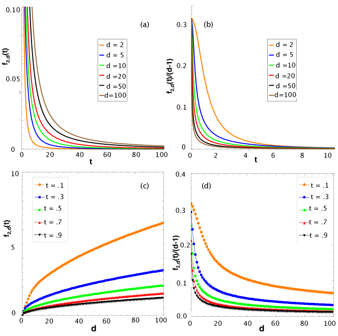
Figure 1: (a) Plot of $f_{2,d}(t)$ and (b) of $f_{2,d}(t)/(d-1)$ as functions of $t$, for different values of $d$. We observe that both functions decrease with $t$, which are in accordance with Proposition 1. The second function is bounded from above, having maximum at $t=0$, which agrees with Theorem 3.1. (c) Plot of $f_{2,d}(t)$ and (d) of $f_{2,d}(t)/(d-1)$ as functions of $d$, for different values of $t$. We observe that $f_{2,d}(t)$ increases with $d$, while $f_{2,d}(t)/(d-1)$ decreases, which are in agreement with Conjecture 1 and Theorem 3.5. All the results were obtained numerically using Mathematica.

Figure 2: Plot of $L_{d}(x):=(2d+1)P_{d}^{4}{\color[rgb]{1,0,0}-}P_{d-1}^{2}\left[(2d-1)P_{d+1}^{2}+2P_{d}^{2}\right]$ for different values of $d$. We observe that $L_{d}(x)$ is always non-negative, thereby supporting Conjecture 1, since the inequality $L_{d}(x)\geq 0$ is the sufficient condition for the conjecture, as shown in Proposition 2

.

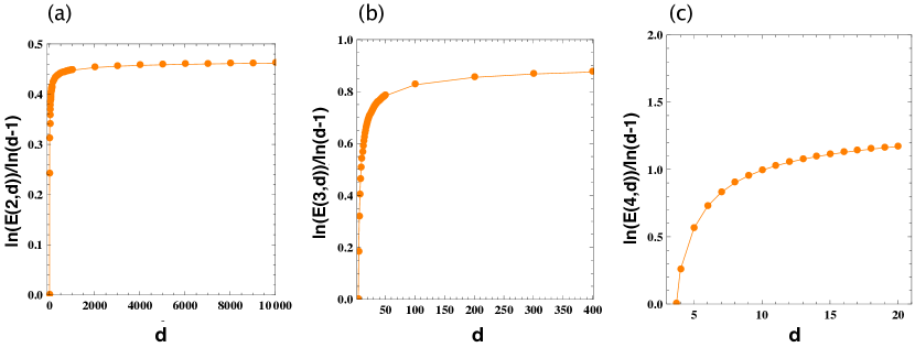
Figure 3: Plot of $\frac{\ln E(n,d)}{\ln(d-1)}$ as functions of $d$, (a) for $n=2$, (b) for $n=3$ and (c) for $n=4$. The results confirm the asymptotic behaviour for $n=2$ as described in Theorem 3.2, and clearly support Conjecture 2 for the general case. All the results were obtained numerically using Mathematica.

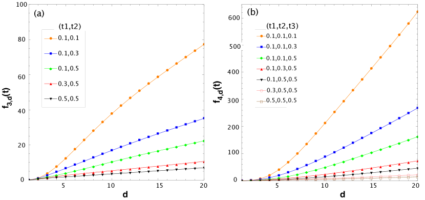
Figure 4: Plot of (a) $f_{3,d}(t_{1},t_{2})$ for different values of $(t_{1},t_{2})$ and (b) $f_{4,d}(t_{1},t_{2})$ for different values of $(t_{1},t_{2},t_{3})$, both as a function of $d$. We observe that the functions increase with $d$ while decrease with $t_{i}$, with $i=1,2$ in panel (a) and $i=1,2,3$ in panel (b). All the results were obtained numerically using Mathematica.

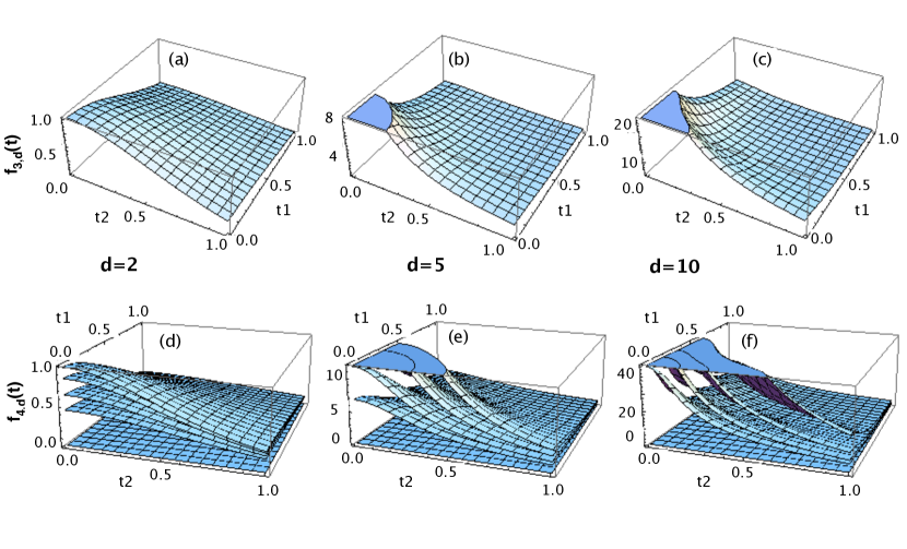
Figure 5: Plot of (a-c) $f_{3,d}(t_{1},t_{2})$ as a function of $(t_{1},t_{2})$; and (d-f) $f_{4,d}(t_{1},t_{2})$ as a function of $(t_{1},t_{2})$, for different values of $t_{3}$. We observe that both functions increase with $d$ while decrease with $t_{i}$, with $i=1,2$ in panels (a)-(c) and $i=1,2,3$ in panels (d)-(f). In panels (a) and (d), $d=2$; in panels (b) and (e), $d=5$; in panels (c) and (f), $d=10$. In panels (d)-(f), the surfaces, from bottom to top, correspond to $t_{3}=0.1,\ 0.3,\ 0.5,\ 0.7$ and $10$, respectively. All the results were obtained numerically using Mathematica.

Figure 7: (Top row) Plot of the density function $g_{3,d}(y_{1},y_{2})$ for different values of $d$ (here $y_{1}$ and $y_{2}$ are fractions of strategy 1 and 2, respectively, and $1-y_{1}-y_{2}$ is that of the third strategy). (Bottom row) Probability histograms plots of results from solving the system of equations 2 with $n=3$ and for different $d$, where the payoff entries $\alpha$’s are (independently) sampled from Gaussian distribution with mean 0 and standard deviation of 0.5 ($10^{6}$ samples in total). The probability histograms have similar shapes to $g_{3,d}(y_{1},y_{2})$ (see also Table 1). All the results were obtained numerically using Mathematica.

5 Discussion and outlook

How do equilibrium points in a general evolutionary game distribute if the payoff matrix entries are randomly drawn, and furthermore, how do they behave when the numbers of players and strategies change? To address these important questions regarding generic properties of general evolutionary games, we have analyzed here the density function, $f_{n,d}$, and the expected number of (stable) equilibrium points, $E(n,d)$ (respectively, $\mathit{SE}(n,d)$), in a normal $d$-player $n$-strategy evolutionary game. We have shown, analytically and using numerical simulations, that $f_{2,d}(t)$ monotonically decreases with $t$ while it increases with $d$. The latter implies that, as the number of players in the game increases, it is more likely to see an equilibrium at a given point $t$. We also proved that its scaling with respect to the number of players in a game $d$, $\frac{f_{2,d}(t)}{d}$, decreases with $d$. More interestingly, we proved that this density function asymptotically behaves in the same manner as $\sqrt{d-1}$ at any given $t$ (i.e. regardless of the equilibrium point). Similar monotonicity behaviors of the density function were observed numerically for games with larger numbers of strategies $n$. Additionally, we proved an upper bound for two-player game with an arbitrary number of strategies, $n$. Briefly, our analysis of the expected density of equilibrium points has offered clear and fresh understanding about equilibrium distribution. Related to this distribution analysis, there have been some works analyzing patterns of ESSs and their attainability in concrete games, i.e. with a fixed payoff matrix vickers1988patterns ; cannings1988patterns ; broom1994sequential . Differently, our analysis addresses distribution of the general equilibrium points, and for generic games. Note also that those works dealt with two-player games while we address here the general case (i.e. with arbitrary $d$).

Regarding the expected numbers of internal (stable) equilibrium points, first of all, as a result of the described monotonicity properties of the density function, we established analytically that $E(2,d)$ and $\mathit{SE}(2,d)$ increase with $d$ while their scaled forms, $\frac{E(2,d)}{d}$ and $\frac{\mathit{SE}(2,d)}{d}$, decrease with $d$. Next, we proved a new upper bounds for $n=2$, with arbitrary $d$: $E(2,d)\lesssim\sqrt{d-1}\ln(d-1)$. This upper bound is sharper than the one described in DH15 (which is also the only known one, to the best of our knowledge). As a consequence, a sharper upper bound for the number of expected number of stable equilibria can be established: $\mathit{SE}(2,d)\lesssim\frac{1}{2}\sqrt{d-1}\ln(d-1)$. More importantly, that allowed us to derive close-form limiting behaviors for such numbers: $\lim\limits_{d\rightarrow\infty}\frac{\ln E(2,d)}{\ln(d-1)}=\frac{1}{2}$ and $\lim\limits_{d\rightarrow\infty}\frac{\ln\mathit{SE}(2,d)}{\ln(d-1)}=\frac{1}{2}$. As such, apart from the mathematical elegance of our results, the analysis here has significantly improved existing results on the studies of random evolutionary game theory DH15 ; HTG12 ; gokhale:2010pn . Moreover, generalizing these formulas for the general case, i.e. when the number of strategies $n$ is also arbitrary, our conjecture that, $\lim\limits_{d\rightarrow\infty}\frac{\ln E(n,d)}{\ln(d-1)}=\frac{n-1}{2}$, is nicely corroborated by numerical simulations. Related to this analysis, there have been some works analyzing ESS in random evolutionary games haigh1988distribution ; kontogiannis2009support ; hart2008evolutionarily . In both haigh1988distribution and kontogiannis2009support , the authors focused on the asymptotic behaviour of ESS with large support sizes, i.e. considering also equilibrium points which are not internal, in random pairwise games. In a similar context, in hart2008evolutionarily , the authors studied ESS but with support size of two, showing the asymptotic behaviors of such ESS when the number of strategies varies. Differently from all these works (which dealt exclusively with two-player interactions), our analysis copes with multi-player games. Hence, our results have led to further understanding with respect to the asymptotic behaviour of the expected number of stable equilibria for multi-player random games.

Last but not least, as the density functions we analyzed here are closely related to Legendre polynomials, and actually, they are of the same form as the Bernstein polynomials, we have made a clear contribution to the longstanding theory of random polynomials BP32 ; EK95 ; TaoVu14 ; NNV15TMP (see again discussion in introduction). We have derived asymptotic behaviors for the expected real zeros $E_{\mathcal{B}}$ of a random Bernstein polynomial, which, to our knowledge, had not been provided before. Note that the asymptotic behaviors and close forms of the expected real zeros of some other well-known polynomials have been derived by other authors. For instance, the Weyl polynomials for $a_{i}\colonequals\frac{1}{i!}$; the elliptic polynomials or binomial polynomials with $a_{i}\colonequals\sqrt{\begin{pmatrix}d-1\\ i\end{pmatrix}}$; and Kac polynomials with $a_{i}\colonequals 1$. The difference between the polynomial studied here (i.e. Bernstein) with the elliptic case: $a_{i}=\begin{pmatrix}d-1\\ i\end{pmatrix}$ are binomial coefficients, not their square root. In the elliptic case, $v(x)^{T}Cv(y)=\sum_{i=1}^{d-1}\begin{pmatrix}d-1\\ i\end{pmatrix}x^{i}y^{i}=(1+xy)^{d-1}$, and as a result, $E(2,d)=\sqrt{d-1}$; While in our case, because of the square in the coefficients, $v(x)^{T}Cv(y)=\sum_{i=1}^{d-1}\begin{pmatrix}d-1\\ i\end{pmatrix}^{2}x^{i}y^{i}$, is no longer a generating function. Indeed, due to this difficulty, the analysis of the Bernstein polynomials is still rather limited, see for instance armentano2009note for a detailed discussion.

In short, our analysis has provided new understanding about the generic behaviors of equilibrium points in a general evolutionary game, namely, how they distribute and change in number when the number of players and that of the strategies in the game, are magnified.

6 Appendix

Detailed proofs of some lemmas and theorems in the previous sections are presented in this appendix.

6.1 Proof of Lemma 3

This relation has appeared in (GKP94, , Exercise 101, Chapter 5). For the readers’ convenience, we provide a proof here.

Proof (Proof of Lemma 3)

Let $x=\frac{1+q}{1-q}$, from (28) we have

$$P_{d}\left(\frac{1+q}{1-q}\right) =\frac{1}{2^{d}}\sum_{i=0}^{d}\begin{pmatrix}d\\ i\end{pmatrix}^{2}\left(\frac{1+q}{1-q}-1\right)^{d-i}\left(\frac{1+q}{1-q}+1\right)^{i}$$

$$=\frac{1}{2^{d}}\sum_{i=0}^{d}\begin{pmatrix}d\\ i\end{pmatrix}^{2}\left(\frac{2q}{1-q}\right)^{d-i}\left(\frac{2}{1-q}\right)^{i}$$

$$=\frac{1}{(1-q)^{d}}\sum_{i=0}^{d}\begin{pmatrix}d\\ i\end{pmatrix}^{2}q^{d-i}$$

$$=\frac{1}{(1-q)^{d}}\sum_{i=0}^{d}\begin{pmatrix}d\\ i\end{pmatrix}^{2}q^{i}.$$

Therefore,

$$\sum_{i=0}^{d}\begin{pmatrix}d\\ i\end{pmatrix}^{2}q^{i}=(1-q)^{d}P_{d}\left(\frac{1+q}{1-q}\right).$$

By taking $q=t^{2}$, we obtain (31).

6.2 Proof of Theorem 3.3

Proof (Proof of Theorem 3.3 )

By taking the derivative of both sides in (31), we obtain

$$M_{d+1}^{\prime}(t) =-2\,t\,d\,(1-t^{2})^{d-1}P_{d}\left(\frac{1+t^{2}}{1-t^{2}}\right)+4t(1-t^{2})^{d-2}P_{d}^{\prime}\left(\frac{1+t^{2}}{1-t^{2}}\right)$$

$$=-2\,t\,d\,\frac{M_{d+1}(t)}{1-t^{2}}+4t(1-t^{2})^{d-2}P_{d}^{\prime}\left(\frac{1+t^{2}}{1-t^{2}}\right).$$

It follows that

$$\frac{M_{d+1}^{\prime}(t)}{M_{d+1}(t)}=\frac{-2\,t\,d}{1-t^{2}}+\frac{4t}{(1-t^{2})^{2}}\frac{P_{d}^{\prime}}{P_{d}}\left(\frac{1+t^{2}}{1-t^{2}}\right).$$

Now we compute the expression inside the square-root of the right-hand side of (32). We have

$$t\frac{M_{d+1}^{\prime}(t)}{M_{d+1}(t)}=\frac{-2\,t^{2}\,d}{1-t^{2}}+\frac{4t^{2}}{(1-t^{2})^{2}}\frac{P_{d}^{\prime}}{P_{d}}\left(\frac{1+t^{2}}{1-t^{2}}\right),$$

and

$$\left(t\frac{M_{d+1}^{\prime}(t)}{M_{d+1}(t)}\right)^{\prime}=-\frac{4\,t\,d}{(1-t^{2})^{2}}+\frac{8t(1+t^{2})}{(1-t^{2})^{3}}\frac{P_{d}^{\prime}}{P_{d}}\left(\frac{1+t^{2}}{1-t^{2}}\right)+\frac{16t^{3}}{(1-t^{2})^{4}}\frac{P_{d}^{\prime\prime}\,P_{d}-(P^{\prime}_{d})^{2}}{P_{d}^{2}}\left(\frac{1+t^{2}}{1-t^{2}}\right).$$

Substituting this expression into (33), we get

$$(2\pi f_{d+1}(t))^{2}=-\frac{4\,d}{(1-t^{2})^{2}}+\frac{8(1+t^{2})}{(1-t^{2})^{3}}\frac{P_{d}^{\prime}}{P_{d}}\left(\frac{1+t^{2}}{1-t^{2}}\right)+\frac{16t^{2}}{(1-t^{2})^{4}}\frac{P_{d}^{\prime\prime}\,P_{d}-(P^{\prime}_{d})^{2}}{P_{d}^{2}}\left(\frac{1+t^{2}}{1-t^{2}}\right).$$ (48)

According to (27), the Legendre polynomial $P_{d}$ satisfies the following equation for all $x\in\mathbf{R}$

$$-2xP_{d}^{\prime}(x)+(1-x^{2})P^{\prime\prime}_{d}(x)=-d(d+1)P_{d}(x).$$

As a consequence, we obtain

$$\frac{P^{\prime\prime}_{d}(x)}{P_{d}(x)}=\frac{1}{1-x^{2}}\left(2x\frac{P_{d}^{\prime}(x)}{P_{d}(x)}-d(d+1)\right).$$

Substituting this expression into (48) with $x=\frac{1+t^{2}}{1-t^{2}}$, we get

$$(2\pi f_{d+1}(t))^{2} =-\frac{4\,d}{(1-t^{2})^{2}}+\frac{8(1+t^{2})}{(1-t^{2})^{3}}\frac{P_{d}^{\prime}}{P_{d}}\left(\frac{1+t^{2}}{1-t^{2}}\right)$$

$$\qquad+\frac{16t^{2}}{(1-t^{2})^{4}}\left\{\frac{1}{1-\left(\frac{1+t^{2}}{1-t^{2}}\right)^{2}}\left[2\frac{1+t^{2}}{1-t^{2}}\frac{P_{d}^{\prime}}{P_{d}}\left(\frac{1+t^{2}}{1-t^{2}}\right)-d(d+1)\right]-\left(\frac{P_{d}^{\prime}}{P_{d}}\right)^{2}\left(\frac{1+t^{2}}{1-t^{2}}\right)\right\}$$

$$=\frac{4d^{2}}{(1-t^{2})^{2}}-\frac{16t^{2}}{(1-t^{2})^{4}}\left(\frac{P_{d}^{\prime}}{P_{d}}\right)^{2}\left(\frac{1+t^{2}}{1-t^{2}}\right),$$

which is the claimed relation (33).

6.3 Proof of Theorem 3.4

Proof (Proof of Theorem 3.4)

Using the following relation of the Legendre polynomials for all $x\in\mathbf{R}$

$$P_{d}^{\prime}(x)=\frac{d}{x^{2}-1}\left(xP_{d}(x)-P_{d-1}(x)\right),$$

we get

$$\frac{P_{d}^{\prime}(x)}{P_{d}(x)}=\frac{d}{x^{2}-1}\left(x-\frac{P_{d-1}(x)}{P_{d}(x)}\right).$$ (49)

In particular, taking $x=\frac{1+t^{2}}{1-t^{2}}$, we obtain

$$\frac{P^{\prime}_{d}}{P_{d}}\left(\frac{1+t^{2}}{1-t^{2}}\right) =\frac{d}{\left(\frac{1+t^{2}}{1-t^{2}}\right)^{2}-1}\left[\frac{1+t^{2}}{1-t^{2}}-\frac{P_{d-1}}{P_{d}}\left(\frac{1+t^{2}}{1-t^{2}}\right)\right]$$

$$=\frac{d(1-t^{2})^{2}}{4t^{2}}\left[\frac{1+t^{2}}{1-t^{2}}-\frac{P_{d-1}}{P_{d}}\left(\frac{1+t^{2}}{1-t^{2}}\right)\right].$$

Substituting this expression into (33), we achieve

$$(2\pi f_{d+1}(t))^{2}=\frac{4d^{2}}{(1-t^{2})^{2}}-\frac{d^{2}}{t^{2}}\left[\frac{1+t^{2}}{1-t^{2}}-\frac{P_{d-1}}{P_{d}}\left(\frac{1+t^{2}}{1-t^{2}}\right)\right]^{2},$$

which is (35).

6.4 Proof of Lemma 4

Proof (Proof of Lemma 4)

This lemma follows directly from constantinescu2005inequality (Theorem 2.1) where the authors proved that

$$P_{d}(x)^{2}-P_{d+1}(x)P_{d-1}(x)=\frac{1-x^{2}}{d(d+1)}\left(\sum_{i=1}^{d}\frac{1}{i}+\sum_{i=1}^{d-1}\frac{1}{i+1}\sum_{j=1}^{i}(2j+1)P_{j}^{2}(x)\right),$$

which is negative for all $|x|\geq 1$.

6.5 Proof of Proposition 2

Proof (Proof of Proposition 2)

We will prove that

$$f^{2}_{d+2}(t)-f^{2}_{d+1}(t)\geq 0\quad\Longleftrightarrow\quad\eqref{eq: condition for fd increase}.$$ (50)

From (35), we have

$$4\pi^{2}(f^{2}_{d+2}(t)-f^{2}_{d+1}(t)) =\frac{4(d+1)^{2}}{(1-t^{2})^{2}}-\frac{(d+1)^{2}}{t^{2}}\left[\frac{1+t^{2}}{1-t^{2}}-\frac{P_{d}}{P_{d+1}}\left(\frac{1+t^{2}}{1-t^{2}}\right)\right]^{2}$$

$$\qquad-\frac{4d^{2}}{(1-t^{2})^{2}}+\frac{d^{2}}{t^{2}}\left[\frac{1+t^{2}}{1-t^{2}}-\frac{P_{d-1}}{P_{d}}\left(\frac{1+t^{2}}{1-t^{2}}\right)\right]^{2}$$

$$=\frac{4(2d+1)}{(1-t^{2})^{2}}-\frac{1}{t^{2}}\left[\frac{1+t^{2}}{1-t^{2}}-\frac{(d+1)P_{d}^{2}-dP_{d-1}P_{d+1}}{P_{d}P_{d+1}}\left(\frac{1+t^{2}}{1-t^{2}}\right)\right]\times$$

$$\qquad\left[(2d+1)\frac{1+t^{2}}{1-t^{2}}-\frac{(d+1)P_{d}^{2}+dP_{d-1}P_{d+1}}{P_{d}P_{d+1}}\left(\frac{1+t^{2}}{1-t^{2}}\right)\right].$$

Therefore $f_{d}(t)$ is increasing as a function of $d$ if and only if

$$\left[\frac{1+t^{2}}{1-t^{2}}-\frac{(d+1)P_{d}^{2}-dP_{d-1}P_{d+1}}{P_{d}P_{d+1}}\left(\frac{1+t^{2}}{1-t^{2}}\right)\right]\times\left[(2d+1)\frac{1+t^{2}}{1-t^{2}}-\frac{(d+1)P_{d}^{2}+dP_{d-1}P_{d+1}}{P_{d}P_{d+1}}\left(\frac{1+t^{2}}{1-t^{2}}\right)\right]$$

$$\qquad\leq\frac{4(2d+1)t^{2}}{(1-t^{2})^{2}}.$$

We re-write the expression above using the variable $x$, using the relation $x^{2}-1=\frac{4t^{2}}{(1-t^{2})^{2}}$, as follows

$$\left[x-\frac{(d+1)P_{d}^{2}-dP_{d-1}P_{d+1}}{P_{d}P_{d+1}}(x)\right]\times\left[(2d+1)x-\frac{(d+1)P_{d}^{2}+dP_{d-1}P_{d+1}}{P_{d}P_{d+1}}(x)\right]\leq(2d+1)(x^{2}-1).$$ (51)

We now simplify this expression using the recursion relation of the Legendre polynomials, i.e. $dP_{d-1}=(2d+1)xP_{d}-(d+1)P_{d+1}$. Namely, we have

$$xP_{d}P_{d+1}-(d+1)P_{d}^{2}+dP_{d-1}P_{d+1} =xP_{d}P_{d+1}-(d+1)P_{d}^{2}+[(2d+1)xP_{d}-(d+1)P_{d+1}]P_{d+1}$$

$$=(d+1)[-P_{d}^{2}-P_{d+1}^{2}+2xP_{d}P_{d+1}]$$

and

$$(2d+1)xP_{d}P_{d+1}-(d+1)P_{d}^{2}-dP_{d-1}P_{d+1}$$

$$\qquad=(2d+1)xP_{d}P_{d+1}-(d+1)P_{d}^{2}-[(2d+1)xP_{d}-(d+1)P_{d+1}]P_{d+1}$$

$$\qquad=(d+1)(P^{2}_{d+1}-P_{d}^{2}).$$

Substituting these calculations into (51) we obtain (2).

To prove the second assertion of Proposition 2, we proceed as follows. Let

$$H_{d+1} =(d+1)^{2}\left[P^{2}_{d+1}(x)+P^{2}_{d}(x)-2xP_{d+1}(x)P_{d}(x)\right]$$

$$\qquad=\left[(2d+1)xP_{d}(x)-dP_{d-1}(x)\right]^{2}+(d+1)^{2}P^{2}_{d}(x)$$

$$\qquad\qquad-2x(d+1)\left[(2d+1)xP_{d}(x)-dP_{d-1}(x)\right]P_{d}(x)$$

$$\qquad=\left[(2d+1)^{2}x^{2}+(d+1)^{2}-2(d+1)(2d+1)x^{2}\right]P^{2}_{d}(x)$$

$$\qquad\qquad-\left[2d(2d+1)x-2d(d+1)x\right]P_{d}(x)P_{d-1}(x)+d^{2}P^{2}_{d-1}(x)$$

$$\qquad=\left[d^{2}+(2d+1)(1-x^{2})\right]P^{2}_{d}(x)+d^{2}P^{2}_{d-1}(x)-2xd^{2}P_{d}(x)P_{d-1}(x)$$

$$\qquad=d^{2}\left[P^{2}_{d}(x)+P^{2}_{d-1}(x)-2xP_{d}(x)P_{d-1}(x)\right]+(2d+1)(1-x^{2})P^{2}_{d}(x)$$

$$\qquad=H_{d}+(2d+1)(1-x^{2})P^{2}_{d}(x).$$

Hence, the expression in (2) can be simplified as follows

$$H_{d+1}[P^{2}_{d+1}(x)-P^{2}_{d}(x)]+(2d+1)(x^{2}-1)P^{2}_{d}(x)P^{2}_{d+1}(x)$$

$$=[H_{d}+(2d+1)(1-x^{2})P^{2}_{d}(x)][P^{2}_{d+1}(x)-P^{2}_{d}(x)]+(2d+1)(x^{2}-1)P^{2}_{d}(x)P^{2}_{d+1}(x)$$

$$=H_{d}[P^{2}_{d+1}(x)-P^{2}_{d}(x)]+(2d+1)(x^{2}-1)P^{4}_{d}(x)$$

$$=\frac{P^{2}_{d+1}(x)-P^{2}_{d}(x)}{P^{2}_{d}(x)-P^{2}_{d-1}(x)}\left[H_{d}\left(P^{2}_{d}(x)-P^{2}_{d-1}(x)\right)+(2d-1)(x^{2}-1)P^{2}_{d}(x)P^{2}_{d-1}(x)\cdot Q\right],$$

where $Q=\frac{(2d+1)P^{2}_{d}(P^{2}_{d}-P^{2}_{d-1})}{(2d-1)P^{2}_{d-1}(P^{2}_{d+1}-P^{2}_{d})}$. Suppose that (39) is true, i.e.,

$$(2d+1)P_{d}^{4}\geq P_{d-1}^{2}\left[(2d-1)P_{d+1}^{2}+2P_{d}^{2}\right].$$

This implies that $Q\geq 1$ for all $x$ and $d$. Then it follows that

$$H_{d+1}[P^{2}_{d+1}(x)-P^{2}_{d}(x)]+(2d+1)(x^{2}-1)P^{2}_{d}(x)P^{2}_{d+1}(x)$$

$$\qquad\geq\frac{P^{2}_{d+1}(x)-P^{2}_{d}(x)}{P^{2}_{d}(x)-P^{2}_{d-1}(x)}\left[H_{d}\left(P^{2}_{d}(x)-P^{2}_{d-1}(x)\right)+(2d-1)(x^{2}-1)P^{2}_{d}(x)P^{2}_{d-1}(x)\right]$$

$$\qquad\geq\frac{P^{2}_{d+1}(x)-P^{2}_{d}(x)}{P^{2}_{d}(x)-P^{2}_{d-1}(x)}\times\frac{P^{2}_{d}(x)-P^{2}_{d-1}(x)}{P^{2}_{d-1}(x)-P^{2}_{d-2}(x)}$$

$$\qquad\qquad\times\left[H_{d-1}\left(P^{2}_{d-1}(x)-P^{2}_{d-2}(x)\right)+(2d-3)(x^{2}-1)P^{2}_{d-1}(x)P^{2}_{d-2}(x)\right]$$

$$\qquad\geq\cdots$$

$$\qquad\geq\prod\limits_{i=1}^{d}\frac{P^{2}_{i+1}(x)-P^{2}_{i}(x)}{P^{2}_{i}(x)-P^{2}_{i-1}(x)}\times\left[H_{1}\left(P^{2}_{1}(x)-P^{2}_{0}(x)\right)+(x^{2}-1)P^{2}_{1}(x)P^{2}_{0}(x)\right].$$ (52)

By definition of $H_{d}$, we have

$$H_{1}=P_{1}^{2}(x)+P^{2}_{0}(x)-2xP_{1}(x)P_{0}(x)=x^{2}+1-2x^{2}=1-x^{2}.$$

Substituting this into (6.5), we obtain

$$H_{d+1}[P^{2}_{d+1}(x)-P^{2}_{d}(x)]+(2d+1)(x^{2}-1)P^{2}_{d}(x)P^{2}_{d+1}(x)$$

$$\geq(x^{2}-1)\prod\limits_{i=1}^{d}\frac{P^{2}_{i+1}(x)-P^{2}_{i}(x)}{P^{2}_{i}(x)-P^{2}_{i-1}(x)}$$

$$=P^{2}_{d+1}(x)-P_{d}^{2}(x)\geq 0,$$

i.e., the condition (2) is satisfied.

- (1) N. H. Abel. Mémoire sur les équations algébriques, où l’on démontre l’impossibilité de la résolution de l’équation générale du cinquiéme degré. Abel’s Ouvres, (1):28–33, 1824.
- (2) L. Altenberg. Proof of the Feldman-Karlin conjecture on the maximum number of equilibria in an evolutionary system. Theoretical Population Biology, 77(4):263 – 269, 2010.
- (3) D. Armentano and J. Dedieu. A note about the average number of real roots of a bernstein polynomial system. Journal of Complexity, 25(4):339–342, 2009.
- (4) R. Axelrod. The Evolution of Cooperation. Basic Books, New York, 1984.
- (5) S.S. Bayin. Mathematical Methods in Science and Engineering. Wiley, 2006.
- (6) A. Bloch and G. Pólya. On the Roots of Certain Algebraic Equations. Proc. London Math. Soc., S2-33(1):102, 1932.
- (7) M. Broom, C. Cannings, and G. T. Vickers. On the number of local maxima of a constrained quadratic form. Proc. R. Soc. Lond. A, 443:573–584, 1993.
- (8) M. Broom, C. Cannings, and G. T. Vickers. Sequential methods for generating patterns of ess’s. Journal of Mathematical Biology, 32(6):597–615, 1994.
- (9) M. Broom, C. Cannings, and G.T. Vickers. Multi-player matrix games. Bull. Math. Biol., 59(5):931–952, 1997.
- (10) M. Broom and J. Rychtar. Game-theoretical models in biology. CRC Press, 2013.
- (11) C. Cannings and G. T. Vickers. Patterns of ess’s ii. Journal of theoretical biology, 132(4):409–420, 1988.
- (12) E. Constantinescu. On the inequality of p. turán for legendre polynomials. J. Inequal. in Pure and Appl. Math, 6(2), 2005.
- (13) L. J. Curtis. Atomic Structure and Lifetimes. Cambridge University Press, 2003. Cambridge Books Online.
- (14) M. H. Duong and T. A. Han. On the expected number of equilibria in a multi-player multi-strategy evolutionary game. Dynamic Games and Applications, pages 1–23, 2015.
- (15) A. Edelman and E. Kostlan. How many zeros of a random polynomial are real? Bull. Amer. Math. Soc. (N.S.), 32(1):1–37, 1995.
- (16) C. S. Gokhale and A. Traulsen. Evolutionary games in the multiverse. Proc. Natl. Acad. Sci. U.S.A., 107(12):5500–5504, 2010.
- (17) C. S. Gokhale and A. Traulsen. Evolutionary multiplayer games. Dynamic Games and Applications, 4(4):468–488, 2014.
- (18) R. L. Graham, D. E. Knuth, and O. Patashnik. Concrete Mathematics: A Foundation for Computer Science. Addison-Wesley Longman Publishing Co., Inc., Boston, MA, USA, 2nd edition, 1994.
- (19) J. Haigh. The distribution of evolutionarily stable strategies. Journal of applied probability, pages 233–246, 1988.
- (20) J. Haigh. How large is the support of an ess? Journal of Applied Probability, pages 164–170, 1989.
- (21) T. A. Han, L. M. Pereira, and T. Lenaerts. Avoiding or Restricting Defectors in Public Goods Games? Journal of the Royal Society Interface, 12(103):20141203, 2015.
- (22) T. A. Han, A. Traulsen, and C. S. Gokhale. On equilibrium properties of evolutionary multi-player games with random payoff matrices. Theoretical Population Biology, 81(4):264 – 272, 2012.
- (23) The Anh Han. Intention Recognition, Commitments and Their Roles in the Evolution of Cooperation: From Artificial Intelligence Techniques to Evolutionary Game Theory Models, volume 9. Springer SAPERE series, 2013.
- (24) G. Hardin. The tragedy of the commons. Science, 162:1243–1248, 1968.
- (25) S. Hart, Y. Rinott, and B. Weiss. Evolutionarily stable strategies of random games, and the vertices of random polygons. The Annals of Applied Probability, pages 259–287, 2008.
- (26) C. Hauert, S. De Monte, J. Hofbauer, and K. Sigmund. Replicator dynamics for optional public good games. J. Theor. Biol., 218:187–194, 2002.
- (27) J. Hofbauer and K. Sigmund. Evolutionary Games and Population Dynamics. Cambridge University Press, Cambridge, 1998.
- (28) S. Karlin. The number of stable equilibria for the classical one-locus multiallele slection model. J. Math. Biology, 9:189–192, 1980.
- (29) S. C. Kontogiannis and P. G. Spirakis. On the support size of stable strategies in random games. Theoretical Computer Science, 410(8):933–942, 2009.
- (30) E. Kostlan. On the distribution of roots of random polynomials. In From Topology to Computation: Proceedings of the Smalefest (Berkeley, CA, 1990), pages 419–431. Springer, New York, 1993.
- (31) E. Kostlan. On the expected number of real roots of a system of random polynomial equations. In Foundations of computational mathematics (Hong Kong, 2000), pages 149–188. World Sci. Publ., River Edge, NJ, 2002.
- (32) E. Kowalski. Bernstein polynomials and brownian motion. Amer. Math. Monthly, 113(10):865–886, 2006.
- (33) M. Legendre. Recherches sur l’attraction des sphéroïdes homogènes. Mémoires de Mathématiques et de Physique, présentés à l’Académie Royale des Sciences, par divers savans, et lus dans ses Assemblées, Tome X, 1785.
- (34) J. Maynard-Smith. Evolution and the Theory of Games. Cambridge University Press, Cambridge, 1982.
- (35) J. Maynard Smith and G. R. Price. The logic of animal conflict. Nature, 246:15–18, 1973.
- (36) A. McLennan. The expected number of nash equilibria of a normal form game. Econometrica, 73(1):141–174, 2005.
- (37) A. McLennan and J. Berg. Asymptotic expected number of nash equilibria of two-player normal form games. Games and Economic Behavior, 51(2):264–295, 2005.
- (38) H. Nguyen, O. Nguyen, and V. Vu. On the number of real roots of random polynomials. Communications in Contemporary Mathematics, to appear, 2015.
- (39) M. A. Nowak. Evolutionary Dynamics. Harvard University Press, Cambridge, MA, 2006.
- (40) J. M. Pacheco, F. C. Santos, M. O. Souza, and B. Skyrms. Evolutionary dynamics of collective action in n-person stag hunt dilemmas. Proc. R. Soc. B, 276:315–321, 2009.
- (41) M. Perc and A. Szolnoki. Coevolutionary games – a mini review. Biosystems, 99(2):109 – 125, 2010.
- (42) S. Petrone. Random bernstein polynomials. Scandinavian Journal of Statistics, 26(3):373–393, 1999.
- (43) F. C. Santos, M. D. Santos, and J. M. Pacheco. Social diversity promotes the emergence of cooperation in public goods games. Nature, 454:213–216, 2008.
- (44) P. Schuster and K. Sigmund. Replicator dynamics. J. Theo. Biol., 100:533–538, 1983.
- (45) T. Tao and V. Vu. Local universality of zeroes of random polynomials. Int Math Res Notices, 2014.
- (46) P. D. Taylor and L. Jonker. Evolutionary stable strategies and game dynamics. Math. Biosci., 40:145–156, 1978.
- (47) P. Turán. On the zeros of the polynomials of Legendre. Časopis Pěst. Mat. Fys., 75:113–122, 1950.
- (48) G. T. Vickers and C. Cannings. On the number of equilibria in a one-locus, multi allelic system. J. theor. Biol., 131:273–277, 1988.
- (49) G. T. Vickers and C. Cannings. Patterns of ess’s i. Journal of theoretical biology, 132(4):387–408, 1988.
- (50) E. C. Zeeman. Population dynamics from game theory. in Lecture Notes in Mathematics, 819:471–497, 1980.