Groups of tree automorphisms as diffeological groups

Abstract

We consider certain groups of tree automorphisms as so-called diffeological groups. The notion of diffeology, due to Souriau, allows to endow non-manifold topological spaces, such as regular trees that we look at, with a kind of a differentiable structure that in many ways is close to that of a smooth manifold; a suitable notion of a diffeological group follows. We first study the question of what kind of a diffeological structure is the most natural to put on a regular tree in a way that the underlying topology be the standard one of the tree. We then proceed to consider the group of all automorphisms of the tree as a diffeological space, with respect to the functional diffeology, showing that this diffeology is actually the discrete one.

MSC (2010): 53C15 (primary), 57R35 (secondary).

Introduction

The notion of a diffeological structure, or simply diffeology, due to J.M. Souriau [9, 10], appeared in Differential Geometry as part of the quest to generalize the notion of a smooth manifold in a way that would yield a category closed under the main topological constructions yet carrying sufficient geometric information. To be more precise, it is well-known that the category of smooth manifolds, while being the main object of study in Differential Geometry, is not closed under some of the basic topological constructions, such as taking quotients or function spaces, nor does it include objects which in recent years attracted much attention both from geometers and mathematical physicists, such as irrational tori, orbifolds, spaces of connections on principal bundles in Yang-Mills field theory, to name just a few. Many fruitful attempts, some of which are summarized in [11], had been made to address these issues, notably in the realm of functional analysis and noncommutative geometry, via smooth structures à la Sikorski or à la Frölicher; each of these attempts however had its own limitations, be that the sometimes exaggerated technical complexity or missing certain topological situations (such as singular quotients, missing from Sikorski’s and Frölicher’s spaces).

The diffeology, whose birth story is beautifully described in the Preface and Afterword of the excellent book [6], has the advantage of being possibly the least technical (and therefore very easy to work with) and, much more importantly, very wide in scope. Indeed, the category of diffeological spaces contains, on one hand, smooth manifolds as a full subcategory, and is very well-behaved on the other: in particular, it is complete, cocomplete and cartesian closed (see, for example, Theorems 2.5 and 2.6 in [3]).

As for diffeological groups, they were in fact the context in which the notion of diffeology was introduced; the very titles of the already mentioned foundational papers by Souriau are witnesses to this fact. More precisely, the historical origin of the concept of “diffeology” was, as evidenced by Iglesias-Zemmour’s fascinating account of those events in [6], Souriau’s attempt to regard some types of coadjoint orbits of infinite dimensional groups of diffeomorphisms as Lie groups, and to do so in “the simplest possible manner”. On the other hand, as mentioned in Chapter 7 of [6], the theory of diffeological groups has not yet been much developed.

What does this have to do with groups of tree automorphisms?

Before answering this question, it should be useful to say right away what we mean by a “tree”; and to give the idea of what is done in this paper, it should suffice to point out that all trees under consideration are infinite, rooted, and regular. The meaning of the latter is this: we fix an integer $p\geqslant 2$ and consider an infinite tree with precisely one vertex of valence $p$ (this is the root) and all other vertices of valence $p+1$. Such an object is a very natural venue for applying the notion of diffeology: on one hand, it is a topological space quite different from a (one-dimensional) manifold, since it contains an infinite (albeit discrete) set of points whose local neighbourhood is a cone over at least three points, and on the other hand, there is a natural diffeological structure to put on it, the so-called “wire diffeology” (see below). This fact in itself raises a number of questions, for reasons of intellectual curiosity at least if nothing else, such as, will the D-topology be different or equal to the standard topology of the tree?

Now, groups of automorphisms of such a tree, even restricted to a rather specific construction such as the one we will deal with (which is however independently interesting from the algebraic point of view, see the foundational paper [4]) are easily seen to be groups of diffeomorphisms of the tree with respect to the above diffeological structure. The category of diffeological spaces being closed under taking groups of diffeomorphisms, they become in the end diffeological groups; and since they are also topological groups with respect to, for instance, profinite topology (but occasionally there are some others, see, for instance, [8]), the same questions about comparing the two topologies arise… And going further still, the question becomes, what kind of information about these groups can we obtain if we regard them as diffeological groups?

The content

The first two sections are devoted to recalling some of the main definitions and constructions related to, respectively, diffeological spaces and (certain kind of) groups of automorphisms of regular rooted trees; they gather together everything that is used henceforth, i.e. in Sections 3 and 4. The first of these two deals with the choice of the diffeology to put on the tree, showing in the end that the topology corresponding to the final choice (the so-called D-topology) is indeed the one coinciding with that of the tree in the usual sense. The last section is devoted to the functional diffeology on the whole group of tree automorphisms, showing that (for reasons that apply actually to any subgroup of this group) the functional diffeology is the discrete one; a finding that is not surprising in view of the discrete nature of these groups that had originated as so-called automata groups [1].

Acknowledgments

This was one of the first papers for me on the subject, and just completing it felt like a minor accomplishment. For a, maybe indirect, but no less significant for that, assistance in that moment I must thank Prof. Riccardo Zucchi, despite his habit of refuting his merits.

1 Diffeological spaces

This section is devoted to a short background on diffeological spaces, introducing the concepts that we will need in what follows.

The concept

We start by giving the basic definition of a diffeological space, following it with the definition of the standard diffeology on a smooth manifold; it is this latter diffeology that allows for the natural inclusion of smooth manifolds in the framework of diffeological spaces.

Definition 1.1.

([10]) A diffeological space is a pair $(X,{\mathcal{D}}_{X})$ where $X$ is a set and ${\mathcal{D}}_{X}$ is a specified collection of maps $U\to X$ (called plots) for each open set $U$ in ${\mathbb{R}}^{n}$ and for each $n\in{\mathbb{N}}$, such that for all open subsets $U\subseteq{\mathbb{R}}^{n}$ and $V\subseteq{\mathbb{R}}^{m}$ the following three conditions are satisfied:

1. (The covering condition) Every constant map $U\to X$ is a plot;

2. (The smooth compatibility condition) If $U\to X$ is a plot and $V\to U$ is a smooth map (in the usual sense) then the composition $V\to U\to X$ is also a plot;

3. (The sheaf condition) If $U=\cup_{i}U_{i}$ is an open cover and $U\to X$ is a set map such that each restriction $U_{i}\to X$ is a plot then the entire map $U\to X$ is a plot as well.

Typically, we will simply write $X$ to denote the pair $(X,{\mathcal{D}}_{X})$. Such $X$’s are the objects of the category of diffeological spaces; naturally, we shall define next the arrows of the category, that is, say which maps are considered to be smooth in the diffeological sense. The following definition says just that.

Definition 1.2.

([10]) Let $X$ and $Y$ be two diffeological spaces, and let $f:X\to Y$ be a set map. We say that $f$ is smooth if for every plot $p:U\to X$ of $X$ the composition $f\circ p$ is a plot of $Y$.

As is natural, we will call an isomorphism in the category of diffeological spaces a diffeomorphism. The typical notation $C^{\infty}(X,Y)$ will be used to denote the set of all smooth maps from $X$ to $Y$.

The standard diffeology on a smooth manifold

Every smooth manifold $M$ can be canonically considered a diffeological space with the same underlying set, if we take as plots all maps $U\to M$ that are smooth in the usual sense. With this diffeology, the smooth (in the usual sense) maps between manifolds coincide with the maps smooth in the diffeological sense. This yields the following result (see Section 4.3 of [6]).

Theorem 1.3.

There is a fully faithful functor from the category of smooth manifolds to the category of diffeological spaces.

Comparing diffeologies

Given a set $X$, the set of all possibile diffeologies on $X$ is partially ordered by inclusion (with respect to which it forms a complete lattice). More precisely, a diffeology ${\mathcal{D}}$ on $X$ is said to be finer than another diffeology ${\mathcal{D}}^{\prime}$ if ${\mathcal{D}}\subset{\mathcal{D}}^{\prime}$ (whereas ${\mathcal{D}}^{\prime}$ is said to be coarser than ${\mathcal{D}}$). Among all diffeologies, there is the finest one, which turns out to be the natural discrete diffeology and which consists of all locally constant maps $U\to X$; and there is also the coarsest one, which consists of all possible maps $U\to X$, for all $U\subseteq{\mathbb{R}}^{n}$ and for all $n\in{\mathbb{N}}$. It is called the coarse diffeology (or indiscrete diffeology by some authors).

Generated diffeology and quotient diffeology

One notion that will be crucial for us is the notion of a so-called generated diffeology. Specifically, given a set of maps $A=\{U_{i}\to X\}_{i\in I}$, the diffeology generated by $A$ is the smallest, with respect to inclusion, diffeology on $X$ that contains $A$. It consists of all maps $f:V\to X$ such that there exists an open cover $\{V_{j}\}$ of $V$ such that $f$ restricted to each $V_{j}$ factors through some element $U_{i}\to X$ in $A$ via a smooth map $V_{j}\to U_{i}$. Note that the standard diffeology on a smooth manifold is generated by any smooth atlas on the manifold, and that for any diffeological space $X$, its diffeology ${\mathcal{D}}_{X}$ is generated by $\cup_{n\in{\mathbb{N}}}C^{\infty}({\mathbb{R}}^{n},X)$.

Note that one useful property of diffeology as concept is that the category of diffeological spaces is closed under taking quotients. To be more precise, let $X$ be a diffeological space, let $\cong$ be an equivalence relation on $X$, and let $\pi:X\to Y:=X/\cong$ be the quotient map. The quotient diffeology ([5]) on $Y$ is the diffeology in which $p:U\to Y$ is the diffeology in which $p:U\to Y$ is a plot if and only if each point in $U$ has a neighbourhood $V\subset U$ and a plot $\tilde{p}:V\to X$ such that $p|_{V}=\pi\circ\tilde{p}$.

Sub-diffeology and inductions

Let $X$ be a diffeological space, and let $Y\subseteq X$ be its subset. The sub-diffeology on $Y$ is the coarsest diffeology on $Y$ making the inclusion map $Y\hookrightarrow X$ smooth. It consists of all maps $U\to Y$ such that $U\to Y\hookrightarrow X$ is a plot of $X$. This definition allows also to introduce the following useful term: for two diffeological spaces $X,X^{\prime}$ a smooth map $f:X^{\prime}\to X$ is called an induction if it induces a diffeomorphism $X\to\mbox{Im}(f)$, where $\mbox{Im}(f)$ has the sub-diffeology of $X$.

Sums of diffeological spaces

Let $\{X_{i}\}_{i\in I}$ be a collection of diffeological spaces, with $I$ being some set of indices. The sum, or the disjoint union, of $\{X_{i}\}_{i\in I}$ is defined as

$$X=\coprod_{i\in I}X_{i}=\{(i,x)\,|\,i\in I\mbox{ and }x\in X_{i}\}.$$

The sum diffeology on $X$ is the finest diffeology such that the natural injections $X_{i}\to\coprod_{i\in I}X_{i}$ are smooth for each $i\in I$. The plots of this diffeology are maps $U\to\coprod_{i\in I}X_{i}$ that are locally plots of one of the components of the sum.

The diffeological product

Let, again, $\{X_{i}\}_{i\in I}$ be a collection of diffeological spaces, and let ${\mathcal{D}}_{i}$, $i\in I$, be their respective diffeologies. The the product diffeology ${\mathcal{D}}$ on the product $X=\prod_{i\in I}X_{i}$ is the coarsest diffeology such that for each index $i\in I$ the natural projection $\pi_{i}:\prod_{i\in I}X_{i}\to X_{i}$ is smooth.

Functional diffeology

Let $X$, $Y$ be two diffeological spaces, and let $C^{\infty}(X,Y)$ be the set of smooth maps from $X$ to $Y$. Let ev be the evaluation map, defined by

$$\mbox{{ev}}:C^{\infty}(X,Y)\times X\to Y\mbox{ and }\mbox{{ev}}(f,x)=f(x).$$

The words “functional diffeology” stand for any diffeology on $C^{\infty}(X,Y)$ such that the evaluation map is smooth; note, for example, that the discrete diffeology is a functional diffeology. However, they are typically used, and we also will do that from now on, to denote the coarsest functional diffeology.

There is a useful criterion for a given map to be a plot with respect for the functional diffeology on a given $C^{\infty}(X,Y)$, which is as follows.

Proposition 1.4.

([6], 1.57) Let $X$, $Y$ be two diffeological spaces, and let $U$ be a domain of some ${\mathbb{R}}^{n}$. A map $p:U\to C^{\infty}(X,Y)$ is a plot for the functional diffeology of $C^{\infty}(X,Y)$ if and only if the induced map $U\times X\to Y$ acting by $(u,x)\mapsto p(u)(x)$ is smooth.

Diffeological groups

A diffeological group is a group $G$ equipped with a compatible diffeology, that is, such that the multiplication and the inversion are smooth:

$$[(g,g^{\prime})\mapsto gg^{\prime}]\in C^{\infty}(G\times G,G)\mbox{ and }[g\mapsto g^{-1}]\in C^{\infty}(G,G).$$

Thus, it mimicks the usual notions of a topological group and a Lie group: it is both a group and a diffeological space such that the group operations are maps (arrows) in the category of diffeological spaces.

Functional diffeology on diffeomorphisms

Groups of diffeomorphisms of diffeological spaces being the main examples known of diffeological groups, and being precisely the kind of object which we study below, we shall comment on their functional diffeology. Let $X$ be a diffeological space, and let $\mbox{Diff}(X)$ be the group of diffeomorphisms of $X$. As described in the previous paragraph, $\mbox{Diff}(X)$, as well as any of its subgroups, inherits the functional diffeology of $C^{\infty}(X,X)$. On the other hand, there is the standard diffeological group structure on $\mbox{Diff}(X)$ (or its subgroup), which is the coarsest group diffeology such that the evaluation map is smooth. Note that, as observed in Section 1.61 of [6], this diffeological group structure is in general finer than the functional diffeology (therefore making a comparison between the two will be part of our task in what follows).

The D-topology

There is a “canonical” topology underlying each diffeological structure; it is defined as follows:

Definition 1.5.

([6]) Given a diffeological space $X$, the final topology induced by its plots, where each domain is equipped with the standard topology, is called the D-topology on $X$.

To be more explicit, if $(X,{\mathcal{D}}_{X})$ is a diffeological space then a subset $A$ of $X$ is open in the D-topology of $X$ if and only if $p^{-1}(A)$ is open for each $p\in{\mathcal{D}}_{X}$; we call such subsets D-open. Note that if ${\mathcal{D}}_{X}$ is generated by some ${\mathcal{D}}^{\prime}$ then $A$ is D-open if and only if $p^{-1}(A)$ is open for each $p\in{\mathcal{D}}^{\prime}$.

A smooth map $X\to X^{\prime}$ is continuous if $X$ and $X^{\prime}$ are equipped with D-topology (hence there is an associated functor from the category of diffeological spaces to the category of topological spaces). As an important example, it is easy to see that the D-topology on a smooth manifold with the standard diffeology coincides with the usual topology on the manifold; in fact, this is frequently the case even for non-standard diffeologies. That is due to the fact that, as established in [3], the D-topology is completely determined smooth curves. More precisely, the following statement was proven in [3]:

Theorem 1.6.

(Theorem 3.7 of [3]) The D-topology on a diffeological space $X$ is determined by $C^{\infty}({\mathbb{R}},X)$, in the sense that a subset $A$ of $X$ is D-open if and only if $p^{-1}(A)$ is open for every $p\in C^{\infty}({\mathbb{R}},X)$.

2 Regular trees and subgroups of Aut T

As already mentioned, we will consider regular rooted trees of valence $p$; this implies that there is a root, of valence $p$, and all the other vertices have valence $p+1$; such a tree is naturaly decomposed into levels, sets of vertices of equal distance from the root (this distance being an integer equal to the number of edges in the shortest path connecting the root to the vertex in question). Below we give precise definitions of these concepts and others that we will need.

Regular rooted trees

A regular 1-rooted tree, the simplest example of which is shown in Fig. 1, is naturally identified with the set of all words in a given finite alphabet $A$ of appropriate cardinality $p$.

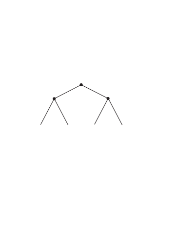
Figure 1: An example of a regular 1-rooted tree; in this case $p=2$. The figure shows the root and the two vertices of the first level, with all the edges incident to them.

Under this identification, the words correspond to vertices, the root is the empty word, and two vertices are joined by an edge if and only if they have the form $a_{1}a_{2}\ldots a_{n}$ and $a_{1}a_{2}\ldots a_{n}a_{n+1}$ for some $n$ and some $a_{i}\in A$. The number $n$ is called the length of a vertex $u=a_{1}a_{2}\ldots a_{n}$ and is denoted by $|u|$. The set of all vertices of length $n$ is called the $n$th level of $T$.

Suppose that $u=\hat{a}_{1}\hat{a}_{2}\ldots\hat{a}_{n}$ is a vertex. The set of all vertices of the form

$$\hat{a}_{1}\hat{a}_{2}\ldots\hat{a}_{n}a_{n+1}a_{n+2}\ldots a_{n+m},$$

where $m\in{\mathbb{N}}$ and $a_{n+i}$ range over the set $A$, forms a subtree of $T$; we will denote this subtree by $T_{u}$. It is easy to see that $T_{u}$ is naturally isomorphic to the same tree $T$ via the map

$$\hat{a}_{1}\hat{a}_{2}\ldots\hat{a}_{n}a_{n+1}a_{n+2}\ldots a_{n+m}\mapsto a_{n+1}a_{n+2}\ldots a_{n+m}.$$

This map allows to identify subtrees $T_{u}$ for all vertices $u$, with one fixed tree $T$.

Their automorphism groups

Let $T$ be a tree as above; an automorphism of $T$ is a bijective map $f$ which fixes the root and preserves the adjacency of vertices. The set of all possible automorphisms of $T$ is obviously a group which we denote by $\mathop{\rm Aut}\nolimits T$; note that it is a profinite group (see also below).

Vertex stabilizers and congruence subgroups

Consider now an arbitrary subgroup $G$ of $\mathop{\rm Aut}\nolimits T$ and a vertex $v$ of $T$. The stabilizer of $v$ in $G$ is the subgroup

$$\mathop{\rm Stab}\nolimits_{G}(v)=\{g\in G\,|\,v^{g}=v\}.$$

Now, if we consider the set of all vertices of level $n$, the subgroup $\cap_{|v|=n}\mathop{\rm Stab}\nolimits_{G}(v)$ is called the ($n$th) level stabilizer and is denoted by $\mathop{\rm Stab}\nolimits_{G}(n)$.

The subgroups $\mathop{\rm Stab}\nolimits_{G}(n)$ are also called principal congruence subgroups in $G$. A subgroup of $G$ which contains a principal congruence subgroup is in turn called a congruence subgroup.

Rigid stabilizers

Let once again $G\leqslant\mathop{\rm Aut}\nolimits T$ and $v\in T$ a vertex. The rigid stabilizer of $v$ in $G$ is the subgroup

$$\mathop{\rm rist}\nolimits_{G}(v)=\{g\in G\,|\,u^{g}=u\mbox{ for all }u\in T\setminus T_{v}\}.$$

We also denote by $\mathop{\rm rist}\nolimits_{G}(n)$ the subgroup $\prod_{|v|=n}\mathop{\rm rist}\nolimits_{G}(v)$; note that this is a normal subgroup of $G$ (unlike the rigid stabilizer of just one vertex).

Recursive presentation of the action of $\mathop{\rm Aut}\nolimits T$

It is easy to see that $\mathop{\rm Aut}\nolimits T$ possesses a sort of “recurrent” structure, that we now describe, as it is extremely useful for working with $\mathop{\rm Aut}\nolimits T$ (and its subgroups). Observe that $\mathop{\rm Aut}\nolimits T$ admits a natural map $\phi:\mathop{\rm Aut}\nolimits T\to\mathop{\rm Aut}\nolimits T\wr\mathop{\rm Sym}\nolimits(A)$, where $\mathop{\rm Sym}\nolimits(A)$ is the group of all permutations of elements of $A$. Thus, every element $x$ of $\mathop{\rm Aut}\nolimits T$ is given by an element

$$f_{x}\in\underbrace{\mathop{\rm Aut}\nolimits T\times\ldots\times\mathop{\rm Aut}\nolimits T}_{|A|}$$

and a permutation $\pi_{x}\in\mathop{\rm Sym}\nolimits(A)$. The latter permutation is called the accompanying permutation, or the activity, of $x$ at the root. We write that

$$\phi(x)=f_{x}\cdot\pi_{x}.$$

In particular, the restriction of $\phi$ onto $\mathop{\rm Stab}\nolimits_{\mathop{\rm Aut}\nolimits T}(1)$ is an embedding (actually, an isomorphism) of $\mathop{\rm Stab}\nolimits_{\mathop{\rm Aut}\nolimits T}(1)$ into (with) the direct product of $|A|$ copies of $\mathop{\rm Aut}\nolimits T$; we will denote this restriction by $\Phi_{1}$. Furthermore, it is easy to see that

$$\Phi_{1}(\mathop{\rm Stab}\nolimits_{\mathop{\rm Aut}\nolimits T}(2))=\underbrace{\mathop{\rm Stab}\nolimits_{\mathop{\rm Aut}\nolimits T}(1)\times\ldots\times\mathop{\rm Stab}\nolimits_{\mathop{\rm Aut}\nolimits T}(1)}_{|A|};$$

therefore we can obtain the isomorphism

$$\Phi_{2}=(\underbrace{\Phi_{1}\times\ldots\times\Phi_{1}}_{|A|})\circ\Phi_{1}:\mathop{\rm Stab}\nolimits_{\mathop{\rm Aut}\nolimits T}(2)\to\underbrace{\mathop{\rm Aut}\nolimits T\times\ldots\mathop{\rm Aut}\nolimits T}_{|A|^{2}}.$$

Proceeding in this manner, we define for each positive integer $n$ the isomorphism

$$\Phi_{n}=(\underbrace{\Phi_{n-1}\times\ldots\times\Phi_{n-1}}_{|A|})\circ\Phi_{1}:\mathop{\rm Stab}\nolimits_{\mathop{\rm Aut}\nolimits T}(n)\to\underbrace{\mathop{\rm Aut}\nolimits T\times\ldots\mathop{\rm Aut}\nolimits T}_{|A|^{n}}.$$

Profinite topology and congruence topology

Let $G\leqslant\mathop{\rm Aut}\nolimits T$; the profinite topology on $G$ is the topology generated by all its finite-index subgroups taken as the system of neighbourhoods of unity. To define the congruence topology, we take the set of all principal congruence subgroups (i.e., the level stabilizers) as the system of neighbourhoods of unity. These two topologies frequently coincide (as it happens for the first of the examples described below) but sometimes they do not (as is the case for the second of the examples that follow).

Examples

Simple examples of the groups described above can be found in [4] or [8] (a different sort). We do not describe them, since we will not need them.

3 A regular tree as a diffeological space

In this section we endow each regular tree $T$ with a diffeology. The condition imperative in making the choice of such is that the corresponding D-topology coincide with the usual one.

3.1 General considerations

A regular rooted tree, such as the ones we are considering, is not naturally a smooth object, and a choice of diffeology with which to endow it, represents its own issue. Although there exist other options, the one we prefer is a certain analogue of the so-called wire diffeology. The latter was introduced by J.M. Souriau as a diffeology on ${\mathbb{R}}^{n}$ alternative to the standard one; it is the diffeology generated by the set $C^{\infty}({\mathbb{R}},{\mathbb{R}}^{n})$, the set of the usual smooth maps ${\mathbb{R}}\to{\mathbb{R}}^{n}$ (thus, its plots are characterized as those maps that locally factor through the smooth maps ${\mathbb{R}}\to{\mathbb{R}}^{n}$). For $n\geqslant 2$ this diffeology is different from the standard one (see [6], Sect. 1.10), although the underlying D-topology is the same (see [3]).

Of course, when we want to carry this notion over to one of our regular trees, the first question to consider is, which maps take the place of smooth ones? We speak about this in detail later on, but in brief, the main points are: the set of all maps ${\mathbb{R}}\to T$ would produce a very, and perhaps unreasonably, large diffeology, the set of all continuous maps still gives a very large one (see below for the curious observation of how the Peano curve enters the picture in this respect), and so it seems reasonable to settle for the set of all embeddings ${\mathbb{R}}\hookrightarrow T$ as the generating set for the wire diffeology on $T$.

3.2 The wire diffeology on $T$

As has already been mentioned, such diffeology is the one generated by some subset of the set of all maps $\{{\mathbb{R}}\to T\}$; the question is, which subset? The following easy considerations suggest to discard the “extreme” possibilities, more specifically: the coarsest of such diffeologies is the one consisting of all maps ${\mathbb{R}}\to T$, whereas the finest one is the discrete diffeology, i.e. the one generated by all constant maps ${\mathbb{R}}\to T$. Neither of the two is very interesting (as is generally the case), and neither respects the structure of $T$ as a topological space, something that we do want to take into account.

This latter consideration suggests to consider continuous maps only, and our options become, to take all continuous maps or only some of them (such as, for instance, the injective ones, which is what we will end up doing). We now illustrate that the diffeology generated by the set of all continuous maps ${\mathbb{R}}\to T$ (which for the moment we will call the coarse wire diffeology) is still very large and, in some very informal sense, loses the $1$-dimensional nature of $T$.

The coarse wire diffeology and the Peano curve

The above statement that the just-mentioned coarse wire diffeology does not truly respect the $1$-dimensional nature of our trees, can actually be observed immediately from the famous example of the Peano curve, a continuous curve that fills the entire unit square. Furthermore, after the appearance in 1890 of the ground-breaking Peano’s example, it became known that any ${\mathbb{R}}^{n}$ (with $n$ an arbitrary positive integer number) is the range of some continuous curve; to be precise, for any $n=2,3,\ldots$ there exists a continuous surjective map $s_{n}:{\mathbb{R}}\to{\mathbb{R}}^{n}$ (hence onto any domain of ${\mathbb{R}}^{n}$). Although none of these maps is invertible, they do allow for a sort of immersion of any other diffeology into the coarsest wire diffeology, by assigning to a given plot $p:{\mathbb{R}}^{n}\supseteq U\to T$ the composition $p\circ t_{U}\circ s_{n}$ (where $t_{U}$ is some diffeomorphism ${\mathbb{R}}^{n}\to U$, fixed for each $U$). Although this assignment would not be one-to-one, it does give an (intuitive, if nothing else) idea of how large the coarse wire diffeology is.

The embedded wire diffeology on $T$

This is the diffeology that we settle one; it is the diffeology generated by all injective and continuous in both directions maps ${\mathbb{R}}\to T$. It depends on $T$ only, so we denote it by ${\mathcal{D}}_{T}$. We furthermore denote the generating set of ${\mathcal{D}}_{T}$, the set $\{f:{\mathbb{R}}\to T\,|\,f\mbox{ is injective and both ways continuous}\}$, by $\tilde{{\mathcal{P}}}_{T}$.

The first thing that we would like to do is to restrict this generating set as much as possible; indeed, if two maps, $f_{1},f_{2}:{\mathbb{R}}\to T$, are such that $f_{2}=f_{1}\circ g$ for some diffeomorphism $g:{\mathbb{R}}\to{\mathbb{R}}$ then (as it follows from the definition of a generated diffeology) only one of them needs to belong to the generating set. Therefore we denote by ${\mathcal{P}}_{T}$ the quotient of $\tilde{{\mathcal{P}}}_{T}$ by the (right) action of the group of diffeomorphisms of ${\mathbb{R}}$; when it does not create confusion, by one or more elements of ${\mathcal{P}}_{T}$ we will mean a corresponding collections of maps that are specific representatives of some equivalence classes. The above observations then prove the following:

Claim 3.1.

The diffeology ${\mathcal{D}}_{T}$ is generated by ${\mathcal{P}}_{T}$.

The topology

We now proceed to showing that the diffeology chosen does satisfy the condition that we wanted to, namely, that the following is true.

Theorem 3.2.

The D-topology corresponding to ${\mathcal{D}}_{T}$ is the usual topology of $T$.

Proof.

Recall that by the definition of D-topology a set $X^{\prime}\subset T$ is D-open if and only if for any plot $p:U\to T$ the pre-image $p^{-1}(X)$ is open in $U$; now, by construction and by the definition of the generated diffeology this is equivalent to $\gamma^{-1}(X)$ being open in ${\mathbb{R}}$ for any $\gamma\in{\mathcal{P}}_{T}$.

We need to show that $X^{\prime}$ is D-open if and only if it is open in $T$ in the usual sense. Suppose first that $X^{\prime}$ is open. Then its pre-image with respect to any $\gamma$ is open in ${\mathbb{R}}$ because $\gamma$ is continuous; therefore it is D-open by the very definition of D-openness.

Now suppose that $X^{\prime}$ is a D-open set; we need to show that it is also open in the usual sense. To do so, it is sufficient to show that for any point of $X^{\prime}$ the latter contains its open neighbourhood. Choose such an arbitrary point $x\in X^{\prime}$; we consider two cases.

Suppose first that $x$ belongs to the interior of some edge $e$. Set $X=X^{\prime}\cap\mbox{Int}(e)$, and let $\gamma\in{\mathcal{P}}_{T}$; we can assume that its image contains $e$. Note that since $\gamma$ is injective, we have $\gamma^{-1}(X)=\gamma^{-1}(X^{\prime})\cap\gamma^{-1}(\mbox{Int}(e))$; both of these two sets are open in ${\mathbb{R}}$, the first because $X^{\prime}$ is D-open and the second because it is the pre-image of an open set under the continuous map $\gamma$. This implies that $\gamma^{-1}(X)$ is open in ${\mathbb{R}}$, therefore $X$ is open in the image of $\gamma$, the latter being a homeomorphism with its image, and it is open in $\mbox{Int}(e)$, hence it is open in $T$ as well. Thus, $X$ is an open neighbourhood of $x$ contained in $X^{\prime}$.

Suppose now that $x$ is a vertex (we can assume that it is not the root; the proof changes only formally for the latter). Let $e_{1},\ldots,e_{p+1}$ be the edges incident to $x$. For each $1\leqslant i<j\leqslant p+1$ let $X_{i,j}=\mbox{Int}(e_{i})\cup\mbox{Int}(e_{j})\cup\{x\}$; set

$$X=\cup_{i,j}(X^{\prime}\cap X_{i,j}).$$

We need to show that $X$ is open in $T$. For each $i,j$ choose a map $\gamma_{i,j}$ such that its image contains $e_{i}\cup e_{j}$. Then $\gamma_{i,j}^{-1}(X^{\prime}\cap X_{i,j})=\gamma_{i,j}^{-1}(X^{\prime})\cap\gamma_{i,j}^{-1}(X_{i,j})$; both of these sets are open in ${\mathbb{R}}$, by the D-openness of $X^{\prime}$ and by continuity of $\gamma$. Hence $\gamma_{i,j}^{-1}(X^{\prime}\cap X_{i,j})$ is open in ${\mathbb{R}}$ and, $\gamma_{i,j}$ being a homeomorphism with its image, the set $X^{\prime}\cap X_{i,j}$ is open in $e_{i}\cup e_{j}$. It follows that $X$ is open in $e_{1}\cup\ldots\cup e_{p+1}$ and therefore it is open in $T$; thus, it is an open nieghbourhood of $x$ contained in $X^{\prime}$, and this concludes the proof. ∎

4 $\mathop{\rm Aut}\nolimits T$ as a diffeological group

In this section we consider $T$ endowed with the embedded wire diffeology described in the previous section. We must first ensure that the elements of $\mathop{\rm Aut}\nolimits T$ are smooth maps with respect to this diffeology; this then gives rise to the functional diffeology on $\mathop{\rm Aut}\nolimits T$ and to the a priori finer diffeology that makes $\mathop{\rm Aut}\nolimits T$ into a diffeological group and is the finest one with such property.

4.1 The functional diffeology on $\mathop{\rm Aut}\nolimits T$

In this section we first make some observations regarding the plots of the functional diffeology on $\mathop{\rm Aut}\nolimits T$; as a preliminary, we need to show that such diffeology is indeed well-defined, i.e., that the elements of $\mathop{\rm Aut}\nolimits T$ are indeed diffeomorphisms. We then proceed to consider the D-topology underlying the functional diffeology of $\mathop{\rm Aut}\nolimits T$.

Automorphisms as diffeomorphisms

The following statement follows easily from the choice of diffeology on $T$.

Proposition 4.1.

Let $g\in\mathop{\rm Aut}\nolimits T$. Then $g:T\to T$ is a smooth map with respect to the diffeology ${\mathcal{D}}_{T}$.

Proof.

By definition of a generated diffeology and that of a smooth map it is sufficient to show that for any given injective and both ways continuous map $\gamma:{\mathbb{R}}\to T$ the composition $g\circ\gamma$ is again injective and both ways continuous. This follows from the fact that $g$ is an automorphism of $T$, i.e., it is a homeomorphism of $T$ considered with its usual topology; as we have already established that the D-topology of $T$ coincides with the usual one, this proves the claim. ∎

A special family of plots of $T$

In the arguments that follow, we will make use of the following family of plots of $T$. Let $\hat{\gamma}$ be an infinite path in $T$; let $v_{0}\in\hat{\gamma}$ be the vertex of the smallest length. For each $\hat{\gamma}$ we fix a homeomorphism $\gamma:{\mathbb{R}}\to\hat{\gamma}\subset T$ such that

$$\gamma(0)=v_{0},\mbox{and for any }n\in{\mathbb{Z}}\,\,\,\,\gamma(n)\mbox{ is a vertex of length }|v_{0}|+n.$$

Obviously, every $\gamma$ is a plot for the diffeology ${\mathcal{D}}_{T}$. We denote the set of maps $\gamma$, associated to all possible $\hat{\gamma}\subset T$, by

$$\Gamma(T)=\{\gamma\,|\;\hat{\gamma}\mbox{ an infinite path in }T\}.$$

We denote by $\Gamma_{0}(T)$ the subset of $\Gamma(T)$ consisting of all those maps whose image contains the root.

For technical reasons we wish to stress that all maps $\gamma\in\Gamma(T)$ possess, by construction, the following properties:

• for any given $x\in{\mathbb{R}}$, its image $\gamma(x)$ is a vertex if and only if $x\in{\mathbb{Z}}$;

• in particular, the restriction of $\gamma$ on any interval of form $(n,n+1)$ is a homeomorphism with the interior of some edge of $T$.

Smooth curves in $\mathop{\rm Aut}\nolimits T$

Since the D-topology is defined by smooth curves (as mentioned in the first section, see [3]), we first establish the following characterization of those plots of the functional diffeology on $\mathop{\rm Aut}\nolimits T$ that are curves.

Proposition 4.2.

Let $p:{\mathbb{R}}\to\mathop{\rm Aut}\nolimits T$ be a plot for the functional diffeology on $\mathop{\rm Aut}\nolimits T$. Then for all $m,n\in{\mathbb{N}}$ the automorphisms $p(n)$, $p(n+1)$ belong to the same coset of $\mathop{\rm Stab}\nolimits(n)$, and the automorphisms $p(-m)$, $p(-m-1)$ belong to the same coset of $\mathop{\rm Stab}\nolimits(m)$.

Proof.

Recall that by Proposition 1.4 $p$ is a plot if and only if the map $\varphi_{p}:{\mathbb{R}}\times T\to T$ given by $\varphi_{p}(x,v)=p(x)(v)$ is smooth. The latter condition implies, in particular, that for any smooth map $f:{\mathbb{R}}\to{\mathbb{R}}$ and for any injective two ways continuous map $\gamma:{\mathbb{R}}\to T$ the composition $\varphi_{p}\circ(f,\gamma):{\mathbb{R}}\to T$ is a plot of $T$, i.e., that (at least locally) it is the composition $\tilde{\gamma}\circ\tilde{f}$, of some smooth map $\tilde{f}:{\mathbb{R}}\to{\mathbb{R}}$ and some injective two ways continuous $\tilde{\gamma}:{\mathbb{R}}\to T$. In particular, the map $\varphi_{p}\circ(f,\gamma)$ is a continuous map in the usual sense.

Let us now fix a positive integer $n$, a vertex $v$ of length $n$, and a vertex $v^{\prime}$ of length $n+1$ adjacent to $v$. Let $\gamma\in\Gamma_{0}(T)$ be such that $\gamma(n)=v$ and $\gamma(n+1)=v^{\prime}$. By definition of $\varphi_{p}$ we have that

$$(\varphi_{p}\circ(\mbox{Id},\gamma))(n)=\varphi_{p}(n,\gamma(n))=p(n)(v),\mbox{ and}$$

$$(\varphi_{p}\circ(\mbox{Id},\gamma))(n+1)=\varphi_{p}(n+1,\gamma(n+1))=p(n+1)(v^{\prime}).$$

We claim that $p(n)(v)$ and $p(n+1)(v^{\prime})$ are adjacent vertices. That they are vertices, of which the first is has length $n$ and the second one has length $n+1$, is obvious, since $p$ takes values in $\mathop{\rm Aut}\nolimits T$, all of whose elements send vertices to vertices preserving their length. It suffices to show that they are adjacent, i.e., joined by an edge. As we have already observed, the map $\varphi_{p}\circ(\mbox{Id},\gamma)$ is continuous in the usual sense, so it suffices to show that the image of the interval $(n,n+1)$ under it does not contain vertices. Indeed, by its definition $\varphi_{p}\circ(\mbox{Id},\gamma)$ writes as $(\varphi_{p}\circ(\mbox{Id},\gamma))(x)=p(x)(\gamma(x))$; we first observe that this image is a vertex if and only if $\gamma(x)$ is a vertex (this is because $p(x)\in\mathop{\rm Aut}\nolimits T$), then, second, $\gamma(x)$ is a vertex if and only if $x\in{\mathbb{Z}}$ (this is by choice of $\gamma$). In particular, if $n<x<n+1$ then $(\varphi_{p}\circ(\mbox{Id},\gamma))(x)=p(x)(\gamma(x))$ belongs to the interior of some edge, and precisely, the edge that joins $p(n)(v)$ and $p(n+1)(v^{\prime})$.

It remains to observe that $p(n+1)(v^{\prime})$ is adjacent to a unique vertex of length $n$; since $v$ and $v^{\prime}$ are adjacent, $v$ has length $n$, and $p(n+1)$ is an automorphism, this vertex is $p(n+1)(v)$. On the other hand, $p(n)(v)$ has length $n$, and we have just shown that it is adjacent to $p(n+1)(v^{\prime})$; we conclude that

$$p(n)(v)=p(n+1)(v).$$

Finally, since $v$ is arbitrary, we can conclude that $p(n)\mathop{\rm Stab}\nolimits(n)=p(n+1)\mathop{\rm Stab}\nolimits(n)$, as claimed; and since $n$ is arbitrary, this proves the entire statement. ∎

We now can draw the following conclusion.

Corollary 4.3.

Each of the two sequences $\{p(n)\}$, $\{p(-m)\}$ is a converging sequence for the congruence topology on $\mathop{\rm Aut}\nolimits T$.

Note that we phrase this statement in terms of the congruence topology on $\mathop{\rm Aut}\nolimits T$, and not in those of the profinite topology, which for $\mathop{\rm Aut}\nolimits T$ does coincide with the congruence one. This is to highlight the relation of this statement for examples such as the group $\Gamma$, for which the two topologies are different; although we will see shortly a fact that renders the difference insignificant.

Proof.

It suffices to show that $p(n)\mathop{\rm Stab}\nolimits(n)=p(n+k)\mathop{\rm Stab}\nolimits(n)$ for all $n,k\in{\mathbb{N}}$; as in the previous proof, this is equivalent to having $p(n)(v)=p(n+k)(v)$ for any vertex $v$ of length $n$. Choose such a vertex, and fix a map $\gamma\in\Gamma_{0}(T)$ such that $\gamma(n)=v$. As we have established in the proof of the previous proposition, $p(n+1)(\gamma(n+1))$ belongs to the subtree $T_{p(n)(v)}$. By the same reasoning, applied to $n+1$, the vertex $p(n+2)(\gamma(n+2))$ belongs to the subtree $T_{p(n+1)(\gamma(n+1))}\subset T_{p(n)(v)}$. Now, since $\gamma(n+2)\in T_{v}$ by choice of $\gamma$, each vertex of length $n+2$ belongs to a unique subtree $T_{u}$ with $|u|=n$, and $p(n+2)$ is an automorphism, we can conclude that $p(n+2)(v)=p(n)(v)$, and the corollary follows by the now obvious induction on $k$. ∎

The above Corollary actually paves the way to the following statement of crucial consequences:

Proposition 4.4.

Let $p:{\mathbb{R}}\to\mathop{\rm Aut}\nolimits T$ be a plot for the functional diffeology. Then $p$ is a constant map.

Proof.

Recall that by Proposition 1.4 $p$ is a plot if and only if the map $\varphi:{\mathbb{R}}\times T\to T$ given by $\varphi(u,t)=p(u)(t)$ is smooth. Now, by definition $\varphi$ is smooth if and only if for any plot $p^{\prime}:U\to{\mathbb{R}}\times T$ the composition $\varphi\circ p^{\prime}$ is again a plot of $T$.

Let us fix and arbitrary vertex $v$ of $T$, and let us take, as the plot $p^{\prime}$, the following map: $(\mbox{Id}_{{\mathbb{R}}},c_{v}):{\mathbb{R}}\to{\mathbb{R}}\times T$, where $c_{v}:{\mathbb{R}}\to T$ is the constant map acting by $c_{v}(x)\equiv v$. Then

$$(\varphi\circ(\mbox{Id}_{{\mathbb{R}}},c_{v}))(x)=p(x)(v).$$

Observe now that $p(x)$ is an automorphism of $T$ for all $x$, and so sends vertices to vertices; therefore the image of the map $\varphi\circ(\mbox{Id}_{{\mathbb{R}}},c_{v})$ is a set of vertices of $T$. In particular, it is a discrete subset of $T$.

On the other hand, $\varphi\circ(\mbox{Id}_{{\mathbb{R}}},c_{v})$ is a plot of $T$; as such, it is either a constant map or it filters through an injective continuous map ${\mathbb{R}}\to T$ via a smooth map ${\mathbb{R}}\to{\mathbb{R}}$. In this latter case it must a continuous map defined on a connected set and so cannot have a discrete set with more than one point as its image. It remains to conclude that $\varphi\circ(\mbox{Id}_{{\mathbb{R}}},c_{v})$ is a constant map, which means that $p(x)(v)$ does not depend on $x$. Since $v$ is arbitrary, this implies that $p$ is a constant map, as is claimed. ∎

The meaning of this Proposition is that the only smooth curves in $\mathop{\rm Aut}\nolimits T$ are the constant ones; this has far-reaching consequences, as we immediately see.

The D-topology of $\mathop{\rm Aut}\nolimits T$

From what is established in the previous paragraph we easily draw the following conclusion.

Theorem 4.5.

The D-topology underlying the functional diffeology on $\mathop{\rm Aut}\nolimits T$ is the discrete topology.

Proof.

This follows from the Proposition above and Theorem 3.7 of [3] (see also Example 3.2(2) therein). ∎

The functional diffeology of $\mathop{\rm Aut}\nolimits T$ is discrete

Moreover, we consider the proof of Proposition 4.4, we see that the plot $p$ under consideration being defined on ${\mathbb{R}}$ rather than an arbitrary domain $U\subseteq{\mathbb{R}}^{k}$ was not significant; it would hold just the same writing $U$ in place of ${\mathbb{R}}$ and $u\in U$ in place of $x$. This implies that all plots of the functional diffeology of $\mathop{\rm Aut}\nolimits T$ are constant maps, and therefore this diffeology is indeed discrete.

4.2 Functional diffeology of $\mathop{\rm Aut}\nolimits T$ and its diffeological group structure

We shall now make some remarks regarding the diffeological group structure on $\mathop{\rm Aut}\nolimits T$, in relation to its functional diffeology. We have already established that the latter is discrete and therefore is the finest possible diffeology on $\mathop{\rm Aut}\nolimits T$ (see [6], Section 1.20). For this reason it coincides with the diffeological group structure, the latter being a priori finer than the functional diffeology.

University of Pisa
Department of Mathematics
Via F. Buonarroti 1C
56127 PISA – Italy
 
ekaterina.pervova@unipi.it

References

- [1] S.V. Alyoshin, Finite automata and the Burnside problem for periodic groups, Mat. Zametki (3) 11 (1986), pp. 319-328.
- [2] J.D. Christensen – E. Wu, The homotopy theory of diffeological spaces, New York J. Math. 20 (2014), pp. 1269-1303.
- [3] J.D. Christensen – G. Sinnamon – E. Wu, The D-topology for diffeological spaces, arXiv.math 1302.2935v3.
- [4] R.I. Grigorchuk, Degrees of growth of finitely generated groups and the invariant mean, Izv. Ross. Akad. Nauk Ser. Mat. (1984), (5) 48, pp. 939-996.
- [5] P. Iglesias-Zemmour – Y. Karshon – M. Zadka, Orbifolds as diffeologies, Trans. Amer. Math. Soc. (2010), (6) 362, pp. 2811-2831.
- [6] P. Iglesias-Zemmour, Diffeology, Mathematical Surveys and Monographs, 185, AMS, Providence, 2013.
- [7] E. Pervova, Subgroup structure of AT-groups, Ph.D. thesis, Ekaterinburg (2003).
- [8] E. Pervova, Profinite completions of some groups acting on trees, J. Algebra 310 (2007), pp. 858-879.
- [9] J.M. Souriau, Groups différentiels, In Differential geometrical methods in mathematical physics (Proc. Conf., Aix-en-Provence/Salamanca, 1979), Lecture Notes in Mathematics, 836, Springer, (1980), pp. 91-128.
- [10] J.M. Souriau, Groups différentiels de physique mathématique, South Rhone seminar on geometry, II (Lyon, 1984), Astérisque 1985, Numéro Hors Série, pp. 341-399.
- [11] A. Stacey, Comparative smootheology, Theory Appl. Categ., 25(4) (2011), pp. 64-117.