YITP-15-41

We study a new class of supersymmetric solutions in five-dimensional supergravity representing multi-center configurations of codimension-2 branes along arbitrary curves. Codimension-2 branes are produced in generic situations out of ordinary branes of higher codimension by the supertube effect and, when they are exotic branes, spacetime generally becomes non-geometric. The solutions are characterized by a set of harmonic functions on $\mathbb{R}^{3}$ with non-trivial monodromies around codimension-2 branch-point singularities. The solutions can be regarded as generalizations of the Bates-Denef/Bena-Warner multi-center solutions with codimension-3 centers to include codimension-2 ones. We present some explicit examples of solutions with codimension-2 centers, and discuss their relevance for the black microstate (non-)geometry program.

1 Introduction

String theory contains various branes that come in diverse dimensions, such as D-branes, and they have played a crucial role in understanding the non-perturbative aspects of string theory. Among these branes, ones with small $(\leq 2)$ codimension have been relatively less studied, probably due to their non-standard features. For instance, the codimension-2 D7-brane destroys the spacetime asymptotics by introducing conical deficit, and the codimension-1 D8-brane terminates spacetime a finite distance from it as the dilaton diverges. However, it is such peculiarities that make small-codimension branes special and all the more interesting. For example, the fact that 7-branes change spacetime asymptotics is precisely what makes the F-theory geometries work [1, 2]. More recently, it was pointed out [3, 4] that small-codimension branes can be spontaneously created out of ordinary (codimension $>2$) branes by the supertube transition [5] and generically lead to non-geometric spacetime. In particular, black holes in string theory are typically constructed by intersecting multiple stacks of branes, which can spontaneously polarize by the supertube transition into small-codimension branes. So, studying small-codimension branes and the accompanying non-geometric structure of spacetime is relevant for understanding microscopic physics of black holes in string theory.

Five-dimensional supergravity has been extensively used as a convenient paradigm in which to study black holes in string theory. In particular, all supersymmetric solutions of $d=5$, ${\cal N}=1$ ungauged supergravity with vector multiplets have been completely classified in [6, 7]. This supergravity theory describes the low-energy physics of M-theory compactified on a Calabi-Yau 3-fold $X$ or, in the presence of an additional $S^{1}$ [9, 6], of type IIA string theory compactified on $X$. In the latter picture, these supersymmetric solutions represent a system of D6, D4, D2, and D0-branes wrapped on various cycles inside $X$ [14]. Let us call this solution of $d=5$ supergravity the “4D/5D solution.” The 4D/5D solution is completely specified by a set of harmonic functions, which we collectively denote by $H$, on a spatial ${\mathbb{R}}^{3}$ base. Its general form is

$$H({\mathbf{x}})=h+\sum_{p=1}^{N}{\Gamma_{p}\over|{\mathbf{x}}-{\mathbf{a}}_{p}|}\,,$$ (1.1)

and the associated 4D/5D solution represents a bound state of $N$ black hole centers, which are sitting at ${\mathbf{x}}={\mathbf{a}}_{p}$ ($p=1,\dots,N$) and are made of D6, D4, D2, and D0-branes represented by the coefficients $\Gamma_{p}$. The black hole centers are of codimension 3, being a point in the ${\mathbb{R}}^{3}$. The 4D/5D solution has been applied to various studies of black holes and rings in four and five dimensions, such as the black hole attractor mechanism [15, 16, 17, 18, 19, 20, 21], split attractor flows and wall crossing [22, 23, 24, 25, 14], and microstate geometries [26, 27].

The supertube transition [5] is a spontaneous polarization phenomenon in which a particular combination of branes puffs up into a new dipole charge. For example, if we put two orthogonal D2-branes together, they will polarize into an NS5-brane along an arbitrary closed curve parametrized by $\lambda$. We represent this process as follows:

$$\rm D2(45)+D2(67)\to ns5(\lambda 4567)\,,$$ (1.2)

where D2(45) denotes the D2-brane wrapped around 45 directions and “ns5” in lowercase means that it is a dipole charge. We assume that 4567 directions are compact. As we have mentioned, such D2-branes appear in the 4D/5D solution described by (1.1), and the supertube transition (1.2) implies that the solution must actually be extended to include codimension-2 sources along arbitrary curves in the ${\mathbb{R}}^{3}$, in order to describe the full configuration space of the brane system.

As we will see in explicit examples later, this does not just mean to smear the codimension-3 singularities in the harmonic function (1.1) along a curve to get a codimension-2 singularity, but the harmonic function can also have branch-point singularities and be multi-valued in ${\mathbb{R}}^{3}$. It is a generic feature of codimension-2 branes that, as one goes around their worldvolume, the spacetime fields undergo a U-duality transformation [3, 4] and become multi-valued; the harmonic function being multi-valued is the manifestation of this.

For the transition (1.2), it is only the $B$-field that are multi-valued around the supertube (ns5). However, there are also supertube transitions that produce non-geometric exotic branes, around which the metric is multi-valued. One example is

$$\rm D2(89)+D6(456789)\to 5^{2}_{2}(\lambda 4567;89)\,,$$ (1.3)

where $5^{2}_{2}$ is a non-geometric exotic brane which are obtained by two transverse T-dualities of the NS5-brane and have been much studied in the recent literature [3, 4, 29, 30, 31, 32, 33, 34, 35, 36, 37, 38, 39, 40, 41, 42, 43, 44]. This process exemplifies the fact that standard branes can generally turn into exotic branes with non-geometric spacetime.

The purpose of the present paper is to demonstrate how configurations with codimension-2 sources, geometric and non-geometric, can be represented in the 4D/5D solution. To our knowledge, the 4D/5D solution with codimension-2 sources has not been investigated before, and represents a large unexplored area of research. For the codimension-3 case, Eq. (1.1) gives the general multi-center solution. More generally, however, the codimension-3 centers must polarize into supertubes, thus giving a multi-center solution of codimension-3 and codimension-2 centers. It is technically challenging to explicitly construct general multi-center solutions involving codimension-2 centers. So, in this paper, we present some simple but explicit solutions which must be useful for finding the general solutions. An obvious application of codimension-2 solutions is to generalize the studies previously done for codimension-3 sources to include codimension-2 sources mentioned above. In [3, 4], it was argued that codimension-2 play an essential role in the microscopic physics of black holes and we hope that this paper will set a stage for research in that direction.

The plan of the rest of the paper is as follows. In section 2, we start by reviewing 5D supergravity and the “4D/5D solution” which is supersymmetric and characterized by a set of harmonic functions on ${\mathbb{R}}^{3}$. We explain that, although normally the harmonic functions are assumed to have codimension-3 source, they can more generally have codimension-2 source as well. In section 3, we present some example solutions with codimension-2 source in the harmonic functions. The examples include supertubes with standard and exotic dipole charges and, in the latter case, the spacetime is non-geometric. In section 4, we give an example in which codimension-3 source and codimension-2 one coexist. We conclude in section 5 with remarks on the fuzzball conjecture and the microstate geometry program. The appendices explain our convention and some detail of the computations in the main text.

2 Setup

2.1 The 4D/5D solution

We start from $d=5$, $\mathcal{N}=1$ ungauged supergravity coupled to two vector multiplets. Including the graviphoton the theory contains three vector fields $A^{I}$ ($I=1,2,3$) and two independent scalar fields which can be parametrized by $X^{I}$ satisfying the constraint $\frac{1}{6}C_{IJK}X^{I}X^{J}X^{K}=1$. Here, $C_{IJK}$ are constants that are symmetric under permutations of $IJK$, and are given by $C_{IJK}=|\epsilon_{IJK}|$ in our case. The bosonic action of this theory is

$$S=\frac{1}{16\pi G_{5}}\int\left(-R*1+Q_{IJ}*F^{I}\wedge F^{J}+Q_{IJ}*dX^{I}\wedge dX^{J}-\frac{1}{6}C_{IJK}F^{I}\wedge F^{J}\wedge A^{K}\right)\,,$$ (2.1)

where $*$ means the five-dimensional Hodge dual and $F^{I}=dA^{I}$. The metric for the kinetic term is

$$Q_{IJ}=\frac{1}{2}\operatorname{diag}\left((X^{1})^{-2},(X^{2})^{-2},(X^{3})^{-2}\right)\,.$$ (2.2)

The supersymmetric solutions of this theory have been completely classified [6, 8, 7, 9] by solving Killing spinor equations. There are two classes of supersymmetric solutions, depending on whether the Killing vector constructed from the Killing spinor bilinear is null or timelike. Here we will only consider the latter case. For the timelike class solution, the metric and gauge fields are given by

$$ds^{2}_{5} =-Z^{-2/3}\left(dt+k\right)^{2}+Z^{1/3}ds_{\mathrm{HK}}^{2}\,,\qquad Z=Z_{1}Z_{2}Z_{3}\,,$$ (2.3)

$$A^{I} =B^{I}-Z_{I}^{-1}(dt+k)\,,$$

where the functions $Z_{I}$ and the 1-forms $k,B^{I}$ depend only on the coordinates of the 4D base with the hyper-Kähler metric $ds_{\mathrm{HK}}^{2}$. The scalars $X^{I}$ are related to the electric potential $Z_{I}$ by

$$X^{I}=Z^{1/3}Z_{I}^{-1}\,.$$ (2.4)

It will be convenient to define the magnetic field strength by

$$\Theta^{I}=dB^{I}\,.$$ (2.5)

The demand of supersymmetry leads to the following BPS equations to be satisfied by the quantities $\Theta^{I}$, $Z_{I}$, and $k$:

$$\Theta^{I} =*_{4}\Theta^{I}\,,$$ (2.6a)

$$d*_{4}dZ_{I} =\frac{1}{2}C_{IJK}\Theta^{J}\wedge\Theta^{K}\,,$$ (2.6b)

$$(1+*_{4})dk =Z_{I}\Theta^{I}\,,$$ (2.6c)

where $*_{4}$ is the Hodge dual with respect to the 4D metric $ds^{2}_{\text{HK}}$. If we solve these equations in the order presented, the problem is linear; namely, at each step, we have a Poisson equation with the source given in terms of the quantities found in the previous step.

If we assume the presence of an additional translational Killing vector that preserves the hyper-Kähler structure (namely, if the Killing vector is tri-holomorphic), the 4D base should be a Gibbons-Hawking space [45] and its metric must take the following form [46]:

$$ds_{\mathrm{HK}}^{2}=V^{-1}(d\psi+A)^{2}+V\delta_{ij}dx^{i}dx^{j}\,,\qquad i,j=1,2,3\,.$$ (2.7)

Here, the 1-form $A$ and the scalar $V$ depend only on the coordinates $x^{i}$ of the $\mathbb{R}^{3}$ base and satisfy

$$dA=*_{3}dV\,.$$ (2.8)

The isometry direction $\psi$ has periodicity $4\pi$. The orientation of the 4-dimensional base is given by

$$\epsilon_{\psi 123}=+\sqrt{g_{\mathrm{HK}}}=V\,.$$ (2.9)

From (2.8), it is easy to see that $V$ is a harmonic function on ${\mathbb{R}}^{3}$,

$${\bigtriangleup}V=0\,,\qquad{\bigtriangleup}=\partial_{i}\partial_{i}\,.$$ (2.10)

Solving the BPS equations

If we decompose $\Theta^{I}$ and $k$ according to the fiber-base decomposition of the Gibbons-Hawking metric (2.7), we can solve all the BPS equations (2.6) in terms of harmonic functions on ${\mathbb{R}}^{3}$. For later convenience, let us recall how this goes in some detail [9].

First, by self-duality (2.6a), the 2-form $\Theta^{I}$ can be written as

$$\Theta^{I}=(d\psi+A)\wedge\theta^{I}+V*_{3}\theta^{I}\,,$$ (2.11)

where $\theta^{I}$ is a 1-form on ${\mathbb{R}}^{3}$ and $*_{3}$ is the Hodge dual on ${\mathbb{R}}^{3}$. The closure $d\Theta^{I}=0$ (the part multiplying $d\psi+A$) implies $d\theta^{I}=0$, which means that $\theta^{I}=d\Lambda^{I}$ with a scalar $\Lambda^{I}$. If we plug this equation back into $d\Theta^{I}=0$, we find

$${\bigtriangleup}(V\Lambda^{I})=0\,.$$ (2.12)

Therefore, $\Lambda^{I}=-V^{-1}K^{I}$ with $K^{I}$ harmonic, and

$$\Theta^{I}=-(d\psi+A)\wedge d(V^{-1}K^{I})-V*_{3}d(V^{-1}K^{I})\,.$$ (2.13)

Next, plugging (2.13) into (2.6b), we find that $Z_{I}$ satisfies the following Laplace equation:

$${\bigtriangleup}Z_{I}=C_{IJK}V\,\partial_{i}(V^{-1}K^{J})\,\partial_{i}(V^{-1}K^{K})={1\over 2}C_{IJK}{\bigtriangleup}(V^{-1}K^{J}K^{K})\,,$$ (2.14)

where in the last equality we used harmonicity of $V,K^{I}$. This means that

$$Z_{I}=L_{I}+{1\over 2}C_{IJK}V^{-1}K^{J}K^{K}\,,$$ (2.15)

where $L_{I}$ is harmonic.

Furthermore, if we decompose the 1-form $k$ as

$$k=\mu(d\psi+A)+\omega\,,$$ (2.16)

where $\omega$ is a 1-form on ${\mathbb{R}}^{3}$, we can show that the condition (2.6c) leads to another Laplace equation:

$${\bigtriangleup}\mu=V^{-1}\partial_{i}[VZ_{I}\partial_{i}(V^{-1}K^{I})]={\bigtriangleup}\Bigl{(}{1\over 2}V^{-1}K^{I}L_{I}+{1\over 6}C_{IJK}V^{-2}K^{I}K^{J}K^{K}\Bigr{)}\,.$$ (2.17)

In the last equality, we used harmonicity of $V,K^{I},L_{I}$. Therefore, $\mu$ is given in terms of another harmonic function $M$ as

$$\mu=M+{1\over 2}V^{-1}K^{I}L_{I}+{1\over 6}C_{IJK}V^{-2}K^{I}K^{J}K^{K}\,.$$ (2.18)

The 1-form $\omega$ is found by solving the equation

$$*_{3}d\omega=VdM-MdV+\frac{1}{2}\left(K^{I}dL_{I}-L_{I}dK^{I}\right)$$ (2.19)

that also follows from (2.6c). By taking $d\,*_{3}$ of this equation, we can derive the so-called integrability equation:

$$0=V{\bigtriangleup}M-M{\bigtriangleup}V+\frac{1}{2}\left(K^{I}{\bigtriangleup}L_{I}-L_{I}{\bigtriangleup}K^{I}\right)\,.$$ (2.20)

This must be satisfied for the 1-form $\omega$ to exist. Although we allow delta-function sources for the Laplace equations (2.10), (2.12), (2.14) and (2.17), this equation (2.20) must be imposed without allowing any delta function in order for $\omega$ to exist.

Finally, we note that the magnetic potential $B^{I}$ can be written as

$$B^{I}=V^{-1}K^{I}(d\psi+A)+\xi^{I}\,,\qquad d\xi^{I}=-*_{3}dK^{I}\,.$$ (2.21)

In summary, under the assumption of the additional $U(1)$ symmetry, we can solve all the equations (2.6) in terms of harmonic functions $V,K^{I},L_{I},M$. We will refer to this solution as the “4D/5D solution.”

The 10 and 11-dimensional uplift

The 5D solution (2.3) can be thought of as coming from 11D M-theory compactified on $T^{6}=T^{2}_{45}\times T^{2}_{67}\times T^{2}_{89}$, with the following metric and the 3-form potential:

$$\begin{split}ds_{11}^{2}&=-Z^{-2/3}(dt+k)^{2}+Z^{1/3}ds_{\mathrm{HK}}^{2}+Z^{1/3}\left(Z_{1}^{-1}dx_{45}^{2}+Z_{2}^{-1}dx_{67}^{2}+Z_{3}^{-1}dx_{89}^{2}\right)\,,\\ {\cal A}_{3}&=A^{I}J_{I}\,,\qquad J_{1}\equiv dx^{4}\wedge dx^{5}\,,\quad J_{2}\equiv dx^{6}\wedge dx^{7}\,,\quad J_{3}\equiv dx^{8}\wedge dx^{9}\,,\end{split}$$ (2.22)

where $dx_{45}^{2}\equiv(dx^{4})^{2}+(dx^{5})^{2}$ and so on. The scalars $X^{I}=Z^{1/3}Z_{I}^{-1}$ correspond to the volume of the 2-tori. M-theory on $T^{6}$ has ${\cal N}=4$ supersymmetry (32 supercharges) in 5D, and the theory (2.1) gives its ${\cal N}=1$ truncation in which only 8 supercharges are kept.

In the presence of the isometry direction $\psi$ in the 4D base as in (2.7), the above 11D configuration (2.22) can be reduced on it to a 10D type IIA configuration using the formula (A.1) as follows:

$$\begin{split}ds_{\mathrm{10,str}}^{2}&=-{1\over\sqrt{V(Z-V\mu^{2})}}(dt+\omega)^{2}+\sqrt{V(Z-V\mu^{2})}\,dx^{i}dx^{i}\\ &\qquad\qquad+\sqrt{Z-V\mu^{2}\over V}\left(Z_{1}^{-1}dx_{45}^{2}+Z_{2}^{-1}dx_{67}^{2}+Z_{3}^{-1}dx_{89}^{2}\right)\,,\\ e^{2\Phi}&={(Z-V\mu^{2})^{3/2}\over V^{3/2}Z}\,,\qquad B_{2}=\left(V^{-1}K^{I}-Z_{I}^{-1}\mu\right)J_{I}\,,\\ C_{1}&=A-{V\mu\over Z-V\mu^{2}}(dt+\omega)\,,\\ C_{3}&=\left[(V^{-1}K^{I}-Z_{I}^{-1}\mu)A+\xi^{I}-Z_{I}^{-1}(dt+\omega)\right]\wedge J_{I}\,.\end{split}$$ (2.23)

We note that the complexified Kähler moduli $\tau^{1}$, $\tau^{2}$, and $\tau^{3}$ for the 2-tori $T^{2}_{45}$, $T^{2}_{67}$, and $T^{2}_{89}$, respectively, are

$$\tau^{1}={R_{4}R_{5}\over l_{s}^{2}}\Bigl{(}B_{45}+i\sqrt{\det G_{ab}}\Bigr{)}={R_{4}R_{5}\over l_{s}^{2}}\left[\left({K^{1}\over V}-{\mu\over Z_{1}}\right)+i\frac{\sqrt{V(Z-V\mu^{2})}}{Z_{1}V}\right]\,,$$ (2.24)

where $a,b=4,5$, and similarly for $\tau^{2},\tau^{3}$. We denoted the radii of $x^{i}$ directions by $R_{i},i=4,\cdots,9$. If we compactify the theory to 4D, these $\tau^{I}$ become scalar moduli parametrizing the moduli space $[SL(2,{\mathbb{R}})/SO(2)]^{3}$.

2.2 Codimension-3 sources

As we have seen above, the 4D/5D solution is specified by the set of harmonic functions $V,K^{I},L_{I},M$. The general harmonic functions with codimension-3 sources are [14, 9]

$$V =h^{0}+\sum_{p=1}^{N}{\Gamma^{0}_{p}\over|{\mathbf{x}}-{\mathbf{a}}_{p}|}\,, \qquad K^{I} =h^{I}+\sum_{p=1}^{N}{\Gamma^{I}_{p}\over|{\mathbf{x}}-{\mathbf{a}}_{p}|}\,,$$ (2.25)

$$L_{I} =h_{I}+\sum_{p=1}^{N}{\Gamma_{I}^{p}\over|{\mathbf{x}}-{\mathbf{a}}_{p}|}\,, M =h_{0}+\sum_{p=1}^{N}{\Gamma_{0}^{p}\over|{\mathbf{x}}-{\mathbf{a}}_{p}|}\,,$$

where ${\mathbf{x}}=(x^{1},x^{2},x^{3})$, and ${\mathbf{a}}_{p}\in{\mathbb{R}}^{3}$ is the position of the sources at which the harmonic functions become singular. The integrability condition (2.20) demands that the position of the centers satisfy

$$\sum_{q(\neq p)}{{\langle{\Gamma_{p},\Gamma_{q}}\rangle}\over a_{pq}}={\langle{h,\Gamma_{p}}\rangle}$$ (2.26)

where ${\langle{u,v}\rangle}\equiv u^{0}v_{0}-u_{0}v^{0}+{1\over 2}(u^{I}v_{I}-u_{I}v^{I})$ and $a_{pq}\equiv|{\mathbf{a}}_{p}-{\mathbf{a}}_{q}|$. See Fig. -59(a) for a schematic explanation of codimension-3 solutions. When we embed the 5D supergravity in string/M-theory, these singularities are interpreted as brane sources. For example, in the type IIA picture (2.23), the singularities in the harmonic functions (2.25) have the following interpretation as brane sources [14]:

$$V\leftrightarrow\text{D6(456789)}\,,\quad\begin{array}[]{l}K^{1}\leftrightarrow\text{D4(6789)}\\ K^{2}\leftrightarrow\text{D4(4589)}\\ K^{3}\leftrightarrow\text{D4(4567)}\\ \end{array}\,,\quad\begin{array}[]{l}L_{1}\leftrightarrow\text{D2(45)}\\ L_{2}\leftrightarrow\text{D2(67)}\\ L_{3}\leftrightarrow\text{D2(89)}\\ \end{array}\,,\quad M\leftrightarrow\text{D0}\,.$$ (2.27)

Note that, in our description, the branes are always smeared along all transverse directions inside the compact directions ($456789$). For example, the D4(6789)-brane is smeared along the $45$ directions. So, all the branes in (2.27) can be regarded as having codimension 3 (pointlike in ${\mathbb{R}}^{3}$).

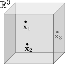
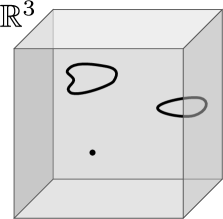
(a)	(b)

Figure -59: The 4D/5D solution is specified by harmonic functions on the base ${\mathbb{R}}^{3}$. (a) The codimension-3 solution is specified by point-like singularities of the harmonic functions. (b) The general solution involves point-like (codimension-3) as well as string-like (codimension-2) singularities in the harmonic functions.

Many known black hole and black ring solutions in 4D and 5D are included in the 4D/5D solutions with the harmonic functions having codimension-3 singularities, (2.25). For example, the 3-charge black hole in 5D with the charges of M2(45), M2(67), M2(89)-branes, which is dual to the Strominger-Vafa black hole [47], can be expressed by the following harmonic functions:

$$V=\frac{1}{r}\,,\qquad K^{I}=0\,,\qquad L_{I}=1+\frac{Q_{I}}{r}\,,\qquad M=0\,.$$ (2.28)

Other examples include the BMPV black hole [48], the supersymmetric black ring [49, 7, 50], the MSW black hole [51], multi-center black hole/ring solutions [14] and microstate geometries [26, 27].

2.3 Codimension-2 sources

In the previous subsection, we considered the 4D/5D solution which has only codimension-3 sources of D-branes. However, recall that, in string theory, certain combinations of branes can undergo a supertube transition [5], under which branes spontaneously polarize into new dipole charge, gaining size in transverse directions. For example, as we have discussed in the Introduction, two transverse D2-branes can polarize into an NS5-brane along an arbitrary closed curve $\lambda$, as in (1.2). Because the NS5-brane is along a closed curve, it has no net NS5 charge but only NS5 dipole charge. The original D2 charges are dissolved in the NS5 worldvolume as fluxes. When the curve $\lambda$ is inside the $\mathbb{R}^{3}_{123}$, which is generically the case and is assumed henceforth, the NS5-brane appears as a codimension-2 object in the non-compact 123 directions. Therefore, if we are to consider generic solutions describing D-brane systems, we must include codimension-2 brane sources in the 4D/5D solution. Even in such situations, the procedure (2.13)–(2.18) to solve the BPS equations goes through and the solution is given by the harmonic functions $V,K^{I},L_{I},M$. However, they are now allowed to have codimension-2 singularities in ${\mathbb{R}}^{3}$. See Fig. -59(b) for a schematic explanation for solutions with codimension-2 sources.

To get some idea about solutions with codimension-2 sources, here we present the harmonic functions for the $\rm D2+D2\to ns5$ supertube (1.2) when the puffed-up ns5-brane is an infinite straight line along $x^{3}$.

$$V =1\,,\qquad K^{1}=K^{2}=0\,,\quad K^{3}=q\mspace{1.0mu}\theta\,,$$ (2.29)

$$L_{1} =1+Q_{1}\log{\Lambda\over r}\,,\quad L_{2}=1+Q_{2}\log{\Lambda\over r}\,,\quad L_{3}=1\,,\qquad M=-{1\over 2}q\mspace{1.0mu}\theta\,,$$

where $q=l_{s}^{2}/(2\pi R_{8}R_{9})$, $Q_{1}Q_{2}=q^{2}$, and $\Lambda$ is a constant. We took the cylindrical coordinates for the ${\mathbb{R}}^{3}$ base,

$$ds_{3}^{2}=dr^{2}+r^{2}d\theta^{2}+(dx^{3})^{2}\,.$$ (2.30)

We will discuss such solutions more generally in the next sections. A novel feature is that the harmonic function $K^{3}$ has a branch-point singularity along the $x^{3}$ axis at $r=0$. So, $K^{3}$ does not just have a codimension-2 singularity but is multi-valued. This $K^{3}$ cannot be obtained by smearing a $K^{3}$ with codimension-3 singularities as in (2.25). As one can see from (2.23), this $K^{3}$ leads to the $B$-field

$$B_{2}={l_{s}^{2}\theta\over 2\pi R_{8}R_{9}}dx^{8}\wedge dx^{9}\,.$$ (2.31)

Around the $x^{3}$-axis, this has monodromy $\Delta B_{2}=l_{s}^{2}/(R_{8}R_{9})$, which is the correct one for an NS5-brane extending along 34567 directions and smeared along 89 directions. On the other hand, the codimension-2 singularities in $L_{1},L_{2}$ represent the D2-brane sources dissolved in the NS5 and are obtained by smearing codimension-3 singularities in (2.25). The monodromy in $M$ (2.29) does not have direct physical significance here, because what enters in physical quantities is $\mu$, which is trivial in the present case: $\mu=M+{1\over 2}K^{3}L_{3}=0$.

In the lower dimensional (4D) picture, the $B$-field appears as the scalar moduli $\tau^{I}$ defined in (2.24). For the present case (2.31), we have

$$\tau^{3}={\theta\over 2\pi}\,.$$ (2.32)

As we go around $r=0$, the modulus $\tau^{3}$ has the monodromy

$$\tau^{3}\to\tau^{3}+1\,,$$ (2.33)

which can be understood as an $SL(2,{\mathbb{Z}})$ duality transformation. It was emphasized in [3, 4] that the charge of the codimension-2 brane is measured by the duality monodromy around it. It is possible to consider codimension-2 objects around which there is more general $SL(2,{\mathbb{Z}})$ monodromy of $\tau^{I}$. For example, if we have an object around which there is the following monodromy:

$$\tau^{3}\to{\tau^{3}\over-\tau^{3}+1}\,,\qquad\text{or}\quad\tau^{\prime 3}\to\tau^{\prime 3}+1\,,\quad\tau^{\prime 3}\equiv-{1\over\tau^{3}}\,,$$ (2.34)

it corresponds to an exotic brane called the $5^{2}_{2}(34567,89)$-brane [3, 4]. This brane is non-geometric since the $T^{2}_{89}$ metric is not single-valued but is twisted by a $T$-duality transformation around it. The $5^{2}_{2}$-brane is produced in the supertube transition (1.3) and must also be describable within the 4D/5D solution in terms of multi-valued harmonic functions. We will see this in explicit examples in the following sections.

3 Examples of codimension-2 solutions

In the previous section, we have motivated codimension-2 solutions and presented simplest examples of them – straight supertubes. In this section, we consider more “realistic” codimension-2 solutions that should serve as building blocks for constructing more general solutions.

3.1 1-dipole solutions

We begin with the case of a pair of D-branes puffing up into a supertube with one new dipole charge, such as (1.2) and (1.3) presented in the Introduction. The supergravity solution for such 1-dipole supertubes can be obtained by dualizing the known solutions describing supertubes, such as the one in [52]. In that sense, the solutions presented here are not new. However, they have not been discussed in the context of the 4D/5D solutions and harmonic functions as we do here.

D2(67)+D2(45)$\to$ns5($\lambda$4567)

As just mentioned, the supergravity solution for the $\rm D2+D2\to ns5$ supertube (1.2) can be obtained by dualizing known solutions, and we can read off from it the harmonic functions using the relations in the previous section. Explicitly, the harmonic functions are

$$V =1\,,\quad K^{1} =0\,, K^{2} =0\,, K^{3} =\gamma\,,$$ (3.1)

$$L_{1} =f_{2}\,, L_{2} =f_{1}\,, L_{3} =1\,, \quad M =-\frac{\gamma}{2}\,.$$

Here, the harmonic functions $f_{1}$ and $f_{2}$ are given by

$$f_{1}=1+\frac{Q_{1}}{L}\int_{0}^{L}\frac{d\lambda}{|{\mathbf{x}}-{\mathbf{F}}(\lambda)|}\,,\qquad f_{2}=1+\frac{Q_{1}}{L}\int_{0}^{L}\frac{|\dot{\mathbf{F}}(\lambda)|^{2}d\lambda}{|{\mathbf{x}}-{\mathbf{F}}(\lambda)|}\,,$$ (3.2)

where $\mathbf{x}=\mathbf{F}(\lambda)$ is the profile of the supertube in $\mathbb{R}^{3}$ and satisfies $\mathbf{F}(\lambda+L)=\mathbf{F}(\lambda)$. The functions $f_{1}$ and $f_{2}$ represent the D2(67) and D2(45) charges, respectively, dissolved in the codimension-2 worldvolume of the ns5 supertube. $Q_{1}$ is the D2(67) charge, while the D2(45) charge is given by

$$Q_{2}=\frac{Q_{1}}{L}\int_{0}^{L}d\lambda\,\lvert\dot{\mathbf{F}}(\lambda)\rvert^{2}\,.$$ (3.3)

The charges $Q_{1},Q_{2}$ are related to the quantized D-brane numbers $N_{1},N_{2}$ by

$$Q_{1}=\frac{g_{s}l_{s}^{5}}{2R_{4}R_{5}R_{8}R_{9}}N_{1}\,,\qquad Q_{2}=\frac{g_{s}l_{s}^{5}}{2R_{6}R_{7}R_{8}R_{9}}N_{2}\,,\qquad L=\frac{2\pi g_{s}l_{s}^{3}}{R_{4}R_{5}}N_{1}\,.$$ (3.4)

where $R_{i}$, $i=4,\dots,9$ are the radii of the $x^{i}$ directions. We have also written down the expression for $L$, the periodicity of the profile function ${\mathbf{F}}(\lambda)$, in terms of other quantities.

The function $\gamma$ is defined via the differential equation

$$d\alpha=*_{3}d\gamma$$ (3.5)

where $\alpha$ is a 1-form in $\mathbb{R}^{3}$ given by (see Appendix B)

$$\alpha_{i}=\frac{Q_{1}}{L}\int_{0}^{L}\frac{\dot{F}_{i}(\lambda)\,d\lambda}{|{\mathbf{x}}-{\mathbf{F}}(\lambda)|}\,.$$ (3.6)

It is easy to see from (3.5) that $\gamma$ is harmonic: ${\bigtriangleup}\gamma=*_{3}d*_{3}d\gamma=*_{3}d^{2}\alpha=0$. Note that, even though $\alpha$ is single-valued, the function $\gamma$ defined via the differential equation (3.5) is multi-valued and has a monodromy as we go along a closed circle $c$ that links with the profile; see Fig. -58(a). The monodromy of $\gamma$ can be computed by integrating $d\gamma$ along $c$, which can be homotopically deformed to a very small circle near some point on the profile, and is equal to

$$\int_{c}d\gamma=\int_{c}*_{3}d\alpha=\frac{4\pi Q_{1}}{L}\,.$$ (3.7)

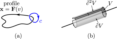
Figure -58: (a) The function $\gamma$ has a monodromy as one goes around the cycle $c$ that links with the profile. (b) The integral region in Eq. (3.9). The contribution from the top and bottom surfaces of the tube is negligible if the tube is very thin.

The integrability condition (2.20) requires

$$V{\bigtriangleup}M-M{\bigtriangleup}V+\frac{1}{2}\left(K^{I}{\bigtriangleup}L_{I}-L_{I}{\bigtriangleup}K^{I}\right)=-{\bigtriangleup}\gamma\equiv 0\,.$$ (3.8)

Superficially, this is satisfied because $\gamma$ is harmonic. However, one must be careful because $\gamma$ is singular along the profile and may have delta-function source there (as is the case for $L_{1,2}$). We can show that it actually does not even have delta-function source as follows. If we integrate ${\bigtriangleup}\gamma$ over a small tubular volume $V$ containing the profile ${\mathbf{x}}={\mathbf{F}}(\lambda)$, we get

$$\int_{V}d^{3}x\,\,{\bigtriangleup}\gamma=\int_{V}d{*_{3}d\gamma}=\int_{\partial V}*_{3}d\gamma=\int_{\partial V}d\alpha=\int_{\partial^{2}V}\alpha=0\,,$$ (3.9)

where the last equality holds because $\alpha$ is single-valued. See Fig. -58(b) for explanation of the integral region. Therefore, ${\bigtriangleup}\gamma$ in (3.8) vanishes everywhere, even on the profile, and the integrability condition is satisfied for any profile ${\mathbf{F}}(\lambda)$.

From harmonic functions (3.1), we can read off various functions and forms that appear in the full solution:

$$Z_{1}=f_{2}\,,\quad Z_{2}=f_{1}\,,\quad Z_{3}=1\,,\quad\mu=0\,,\quad\omega=-\alpha\,,\quad\xi^{1}=\xi^{2}=0\,,\quad\xi^{3}=-\alpha\,.$$ (3.10)

The existence of $\omega$ is guaranteed by the integrability condition. Substituting this data into (2.23), we obtain the type IIA fields:

$$\begin{split}ds_{10}^{2}&=-(f_{1}f_{2})^{-1/2}(dt-\alpha)^{2}+(f_{1}f_{2})^{1/2}dx^{i}dx^{i}\\ &\qquad+(f_{1}/f_{2})^{1/2}dx_{45}^{2}+(f_{2}/f_{1})^{1/2}dx_{67}^{2}+(f_{1}f_{2})^{1/2}dx_{89}^{2}\,,\\ e^{2\Phi}&=(f_{1}f_{2})^{1/2}\,,\qquad B_{2}=\gamma\,dx^{8}\wedge dx^{9}\,,\\ C_{1}&=0\,,\qquad C_{3}=-f_{2}^{-1}(dt-\alpha)\wedge dx^{4}\wedge dx^{5}-f_{1}^{-1}(dt-\alpha)\wedge dx^{6}\wedge dx^{7}\,,\\ \end{split}$$ (3.11)

where we have dropped some total derivative terms in the RR potentials. Since $f_{1},f_{2}\to 1$ as $|{\mathbf{x}}|\to\infty$, the spacetime is asymptotically ${\mathbb{R}}^{1,3}\times T^{6}$. Multi-valuedness is restricted to the $B$-field and the metric is single-valued; namely, this solution is geometric.

One can show that the solution (3.11) has the expected monopole charge; it has monopole charge for D2(67) and D2(45) but not for NS5 (we show this for more general solutions in the next subsection). The dipole charge for NS5 is easier to see in the monodromy of the Kähler moduli, as we discussed around (2.31), and their values are

$$\tau^{1}=i\frac{R_{4}R_{5}}{l_{s}^{2}}\sqrt{f_{1}\over f_{2}}\,,\qquad\tau^{2}=i\frac{R_{6}R_{7}}{l_{s}^{2}}\sqrt{f_{2}\over f_{1}}\,,\qquad\tau^{3}=\frac{R_{8}R_{9}}{l_{s}^{2}}\left(\gamma+i\sqrt{f_{1}f_{2}}\right)\,.$$ (3.12)

$\tau^{1}$ and $\tau^{2}$ are single-valued while, as we can see from (3.7), $\tau^{3}$ has the following monodromy as we go around the supertube along cycle $c$:

$$\tau^{3}\to\tau^{3}+1\,,$$ (3.13)

where we used (3.4) and (3.7). This is the correct monodromy around an NS5-brane. So, this solution has the expected monopole and dipole charge.

Although we have derived the harmonic functions (3.1) by dualizing known solutions, we can also derive it by requiring that they represent the charge and dipole charge expected of the supertube (1.2) as follows. First, no D6-brane means $V=1$ and no D0-brane means $\mu=0$. Then (2.23) implies that, in order to have an NS5-brane along the profile ${\mathbf{F}}(\lambda)$, the harmonic function $K^{3}\equiv\gamma$ must have the monodromy (3.7). As we show in Appendix B, this means that $\gamma$ must be given in terms of $\alpha$ via (3.5) and (3.6). Next, to account for the D2 charges dissolved in the NS5 worldvolume, we need $L_{1},L_{2}$ given in (3.1) and (3.2).

Note that, if we lift the supertube (1.2) to M-theory, we have

$$\mathrm{M2(67)+M2(45)\to m5(\lambda 4567)}\,.$$ (3.14)

Therefore, our solution simply corresponds to the 4D version of Bena and Warner’s solution in [7]. The difference is that they were discussing 5D solutions with general supertube shapes, while we are focusing on solutions which has an isometry and can be reduced to 4D. Because of that, we can be more explicit in the solution in terms of harmonic functions.

D2(89)+D6(456789)$\to 5_{2}^{2}(\lambda$4567;89)

The second example is the $\rm D2+D6\to 5^{2}_{2}$ supertube (1.3), which can be obtained by taking the $T$-dual of the above solution (3.11) along 6789 directions. Involving the exotic $5^{2}_{2}$-brane, this is a non-geometric supertube where the metric becomes multi-valued.

Harmonic functions which describe this supertube (1.3) are

$$V =f_{2}\,,\quad K^{1} =\gamma\,, K^{2} =\gamma\,, K^{3} =0\,,$$ (3.15)

$$L_{1} =1\,, L_{2} =1\,, L_{3} =f_{1}\,, \quad M =0\,.$$

The charges appearing in harmonic functions are related to brane numbers by

$$Q_{1}=\frac{g_{s}l_{s}^{5}}{2R_{4}R_{5}R_{6}R_{7}}N_{1}\,,\qquad Q_{2}=\frac{g_{s}l_{s}}{2}N_{2}\,,\qquad L=\frac{2\pi g_{s}l_{s}^{7}}{R_{4}R_{5}R_{6}R_{7}R_{8}R_{9}}N_{1}\,.$$ (3.16)

As we can easily check, the integrability condition (2.20) is trivially satisfied. The various functions and forms are

$$Z_{1}=Z_{2}=1\,,\quad Z_{3}=f_{1}F\,,\quad\xi^{1}=\xi^{2}=-\alpha\,,\quad\xi^{3}=0\,,\quad\mu=f_{2}^{-1}\gamma\,,\quad\omega=-\alpha\,.$$ (3.17)

The IIA fields are given by

$$\begin{split}ds_{10}^{2}&=-(f_{1}f_{2})^{-1/2}(dt-\alpha)^{2}+(f_{1}f_{2})^{1/2}dx^{i}dx^{i}+(f_{1}/f_{2})^{1/2}\left(dx_{4567}^{2}+f_{1}^{-1}F^{-1}dx_{89}^{2}\right)\,,\\ e^{2\Phi}&=f_{1}^{1/2}f_{2}^{-3/2}F^{-1}\,,\qquad B_{2}=-\frac{\gamma}{f_{1}f_{2}F}\,dx^{8}\wedge dx^{9},\\ C_{1}&=\beta_{2}-f_{1}^{-1}\gamma\,(dt-\alpha)\,,\\ C_{3}&=-\frac{1}{f_{1}F}(dt-\alpha)\wedge dx^{8}\wedge dx^{9}-\frac{\gamma}{f_{1}f_{2}F}\,\beta_{2}\wedge dx^{8}\wedge dx^{9}\,,\end{split}$$ (3.18)

where we defined

$$F\equiv 1+\frac{\gamma^{2}}{f_{1}f_{2}}\,.$$ (3.19)

We have dropped some total derivative terms in the RR potentials. Since $f_{1},f_{2}\to 1$ as $|{\mathbf{x}}|\to\infty$, the spacetime is asymptotically ${\mathbb{R}}^{1,3}\times T^{6}$. However, because the multi-valued function $\gamma$ enters the metric, this spacetime is non-geometric. Every time one goes through the supertube, one goes to different spacetime with different radii for $T^{2}_{89}$, although it is related to the original one by $T$-duality.

It is not difficult to show that the solution (3.18) carries the expected monopole charge for D2(89) and D6(456789), and not for other charges. To see the $5^{2}_{2}$ dipole charge, let us look at the Kähler moduli which are

$$\tau^{1}=i\frac{R_{4}R_{5}}{l_{s}^{2}}\sqrt{\frac{f_{1}}{f_{2}}}\,,\quad\tau^{2}=i\frac{R_{6}R_{7}}{l_{s}^{2}}\sqrt{\frac{f_{1}}{f_{2}}}\,,\quad\tau^{3}=\frac{R_{8}R_{9}}{l_{s}^{2}}\left(-\frac{\gamma}{f_{1}f_{2}F}+i\frac{1}{\sqrt{f_{1}f_{2}}F}\right)\,.$$ (3.20)

If we define

$$\tau^{\prime 3}\equiv-\frac{1}{\tau^{3}}=\frac{l_{s}^{2}}{R_{8}R_{9}}\left(\gamma+i\sqrt{f_{1}f_{2}}\right)\,,$$ (3.21)

the monodromy around the supertube is simply

$$\tau^{\prime 3}\to\tau^{\prime 3}+1\,,$$ (3.22)

where we used (3.7) and (3.16). This is the correct monodromy for the $5^{2}_{2}$-brane.

Although one sees that the RR potentials are also multi-valued in (3.18), this does not mean that we have further monopole or dipole charges. We will see this in a different example in subsection 3.2.

Other duality frames

One can also consider supertube transitions in other duality frames, such as

$$\rm D0+D4(4567)\to ns5(\lambda 4567)$$ (3.23)

or

$$\rm D4(6789)+D4(4589)\to 5^{2}_{2}(\lambda 4567,89)\,.$$ (3.24)

The latter transition (3.24) was studied in [3, 4]. The configuration on the left hand side of (3.23) and (3.24) are not in the timelike class but in the null class [6, 8], and their analysis requires a different 5D ansatz from the one we used above.

3.2 2-dipole solutions

A naive attempt

In the above, we demonstrated how the codimension-2 solution with one dipole charge fits into the 4D/5D solution. The next step is to combine two such solutions so that there are two different types of dipole charge. For example, can we construct a solution in which the supertube transition (1.2) happens simultaneously for two different D2-D2 pairs? For example, consider

$$\begin{array}[]{lclcl}\mathrm{D2(45)}&+&\mathrm{D2(89)}&\to&\mathrm{ns5(\lambda 4589)}\\ \mathrm{D2(67)}&+&\mathrm{D2(89)}&\to&\mathrm{ns5(\lambda 6789)}\end{array}\,.$$ (3.25)

How can we construct harmonic functions corresponding to this configuration? For codimension-3 solutions (2.25), having multiple centers was achieved just by summing the harmonic functions for each individual center. So, a naive guess is to simply sum the harmonic functions for each individual supertube, as follows:

$$V =1\,,\quad K^{1} =\gamma^{\prime}\,, K^{2} =\gamma\,, K^{3} =0\,,$$ (3.26)

$$L_{1} =f_{1}\,, L_{2} =f_{1}^{\prime}\,, L_{3} =f_{2}+f_{2}^{\prime}\,, \quad M =-\frac{\gamma}{2}-\frac{\gamma^{\prime}}{2}\,.$$

However, this does not work; as one can easily check, the integrability condition (2.20) is not generally satisfied for this ansatz (3.26). The two dipoles talk to each other and we must appropriately modify the harmonic functions to construct a genuine solution.

A non-trivial 2-dipole solution

So, the above naive attempt does not work and we must take a different route to find a 2-dipole solution. Here, we use the superthread (or supersheet) solution of [54] to construct one. The superthread solution describes a system of D1 and D5-branes with traveling waves on them, and corresponds to the following simultaneous supertube transitions:

$$\begin{array}[]{lclcl}\mathrm{D1(5)}&+&\mathrm{P(5)}&\to&\mathrm{d1(\lambda)}\\ \mathrm{D5(56789)}&+&\mathrm{P(5)}&\to&\mathrm{d5(\lambda 6789)}\end{array}\,.$$ (3.27)

The left hand side of (3.27) can be thought of as the constituents of the 3-charge black hole. This is not just a trivial superposition of D1-P and D5-P supertubes, since the two supertubes interact with each other.

The superthread solution was originally obtained as a BPS solution in 6D supergravity. The BPS equations in 6D have a linear structure [55] which descends to that of the 5D equations (2.6) and facilitates the construction of explicit solutions. The 6D BPS equations involve a lightlike coordinate $v$ and a 4-dimensional base space which is flat $\mathbb{R}^{4}$ for the superthreads. We use $\vec{x}=(x^{1},x^{2},x^{3},x^{4})$ for the coordinates of ${\mathbb{R}}^{4}$. The superthread solution is characterized by profile functions $\vec{F}_{p}(v)$, which describe the fluctuation of the D1 and D5-brane worldvolume. The index $p=1,\cdots,n$ labels different threads of the D1-D5 supertubes. We review the superthread solution in Appendix C.

If we smear the superthread solution along $x^{4}$ and $v$ directions, it describes the D1-D5-P supertube (3.27) extending along the ${\mathbb{R}}^{3}_{123}$ directions and can be connected to the 4D/5D solutions discussed in section 2.1. After duality transformations, the resulting solution can be regarded as describing precisely the 2-dipole configuration (3.25). More precisely, the final configuration is as follows. We have $n$ supertubes labeled by $p=1,\dots,n$ and the $p$-th tube has the profile ${\mathbf{x}}={\mathbf{F}}_{p}(\lambda_{p})\in{\mathbb{R}}^{3}$, where $\lambda_{p}$ parametrizes the profile and the function ${\mathbf{F}}_{p}$ has the periodicity ${\mathbf{F}}_{p}(\lambda_{p}+L_{p})={\mathbf{F}}_{p}(\lambda_{p})$. The $p$-th tube carries the D2(45), D2(67), D2(89) monopole charges $Q_{p1},Q_{p2},Q_{p3}$ respectively, as well as ns5 dipole charges displayed in (3.25).

Explicitly, the harmonic functions describing the 2-dipole configuration (3.25) are

$$V =1\,,\qquad K^{1}=\gamma_{2}\,,\quad K^{2}=\gamma_{1}\,,\quad K^{3}=0\,,$$ (3.28a)

$$L_{I} =1+\sum_{p}{Q_{pI}}\int_{p}\frac{1}{R_{p}}=Z_{I}\,,\qquad I=1,2\,,$$ (3.28b)

$$L_{3} =1+\sum_{p}\int_{p}\frac{\rho_{p}}{R_{p}}$$

$$\qquad+\sum_{p,q}{Q_{pq}}\iint_{p,q}\left[\frac{\dot{\mathbf{F}}_{p}\cdot\dot{\mathbf{F}}_{q}}{2R_{p}R_{q}}-\frac{\dot{F}_{pi}\dot{F}_{qj}(R_{pi}R_{qj}-R_{pj}R_{qi})}{F_{pq}R_{p}R_{q}(F_{pq}+R_{p}+R_{q})}\right]-K^{1}K^{2}\,,$$ (3.28c)

$$M ={1\over 2}\sum_{p,q}{Q_{pq}}\iint_{p,q}\frac{\epsilon_{ijk}\dot{F}_{pqi}R_{pj}R_{qk}}{F_{pq}R_{p}R_{q}(F_{pq}+R_{p}+R_{q})}-\frac{1}{2}(K^{1}L_{1}+K^{2}L_{2})$$ (3.28d)

where we defined

$$\begin{split}{\mathbf{R}}_{p}(\lambda_{p})&\equiv\mathbf{x}-\mathbf{F}_{p}(\lambda_{p})\,,\qquad{\mathbf{F}}_{pq}(\lambda_{p},\lambda_{q})\equiv\mathbf{F}_{p}(\lambda_{p})-\mathbf{F}_{q}(\lambda_{q})\,,\\ R_{p}&\equiv\lvert{\mathbf{R}}_{p}\rvert\,,\qquad F_{pq}\equiv\lvert{\mathbf{F}}_{pq}\rvert\,,\qquad\qquad Q_{pq}\equiv Q_{p1}Q_{q2}+Q_{p2}Q_{q1}\,.\end{split}$$ (3.29)

Also, for integrals along the supertubes, we defined

$$\int_{p}\equiv\frac{1}{L_{p}}\int_{0}^{L_{p}}d\lambda_{p}\,,\qquad\iint_{p,q}\equiv\frac{1}{L_{p}L_{q}}\int_{0}^{L_{p}}d\lambda_{p}\int_{0}^{L_{q}}d\lambda_{q}$$ (3.30)

and the dependence on the parameter $\lambda_{p}$ in (3.28) has been suppressed. The quantity $\rho_{p}(\lambda_{p})$ in (3.28c) is an arbitrary function corresponding to the D2(89) density along the $p$-th tube. A similar density could be introduced for $M$ in (3.28d), but it had been ruled out by a no-CTC (closed timelike curve) analysis in [54] and was not included here. The scalars $\gamma_{I}$ satisfy

$$d\gamma_{I}=*_{3}d\alpha_{I}\,,\qquad\alpha_{I}=\sum_{p}Q_{pI}\int_{p}\frac{\dot{{\mathbf{F}}}_{p}\cdot d{\mathbf{x}}}{R_{p}}\,,\qquad I=1,2\,,$$ (3.31)

generalizing (3.5), (3.6). Furthermore, the 1-form $\omega$ is given by

$$\omega =\omega_{0}+\omega_{1}+\omega_{2}\,,$$ (3.32a)

$$\omega_{0} =\sum_{p}(Q_{p1}+Q_{p2})\int_{p}{\dot{{\mathbf{F}}}_{p}\cdot d{\mathbf{x}}\over R_{p}}\,,\qquad\omega_{1}={1\over 2}\sum_{p,q}Q_{pq}\iint_{p,q}{\dot{{\mathbf{F}}}_{p}\cdot d{\mathbf{x}}\over R_{p}R_{q}}\,,$$ (3.32b)

$$\omega_{2} ={1\over 4}\sum_{p,q}Q_{pq}\iint_{p,q}{\dot{F}_{pqi}\over F_{pq}}\Biggl{[}\left({1\over R_{p}}-{1\over R_{q}}\right)dx^{i}-2{R_{pi}R_{qj}-R_{pj}R_{qi}\over R_{p}R_{q}(F_{pq}+R_{p}+R_{q})}dx^{j}\Biggr{]}.$$ (3.32c)

The charges $Q_{pI},Q_{p3}$ and the profile length $L_{p}$ are related to quantized numbers by

$$\begin{split}Q_{p1}&=\frac{g_{s}l_{s}^{5}}{2R_{6}R_{7}R_{8}R_{9}}N_{p}\,,\qquad Q_{p2}=\frac{g_{s}l_{s}^{5}}{2R_{4}R_{5}R_{8}R_{9}}N_{p}\,,\\ Q_{p3}&=\frac{g_{s}l_{s}^{5}}{2R_{4}R_{5}R_{6}R_{7}}N_{p3}\,,\qquad L_{p}=\frac{2\pi g_{s}l_{s}^{3}}{R_{4}R_{5}}N_{p}\,.\end{split}$$ (3.33)

It is interesting to compare the above harmonic functions (3.28) with the naive guess (3.26). The naive $V,K^{1},K^{2},K^{3},L_{1},L_{2}$ were correct, but $L_{3},M$ needed correction terms proportional to $Q_{pq}$ to be a genuine solution. Since $Q_{pq}$ involves the product of two types of charge (D2(45) and D2(67)) and represents interaction between two different dipoles.

It is not immediately obvious that $L_{3}$ and $M$ in (3.28) are harmonic on $\mathbb{R}^{3}$. One can show that their Laplacian is given by

$${\bigtriangleup}L_{3} =-4\pi\sum_{p}\int_{p}\rho_{p}\,\delta^{3}({\mathbf{x}}-{\mathbf{F}}_{p})-4\pi\sum_{p,q}Q_{pq}\iint_{p,q}{\dot{{\mathbf{F}}}_{p}\cdot\dot{{\mathbf{F}}}_{q}\over F_{pq}}\,\delta^{3}({\mathbf{x}}-{\mathbf{F}}_{p})\,,$$ (3.34)

$${\bigtriangleup}M =-{1\over 2}K^{I}{\bigtriangleup}L_{I}=2\pi\sum_{p}Q_{pI}\int_{p}K^{I}({\mathbf{F}}_{p})\,\delta^{3}({\mathbf{x}}-{\mathbf{F}}_{p})\,.$$ (3.35)

Namely, $L_{3}$ and $M$ are harmonic up to delta-function source along the profile. In deriving these, we used the following relations:

$${\bigtriangleup}\left[\frac{R_{pi}R_{qj}-R_{pj}R_{qi}}{F_{pq}R_{p}R_{q}(F_{pq}+R_{p}+R_{q})}\right]=-\frac{R_{pi}R_{qj}-R_{pj}R_{qi}}{R_{p}^{3}R_{q}^{3}}\,,$$ (3.36)

$$\int_{p}{{\mathbf{R}}_{p}\cdot\dot{{\mathbf{F}}}_{p}\over R_{p}^{3}}=\int_{p}\partial_{\lambda_{p}}\!\!\left({1\over R_{p}}\right)=0\,,\qquad{\bigtriangleup}\!\left({1\over|{\mathbf{x}}|}\right)=-4\pi\delta^{3}({\mathbf{x}})\,.$$ (3.37)

With the relations (3.34) and (3.35), it is straightforward to show that the integrability condition (2.20) is identically satisfied for any profile.

The harmonic functions $L_{3},M$ in (3.28) are multi-valued, because $K^{1},K^{2}$ are. However, the quantities that actually enter the 10D metric (2.23) are single-valued. Indeed,

$$Z_{3} =1+\sum_{p}\int_{p}\frac{\rho_{p}}{R_{p}}+\sum_{p,q}{Q_{pq}}\iint_{p,q}\left[\frac{\dot{\mathbf{F}}_{p}\cdot\dot{\mathbf{F}}_{q}}{2R_{p}R_{q}}-\frac{\dot{F}_{pi}\dot{F}_{qj}(R_{pi}R_{qj}-R_{pj}R_{qi})}{F_{pq}R_{p}R_{q}(F_{pq}+R_{p}+R_{q})}\right]\,,$$ (3.38a)

$$\mu ={1\over 2}\sum_{p,q}{Q_{pq}}\iint_{p,q}\frac{\epsilon_{ijk}\dot{F}_{pqi}R_{pj}R_{qk}}{F_{pq}R_{p}R_{q}(F_{pq}+R_{p}+R_{q})}\,.$$ (3.38b)

So, the metric is single-valued and the spacetime is geometric. This is as it should be because the configuration (3.25) does not contain any non-geometric exotic branes.

Single/multi-valuedness and physical condition

It is instructive to see how these multi-valued harmonic functions come about in solving the BPS equations as reviewed in subsection 2.1. Assume that we are given $V,K^{I}$ of (3.28a) (which corresponds to having specific ns5-brane dipole charges and no D6-brane), and consider finding $L_{I},M$ or equivalently $Z_{I},\mu$ from the BPS equations. To find $Z_{I}$, we must solve (2.14). For $I=1,2$, this gives a simple Laplace equation for $L_{1},L_{2}$, whose solution is (3.28b). On the other hand, the equation (2.14) for $Z_{3}$ reads

$${\bigtriangleup}Z_{3}={\bigtriangleup}(K^{1}K^{2})=2\partial_{i}K^{1}\partial_{i}K^{2}=2(\partial_{i}\alpha_{1j}\partial_{i}\alpha_{2j}-\partial_{i}\alpha_{1j}\partial_{j}\alpha_{2i})\,.$$ (3.39)

Although $K^{1,2}$ are multi-valued, the last expression in (3.39) is a single-valued. Therefore, it is possible to solve this Poisson equation for $Z_{3}$ using the standard Green function $-{1\over 4\pi}{1\over|{\mathbf{x}}-{\mathbf{x}}^{\prime}|}$, and the result will be automatically single-valued. The above solution (3.38a) corresponds to this solution. This is physically the correct solution in the current situation where we only have standard (D2 and NS5) branes and the metric must be single-valued. Alternatively, we can solve (3.39) in terms of a multi-valued function. If we rewrite (3.39) as ${\bigtriangleup}L_{3}=0$ with $L_{3}=Z_{3}-K^{1}K^{2}$, then $L_{3}=1+\sum_{p}\int_{p}(\rho_{p}/R_{p})\equiv L_{3}^{\text{alt}}$ is a possible solution. This is the direct analogue of what we did for the codimension-3 solution. This gives a multi-valued $Z_{3}=L_{3}+K^{1}K^{2}\equiv Z_{3}^{\text{alt}}$ and hence a multi-valued metric, which is physically unacceptable.

One may find it strange that there are two different solutions, $Z_{3}$ of (3.38a) and $Z_{3}^{\text{alt}}$, to the same Poisson equation (3.39). However, the solution to the Poisson equation is unique given the boundary condition at infinity. The two solutions have different boundary conditions (a single-valued one for the $Z_{3}$ of (3.38a) and a multi-valued one for $Z_{3}^{\text{alt}}$) and there is no contradiction that they are both solutions to the same Poisson equation. The BPS equations such as (3.39) must be solved taking into account the physical situation one is considering.

The $\mu$ equation (2.17) is

$${\bigtriangleup}\mu={1\over 2}{\bigtriangleup}(K^{I}L_{I})=\partial_{i}K^{I}\partial_{i}Z_{I}=\epsilon_{ijk}|\epsilon_{IJ}|\partial_{j}\alpha_{Jk}\partial_{i}Z_{I}\,.$$ (3.40)

Again, we have two options. The first one is to use the standard single-valued Green function to the last expression to obtain the single-valued $\mu$ as given in (3.38b). The second one is to rewrite the above as ${\bigtriangleup}M=0$, $M=\mu-(1/2)K^{I}L_{I}$ and say that $M$ is single-valued. This gives multi-valued $\mu$ and is inappropriate for the current situation.

Closed timelike curves

It is known that near an over-rotating supertube there can be closed timelike curves (CTCs) which must be avoided in physically acceptable solutions [52, 54]. The dangerous direction for the CTCs is known to be along the supertube, which is inside ${\mathbb{R}}^{3}$. By setting $dt=d\psi=0$ in the metric (2.3), the line element inside ${\mathbb{R}}^{3}$ is

$$dl^{2}=-Z^{-2/3}(\mu A+\omega)^{2}+Z^{1/3}(V^{-1}A^{2}+Vd{\mathbf{x}}^{2})\,.$$ (3.41)

In the present case, we have $V=1$ and $A=0$, and therefore the line element becomes

$$dl^{2}=Z^{-2/3}(-\omega^{2}+Zd{\mathbf{x}}^{2})\,,$$ (3.42)

where $\omega$ is given by (3.32).

In the near-tube limit in which we approach a particular point ${\mathbf{F}}_{p}(\lambda_{p}^{0})$ on the $p$-th curve, where $\lambda_{p}^{0}$ is the value of the parameter corresponding to that point, the functions $Z_{1,2,3}$ can be expanded as

$$Z_{I} =Q_{pI}{\cal R}+1+c_{I}+\mathcal{O}(r_{\perp})\,,\qquad I=1,2\,,$$ (3.43a)

$$Z_{3} =\left(Q_{p1}\dot{\mathbf{F}}_{p}{\cal R}+\mathbf{d}_{1}+\mathcal{O}(r_{\perp})\right)\left(Q_{p2}\dot{\mathbf{F}}_{p}{\cal R}+\mathbf{d}_{2}+\mathcal{O}(r_{\perp})\right)+\rho_{p}(\lambda_{p}^{0}){\cal R}+c_{3}+1+\mathcal{O}(r_{\perp})$$

$$=Q_{p1}Q_{p2}\lvert\dot{\mathbf{F}}_{p}\rvert^{2}{\cal R}^{2}+\left[\rho_{p}(\lambda_{p}^{0})+\left(Q_{p1}\mathbf{d}_{2}+Q_{p2}\mathbf{d}_{1}\right)\cdot\dot{\mathbf{F}}_{p}\right]{\cal R}+\text{const.}+\mathcal{O}(r_{\perp})\,.$$ (3.43b)

Here, $\dot{\mathbf{F}}_{p}=\dot{\mathbf{F}}_{p}(\lambda_{p}^{0})$ and ${\cal R}$ is defined as

$${\cal R}\equiv\frac{2}{|\dot{\mathbf{F}}_{p}|}\ln\frac{2\lvert\dot{\mathbf{F}}_{p}\rvert}{r_{\perp}}$$ (3.44)

where $r_{\perp}$ is the transverse distance in ${\mathbb{R}}^{3}$ from the point $\mathbf{F}_{p}(\lambda_{p}^{0})$ on the tube. The constants $c_{I=1,2,3}$ and $\mathbf{d}_{I=1,2}$ are defined in appendix D. Similarly, $\omega_{0,1,2}$ are expanded as

$$\omega_{0} =(Q_{p1}+Q_{p2})\left(\dot{\mathbf{F}}_{p}\cdot d\mathbf{x}\right){\cal R}+\left(\mathbf{d}_{1}+\mathbf{d}_{2}\right)\cdot d\mathbf{x}+\mathcal{O}(r_{\perp})\,,$$ (3.45a)

$$\omega_{1} =Q_{p1}Q_{p2}\left(\dot{\mathbf{F}}_{p}\cdot d\mathbf{x}\right){\cal R}^{2}+\frac{{\cal R}}{2}\left[Q_{p1}\left(\mathbf{d}_{2}+c_{2}\dot{\mathbf{F}}_{p}\right)+Q_{p2}\left(\mathbf{d}_{1}+c_{1}\dot{\mathbf{F}}_{p}\right)\right]\cdot d\mathbf{x}+\mathcal{O}(r_{\perp})\,,$$ (3.45b)

$$\omega_{2} =\frac{{\cal R}}{2}\sum_{q(\neq p)}Q_{pq}\int d\lambda_{p}\,\frac{\left(\dot{\mathbf{F}}_{p}(\lambda_{p}^{0})-\dot{\mathbf{F}}_{q}(\lambda_{p})\right)\cdot d\mathbf{x}}{\lvert\mathbf{F}_{p}(\lambda_{p}^{0})-\mathbf{F}_{q}(\lambda_{p})\rvert}+{\cal O}(r_{\perp})\,.$$ (3.45c)

By plugging in the above expressions, the line element (3.42) becomes

$$Z^{2/3}dl^{2} =(Q_{p1}Q_{p2})^{2}{\cal R}^{4}\lvert\dot{\mathbf{F}}_{p}\rvert^{2}\left(d\mathbf{x}^{2}-\frac{\lvert\dot{\mathbf{F}}_{p}\cdot d\mathbf{x}\rvert^{2}}{\lvert\dot{\mathbf{F}}_{p}\rvert^{2}}\right)$$

$$\quad+(Q_{p1}Q_{p2}){\cal R}^{3}\Biggl{[}\rho_{p}(\lambda_{p}^{0})d\mathbf{x}^{2}+\left(\lvert\dot{\mathbf{F}}_{p}\rvert^{2}d\mathbf{x}^{2}-2\lvert\dot{\mathbf{F}}_{p}\cdot d\mathbf{x}\rvert^{2}\right)\left(Q_{p1}\left(1+c_{2}\right)+Q_{p2}\left(1+c_{1}\right)\right)$$

$$\qquad\qquad\qquad\qquad+\dot{\mathbf{F}}_{p}\cdot\left(Q_{p1}\mathbf{d}_{2}+Q_{p2}\mathbf{d}_{1}\right)d\mathbf{x}^{2}\Biggr{]}+\mathcal{O}({\cal R}^{2})\,.$$ (3.46)

For displacement along the tube, $d\mathbf{x}\propto\dot{\mathbf{F}}_{p}$, the leading ${\cal O}({\cal R}^{4})$ term vanishes and the ${\cal O}({\cal R}^{3})$ term gives the leading contribution. If the coefficient of the ${\cal O}({\cal R}^{3})$ term is negative for all $\lambda_{p}^{0}\in[0,L_{p}]$, the cycle along the tube will be a CTC. Conversely, for the absence of CTCs, there must be some value of $\lambda_{p}^{0}$ for which the following inequality is satisfied:

$$\rho_{p}(\lambda_{p}^{0})\geq Q_{p1}\left(\lvert\dot{\mathbf{F}}_{p}\rvert^{2}(1+c_{2})-\dot{\mathbf{F}}_{p}\cdot\mathbf{d}_{2}\right)+Q_{p2}\left(\lvert\dot{\mathbf{F}}_{p}\rvert^{2}(1+c_{1})-\dot{\mathbf{F}}_{p}\cdot\mathbf{d}_{1}\right)\,.$$ (3.47)

This can be written more explicitly, using (D.11) and (D.15), as

$$\rho_{p}(\lambda_{p}^{0})\geq\lvert\dot{\mathbf{F}}_{p}(\lambda_{p}^{0})\rvert^{2}\left(Q_{p1}+Q_{p2}\right)+\sum_{q(\neq p)}Q_{pq}\int d\lambda_{p}\,\frac{\dot{\mathbf{F}}_{p}(\lambda_{p}^{0})\cdot\left(\dot{\mathbf{F}}_{p}(\lambda_{p}^{0})-\dot{\mathbf{F}}_{q}(\lambda_{p})\right)}{\lvert\mathbf{F}_{p}(\lambda_{p}^{0})-\mathbf{F}_{q}(\lambda_{p})\rvert}\,.$$ (3.48)

This is analogous to the no-CTC condition for the superthread solution (Eq. (2.34) in [54]).

Charge and angular momentum

Let us study if the solution above has the expected monopole and dipole charges. In the presence of Chern-Simons interaction, there are multiple notions of charge [56], and here we choose Page charge, which is conserved, localized, quantized, and gauge-invariant under small gauge transformations. Specifically, the D$p$-brane Page charge is defined as [56, 4] (see also Appendices A and E)

$$Q_{\mathrm{D}p}^{\mathrm{Page}}=\frac{1}{(2\pi l_{s})^{7-p}g_{s}}\int_{M^{8-p}}e^{-B_{2}}G=\frac{1}{(2\pi l_{s})^{7-p}g_{s}}\int_{\partial M^{8-p}}e^{-B_{2}}C\,.$$ (3.49)

Here, $M^{8-p}$ is an $(8-p)$-manifold enclosing the D$p$-brane, and $G=\sum_{p}G_{p+1}$, $C=\sum_{p}C_{p}$ with $p$ odd (even) for type IIA (IIB). In the integrand, we must take the part with the appropriate rank from the polyforms $e^{-B_{2}}G$, $e^{-B_{2}}C$. In the second equality, we used the relation (A.4) between $G$ and $C$.

Using the definition above, we can readily calculate Page charges for this 2-dipole solution. For example, the D4(6789)-brane charge, which is expected to vanish, is given by

$$Q_{\mathrm{D4(6789)}}^{\mathrm{Page}} =\frac{1}{(2\pi l_{s})^{3}g_{s}}\int_{S^{2}\times T^{2}_{45}}e^{-B_{2}}G=\frac{1}{(2\pi l_{s})^{3}g_{s}}\int_{\partial S^{2}\times T^{2}_{45}}e^{-B_{2}}C$$

$$=\frac{R_{4}R_{5}}{2\pi l_{s}^{3}g_{s}}\int_{\partial S^{2}}\left\{\left[-{1\over Z_{1}}+{V\mu\over Z-V\mu^{2}}\left({K^{1}\over V}-{\mu\over Z_{1}}\right)\right]\omega+\xi^{1}\right\}\,,$$ (3.50)

where in the last equality we used (E.4). If the surface $S^{2}$ is at infinity enclosing the entire profile, then the function in the $[\cdots]$ above is single-valued. Also, the requirement of integrability (2.20) guarantees that $\omega$ is also single-valued. Therefore, the entire first term in the integrand is single-valued and does not contribute to the integral on $\partial S^{2}$. The only contribution comes from the second term, $\xi_{1}$. Thus we find

$$Q_{\mathrm{D4(6789)}}^{\mathrm{Page}} =\frac{R_{4}R_{5}}{2\pi l_{s}^{3}g_{s}}\int_{\partial S^{2}}\xi^{1}=\frac{R_{4}R_{5}}{2\pi l_{s}^{3}g_{s}}\int_{S^{2}}d\xi^{1}=-\frac{R_{4}R_{5}}{2\pi l_{s}^{3}g_{s}}\int_{S^{2}}*_{3}dK^{1}\,.$$ (3.51)

The integral is equal to $-4\pi$ times the coefficient of $1/r$ in the large $r$ expansion of $K^{1}$. However, $\alpha_{2}={\cal O}(1/r^{2})$ and hence $K^{1}=\gamma_{2}={\cal O}(1/r^{2})$ and the coefficient of the $1/r$ term vanishes. So, we conclude that $Q_{\mathrm{D4(6789)}}^{\mathrm{Page}}=0$, as expected. Similarly, other Page charges are related to the coefficient of the $1/r$ in the large $r$ expansion of the corresponding harmonic function (see Appendix E for the expressions for necessary RR potentials to compute the Page charge). We find that the non-vanishing charges are

$$Q_{\mathrm{D2(45)}}^{\mathrm{Page}} =Q_{\mathrm{D2(67)}}^{\mathrm{Page}}=\sum_{p}N_{p}\,,$$ (3.52)

$$Q_{\mathrm{D2(89)}}^{\mathrm{Page}} =\sum_{p}N_{p3}\,,\qquad Q_{p3}=\int_{p}\rho_{p}\,,$$ (3.53)

where we used (3.33).

It is easy to check that we have appropriate monodromy for ns5($\lambda$4567) and ns5($\lambda$6780). The real part of $\tau^{1,2}$ contain $K^{1,2}$ (2.24) and others are all single-valued. Then we can apply same argument as (3.7). So we obtain

$$\tau^{1}\to\tau^{1}+1\,,\qquad\tau^{2}\to\tau^{2}+1$$ (3.54)

as we go around each tubes. This is proper monodromy for our system.

The angular momentum can be read off from the ADM formula [57]

$$g_{ti}=-\frac{1}{\sqrt{V(Z-V\mu^{2})}}\,\omega_{i}=-2G_{4}{x^{j}J^{ji}\over|{\mathbf{x}}|^{3}}+\cdots$$ (3.55)

where $G_{4}$ is 4-dimensional Newton constant. By expanding $g_{ti}$ to the leading order, we obtain

$$-g_{ti}={x^{j}\over|{\mathbf{x}}|^{3}}\left(\sum_{p}(Q_{p1}+Q_{p2})\int_{p}\dot{F}_{pi}F_{pj}+{1\over 4}\sum_{p,q}Q_{pq}\iint_{p,q}{\dot{F}_{pqi}F_{pqj}-\dot{F}_{pqj}F_{pqi}\over F_{pq}}\right)+{\cal O}\left({1\over|{\mathbf{x}}|^{3}}\right)$$ (3.56)

where we used

$$\frac{1}{R_{p}}=\frac{1}{|{\mathbf{x}}|}+\frac{{\mathbf{x}}\cdot\mathbf{F}_{p}}{|{\mathbf{x}}|^{3}}+\mathcal{O}\left(\frac{1}{|{\mathbf{x}}|^{3}}\right)\,.$$ (3.57)

Therefore the angular momentum of the 2-dipole solution is

$$J^{ji}={1\over 4G_{4}}\left(\sum_{p}(Q_{p1}+Q_{p2})\int_{p}(\dot{F}_{pi}F_{pj}-\dot{F}_{pj}F_{pi})+{1\over 2}\sum_{p,q}Q_{pq}\iint_{p,q}{\dot{F}_{pqi}F_{pqj}-\dot{F}_{pqj}F_{pqi}\over F_{pq}}\right)\,.$$ (3.58)

The second term represents the contribution from the interaction between supertubes.

3.3 3-dipole solutions

We can also consider a 3-dipole configuration as an extension of the 2-dipole configuration (3.25) such as

$$\begin{array}[]{lclcl}\mathrm{D2(45)}&+&\mathrm{D2(89)}&\to&\mathrm{ns5(\lambda 4589)}\\ \mathrm{D2(67)}&+&\mathrm{D2(89)}&\to&\mathrm{ns5(\lambda 6789)}\\ \mathrm{D2(45)}&+&\mathrm{D2(67)}&\to&\mathrm{ns5(\lambda 4567)}\end{array}\,.$$ (3.59)

Because there is no D6-brane, we have $V=1$. How can we find the rest of harmonic functions for this 3-dipole configuration, generalizing the 2-dipole solution?

First, it is natural to guess that the 3-dipole solution has the dipole sources in all $K^{I=1,2,3}$, generalizing the 2-dipole case where $K^{I=1,2}$ had dipole sources. Namely,

$$\alpha^{I} =\sum_{p}Q_{pI}\int_{p}\frac{\dot{\mathbf{F}}_{p}\cdot d\mathbf{x}}{R_{p}}\,,\qquad dK^{I}=*_{3}d\alpha^{I}\,,\qquad I=1,2,3\,.$$ (3.60)

Note that the next layer of equation (2.14) to determine $Z_{I}$ is quadratic in $K^{I}$ and therefore knows only about 2-dipole interactions. So, we can construct $Z_{I}$ the same way as in the 2-dipole case, as follows:

$$Z_{I} =1+\sum_{p}Q_{pI}\int_{p}\frac{\rho_{pI}}{R_{p}}$$

$$\qquad+C_{IJK}\sum_{p,q}Q_{pJ}Q_{qK}\iint_{p,q}\left[\frac{\dot{\mathbf{F}}_{p}\cdot\dot{\mathbf{F}}_{q}}{2R_{p}R_{q}}-\frac{\dot{F}_{pi}\dot{F}_{qj}(R_{pi}R_{qj}-R_{pj}R_{qi})}{F_{pq}R_{p}R_{q}(F_{pq}+R_{p}+R_{q})}\right]\,,$$ (3.61)

where $I=1,2,3$ and the same shorthand notation (3.29) is used. Finally, the last layer of equation (2.17) to determine $\mu$ is

$${\bigtriangleup}\mu=\partial_{i}Z_{I}\partial_{i}K^{I}=\epsilon_{ijk}\partial_{i}Z_{I}\partial_{j}\alpha_{k}^{I}\,.$$ (3.62)

Because $Z_{I}$ involves 2-dipole interactions, $\mu$ involves 3-dipole interactions. Although we have not been able to solve this in terms of integrals along the tubes as in the 2-dipole case (cf. (3.38b)), we know physically that the solution must be single-valued and therefore we can solve it by using the standard single-valued Green function. Namely, the solution is

$$\mu({\mathbf{x}})=-\frac{1}{4\pi}\int d^{3}x^{\prime}\,\frac{\partial_{i}Z_{I}\partial_{i}K^{I}(\mathbf{x^{\prime}})}{|\mathbf{x}-\mathbf{x^{\prime}}|}\,.$$ (3.63)

In order to satisfy the integrability condition (2.20), we have no option of adding to this a term like $\sum_{p}\int_{p}\sigma_{p}/R_{p}$ with an arbitrary function $\sigma_{p}$, as we did in the second term of (3.38a). In the present case, with $V=1$, ${\bigtriangleup}K^{I}=0$, the integrability condition (2.20) becomes

$$0 =V{\bigtriangleup}M-M{\bigtriangleup}V+\frac{1}{2}\left(K^{I}{\bigtriangleup}L_{I}-L_{I}{\bigtriangleup}K^{I}\right)$$

$$={\bigtriangleup}M+\frac{1}{2}K^{I}{\bigtriangleup}L_{I}={\bigtriangleup}\mu-\partial_{i}Z_{I}\partial_{i}K^{I},$$ (3.64)

where in the last equality we used (2.15), (2.18). This is nothing but (3.62). If we added the term $\sum_{p}\int_{p}\sigma_{p}/R_{p}$ to the $\mu$ in (3.63), then the integrability condition would be violated by a delta-function term. This is why we do not have an option of adding such a term. This also explains as a corollary why we do not have a term like $\sum_{p}\int_{p}\sigma_{p}/R_{p}$ in the 2-dipole $\mu$ in (3.38b).

Although it is not as explicit as the 2-dipole case, (3.63) gives the interacting 3-dipole solution in principle.

4 Mixed configurations

Thus far, we have studied the 4D/5D solution with codimension-2 centers. In this section, we present a simple example in which codimension-3 and codimension-2 centers coexist.

As the simplest codimension-2 center, let us consider the 1-dipole configuration with the harmonic functions (3.1),

$$V =1\,,\quad K^{1} =0\,, K^{2} =0\,, K^{3} =\gamma\,,$$ (4.1)

$$L_{1} =1+f_{2}\,, L_{2} =1+f_{1}\,, L_{3} =1\,, \quad M =-\frac{\gamma}{2}\,,$$

where we have extracted “1” as compared from (3.2) and

$$f_{1} ={Q_{1}\over L}\int_{0}^{L}{d\lambda\over|{\mathbf{x}}-{\mathbf{F}}(\lambda)|}\,,\qquad f_{2}={Q_{1}\over L}\int_{0}^{L}{|\dot{\mathbf{F}}(\lambda)|^{2}d\lambda\over|{\mathbf{x}}-{\mathbf{F}}(\lambda)|}\,,$$ (4.2)

while $\gamma$ is still given by (3.5) and (3.6).

We would like to add to this a codimension-3 source of the type (2.25). Here, let us simply add a codimension-3 singularity to (4.1) as follows:

$$V =n_{0}+{n\over r}\,,$$ (4.3)

$$K^{1} =k^{1}_{0}+{k^{1}\over r}\,, K^{2} =k^{2}_{0}+{k^{2}\over r}\,, K^{3} =k^{3}_{0}+\gamma+{k^{3}\over r}\,,$$

$$L_{1} =l_{1}^{0}+f_{2}+{l_{1}\over r}\,, L_{2} =l_{2}^{0}+f_{1}+{l_{2}\over r}\,, L_{3} =l_{3}^{0}+{l_{3}\over r}\,,$$

$$M =m_{0}-{\gamma\over 2}+{m\over r}\,.$$

For these harmonic functions, the integrability condition (2.20) becomes

$$0 =-4\pi\delta({\mathbf{x}})\left[n_{0}m-m_{0}n+{1\over 2}(k_{0}^{I}l_{I}-l_{I}^{0}k^{I})-{1\over 2}\Bigl{(}k^{1}f_{2}({\mathbf{x}}=0)+k^{2}f_{1}({\mathbf{x}}=0)\Bigr{)}\right]$$

$$\quad-2\pi\gamma\,\delta({\mathbf{x}})(n+l_{3})$$

$$\quad+{1\over 2}\left[\left(k_{0}^{2}+{k^{2}\over r}\right){\bigtriangleup}f_{1}+\left(k_{0}^{1}+{k^{1}\over r}\right){\bigtriangleup}f_{2}\right]\,.$$ (4.4)

The three lines on the right hand side are of different nature and must vanish separately. So,

$$0 =n_{0}m-m_{0}n+{1\over 2}(k_{0}^{I}l_{I}-l_{I}^{0}k^{I})-{1\over 2}{Q\over L}\int_{0}^{L}{d\lambda}{k^{1}|\dot{{\mathbf{F}}}(\lambda)|^{2}+k^{2}\over|{\mathbf{F}}(\lambda)|}\,,$$ (4.5a)

$$0 =n+l_{3}\,,$$ (4.5b)

$$0 =k_{0}^{2}+{k^{2}\over|{\mathbf{F}}(\lambda)|}+|\dot{{\mathbf{F}}}(\lambda)|^{2}\left(k_{0}^{1}+{k^{1}\over|{\mathbf{F}}(\lambda)|}\right)\qquad\text{for each value of $\lambda$.}$$ (4.5c)

The first equation (4.5a) says that the total force exerted by the tube on the $r=0$ brane must vanish. This is a single equation and easy to satisfy. The second equation is also easy to satisfy. On the other hand, the third equation (4.5c) says that the force exerted by the $r=0$ brane on every point of the tube must vanish, and gives the most stringent condition. Let us investigate this last condition in detail.

Note that, if the asymptotic moduli $k_{0}^{1},k_{0}^{2}$ vanished, then the distance between the tube and the codimension-3 brane, $|{\mathbf{F}}(\lambda)|$, would disappear from the condition (4.5c), and we have

$$0 ={k^{2}}+|\dot{{\mathbf{F}}}(\lambda)|^{2}{k^{1}}\,.$$ (4.6)

Because $|\dot{{\mathbf{F}}}(\lambda)|^{2}$ is the ratio of the D2(67) and D2(45) charge densities carried by the tube while $k^{1},k^{2}$ are the D4(6789), D4(4589) charges of the $r=0$ brane, Eq. (4.6) would mean that the tube must have, at every point along it, charge density that would be mutually supersymmetric with the $r=0$ brane in flat space. This can of course happen only if the total charge of the tube is mutually supersymmetric with the $r=0$ brane. In this case, the distance between the two objects is arbitrary, implying that they are not bound.

On the other hand, if the asymptotic moduli $k_{0}^{1},k_{0}^{2}$ are non-vanishing, the tube does not have charge density that would be mutually BPS with the $r=0$ brane in flat space, and the configuration represents a true bound state. The condition (4.5c) gives

$$|\dot{{\mathbf{F}}}(\lambda)|^{2}=-{k_{0}^{2}|{\mathbf{F}}(\lambda)|+k^{2}\over k_{0}^{1}|{\mathbf{F}}(\lambda)|+k^{1}}\,.$$ (4.7)

Because ${\mathbf{F}}(\lambda)$ is a vector with three components, this differential equation leaves the orientation of $\dot{{\mathbf{F}}}(\lambda)$ undetermined. Therefore, the tube profile can wiggle depending on two functions of one variable. We expect that this remains true for more general configurations with both codimension-2 and codimension-3 centers: each codimension-2 center has a profile depending on two functions of one variable, so that the force from other centers vanishes at each point along the tube.

5 Discussion

In this paper, we studied the BPS configurations of the brane system in string theory in the framework of 5D supergravity. In the literature, multi-center configurations of codimension-3 branes have been extensively studied. However, we pointed out that these codimension-3 branes can polarize into codimension-2 ones by the supertube effect and hence multi-center configurations involving codimension-2 branes along arbitrary curves must also be included if we want to capture the full configuration space of the system. Codimension-2 branes can be exotic, and the solution containing them can represent non-geometric spacetime.

Therefore, the most general configuration is a multi-center configuration including both codimension-3 branes and codimension-2 ones. In the framework of the 4D/5D solution, such configurations are described by harmonic functions with codimension-3 and codimension-2 singularities in ${\mathbb{R}}^{3}$. In this paper, we provided some simple examples of such solutions, hoping that they serve as a guide for constructing general solutions.

The solutions with codimension-2 centers have various possible applications and implications, some of them already mentioned in the Introduction. Here let us discuss their relevance to the fuzzball proposal for black holes [28, 58, 59, 60, 61] and the microstate geometry program.

Smooth 4D/5D solutions with codimension-3 centers have been put forward as possible microstates for the 3- and 4-charge black holes [26, 27]. However, the entropy represented by these solutions have been estimated [62, 63] to be parametrically smaller than the entropy of the corresponding black hole. In particular, for the 3-charge black hole, Ref. [63] considered placing a probe supertube in the scaling geometry [64, 65] and estimated the associated entropy to be $\sim Q^{5/4}$ whereas the desired black hole entropy is $\sim Q^{3/2}$, where $Q\sim Q_{1,2,3}$ is the charge of the black hole. In our setup, a supertube in a scaling geometry corresponds to a configuration with codimension-3 centers as well as a codimension-2 one. It may be possible to make their estimate more precise by including backreaction using our setup.

Another issue with identifying smooth 4D/5D solutions with codimension-3 centers with black hole microstates concerns the pure Higgs branch. Ref. [66] (see also [67]) studied quiver quantum mechanics describing 3-center solutions and showed that most entropy of the system comes from zero-angular momentum states in what they call the pure Higgs branch. On the other hand, the multi-center solutions with codimension-3 centers are naturally identified with states in the Coulomb branch of the quiver quantum mechanics. This is because the codimension-3 solutions are characterized by the position of the centers, which corresponds to the adjoint vev in the quiver quantum mechanics. Therefore, these solutions do not seem to correspond to typical microstates of the system. In contrast, a codimension-2 center has a finite-sized profile, as a result of two branes getting bound together and puffing up by the supertube effect. In the quiver quantum mechanics, this has a natural interpretation as a Higgs branch state, with a finite vev for the bifundamental matter connecting two centers or nodes. Therefore, it is very interesting to understand the relation between the codimension-2 configurations in gravity and states in quiver quantum mechanics to elucidate the role of codimension-2 centers in black hole microphysics.

We have focused on codimension-2 centers in this paper but, of course, we could consider objects with still lower codimensions, namely one and zero. A codimension-1 center is a membrane in ${\mathbb{R}}^{3}$ and is a 4D/5D-solution realization of the “superstrata” recently proposed as possible microstates [3, 4, 68, 69]. It is interesting to study if the setup of the 4D/5D solution sheds new light on superstrata or makes their construction and analysis easier. Codimension-1 and codimension-0 branes are generally more non-geometric than the codimension-2 ones [34, 37], and studying them in the context of the 4D/5D solution is an interesting subject.

Explicit construction of a solution with codimension-2 centers with general charge, position and profile is technically a challenging problem. In subsection 3.2, we discussed how to solve the BPS equations of subsection 2.1 for a 2-dipole supertube. As mentioned there, when solving the BPS equations, there are multiple solutions differing in the monodromy properties. We must construct them and choose from them the physically appropriate one expected from the dipole charges produced by supertube transitions. This is in some sense similar to (but more complicated than) the problem of finding solutions of F-theory with various monodromies around 7-branes [1, 2, 70] and is a non-trivial task. In particular, in the presence of non-trivial harmonic function $V$, which corresponds to having D6-branes, solving Eq. (2.14) is itself a challenging problem. We leave this for future research.

To conclude, the solutions involving codimension-2 provide interesting new directions of research, and studying them is bound to reveal richer physics of brane systems than was found in codimension-3 solutions. We hope to report on the progress in such research in near future.

Appendix A Convention

The reduction formulas for the 11D metric and 3-form potential to type IIA supergravity in 10D are

$$\begin{split}ds_{11}^{2}&=e^{-\frac{2}{3}\Phi}ds_{\mathrm{10,str}}^{2}+e^{\frac{4}{3}\Phi}\left(dx^{11}+C_{1}\right)^{2}\,,\\ {\cal A}_{3}&=C_{3}+B_{2}\wedge dx^{11}\,.\end{split}$$ (A.1)

The relation between the gauge-invariant RR field strength $G_{p+2}$ and the RR potential $C_{p+1}$ is

$$G_{p+2}=dC_{p+1}-H_{3}\wedge C_{p-1}\,,$$ (A.2)

where $H_{3}=dB_{2}$. The higher forms $G_{6},G_{8}$ are related to $G_{4},G_{2}$ by

$$G_{6}=*G_{4}\,,\qquad G_{8}=-*G_{2}\,.$$ (A.3)

If we define the polyforms $G=\sum_{p}G_{p+1}$, $C=\sum_{p}C_{p}$ with $p$ odd (even) for type IIA (IIB), the relation (A.2) can be written more concisely as

$$G=dC-H_{3}\wedge C=e^{B_{2}}d(e^{-B_{2}}C)\,.$$ (A.4)

We define the Hodge dual of a $p$-form $\omega$ in $d$ dimensions as

$$(*\,\omega)_{i_{1}\cdots i_{d-p}} =\frac{1}{p!}\,\epsilon_{i_{1}\cdots i_{d-p}}{}^{j_{1}\cdots j_{p}}\omega_{j_{1}\cdots j_{p}}\,,$$ (A.5)

$$*(dx^{j_{1}}\wedge\cdots\wedge dx^{j_{p}}) =\frac{1}{(d-p)!}\,dx^{i_{1}}\wedge\cdots\wedge dx^{i_{d-p}}\epsilon_{i_{1}\cdots i_{d-p}}{}^{j_{1}\cdots j_{p}}\,,$$ (A.6)

with

$$\epsilon_{01\dots(d-1)}=-\sqrt{-g}\,,\qquad\epsilon^{01\dots(d-1)}=+{1\over\sqrt{-g}}\,.$$ (A.7)

Appendix B Monodromic harmonic function

Here, we show that if the harmonic function $\gamma$ has the monodromy (3.7) independent of the cycle $c$, then it is given in terms of the 1-form $\alpha$ by (3.5) and (3.6).

Harmonicity of $\gamma$ means that $d(*_{3}d\gamma)=0$, which implies that $*_{3}d\gamma$ is closed and can be written in terms of a 1-form $\alpha$ as $*_{3}d\gamma=d\alpha$ at least locally. Because $\alpha$ has the gauge ambiguity $\alpha\to\alpha+d\Lambda$ where $\Lambda$ is a scalar, we can impose the “Lorenz gauge” $\partial_{i}\alpha_{i}=0$. In this gauge, the monodromy of $\gamma$ can be expressed as

$$\Delta\gamma=\int_{c}d\gamma=\int_{c}*_{3}d\alpha=\int_{D}d*_{3}d\alpha=-\int_{D}{\bigtriangleup}\alpha_{i}\,{1\over 2}\epsilon_{ijk}dx^{j}\wedge dx^{k}=-\int_{D}{\bigtriangleup}\alpha_{i}\,n_{i}\,d^{2}\!A\,,$$ (B.1)

where $D$ is a 2-surface with $\partial D=c$, $n_{i}$ is the unit normal to $D$, and $d^{2}\!A$ is the area element of $D$. In order for the monodromy $\Delta\gamma$ not to change even if we homotopically deform the cycle $c$, the quantity ${\bigtriangleup}\alpha$ can only have delta-function source along the profile ${\mathbf{x}}={\mathbf{F}}(\lambda)$. Therefore, it must be that

$$\alpha_{i}({\mathbf{x}})={1\over L}\int_{0}^{L}{v_{i}(\lambda)\over|{\mathbf{x}}-{\mathbf{F}}(\lambda)|}d\lambda$$ (B.2)

where $v_{i}(\lambda)$ are some functions. This gives

$${\bigtriangleup}\alpha_{i}({\mathbf{x}})=-{4\pi\over L}\int_{0}^{L}v_{i}(\lambda)\,\delta^{2}({\mathbf{x}}-{\mathbf{F}}(\lambda))\,d\lambda\,.$$ (B.3)

Namely, $\alpha_{i}$ has delta-function source distributed along the profile with (vectorial) density $v_{i}$. Then (B.1) is proportional to

$$v_{i}n_{i}\times{1\over\cos\theta}\times{1\over|\dot{{\mathbf{F}}}|}\,,$$ (B.4)

where $\theta$ is the angle between $n_{i}$ and the unit tangent to the profile, $t_{i}$. The second factor takes into account the fact that the curve does not necessarily perpendicularly intersect with $D$, and the third factor takes into account the “speed” of the parametrization $\lambda$. Because $\cos\theta=t_{j}n_{j}$ and $t_{j}=\dot{F}_{j}/|\dot{{\mathbf{F}}}|$, the quantity (B.4) is equal to

$${v_{i}n_{i}\over t_{j}n_{j}}\,.$$ (B.5)

Given $c$, there are infinitely many choices for $D$ which can intersect the profile at any point at any angle. So, if (B.5) is to be independent of the choice of $D$, the only possibility is $v_{i}\propto\dot{F}_{i}$. This means that $\alpha$ is given by (3.6).

Appendix C Superthread

In this Appendix, we briefly review the superthread solution which was used in subsection 3.2 to derive the 2-dipole solution. The superthread solution was originally obtained in [54] as a BPS solution in 6D supergravity [55].

The metric for the superthread is

$$ds_{6}^{2}=2(Z_{1}Z_{2})^{-1/2}dv\left(du+k+\frac{1}{2}\mathcal{F}\,dv\right)-(Z_{1}Z_{2})^{1/2}ds_{4}^{2}$$ (C.1)

where the base space is flat ${\mathbb{R}}^{4}$ with metric $ds_{4}^{2}=\delta_{ij}dx^{i}dx^{j}$ ($i=1,\cdots,4$). We denote the coordinates of the ${\mathbb{R}}^{4}$ by $\vec{x}=(x^{1},x^{2},x^{3},x^{4})$. All quantities that appear in the metric are independent of the coordinate $u$. The scalars $Z_{I}$, $I=1,2$ are harmonic functions in $\mathbb{R}^{4}$ and are given by

$$Z_{I}=1+\sum_{p}\frac{Q_{pI}}{R_{p}^{2}}\,,$$ (C.2)

where

$$R_{p}\equiv\lvert\vec{x}-\vec{F}^{(p)}(v)\rvert$$ (C.3)

and $\vec{F}^{(p)}(v)\in{\mathbb{R}}^{4}$ is the profile of the supertube. Note that we use this ${\mathbb{R}}^{4}$ version of $R_{p}$ only in this appendix ($R_{p}$ in the main text is defined for ${\mathbb{R}}^{3}$ as in (3.29)). The 6D solution also involve self-dual field strengths

$$\Theta^{I}=*_{4}\Theta^{I}\,,\quad I=1,2\,,$$ (C.4)

which are related to $Z_{I}$ by the following equation:

$$d\Theta^{I}=|\epsilon^{IJ}|\,{*_{4}d\dot{Z}_{J}}\,.$$ (C.5)

Here $\dot{~{}~{}}$ means the $v$-derivative and $d$ is the exterior derivative with respect to the ${\mathbb{R}}^{4}$. For $Z_{I}$ given in (C.2), this equation can be solved by

$$\Theta^{I}=(1+*_{4})d\left(|\epsilon^{IJ}|\sum_{p}Q_{pJ}\frac{\dot{\vec{F}}^{(p)}\cdot d\vec{x}}{R_{p}^{2}}\right)\,.$$ (C.6)

The 1-form $k$ appearing in the metric (C.1) satisfies the relation

$$(1+*_{4})dk=Z_{I}\Theta^{I}\,.$$ (C.7)

The solution to this equation is

$$k =k_{0}+k_{1}+k_{2}\,,$$ (C.8a)

$$k_{0} =\sum_{I=1,2}\sum_{p}{Q_{pI}\dot{\vec{F}}^{(p)}\cdot d\vec{x}\over R_{p}^{2}}\,,$$ (C.8b)

$$k_{1} ={1\over 2}\sum_{p,q}Q_{pq}{\dot{\vec{F}}^{(q)}\cdot d\vec{x}\over R_{p}^{2}R_{q}^{2}}={1\over 4}\sum_{p,q}Q_{pq}{(\dot{\vec{F}}^{(p)}+\dot{\vec{F}}^{(q)})\cdot d\vec{x}\over R_{p}^{2}R_{q}^{2}}\,,$$ (C.8c)

$$k_{2} ={1\over 4}\sum_{p,q}Q_{pq}{\dot{F}^{(p)}_{i}-\dot{F}^{(q)}_{i}\over\lvert\vec{F}^{(p)}-\vec{F}^{(q)}\rvert^{2}}\left[\left({1\over R_{p}^{2}}-{1\over R_{q}^{2}}\right)dx^{i}-{2\over R_{p}^{2}R_{q}^{2}}{\cal A}_{ij}^{(p,q)}dx^{j}\right]\,,$$ (C.8d)

where we defined

$$Q_{pq}\equiv Q_{p1}Q_{q2}+Q_{q1}Q_{p2}\,.$$ (C.9)

With this $k$, the scalar field $\mathcal{F}$ can be obtained by solving the equation

$$-*_{4}d*_{4}d\mathcal{F}=*_{4}(\Theta^{1}\wedge\Theta^{2})+2\dot{Z_{1}}\dot{Z_{2}}\,.$$ (C.10)

This can be solved by

$${\cal F}=-1-\sum_{p}{\rho_{p}\over R_{p}^{2}}-\sum_{p,q}Q_{pq}\left[\frac{\dot{\vec{F}}^{(p)}\cdot\dot{\vec{F}}^{(q)}}{2R_{p}^{2}R_{q}^{2}}-{\dot{F}^{(p)}_{i}\dot{F}^{(q)}_{j}{\cal A}^{(p,q)}_{ij}\over R_{p}^{2}R_{q}^{2}\lvert\vec{F}^{(p)}-\vec{F}^{(q)}\rvert^{2}}\right]\,,$$ (C.11)

where

$${\cal A}_{ij}^{(p,q)}\equiv R_{i}^{(p)}R_{j}^{(q)}-R_{j}^{(p)}R_{i}^{(q)}-\epsilon^{ijkl}R_{k}^{(p)}R_{l}^{(q)}\,.$$ (C.12)

After smearing out the above solution along $x^{4}$ and $v$ directions and identifying quantities as stated in [71], we can reinterpret the quantities above ($Z_{I},\Theta^{I},k,{\cal F}$) in terms of the harmonic functions appearing in the 4D/5D solution. Specifically, we obtain $V=1$, $K^{3}=\Theta^{3}=0$, $\mathcal{F}=-Z_{3}$. All other quantities can be read off from the relations (2.15), (2.16), (2.18), and (2.19).

Appendix D Near-tube expansions

In this appendix, we carry out the near-tube expansions of quantities that are used in the no-CTC analysis in the main text. To avoid clutter, we suppress the subscript $p$ from the quantities such as ${\mathbf{F}}_{p}$ and $\lambda_{p}$ associated with the $p$-th tube.

We want to evaluate the near-tube limit of quantities such as

$$I({\mathbf{x}})\equiv\int{d\lambda\over|{\mathbf{x}}-{\mathbf{F}}(\lambda)|}\,.$$ (D.1)

Consider a point ${\mathbf{x}}$ very close to the tube. Near the point ${\mathbf{x}}$, the tube can be thought of as a straight line. Let us take a cylindrical coordinate system $(r_{\perp},\theta,z)$ in which the point ${\mathbf{x}}$ is at $\theta=z=0$. Also, let the point $r_{\perp}=z=0$ on the curve (which is now a line) be ${\mathbf{F}}(\lambda^{0})$ where $\lambda^{0}$ is the value of the parameter corresponding to that point. Both the points ${\mathbf{x}}$ and ${\mathbf{F}}(\lambda^{0})$ are in the $z=0$ plane. Then, by approximating the curve by a straight line there,

$$\lvert\mathbf{x}-\mathbf{F}(\lambda)\rvert\approx\sqrt{r_{\perp}^{2}+\lvert\dot{\mathbf{F}}(\lambda^{0})\rvert^{2}(\lambda-\lambda^{0})^{2}}$$ (D.2)

where $r_{\perp}$ is the radial distance from the curve. For very small $r_{\perp}$, most contribution to the integral (D.1) comes from very small $|\lambda-\lambda^{0}|$. So, let us introduce a small cutoff $\epsilon>0$ and divide the integral as

$$\int d\lambda =\int_{\lambda^{0}-\epsilon}^{\lambda^{0}+\epsilon}d\lambda+\int^{\lambda^{0}-\epsilon}d\lambda+\int_{\lambda^{0}+\epsilon}d\lambda$$ (D.3)

$$\equiv\int_{\lambda^{0}-\epsilon}^{\lambda^{0}+\epsilon}d\lambda+P_{\epsilon}\!\!\int d\lambda$$ (D.4)

where $P_{\epsilon}\!\int$ means to exclude the interval $[\lambda^{0}-\epsilon,\lambda^{0}+\epsilon]$ from the integral. We take the following limit:

$$r_{\perp}\to 0\,,\qquad\epsilon\to 0\,,\qquad\text{with}\qquad{r_{\perp}\over\epsilon}\to 0\,.$$ (D.5)

We take $\epsilon\to 0$ so that the curve for $\lambda\in[\lambda^{0}-\epsilon,\lambda^{0}+\epsilon]$ can be regarded as a straight line. Because we are very close to the straight line, we must take $r_{\perp}\to 0$, ${r_{\perp}\over\epsilon}\to 0$.

In this limit, the first term in (D.5) is evaluated as

$$\int_{\lambda^{0}-\epsilon}^{\lambda^{0}+\epsilon}{d\lambda\over|{\mathbf{x}}-{\mathbf{F}}(\lambda)|} \approx\int_{\lambda^{0}-\epsilon}^{\lambda^{0}+\epsilon}{d\lambda\over\sqrt{r_{\perp}^{2}+|\dot{{\mathbf{F}}}|^{2}(\lambda-\lambda^{0})^{2}}}$$

$$\approx{1\over|\dot{{\mathbf{F}}}|}\int_{-|\dot{{\mathbf{F}}}|\epsilon}^{|\dot{{\mathbf{F}}}|\epsilon}{d\lambda^{\prime}\over\sqrt{r_{\perp}^{2}+\lambda^{\prime 2}}}\approx{2\over|\dot{{\mathbf{F}}}|}\log\biggl{(}{2\epsilon|\dot{{\mathbf{F}}}|\over r_{\perp}}\biggr{)}$$ (D.6)

where $\dot{{\mathbf{F}}}\equiv\dot{{\mathbf{F}}}(\lambda^{0})$ and $|\dot{{\mathbf{F}}}|(\lambda-\lambda^{0})\equiv\lambda^{\prime}$. This diverges as $\epsilon/r_{\perp}\to\infty$ because the contribution from an infinite straight line is infinite. However, of course, the actual curve is finite and closed, and the integral must be finite. In other words, in the full integral (D.4), $\epsilon$-dependence must cancel out. Therefore, we must be able to split $I({\mathbf{x}})$ as follows:

$$I(\mathbf{x})=\frac{2}{|\dot{\mathbf{F}}|}\ln\frac{2\lvert\dot{\mathbf{F}}\rvert}{r_{\perp}}+\lim_{\epsilon\to 0}\left[P_{\epsilon}\!\!\int\frac{d\lambda}{|\mathbf{F}(\lambda)-\mathbf{F}(\lambda^{0})|}+\frac{2}{|\dot{\mathbf{F}}|}\ln\epsilon\right]+\mathcal{O}(r_{\perp})\,,$$ (D.7)

where $[\dots]$ is finite in the $\epsilon\to 0$ limit. Indeed, the second term in (D.3) is

$$\int^{\lambda^{0}-\epsilon}\frac{d\lambda}{|\mathbf{x}-\mathbf{F}(\lambda)|} \approx\int^{\lambda^{0}-\epsilon}\frac{d\lambda}{|\mathbf{F}(\lambda^{0})-\mathbf{F}(\lambda)|}$$ (D.8)

and includes a divergent contribution from near the upper bound of the integral, $\lambda=\lambda^{0}-\epsilon$. The diverging contribution can be evaluated as

$$\eqref{jsxb11May15} \approx\frac{1}{|\dot{\mathbf{F}}|}\int^{-\epsilon}\frac{d\lambda^{\prime}}{|\lambda^{\prime}|}\approx-\frac{1}{|\dot{\mathbf{F}}|}\ln\epsilon\,.$$ (D.9)

We get an identical contribution from the third term in (D.3). These divergences precisely cancel the second term in $[\dots]$ of (D.7).

So, for example, as we approach the point ${\mathbf{F}}_{p}(\lambda_{p}^{0})$ on the $p$-th tube, the behavior of the integral appearing in $Z_{I=1,2}$ of (3.28b) is

$$\sum_{q}Q_{qI}\int_{q}{1\over R_{q}}=\sum_{q}{Q_{qI}\over L_{q}}\int\frac{d\lambda_{q}}{\lvert\mathbf{x}-\mathbf{F}_{q}(\lambda_{q})\rvert}={Q_{pI}\over L_{p}}{\cal R}+c_{I}+\mathcal{O}(r_{\perp})$$ (D.10)

(see (3.30) for the first equality) where $c_{I=1,2}$ is defined by

$$c_{I}\equiv{Q_{pI}\over L_{p}}\lim_{\epsilon\to 0}\left[P_{\epsilon}\!\!\int\frac{d\lambda_{p}}{|\mathbf{F}_{p}(\lambda_{p}^{0})-\mathbf{F}_{p}(\lambda_{p})|}+\frac{2}{|\dot{\mathbf{F}}_{p}|}\ln\epsilon\right]+\sum_{q(\neq p)}{Q_{qI}\over L_{q}}\int\frac{d\lambda_{q}}{\lvert\mathbf{F}_{p}(\lambda_{p}^{0})-\mathbf{F}_{q}(\lambda_{q})\rvert}$$ (D.11)

and is independent of $r_{\perp}$. We also defined

$${\cal R}\equiv\frac{2}{|\dot{\mathbf{F}}_{p}|}\ln\frac{2\lvert\dot{\mathbf{F}}_{p}\rvert}{r_{\perp}}\,.$$ (D.12)

Using the same argument, we can also derive the behavior of the integrals appearing in $\omega$ and $Z_{3}$ as follows:

$$\sum_{q}Q_{qI}\int_{q}\frac{\dot{\mathbf{F}}_{q}(\lambda_{q})}{R_{q}(\lambda_{q})} =\sum_{q}{Q_{qI}\over L_{q}}\int\frac{\dot{\mathbf{F}}_{q}(\lambda_{q})\,d\lambda_{q}}{\lvert\mathbf{x}-\mathbf{F}_{q}(\lambda_{q})\rvert}={Q_{pI}\over L_{p}}\dot{\mathbf{F}}_{p}(\lambda_{p}^{0}){\cal R}+\mathbf{d}_{I}+\mathcal{O}(r_{\perp})\,,$$ (D.13)

$$\sum_{q}\int_{q}\frac{\rho_{q}}{R_{q}} =\sum_{q}{1\over L_{q}}\int\frac{\rho_{q}(\lambda_{q})\,d\lambda_{q}}{\lvert\mathbf{x}-\mathbf{F}_{q}(\lambda_{q})\rvert}={1\over L_{p}}\rho_{p}(\lambda_{p}^{0}){\cal R}+c_{3}+\mathcal{O}(r_{\perp})\,,$$ (D.14)

where

$$\mathbf{d}_{I} \equiv{Q_{pI}\over L_{p}}\lim_{\epsilon\to 0}\left[P_{\epsilon}\!\!\int\frac{\dot{\mathbf{F}}_{p}(\lambda_{p})\,d\lambda_{p}}{|\mathbf{F}_{p}(\lambda_{p}^{0})-\mathbf{F}_{p}(\lambda_{p})|}+\frac{2\dot{\mathbf{F}}_{p}(\lambda_{p}^{0})}{|\dot{\mathbf{F}}_{p}|}\ln\epsilon\right]+\sum_{q(\neq p)}{Q_{qI}\over L_{q}}\int\frac{\dot{\mathbf{F}}_{q}(\lambda_{q})\,d\lambda_{q}}{\lvert\mathbf{F}_{p}(\lambda_{p}^{0})-\mathbf{F}_{q}(\lambda_{q})\rvert}\,,$$ (D.15)

$$c_{3} \equiv{1\over L_{p}}\lim_{\epsilon\to 0}\left[P_{\epsilon}\!\!\int\frac{\rho_{p}(\lambda_{p})\,d\lambda_{p}}{|\mathbf{F}_{p}(\lambda_{p}^{0})-\mathbf{F}_{p}(\lambda_{p})|}+\frac{2\rho_{p}(\lambda_{p}^{0})}{|\dot{\mathbf{F}}_{p}|}\ln\epsilon\right]+\sum_{q(\neq p)}{1\over L_{q}}\int\frac{\rho_{q}(\lambda_{q})\,d\lambda_{q}}{\lvert\mathbf{F}_{p}(\lambda_{p}^{0})-\mathbf{F}_{q}(\lambda_{q})\rvert}\,.$$ (D.16)

Appendix E The type IIA uplift and Page charges

The type IIA uplift of the 4D/5D solution is, including higher RR potentials (cf. (2.23)),

$$\begin{split}ds_{\text{IIA,10}}^{2}&=-{1\over\sqrt{V\Sigma}}\,\widetilde{dt\,}^{2}+\sqrt{V\Sigma}\,dx_{123}^{2}+\sqrt{\Sigma\over V}\left(Z_{1}^{-1}dx_{45}^{2}+Z_{2}^{-1}dx_{67}^{2}+Z_{3}^{-1}dx_{89}^{2}\right),\\ e^{2\Phi}&={\Sigma^{3/2}\over V^{3/2}Z}\,,\qquad B_{2}=\Lambda^{I}J_{I}\,,\\ C_{1}&=-{V\mu\over\Sigma}\,\widetilde{dt\,}+A\,,\qquad C_{3}=\left(-Z_{I}^{-1}\widetilde{dt\,}+\Lambda^{I}A+\xi^{I}\right)\wedge J_{I}\,,\\ C_{5}&=\left({\mu\over Z_{2}Z_{3}}\widetilde{dt\,}+\Lambda^{2}\Lambda^{3}A+\Lambda^{2}\xi^{3}+\Lambda^{3}\xi^{2}+\zeta_{1}\right)\wedge J_{2}\wedge J_{3}+\text{(cyclic)}\,,\\ C_{7}&=\left({\Sigma\over ZV}\widetilde{dt\,}+\Lambda^{1}\Lambda^{2}\Lambda^{3}A+\Lambda^{1}\Lambda^{2}\xi^{3}+\Lambda^{2}\Lambda^{3}\xi^{1}+\Lambda^{3}\Lambda^{1}\xi^{2}+\Lambda^{I}\zeta_{I}+W\right)\wedge J_{1}\wedge J_{2}\wedge J_{3}\,,\end{split}$$ (E.1)

where

$$\widetilde{dt\,} \equiv dt+\omega\,,\qquad\Sigma\equiv Z-V\mu^{2}\,,\qquad\Lambda^{I}\equiv V^{-1}K^{I}-Z_{I}^{-1}\mu\,,$$ (E.2)

and the 1-forms $(A,\xi^{I},\zeta_{I},W)$ are related to the harmonic functions $(V,K^{I},L_{I},M)$ by

$$dA=*_{3}dV\,,\qquad d\xi^{I}=-*_{3}dK^{I}\,,\qquad d\zeta_{I}=-*_{3}dL_{I}\,,\qquad dW=-2*_{3}dM\,.$$ (E.3)

The expressions for forms that are useful for computing the Page charge (3.49) are

$$\begin{split}e^{-B_{2}}C|_{1}&=-{V\mu\over\Sigma}\,\widetilde{dt\,}+A\,,\\ e^{-B_{2}}C|_{3}&=\left[\left(-{1\over Z_{1}}+{V\mu\Lambda^{1}\over\Sigma}\right)\widetilde{dt\,}+\xi^{1}\right]\wedge J_{1}+\text{(cyclic)}\,,\\ e^{-B_{2}}C|_{5}&=\left[\left({Z_{1}\mu\over Z}+{\Lambda^{2}\over Z_{3}}+{\Lambda^{3}\over Z_{2}}-{V\mu\Lambda^{2}\Lambda^{3}\over\Sigma}\right)\widetilde{dt\,}+\zeta_{1}\right]\wedge J_{2}\wedge J_{3}+\text{(cyclic)}\,,\\ e^{-B_{2}}C|_{7}&=\left[\left({\Sigma\over ZV}-{\mu\over Z}\Lambda^{I}Z_{I}-{\Lambda^{2}\Lambda^{3}\over Z_{1}}-{\Lambda^{3}\Lambda^{1}\over Z_{2}}-{\Lambda^{1}\Lambda^{2}\over Z_{3}}+{V\mu\Lambda^{1}\Lambda^{2}\Lambda^{3}\over\Sigma}\right)\widetilde{dt\,}+W\right]\wedge J_{1}\wedge J_{2}\wedge J_{3}\,,\end{split}$$ (E.4)

where $X|_{p}$ means the $p$-form part of the polyform $X$.

References

[1]
B. R. Greene, A. D. Shapere, C. Vafa, and S.-T. Yau, “Stringy Cosmic Strings
and Noncompact Calabi-Yau Manifolds,”
Nucl.Phys.B337 (1990) 1.
[21]
F. Larsen, “The Attractor Mechanism in Five Dimensions,” Lect.Notes
Phys.755 (2008) 249–281,
arXiv:hep-th/0608191
[hep-th].
[22]
F. Denef, “On the correspondence between D-branes and stationary supergravity
solutions of type II Calabi-Yau compactifications,”
arXiv:hep-th/0010222
[hep-th].
[31]
D. Andriot and A. Betz, “-supergravity: a ten-dimensional theory with
non-geometric fluxes, and its geometric framework,”
JHEP1312
(2013) 083,
arXiv:1306.4381 [hep-th].
[37]
D. Andriot and A. Betz, “NS-branes, source corrected Bianchi identities, and
more on backgrounds with non-geometric fluxes,”
JHEP1407
(2014) 059,
arXiv:1402.5972 [hep-th].
[63]
I. Bena, N. Bobev, S. Giusto, C. Ruef, and N. P. Warner, “An
Infinite-Dimensional Family of Black-Hole Microstate Geometries,”
JHEP1103 (2011) 022,
arXiv:1006.3497 [hep-th].