Microscopic theory on charge transports of a correlated multiorbital system

Abstract

Current vertex correction (CVC), the back-flow-like correction to the current, comes from conservation laws, and the CVC due to electron correlation contains information about many-body effects. However, it has been little understood how the CVC due to electron correlation affects the charge transports of a correlated multiorbital system. To improve this situation, I studied the inplane resistivity, $\rho_{ab}$, and the Hall coefficient in the weak-field limit, $R_{\textrm{H}}$, in addition to the magnetic properties and the electronic structure, for a $t_{2g}$-orbital Hubbard model on a square lattice in a paramagnetic state away from or near an antiferromagnetic (AF) quantum-critical point (QCP) in the fluctuation-exchange (FLEX) approximation with the CVCs arising from the self-energy ($\Sigma$), the Maki-Thompson (MT) irreducible four-point vertex function, and the main terms of the Aslamasov-Larkin (AL) one. Then, I found three main results about the CVCs. First, the main terms of the AL CVC does not qualitatively change the results obtained in the FLEX approximation with the $\Sigma$ CVC and the MT CVC. Second, $\rho_{ab}$ and $R_{\textrm{H}}$ near the AF QCP have high-temperature region, governed mainly by the $\Sigma$ CVC, and low-temperature region, governed mainly by the $\Sigma$ CVC and the MT CVC. Third, in case away from the AF QCP, the MT CVC leads to a considerable effect on only $R_{\textrm{H}}$ at low temperatures, although $R_{\textrm{H}}$ at high temperatures and $\rho_{ab}$ at all temperatures considered are sufficiently described by including only the $\Sigma$ CVC. Those findings reveal several aspects of many-body effects on the charge transports of a correlated multiorbital system. I also achieved the qualitative agreement with several experiments of Sr₂RuO₄ or Sr₂Ru_0.975Ti_0.025O₄. Moreover, I showed several better points of this theory than other theories.

I Introduction

Many-body effects, effects of Coulomb interaction between itinerant electrons beyond the mean-field approximation, are important to discuss electronic properties Fazekas ; Moriya-review ; Kon-review ; MIT-review . When the Coulomb interaction is very small compared with the bandwidth of itinerant electrons, which is of the order of magnitude $1$ eV, we can sufficiently describe its effects in the mean-field approximation as the static and effectively single-body potentials Ashcroft-Mermin ; Ziman . However, in correlated electron systems such as transition metals or transition-metal oxides, the Coulomb interaction becomes moderately strong or strong, resulting in the derivations of their electronic properties from the single-body picture Fazekas ; Moriya-review ; Kon-review ; MIT-review .

For several correlated electron systems, many-body effects can be described in Landau’s Fermi-liquid (FL) theory Landau ; Nozieres ; AGD ; NA-review . This theory is based on two basic assumptions NA-review . One is the one-to-one correspondence between the noninteracting and the interacting systems. Because of this assumption, we can describe low-energy excitations of the interacting system in terms of quasiparticles (QPs) with the renormalized effective mass and the renormalized interactions described by the Landau parameters NA-review . The other assumption is lack of the temperature dependence of the Landau parameters. Because of this assumption, the temperature dependence of the electronic properties remains the same as that in the noninteracting system NA-review . Furthermore, as a result of those assumptions, many-body effects on the electronic properties are the changes of their coefficients due to the mass enhancement or the FL correction or both NA-review .

Actually, Landau’s FL theory well describes several electronic properties of Sr₂RuO₄ at low temperatures. First, this theory can explain the almost temperature-independent spin susceptibility Maeno-RW and the $T^{2}$ dependence of the inplane resistivity resistivity-x2 . In addition, the importance of many-body effects has been suggested in the measurements of the de Haas-van Alphen (dHvA) effect dHvA-x2 ; Mackenzie-review and the Wilson ratio Maeno-RW : the effective mass of the $d_{xz/yz}$ or the $d_{xy}$ orbital measured in the dHvA becomes, respectively, $3-3.5$ or $5.5$ times as large as the mass obtained in the local-density approximation (LDA), a mean-field-type approximation; the Wilson ratio, the ratio of the spin susceptibility to the coefficient of the electronic specific heat, becomes $1.7-1.9$ times as large as the noninteracting value. Note that the enhancement of the Wilson ratio arises from the FL correction Yamada-Yosida .

However, we observe non-FL-like behaviors, the deviations from the temperature dependence expected in Landau’s FL theory, for correlated electron systems near a magnetic quantum-critical point (QCP) Kon-review ; MIT-review . For example, Sr₂Ru_0.975Ti_0.025O₄, a paramagnetic (PM) ruthenate near an antiferromagnetic (AF) QCP, shows the Curie-Weiss-type temperature dependence of the spin susceptibility and the $T$-linear inplane resistivity Ti214-nFL1 ; Ti214-nFL2 . Also, Ca_2-xSr_xRuO₄ around $x=0.5$, a PM ruthenate near a ferromagnetic QCP, shows the similar non-FL-like behaviors CSRO-nFL1 ; CSRO-nFL2 . Thus, those experimental results indicate the importance of many-body effects beyond Landau’s FL theory near a magnetic QCP. Note, first, that the wave vector of the spin susceptibility enhanced most strongly in Sr₂Ru_0.975Ti_0.025O₄ Neutron-Ti214 is the same for Sr₂RuO₄ Neutron-x2 , i.e. $\bm{q}\approx(\frac{2\pi}{3},\frac{2\pi}{3})$; second, that Ti substitution does not cause any RuO₆ distortions Ti214-nFL1 , while Ca substitution causes RuO₆ distortions such as the rotation and the tilting xray-CSRO , which drastically affect the electronic structure Terakura ; NA-GA .

Among correlated electron systems, the ruthenates are suitable to deduce general or characteristic aspects of many-body effects in correlated multiorbital systems because of the following three advantages. The first advantage is that the ruthenates show the FL or the non-FL-like behaviors, depending on the chemical composition or the crystal structure or both Maeno-RW ; resistivity-x2 ; Ti214-nFL1 ; Ti214-nFL2 ; CSRO-nFL1 ; CSRO-nFL2 . Due to this advantage, we can study how the FL state is realized and how the system changes from the FL state to the non-FL-like state, and we may obtain their general or characteristic properties. Then, the second advantage is that the ruthenates are the $t_{2g}$-orbital systems with moderately strong electron correlation Mackenzie-review ; X-ray10Dq . This has been established for Sr₂RuO₄ by three facts: the Ru $t_{2g}$ orbitals are the main components of the density-of-states (DOS) near the Fermi level in the LDA Oguchi ; Mazin-LDA ; the LDA Oguchi ; Mazin-LDA can reproduce the topology of the Fermi surface (FS) observed experimentally dHvA-x2 ; ARPES-x2 ; the experimentally estimated value of $U$, onsite intraorbital Coulomb interaction, is about $2$ eV X-ray10Dq , which is half of the bandwidth for the $t_{2g}$ orbitals in the LDA Oguchi ; Mazin-LDA . In addition to the second advantage, the third advantage is the simple electronic structure Oguchi ; Mazin-LDA compared with the other multiorbital systems. Due to the second and the third advantage, we can simply analyze many-body effects of a correlated multiorbital system, and that analysis may lead to a deep understanding of the general or characteristic aspects of the many-body effects.

To describe many-body effects near a magnetic QCP, we need to use the theories that can satisfactorily take account of the effects of the critical electron-hole scattering arising from the characteristic spin fluctuation of that QCP. If the system approaches a magnetic QCP, we observe the enhancement of the spin fluctuation for the wave vector characteristic of that QCP Kon-review ; NA-review ; Yanase-review . That enhancement causes the strong temperature dependent critical electron-hole scattering mediated by the spin fluctuation. Then, that critical electron-hole scattering results in the emergence of both the hot spot of the QP damping and the Curie-Weiss-type temperature dependence of the reducible four-point vertex function for the momenta connected by the spin fluctuation. (Note that the reducible four-point vertex function describes the multiple electron-hole scattering Nozieres .) Thus, the emergence of the former violates the first basic assumption of Landau’s FL theory since at the hot spot the QP lifetime is not so sufficiently long as to realize an approximate eigenstate as Landau’s FL NA-review . Furthermore, the latter violates the second basic assumption because the temperature dependence of the reducible four-point vertex function and mass enhancement factor determines the temperature dependence of the Landau parameter NA-review . Thus, many-body effects near a magnetic QCP may be described by the theories beyond Landau’s FL theory if the theories can satisfactorily treat the strongly enhanced temperature-dependent spin fluctuation.

Actually, several non-FL-like behaviors near a magnetic QCP can be reproduced in fluctuation-exchange (FLEX) approximation FLEX1 ; FLEX2 ; FLEX3 ; multi-FLEX1 ; multi-FLEX2 with the current vertex corrections (CVCs) arising from the self-energy ($\Sigma$) and the Maki-Thompson (MT) irreducible four-point vertex function MT1 ; MT2 due to electron correlation Kon-CVC ; NA-CVC . For example, this theory shows the Curie-Weiss-type temperature dependence of both the spin susceptibility and the Hall coefficient and the $T$-linear inplane resistivity for a single-orbital Hubbard model on a square lattice in a PM state near an AF QCP, where the spin fluctuation for $\bm{q}=(\pi,\pi)$ is enhanced Kon-CVC . Those results are consistent with the experiments of cuprates cuprate-chiS ; cuprate-rho ; cuprate-RH . Since the powerfulness of the FLEX approximation near a magnetic QCP arises from its satisfactory treatment of the momentum and temperature dependence of spin fluctuations Yanase-review ; NA-review , the similar applicability will hold even for a multiorbital Hubbard model on a square lattice.

Since the effects of the CVCs due to electron-electron interaction in a correlated multiorbital system had been unclear, I studied several electronic properties of an effective model of several ruthenates, a $t_{2g}$-orbital Hubbard model on a square lattice in a PM state away from or near an AF QCP, in the FLEX approximation with the $\Sigma$ CVC and the MT CVC NA-review ; NA-CVC , and then I obtained satisfactory agreement with several experiments and three important aspects of many-body effects on the charge transports. First, the results away from the AF QCP qualitatively agree with five experimental results of Sr₂RuO₄, (i) the strongest enhancement of spin fluctuation Neutron-x2 at $\bm{q}\approx(\frac{2\pi}{3},\frac{2\pi}{3})$, (ii) the nearly temperature-independent spin susceptibility Maeno-RW , (iii) the larger mass enhancement dHvA-x2 ; Mackenzie-review of the $d_{xy}$ orbital than that of the $d_{xz/yz}$ orbital, (iv) the $T^{2}$ dependence of the inplane resistivity at low temperatures resistivity-x2 , and (v) the non-monotonic temperature dependence of the Hall coefficient Hall-x2 . Note that the Hall coefficient observed in Sr₂RuO₄ shows the following non-monotonic temperature dependence Hall-x2 : at high temperatures above $130$K, the Hall coefficient is small and negative with a slight increase with decreasing temperature; after crossing over zero at $130$K, the Hall coefficient becomes positive with keeping an increase, and shows a peak at about $70$K; below about $70$K, the Hall coefficient monotonically decreases with decreasing temperature. Then, the results near the AF QCP can qualitatively explain three experimental results of Sr₂Ru_0.975Ti_0.025O₄, (i) the strongest enhancement of spin fluctuation Neutron-Ti214 at $\bm{q}\approx(\frac{2\pi}{3},\frac{2\pi}{3})$, (ii) the Curie-Weiss-type temperature dependence of the spin susceptibility Ti214-nFL1 , and (iii) the $T$-linear inplane resistivity Ti214-nFL2 . In this comparison, I assume that the main effect of Ti substitution is approaching the AF QCP compared with Sr₂RuO₄. Note that the measurement of the Hall coefficient in Sr₂Ru_0.975Ti_0.025O₄ has been restricted at very low temperature Ti214-RH , which is out of the region I considered. Moreover, I revealed the realization of the orbital-dependent transports, the emergence of a peak of the temperature dependence of the Hall coefficient, and the absence of the Curie-Weiss-type temperature dependence of the Hall coefficient near the AF QCP.

However, the previous studies NA-review ; NA-CVC contain two remaining issues. One is to clarify many-body effects of the Aslamasov-Larkin (AL) CVC, the CVC arising from the AL irreducible four-point vertex function AL ; Tewordt-AL . In the previous studies NA-review ; NA-CVC , I neglected the AL CVC in the FLEX approximation for simplicity since in a single-orbital Hubbard model Kon-CVC on a square lattice the AL CVC does not qualitatively change the results of the resistivity and Hall coefficient near an AF QCP and since the similar property would hold even in a multiorbital Hubbard model on a square lattice not far away from an AF QCP. However, it is necessary and important to analyze the effects of the AL CVC in that multiorbital Hubbard model since both the MT and the AL CVC are essential to hold conservation laws exactly Yamada-Yosida . In particular, that analysis is needed not only to check the validity neglecting the AL CVC for qualitative discussions but also to clarify many-body effects of the AL CVC. The other remaining issue is to give the comprehensive explanations about the formal derivations both of the transport coefficients in the extended Éliashberg theory Eliashberg-theory to a multiorbital system and of the CVCs in the FLEX approximation for a multiorbital Hubbard model. My previous study NA-CVC reported a microscopic study about the effects of the CVCs due to electron correlation in a multiorbital system. In the previous studies NA-review ; NA-CVC , however, I just gave brief explanations about those formal derivations. Thus, it is desirable to explain the detail of those formal derivations since those will be useful to adopt the same or similar method to the transport properties of other correlated electron systems.

In this paper, after formulating the dc longitudinal and the dc transverse conductivities in the extended Éliashberg theory to a multiorbital Hubbard model in the FLEX approximation with the CVCs, I study the effects of the main terms of the AL CVC on the in-plane resistivity and the Hall coefficient for the quasi-two-dimensional PM ruthenates near and away from the AF QCP. As the main results, I show the qualitative validity of the main results of the previous studies NA-review ; NA-CVC , the existence of two almost distinct regions of the charge transports near the AF QCP as a function of temperature, and the different effects of the MT CVC on the low-temperature values of the in-plane resistivity and Hall coefficient away from the AF QCP in the presence of the $\Sigma$ CVC, the MT CVC, and the main terms of the AL CVC. I also present several results of the magnetic properties and the electronic structure, and show four main results about each of the magnetic properties and the electronic structure. Those are useful for deeper understanding than in the previous studies NA-review ; NA-CVC .

The remaining part of this paper is organized as follows. In Sec. II, I explain the method to calculate the electronic properties of some quasi-two-dimensional PM ruthenates without the RuO₆ distortions. In Sec. II A, I show the Hamiltonian of an effective model of some quasi-two-dimensional ruthenates, explain the parameter choice for the noninteracting Hamiltonian, and briefly remark on the spin-orbit interaction. In Secs. II B 1 and II B 2, I explain the extended Éliashberg theory to the dc longitudinal and the dc transverse conductivities for a multiorbital system and give several theoretical remarks about their general properties. In Sec. II C, I explain several advantages of the FLEX approximation with the CVCs, formulate the FLEX approximation for a multiorbital Hubbard model, and derive the Bethe-Salpeter equation for the current with the $\Sigma$ CVC, the MT CVC, and the AL CVC in the FLEX approximation. Furthermore, I derive a simplified Bethe-Salpeter equation by approximating the AL CVC to its main terms. In Sec. III, I show the results of several electronic properties of the quasi-two-dimensional PM ruthenates near and away from the AF QCP in the FLEX approximation with the $\Sigma$ CVC, the MT CVC, and the main terms of the AL CVC; in addition to that case, I consider three other cases considered in Ref. NA-review, for discussions about the transport properties in order to deduce the main effects of the AL CVC. After discussing the magnetic properties in Sec. III A and the electronic structure in Sec. III B, I discuss the main effects of the AL CVC on the inplane resistivity and the Hall coefficient in Sec. III C. Then, I compare the obtained results with several experiments of Sr₂RuO₄ or Sr₂Ru_0.975Ti_0.025O₄ in Sec. IV A, and other theories in Sec. IV B. In Sec. V, I summarize the obtained results and their conclusions, and show several remaining issues.

II Method

In this section, I explain an effective model of some quasi-two-dimensional ruthenates and a general theoretical method to analyze the resistivity and the Hall coefficient for a correlated multiorbital system in a PM state. In Sect. II A, we see the Hamiltonian of the effective model, determine the parameters of the noninteracting Hamiltonian, and remark on the spin-orbit interaction, neglected in the effective model. In Sect. II B 1, to analyze the resistivity, we explain the formal derivation of the dc longitudinal conductivity of a multiorbital Hubbard model in a PM state without an external magnetic field in the linear-response theory with the most-divergent-term approximation Eliashberg-theory , and show general properties of the derived longitudinal conductivity and their consequences for the resistivity. In Sect. II B 2, we derive the dc transverse conductivity of a multiorbital Hubbard model in a PM state in the weak-field limit by using the linear-response theory with the most-divergent-term approximation, and see general properties of the derived transverse conductivity and the Hall coefficient in combination with the results for the longitudinal conductivity. The general formulations in Sects. II B 1 and II B 2 are the extensions of the single-orbital cases for the resistivity Eliashberg-theory and the Hall coefficient Fukuyama-RH ; Kohno-Yamada , respectively. In Sect. II C, we remark on several advantages of the FLEX approximation with the CVCs, formulate the FLEX approximation in Matsubara-frequency representation for a multiorbital Hubbard model in a PM state in the similar way for Refs. multi-FLEX1, and multi-FLEX2, , and derive the CVCs in the FLEX approximation by extending the formulation for a single-orbital case Kon-CVC .

Hereafter, we use the following unit and notations: We set $\hbar=1$, $c=1$, $e=1$, $\mu_{\textrm{B}}=1$, and $k_{\textrm{B}}=1$. In the equations, the $d_{xz}$, $d_{yz}$, and $d_{xy}$ orbitals are labeled $1$, $2$, and $3$, respectively. In Matsubara-frequency representation of several quantities, we use the fermionic and the bosonic Matsubara frequency, $\epsilon_{m}=\pi T(2m+1)$ and $\Omega_{n}=2\pi Tn$, respectively. In real-frequency representation, we use frequency variables such as $\epsilon$ and $\omega$ and abbreviations such as $k\equiv(\bm{k},\epsilon)$ and $q\equiv(\bm{q},\omega)$, with momenta $\bm{k}$ and $\bm{q}$. We use the abbreviations such as $\textstyle\sum_{\{a\}}\equiv\textstyle\sum_{a,b,c,d}$, $\textstyle\sum_{\{s_{1}\}}\equiv\textstyle\sum_{s_{1},s_{2},s_{3},s_{4}}$, and $\Gamma_{\{a\}}(\bm{k},i\epsilon_{m},\bm{k}^{\prime},i\epsilon_{m^{\prime}};\bm{0},i\Omega_{n})\equiv\Gamma_{abcd}(\bm{k},i\epsilon_{m},\bm{k}^{\prime},i\epsilon_{m^{\prime}};\bm{0},i\Omega_{n})$.

II.1 Effective model

In this section, I introduce the total Hamiltonian of an effective model for some quasi-two-dimensional ruthenates and explain how to choose the parameters in the noninteracting Hamiltonian. I also give a brief remark about the spin-orbit interaction.

To describe the electronic properties of several 214-type ruthenates such as Sr₂RuO₄, I use a $t_{2g}$-orbital Hubbard model NA-review ; NA-CVC on a square lattice because several 214-type ruthenates are categorized as quasi-two-dimensional $t_{2g}$-orbital correlated systems and Ru ions on a two-dimensional layer form a square lattice Mackenzie-review . The Hamiltonian of this model is

$$\hat{H}=\hat{H}_{0}+\hat{H}_{\textrm{int}},$$ (1)

where $\hat{H}_{0}$ and $\hat{H}_{\textrm{int}}$ are the noninteracting and the interacting Hamiltonian, respectively.

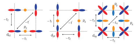
Figure 1: Schematic pictures of the hopping processes of the $t_{2g}$ orbitals on a two-dimensional layer. The difference in the color of each orbital shows the difference in the sign of its wave function.

First, $\hat{H}_{0}$ is given by

$$\hat{H}_{0} =\sum\limits_{\bm{k}}\sum\limits_{a,b=1}^{3}\sum\limits_{s=\uparrow,\downarrow}\epsilon_{ab}(\bm{k})\hat{c}^{\dagger}_{\bm{k}as}\hat{c}_{\bm{k}bs}.$$ (2)

Here $\hat{c}_{\bm{k}as}$ and $\hat{c}^{\dagger}_{\bm{k}as}$ are the annihilation and the creation operator of an electron of momentum $\bm{k}$, orbital $a$, and spin $s$, and $\epsilon_{ab}(\bm{k})$ is given by

$$\epsilon_{11}(\bm{k})= -\frac{\Delta_{t_{2g}}}{3}-2t_{1}\cos k_{x}-2t_{2}\cos k_{y}-\mu,$$ (3)

$$\epsilon_{12}(\bm{k})= \ \epsilon_{21}(\bm{k})=\ 4t^{\prime}\sin k_{x}\sin k_{y},$$ (4)

$$\epsilon_{22}(\bm{k})= -\frac{\Delta_{t_{2g}}}{3}-2t_{2}\cos k_{x}-2t_{1}\cos k_{y}-\mu,$$ (5)

$$\epsilon_{33}(\bm{k})= \ \frac{2\Delta_{t_{2g}}}{3}-2t_{3}(\cos k_{x}+\cos k_{y})$$

$$-4t_{4}\cos k_{x}\cos k_{y}-\mu,$$ (6)

and otherwise $\epsilon_{ab}(\bm{k})=0$, where $\Delta_{t_{2g}}$ is the difference between the crystalline-electric-field energies of the $d_{xy}$ and the $d_{xz/yz}$ orbital, $\mu$ is the chemical potential determined so that the electron number per site, $n_{\textrm{e}}$, satisfies $n_{\textrm{e}}=4$, and $t_{1}$, $t_{2}$, $t_{3}$, $t_{4}$, and $t^{\prime}$ are the hopping integrals of the $t_{2g}$ orbitals, whose schematic pictures are shown in Fig. 1. Since I neglect the effects Terakura ; NA-GA of the RuO₆ distortions on $\hat{H}_{0}$, the targets of this paper are the $214$-type ruthenates without the RuO₆ distortions.

Assuming that the LDA Oguchi ; Mazin-LDA for Sr₂RuO₄ gives a good starting point to include many-body effects in the $214$-type ruthenates without the RuO₆ distortions, I choose the parameters in $\epsilon_{ab}(\bm{k})$ so as to reproduce the electronic structure obtained in the LDA Oguchi ; Mazin-LDA for Sr₂RuO₄. Namely, I set $t_{1}=0.675$ eV, $t_{2}=0.09$ eV, $t_{3}=0.45$ eV, $t_{4}=0.18$ eV, $t^{\prime}=0.03$ eV, and $\Delta_{t_{2g}}=0.13$ eV. As explained in Ref. NA-review, , the obtained electronic structure is consistent with the LDA Oguchi ; Mazin-LDA : the bandwidth for the $t_{2g}$ orbitals is about $4$ eV; the quasi-one-dimensional $d_{xz}$ and $d_{yz}$ orbitals form the hole-like $\alpha$ and electron-like $\beta$ sheets, and the quasi-two-dimensional $d_{xy}$ orbital forms the electron-like $\gamma$ sheet; the van Hove singularity of the $d_{xy}$ orbital exists above the Fermi level; the occupation numbers of the $d_{xz/yz}$ and the $d_{xy}$ orbital are $n_{xz/yz}=1.38$ and $n_{xy}=1.25$.

Then, $\hat{H}_{\textrm{int}}$ is given by

$$\hat{H}_{\textrm{int}}= \dfrac{1}{4}\sum\limits_{\bm{j}}\sum\limits_{\{a\}}\sum\limits_{\{s_{1}\}}U_{abcd}^{s_{1}s_{2}s_{3}s_{4}}\hat{c}^{\dagger}_{\bm{j}as_{1}}\hat{c}^{\dagger}_{\bm{j}ds_{4}}\hat{c}_{\bm{j}cs_{3}}\hat{c}_{\bm{j}bs_{2}}$$

$$= \ U\sum\limits_{\bm{j}}\sum\limits_{a=1}^{3}\hat{n}_{\bm{j}a\uparrow}\hat{n}_{\bm{j}a\downarrow}+U^{\prime}\sum\limits_{\bm{j}}\sum\limits_{a=1}^{3}\sum\limits_{b<a}\hat{n}_{\bm{j}a}\hat{n}_{\bm{j}b}$$

$$-J_{\textrm{H}}\sum\limits_{\bm{j}}\sum\limits_{a=1}^{3}\sum\limits_{b<a}(2\hat{\bm{s}}_{\bm{j}a}\cdot\hat{\bm{s}}_{\bm{j}b}+\frac{1}{2}\hat{n}_{\bm{j}a}\hat{n}_{\bm{j}b})$$

$$+J^{\prime}\sum\limits_{\bm{j}}\sum\limits_{a=1}^{3}\sum\limits_{b\neq a}\hat{c}_{\bm{j}a\uparrow}^{\dagger}\hat{c}_{\bm{j}a\downarrow}^{\dagger}\hat{c}_{\bm{j}b\downarrow}\hat{c}_{\bm{j}b\uparrow}.$$ (7)

Here $U_{abcd}^{s_{1}s_{2}s_{3}s_{4}}$ is a bare four-point vertex function, $U$ is intraobital Coulomb interaction, $U^{\prime}$ is interorbital Coulomb interaction, $J_{\textrm{H}}$ is Hund’s rule coupling, $J^{\prime}$ is pair hopping term, $\hat{n}_{\bm{j}a}$ is $\hat{n}_{\bm{j}a}=\sum_{s}\hat{n}_{\bm{j}as}=\sum_{s}\hat{c}^{\dagger}_{\bm{j}as}\hat{c}_{\bm{j}as}$, and $\hat{\bm{s}}_{\bm{j}a}$ is $\hat{\bm{s}}_{\bm{j}a}=\frac{1}{2}\sum_{s,s^{\prime}}\hat{c}^{\dagger}_{\bm{j}as}\bm{\sigma}_{ss^{\prime}}\hat{c}_{\bm{j}as^{\prime}}$ with the Pauli matrices $\bm{\sigma}_{ss^{\prime}}$. Among the terms of $U_{abcd}^{s_{1}s_{2}s_{3}s_{4}}$, it is sufficient for a PM state to use $U_{abcd}^{\uparrow\downarrow}$, $U_{abcd}^{\uparrow\uparrow}$, and $U_{abcd}^{\pm}$, which are, respectively, $U^{\uparrow\downarrow}_{abcd}\equiv U_{abcd}^{\uparrow\uparrow\downarrow\downarrow}=U_{abcd}^{\downarrow\downarrow\uparrow\uparrow}$, $U^{\uparrow\uparrow}_{abcd}\equiv U_{abcd}^{\uparrow\uparrow\uparrow\uparrow}=U_{abcd}^{\downarrow\downarrow\downarrow\downarrow}$, and $U^{\pm}_{abcd}\equiv U_{abcd}^{\uparrow\downarrow\uparrow\downarrow}=U_{abcd}^{\downarrow\uparrow\downarrow\uparrow}$. In addition, in the absence of the spin-orbit interaction, it is more useful to introduce bare four-point vertex functions in spin and charge sector, $U_{abcd}^{\textrm{C}}$ and $U_{abcd}^{\textrm{S}}$, defined as

$$U_{abcd}^{s_{1}s_{2}s_{3}s_{4}}=\frac{1}{2}U_{abcd}^{\textrm{C}}\sigma_{s_{1}s_{2}}^{0}\sigma_{s_{4}s_{3}}^{0}-\frac{1}{2}U_{abcd}^{\textrm{S}}\bm{\sigma}_{s_{1}s_{2}}\cdot\bm{\sigma}_{s_{4}s_{3}}.$$ (8)

Namely, $U_{abcd}^{\textrm{C}}$ is $U_{abcd}^{\textrm{C}}=U^{\uparrow\downarrow}_{abcd}+U^{\uparrow\uparrow}_{abcd}$, and $U_{abcd}^{\textrm{S}}$ is $U_{abcd}^{\textrm{S}}=U^{\uparrow\downarrow}_{abcd}-U^{\uparrow\uparrow}_{abcd}=-U^{\pm}_{abcd}$.

I will explain how to treat the effects of $\hat{H}_{\textrm{int}}$ in Sec. II C, and how to choose the values of $U$, $U^{\prime}$, $J_{\textrm{H}}$, and $J^{\prime}$ in Sec. III.

In the effective model, I neglect the spin-orbit interaction of the Ru $t_{2g}$ orbitals for simplicity. This treatment may be sufficient to discuss the electronic properties analyzed in this paper since the coupling constant estimated in local-spin-density approximation Oguchi-LS for Sr₂RuO₄ is $0.167$ eV, which is smaller than the main terms of $\hat{H}_{0}$ and $\hat{H}_{\textrm{int}}$, and since its effects will not qualitatively change the results shown in Sect. III. (The main terms of $\hat{H}_{\textrm{int}}$ are of the order of magnitude $1$ eV, as described in Sec. III.) For several expected roles of the spin-orbit interaction, see the remaining issues in Sec. V.

II.2 Extended Éliashberg theory to charge transports of a multiorbital system

In this section, we derive the dc longitudinal conductivity without an external magnetic field and the dc transverse conductivity in a weak-field limit in the linear-response theory with the most-divergent-term approximation. In Sec. II B 1, we derive the dc longitudinal conductivity to analyze the resistivity of a correlated multiorbital system. After deriving the exact expression in terms of the four-point vertex function or the three-point vector vertex function, we derive its approximate expression in the most-divergent-term approximation Eliashberg-theory , which is appropriate for the metallic systems with long-lived QPs at (at least) several momenta. We also explain four general properties seen from the derived expression of the conductivity and show the properties of the resistivity about the dominant excitations, the dependence on the QP lifetime, and the main effects of the CVCs. In Sec. II B 2, to analyze the Hall coefficient of a correlated multiorbital system for a weak magnetic field, we derive the dc transverse conductivity in the weak-field limit. Due to difficulty deriving the exact expression, I derive only the approximate expression in the most-divergent-term approximation Fukuyama-RH ; Kohno-Yamada . In addition, after explaining four general properties of the derived conductivity, we deduce the properties of the Hall coefficient in the weak-field limit about the similar things for the resistivity.

Before the formal derivations, I remark on the meanings of taking the $\omega$ limit and holding $\omega\tau_{\textrm{trans}}\ll 1$ in these derivations NA-review with $\tau_{\textrm{trans}}$, the transport relaxation time Eliashberg-theory ; Fukuyama-RH (of the order of magnitude the QP damping). First, the $\omega$ limit, i.e. $\textstyle\lim_{\omega\rightarrow 0}\textstyle\lim_{\bm{q}\rightarrow\bm{0}}$, is vital to obtain the observable currents since the dynamic and uniform field causes the observable currents; on the other hand, the $\bm{q}$ limit, i.e. $\textstyle\lim_{\bm{q}\rightarrow\bm{0}}\textstyle\lim_{\omega\rightarrow 0}$, does not cause any observable currents as a result of the screening induced by the modulations of the charge distribution Yamada-text . Then, in taking $\textstyle\lim_{\omega\rightarrow 0}$, the QP lifetime should hold $\omega\tau_{\textrm{trans}}\ll 1$ since the inequality characterizes the relaxation process of transports; in $\omega\tau_{\textrm{trans}}\ll 1$, local equilibrium is realized due to the rapid relaxation compared with $\omega^{-1}$, a typical time scale of the field, and then the QPs near the Fermi level mainly govern the electronic transports.

II.2.1 Resistivity

For discussions about the resistivity of a correlated multiorbital system, I use the Kubo formula Kubo-formula for the longitudinal conductivity, $\sigma_{\nu\nu}$, in the $\omega$ limit and $\omega\tau_{\textrm{trans}}\ll 1$,

$$\sigma_{\nu\nu}= \ 2\lim\limits_{\omega\rightarrow 0}\lim\limits_{\bm{q}\rightarrow\bm{0}}\dfrac{\tilde{K}_{\nu\nu}^{(\textrm{R})}(\bm{q},\omega)-\tilde{K}_{\nu\nu}^{(\textrm{R})}(\bm{q},0)}{i\omega}$$

$$= \ 2\lim\limits_{\omega\rightarrow 0}\dfrac{\tilde{K}_{\nu\nu}^{(\textrm{R})}(\bm{0},\omega)-\tilde{K}_{\nu\nu}^{(\textrm{R})}(\bm{0},0)}{i\omega},$$ (9)

where $\tilde{K}_{\nu\nu}^{(\textrm{R})}(\bm{0},\omega)$ is determined by $\tilde{K}_{\nu\nu}^{(\textrm{R})}(\bm{0},\omega)=\tilde{K}_{\nu\nu}(i\Omega_{n}\rightarrow\omega+i0+)$ with $\tilde{K}_{\nu\nu}(i\Omega_{n})$, being

$$\tilde{K}_{\nu\nu}(i\Omega_{n})$$

$$= \ \lim\limits_{\bm{q}\rightarrow\bm{0}}\dfrac{1}{N}\int^{T^{-1}}_{0}d\tau e^{i\Omega_{n}\tau}\langle\textrm{T}_{\tau}\hat{J}_{\bm{q}\nu}(\tau)\hat{J}_{-\bm{q}\nu}(0)\rangle$$

$$= \ \frac{1}{N}\sum\limits_{\bm{k},\bm{k}^{\prime}}\sum\limits_{\{a\}}\int^{T^{-1}}_{0}d\tau e^{i\Omega_{n}\tau}(v_{\bm{k}\nu})_{ba}(v_{\bm{k}^{\prime}\nu})_{cd}$$

$$\times\langle\textrm{T}_{\tau}\hat{c}_{\bm{k}b}^{\dagger}(\tau)\hat{c}_{\bm{k}a}(\tau)\hat{c}_{\bm{k}^{\prime}c}^{\dagger}\hat{c}_{\bm{k}^{\prime}d}\rangle$$

$$= -\frac{T}{N}\sum\limits_{\bm{k}}\sum\limits_{m}\sum\limits_{\{a\}}(v_{\bm{k}\nu})_{ba}(v_{\bm{k}\nu})_{cd}G_{ac}(\bm{k},i\epsilon_{m+n})G_{db}(\bm{k},i\epsilon_{m})$$

$$-\frac{T^{2}}{N^{2}}\sum\limits_{\bm{k},\bm{k}^{\prime}}\sum\limits_{m,m^{\prime}}\sum\limits_{\{a\}}\sum\limits_{\{A\}}(v_{\bm{k}\nu})_{ba}(v_{\bm{k}^{\prime}\nu})_{cd}G_{aA}(\bm{k},i\epsilon_{m+n})$$

$$\times G_{dD}(\bm{k}^{\prime},i\epsilon_{m^{\prime}})G_{Bb}(\bm{k},i\epsilon_{m})G_{Cc}(\bm{k}^{\prime},i\epsilon_{m^{\prime}+n})$$

$$\times\Gamma_{\{A\}}(\bm{k},i\epsilon_{m},\bm{k}^{\prime},i\epsilon_{m^{\prime}};\bm{0},i\Omega_{n}).$$ (10)

In Eq. (10), $(v_{\bm{k}\nu})_{ab}$ is the group velocity,

$$(v_{\bm{k}\nu})_{ab}=\frac{\partial\epsilon_{ab}(\bm{k})}{\partial k_{\nu}},$$ (11)

and $\Gamma_{\{A\}}(\bm{k},i\epsilon_{m},\bm{k}^{\prime},i\epsilon_{m^{\prime}};\bm{0},i\Omega_{n})$ is the reducible four-point vertex function, which is connected with the irreducible one through the Bethe-Salpeter equation Nozieres ,

$$\Gamma_{\{A\}}(\bm{k},i\epsilon_{m},\bm{k}^{\prime},i\epsilon_{m^{\prime}};\bm{0},i\Omega_{n})$$

$$= \ \Gamma_{\{A\}}^{(1)}(\bm{k},i\epsilon_{m},\bm{k}^{\prime},i\epsilon_{m^{\prime}};\bm{0},i\Omega_{n})$$

$$+\frac{T}{N}\sum\limits_{\bm{k}^{\prime\prime}}\sum\limits_{m^{\prime\prime}}\sum\limits_{\{A^{\prime}\}}\Gamma_{ABC^{\prime}D^{\prime}}(\bm{k},i\epsilon_{m},\bm{k}^{\prime\prime},i\epsilon_{m^{\prime\prime}};\bm{0},i\Omega_{n})$$

$$\ \ \times G_{C^{\prime}A^{\prime}}(\bm{k}^{\prime\prime},i\epsilon_{m^{\prime\prime}+n})G_{B^{\prime}D^{\prime}}(\bm{k}^{\prime\prime},i\epsilon_{m^{\prime\prime}})$$

$$\ \ \times\Gamma_{A^{\prime}B^{\prime}CD}^{(1)}(\bm{k}^{\prime\prime},i\epsilon_{m^{\prime\prime}},\bm{k}^{\prime},i\epsilon_{m^{\prime}};\bm{0},i\Omega_{n}).$$ (12)

The irreducible four-point vertex function can be determined in the way explained in Sec. II C.

To obtain an exact expression of $\sigma_{\nu\nu}$, we carry out the analytic continuations AGD ; Eliashberg-theory of the first and second terms of Eq. (10) by using the analytic properties of the single-particle Green’s function and the four-point vertex function. As we will carry out those analytic continuations in Appendix A, we obtain

$$\tilde{K}_{\nu\nu}^{(\textrm{R})}(\bm{0},\omega) =-\frac{1}{N}\sum\limits_{\bm{k},\bm{k}^{\prime}}\sum\limits_{\{a\}}(v_{\bm{k}\nu})_{ba}(v_{\bm{k}^{\prime}\nu})_{cd}\int^{\infty}_{-\infty}\dfrac{d\epsilon}{4\pi i}$$

$$\times\Bigl{[}\tanh\dfrac{\epsilon}{2T}K_{1;\{a\}}^{(\textrm{R})}(\bm{k},\bm{k}^{\prime};\epsilon;\omega)$$

$$\ \ +\Bigl{(}\tanh\dfrac{\epsilon+\omega}{2T}-\tanh\dfrac{\epsilon}{2T}\Bigr{)}K_{2;\{a\}}^{(\textrm{R})}(\bm{k},\bm{k}^{\prime};\epsilon;\omega)$$

$$\ \ -\tanh\dfrac{\epsilon+\omega}{2T}K_{3;\{a\}}^{(\textrm{R})}(\bm{k},\bm{k}^{\prime};\epsilon;\omega)\Bigr{]},$$ (13)

with $K_{l;\{a\}}^{(\textrm{R})}(\bm{k},\bm{k}^{\prime};\epsilon;\omega)$, being

$$K_{l;\{a\}}^{(\textrm{R})}(\bm{k},\bm{k}^{\prime};\epsilon;\omega) =\ g_{l;acdb}(k;\omega)\delta_{\bm{k},\bm{k}^{\prime}}$$

$$+\frac{1}{N}\int^{\infty}_{-\infty}\frac{d\epsilon^{\prime}}{4\pi i}\sum\limits_{\{A\}}\sum\limits_{l^{\prime}=1}^{3}g_{l;aABb}(k;\omega)$$

$$\ \ \ \times\mathcal{J}_{ll^{\prime};\{A\}}(k,k^{\prime};\omega)g_{l^{\prime};CcdD}(k^{\prime};\omega).$$ (14)

Here $\mathcal{J}_{ll^{\prime};\{A\}}(k,k^{\prime};\omega)$ is connected with the reducible four-point vertex function in real-frequency representation and is determined by the Bethe-Salpeter equation,

$$\mathcal{J}_{ll^{\prime};\{A\}}(k,k^{\prime};\omega)=\mathcal{J}^{(1)}_{ll^{\prime};\{A\}}(k,k^{\prime};\omega)$$

$$\ \ \ \ \ +\sum\limits_{l^{\prime\prime}=1}^{3}\dfrac{1}{N}\sum\limits_{\bm{k}^{\prime\prime}}\sum\limits_{\{A^{\prime}\}}\int^{\infty}_{-\infty}\frac{d\epsilon^{\prime\prime}}{4\pi i}\mathcal{J}_{ll^{\prime\prime};ABC^{\prime}D^{\prime}}(k,k^{\prime\prime};\omega)$$

$$\ \ \ \ \ \ \ \times g_{l^{\prime\prime};C^{\prime}A^{\prime}B^{\prime}D^{\prime}}(k^{\prime\prime};\omega)\mathcal{J}^{(1)}_{l^{\prime\prime}l^{\prime};A^{\prime}B^{\prime}CD}(k^{\prime\prime},k^{\prime};\omega),$$ (15)

with the similar connection between $\mathcal{J}^{(1)}_{ll^{\prime};\{A\}}(k,k^{\prime};\omega)$ and the irreducible four-point vertex function in real-frequency representation.

We also rewrite $\tilde{K}_{\nu\nu}^{(\textrm{R})}(\bm{0},\omega)$ in a more compact form by using the three-point vertex function in real-frequency representation, $\Lambda_{\nu;l;ab}(k;\omega)\equiv\Lambda_{\nu;l;ab}(\bm{k},\epsilon+\omega,\bm{k},\epsilon)$ (for the detail see Appendix B):

$$\tilde{K}_{\nu\nu}^{(\textrm{R})}(\bm{0},\omega)$$

$$= -\frac{1}{N}\sum\limits_{\bm{k}}\sum\limits_{\{a\}}(v_{\bm{k}\nu})_{ba}\int^{\infty}_{-\infty}\frac{d\epsilon}{4\pi i}$$

$$\times\Bigl{[}\tanh\frac{\epsilon}{2T}g_{1;acdb}(k;\omega)\Lambda_{\nu;1;cd}(k;\omega)$$

$$\ \ \ +\Bigl{(}\tanh\frac{\epsilon+\omega}{2T}-\tanh\frac{\epsilon}{2T}\Bigr{)}g_{2;acdb}(k;\omega)\Lambda_{\nu;2;cd}(k;\omega)$$

$$\ \ \ -\tanh\frac{\epsilon+\omega}{2T}g_{3;acdb}(k;\omega)\Lambda_{\nu;3;cd}(k;\omega)\Bigr{]}.$$ (16)

Because of the difficulty solving the exact expression of $\sigma_{\nu\nu}$, we use the most-divergent-term approximation, introduced by Éliashberg Eliashberg-theory , in order to derive an approximate expression. In this approximation Eliashberg-theory , we consider only the most divergent terms with respect to the QP lifetime in $\gamma_{\alpha}^{\ast}(\bm{k}_{\textrm{F}})/T\rightarrow 0$ with $\gamma_{\alpha}^{\ast}(\bm{k}_{\textrm{F}})$, the QP damping for band $\alpha$ at Fermi momentum $\bm{k}_{\textrm{F}}$. This approximation is based on the limiting properties AGD ; Nozieres of the pairs of two single-particle Green’s functions with external momentum and frequency, $\bm{q}$ and $\omega$, in $q\rightarrow 0$ and $\gamma_{\alpha}^{\ast}(\bm{k}_{\textrm{F}})/T\rightarrow 0$. More precisely, utilizing the limiting properties, we can use the approximation that among the pairs of two single-particle Green’s functions, only a retarded-advanced pair gives the leading dependence on the QP damping and the external momentum and frequency. Namely, we can approximate the leading dependence of $g_{1;acdb}(k;\omega)$, $g_{2;acdb}(k;\omega)$, and $g_{3;acdb}(k;\omega)$ to NA-review

$$g_{1;acdb}(k;\omega)\sim \sum\limits_{\alpha,\beta}(U_{\bm{k}})_{a\alpha}(U_{\bm{k}}^{\dagger})_{\alpha c}(U_{\bm{k}})_{d\beta}(U_{\bm{k}}^{\dagger})_{\beta b}$$

$$\times\dfrac{z_{\alpha}(\bm{k})z_{\beta}(\bm{k})}{[\epsilon-\xi_{\alpha}^{\ast}(\bm{k})+i0+][\epsilon-\xi_{\beta}^{\ast}(\bm{k})+i0+]},$$ (17)

$$g_{2;acdb}(k;\omega)\sim \ 2\pi i\sum\limits_{\alpha,\beta}(U_{\bm{k}})_{a\alpha}(U_{\bm{k}}^{\dagger})_{\alpha c}(U_{\bm{k}})_{d\beta}(U_{\bm{k}}^{\dagger})_{\beta b}$$

$$\times\dfrac{z_{\alpha}(\bm{k})z_{\beta}(\bm{k})\delta(\epsilon-\xi_{\alpha}^{\ast}(\bm{k}))}{\omega-\xi_{\alpha}^{\ast}(\bm{k})+\xi_{\beta}^{\ast}(\bm{k})+i[\gamma_{\alpha}^{\ast}(\bm{k})+\gamma_{\beta}^{\ast}(\bm{k})]},$$ (18)

and

$$g_{3;acdb}(k;\omega)\sim \sum\limits_{\alpha,\beta}(U_{\bm{k}})_{a\alpha}(U_{\bm{k}}^{\dagger})_{\alpha c}(U_{\bm{k}})_{d\beta}(U_{\bm{k}}^{\dagger})_{\beta b}$$

$$\times\dfrac{z_{\alpha}(\bm{k})z_{\beta}(\bm{k})}{[\epsilon-\xi_{\alpha}^{\ast}(\bm{k})-i0+][\epsilon-\xi_{\beta}^{\ast}(\bm{k})-i0+]},$$ (19)

respectively. Here $\xi_{\alpha}^{\ast}(\bm{k})$ is the QP energy, $z_{\alpha}(\bm{k})$ is the mass enhancement factor, and $(U_{\bm{k}})_{a\alpha}$ is the unitary matrix to obtain the QP dispersions. Since this treatment remains reasonable for $\gamma_{\alpha}^{\ast}(\bm{k}_{\textrm{F}})/T<1$, the most-divergent-term approximation is not only exact in the FL but also appropriate in the correlated metallic systems having the long-lived QPs at least for several momenta.

To derive an approximate expression of $\sigma_{\nu\nu}$ in the most-divergent-term approximation Eliashberg-theory , we introduce two quantities, $\mathcal{J}^{(0)}_{ll^{\prime};\{a\}}(k,k^{\prime};\omega)$ and $\Lambda_{\nu;l;ab}^{(0)}(k;\omega)$, which are irreducible only about a retarded-advanced pair, and rewrite $\tilde{K}_{\nu\nu}^{(\textrm{R})}(\bm{0},\omega)$ by using the two quantities. First, we define $\mathcal{J}^{(0)}_{ll^{\prime};\{a\}}(k,k^{\prime};\omega)$ and $\Lambda_{\nu;l;ab}^{(0)}(k;\omega)$ as

$$\mathcal{J}^{(0)}_{ll^{\prime};\{a\}}(k,k^{\prime};\omega)=\mathcal{J}^{(1)}_{ll^{\prime};\{a\}}(k,k^{\prime};\omega)$$

$$\ \ \ \ \ +\dfrac{1}{N}\sum\limits_{\bm{k}^{\prime\prime}}\sum\limits_{\{A\}}\int^{\infty}_{-\infty}\frac{d\epsilon^{\prime\prime}}{4\pi i}\sum\limits_{l^{\prime\prime}=1,3}\mathcal{J}^{(0)}_{ll^{\prime\prime};abCD}(k,k^{\prime\prime};\omega)$$

$$\ \ \ \ \ \ \ \times g_{l^{\prime\prime};CABD}(k^{\prime\prime};\omega)\mathcal{J}^{(1)}_{l^{\prime\prime}l^{\prime};ABcd}(k^{\prime\prime},k^{\prime};\omega),$$ (20)

and

$$\Lambda_{\nu;l;ab}^{(0)}(k;\omega)=(v_{\bm{k}\nu})_{ab}$$

$$\ \ \ \ +\sum\limits_{\{A\}}\sum\limits_{l^{\prime}=1,3}\dfrac{1}{N}\sum\limits_{\bm{k}^{\prime}}\int^{\infty}_{-\infty}\frac{d\epsilon^{\prime}}{4\pi i}\mathcal{J}^{(0)}_{ll^{\prime};abCD}(k,k^{\prime};\omega)$$

$$\ \ \ \ \times g_{l^{\prime};CABD}(k^{\prime};\omega)(v_{\bm{k}^{\prime}\nu})_{AB},$$ (21)

respectively. We can also connect $\Lambda_{\nu;l;ab}^{(0)}(k;\omega)$ with $\Lambda_{\nu;l;ab}(k;\omega)$ as follows:

$$\Lambda_{\nu;l;ab}(k;\omega)=\Lambda_{\nu;l;ab}^{(0)}(k;\omega)$$

$$\ \ \ \ +\sum\limits_{\{A\}}\dfrac{1}{N}\sum\limits_{\bm{k}^{\prime}}\int^{\infty}_{-\infty}\dfrac{d\epsilon^{\prime}}{4\pi i}\mathcal{J}^{(0)}_{l2;abCD}(k,k^{\prime};\omega)$$

$$\ \ \ \ \times g_{2;CABD}(k^{\prime};\omega)\Lambda_{\nu;2;AB}(k^{\prime};\omega).$$ (22)

Then, substituting Eq. (22) into Eq. (16) and using two equalities,

$$-\frac{1}{N}\sum\limits_{\bm{k}}\sum\limits_{\{a\}}\int^{\infty}_{-\infty}\frac{d\epsilon}{4\pi i}(v_{\bm{k}\nu})_{ba}\tanh\frac{\epsilon}{2T}g_{1;acdb}(k;\omega)$$

$$\times\frac{1}{N}\sum\limits_{\bm{k}^{\prime}}\sum\limits_{\{A\}}\int^{\infty}_{-\infty}\frac{d\epsilon^{\prime}}{4\pi i}\mathcal{J}_{12;cdCD}^{(0)}(k,k^{\prime};\omega)g_{2;CABD}(k^{\prime};\omega)$$

$$\times\Lambda_{\nu;2;AB}(k^{\prime};\omega)$$

$$= -\frac{1}{N}\sum\limits_{\bm{k}}\sum\limits_{\{a\}}\int^{\infty}_{-\infty}\frac{d\epsilon}{4\pi i}\Bigl{[}\frac{1}{N}\sum\limits_{\bm{k}^{\prime}}\sum\limits_{\{A\}}\int^{\infty}_{-\infty}\frac{d\epsilon^{\prime}}{4\pi i}$$

$$\times\mathcal{J}_{21;baBA}^{(0)}(\bm{k},\epsilon,\bm{k},\epsilon+\omega,\bm{k}^{\prime},\epsilon^{\prime},\bm{k}^{\prime},\epsilon^{\prime}+\omega)$$

$$\times g_{1;BDCA}(\bm{k}^{\prime},\epsilon^{\prime},\bm{k}^{\prime},\epsilon^{\prime}+\omega)(v_{\bm{k}^{\prime}\nu})_{DC}\Bigr{]}$$

$$\times\Bigl{(}\tanh\frac{\epsilon+\omega}{2T}-\tanh\frac{\epsilon}{2T}\Bigr{)}g_{2;acdb}(k;\omega)\Lambda_{\nu;2;cd}(k;\omega),$$ (23)

and

$$\frac{1}{N}\sum\limits_{\bm{k}}\sum\limits_{\{a\}}\int^{\infty}_{-\infty}\frac{d\epsilon}{4\pi i}(v_{\bm{k}\nu})_{ba}\tanh\frac{\epsilon+\omega}{2T}g_{3;acdb}(k;\omega)$$

$$\times\frac{1}{N}\sum\limits_{\bm{k}^{\prime}}\sum\limits_{\{A\}}\int^{\infty}_{-\infty}\frac{d\epsilon^{\prime}}{4\pi i}\mathcal{J}_{32;cdCD}^{(0)}(k,k^{\prime};\omega)g_{2;CABD}(k^{\prime};\omega)$$

$$\times\Lambda_{\nu;2;AB}(k^{\prime};\omega)$$

$$= -\frac{1}{N}\sum\limits_{\bm{k}}\sum\limits_{\{a\}}\int^{\infty}_{-\infty}\frac{d\epsilon}{4\pi i}\Bigl{[}\frac{1}{N}\sum\limits_{\bm{k}^{\prime}}\sum\limits_{\{A\}}\int^{\infty}_{-\infty}\frac{d\epsilon^{\prime}}{4\pi i}$$

$$\times\mathcal{J}_{23;baBA}^{(0)}(\bm{k},\epsilon,\bm{k},\epsilon+\omega,\bm{k}^{\prime},\epsilon^{\prime},\bm{k}^{\prime},\epsilon^{\prime}+\omega)$$

$$\times g_{3;BDCA}(\bm{k}^{\prime},\epsilon^{\prime},\bm{k}^{\prime},\epsilon^{\prime}+\omega)(v_{\bm{k}^{\prime}\nu})_{DC}\Bigr{]}$$

$$\times\Bigl{(}\tanh\frac{\epsilon+\omega}{2T}-\tanh\frac{\epsilon}{2T}\Bigr{)}g_{2;acdb}(k;\omega)\Lambda_{\nu;2;cd}(k;\omega),$$ (24)

we can express $\tilde{K}_{\nu\nu}^{(\textrm{R})}(\bm{0},\omega)$ as two parts, the part excluding a retarded-advanced pair and the other part:

$$\tilde{K}_{\nu\nu}^{(\textrm{R})}(\bm{0},\omega)= -\frac{1}{N}\sum\limits_{\bm{k}}\sum\limits_{\{a\}}(v_{\bm{k}\nu})_{ba}\int^{\infty}_{-\infty}\dfrac{d\epsilon}{4\pi i}$$

$$\times\Bigl{[}\tanh\dfrac{\epsilon}{2T}g_{1;acdb}(k;\omega)\Lambda_{\nu;1;cd}^{(0)}(k;\omega)$$

$$-\tanh\dfrac{\epsilon+\omega}{2T}g_{3;acdb}(k;\omega)\Lambda_{\nu;3;cd}^{(0)}(k;\omega)\Bigr{]}$$

$$-\frac{1}{N}\sum\limits_{\bm{k}}\sum\limits_{\{a\}}\int^{\infty}_{-\infty}\dfrac{d\epsilon}{4\pi i}\Lambda_{\nu;2;ba}^{(0)}(\bm{k},\epsilon,\bm{k},\epsilon+\omega)$$

$$\times\Bigl{(}\tanh\dfrac{\epsilon+\omega}{2T}-\tanh\dfrac{\epsilon}{2T}\Bigr{)}g_{2;acdb}(k;\omega)$$

$$\times\Lambda_{\nu;2;cd}(k;\omega).$$ (25)

This expression remains exact at this stage. In Eqs. (23) and (24), we have used Eqs. (86), (88), (90), and (92) and the exchange symmetry Kohno-Yamada of the four-point vertex function about its variables.

Adopting the most-divergent term approximation to Eq. (25), extracting the $\omega$-linear term, and using (9), we obtain an approximate expression of $\sigma_{\nu\nu}$,

$$\sigma_{\nu\nu}= \dfrac{2}{N}\sum\limits_{\bm{k}}\sum\limits_{\{a\}=1}^{3}\int^{\infty}_{-\infty}\dfrac{d\epsilon}{2\pi}\Bigl{(}-\dfrac{\partial f(\epsilon)}{\partial\epsilon}\Bigr{)}$$

$$\times\Lambda_{\nu;2;ba}^{(0)}(k;0)g_{2;acdb}(k;0)\Lambda_{\nu;2;cd}(k;0).$$ (26)

Here we can regard $\Lambda_{\nu;2;ba}^{(0)}(k;0)$ and $\Lambda_{\nu;2;cd}(k;0)$ as, respectively, the current including the CVC arising from the self-energy and the current including the CVCs arising from the self-energy and the irreducible four-point vertex function. This is because Eq. (21) for $l=2$ at $\omega=0$ becomes

$$\Lambda_{\nu;2;ab}^{(0)}(k;0)=(v_{\bm{k}\nu})_{ab}+\dfrac{\partial\textrm{Re}\Sigma_{ab}^{(\textrm{A})}(k)}{\partial k_{\nu}},$$ (27)

as a result of a Ward identity Nozieres , and because Eq. (22) for $l=2$ at $\omega=0$ becomes

$$\Lambda_{\nu;2;cd}(k;0)=\Lambda_{\nu;2;cd}^{(0)}(k;0)$$

$$\ \ \ \ +\frac{1}{N}\sum\limits_{\bm{k}^{\prime}}\sum\limits_{\{A\}}\int^{\infty}_{-\infty}\frac{d\epsilon^{\prime}}{4\pi i}\mathcal{J}_{22;cdCD}^{(1)}(k,k^{\prime};0)$$

$$\ \ \ \ \times g_{2;CABD}(k^{\prime};0)\Lambda_{\nu;2;AB}(k^{\prime};0),$$ (28)

as a result of the disappearance of the second term of Eq. (20), the higher-order term Eliashberg-theory about $\omega\tau_{\textrm{trans}}$ than the first term of Eq. (20). Note that the second term of Eq. (28) plays a similar role for the backflow correction Nozieres in the FL theory since that term connects the currents at $\bm{k}$ and $\bm{k}^{\prime}$.

From Eq. (26), we see four general properties for the dc longitudinal conductivity of a correlated electron system. (The following arguments for $\sigma_{xx}$ are qualitatively the same even for $\sigma_{yy}$.) First, due to the factor $(-\frac{\partial f(\epsilon)}{\partial\epsilon})$ in Eq. (26), the main excitations arise from the QPs near the Fermi level. This property indicates the importance of the coherent part of the single-particle Green’s function in discussing $\rho_{ab}$. Such importance holds even if its incoherent part evolves, as shown in dynamical-mean-field theory (DMFT) DMFT-trans-QP for a single-orbital Hubbard model on a square lattice in a PM metallic state near a Mott transition. Second, Eq. (26) with the approximate form of $g_{2;acdb}(k;0)$ shows that the intraband excitations become dominant compared with the interband excitations. This is because the intraband components of Eq. (18) (i.e., $\alpha=\beta$) give larger finite contributions to $\sigma_{xx}$ than the interband components (i.e., $\alpha\neq\beta$) due to the factor $-\xi_{\alpha}^{\ast}(\bm{k})+\xi_{\beta}^{\ast}(\bm{k})$ in the denominator of Eq. (18) for $\omega=0$. Third, combining Eqs. (26) and (18) with the above second general property, we find that $\sigma_{xx}$ is inversely proportional to the QP damping. Note that the dependence of $\sigma_{xx}$ on the QP damping can be determined by the dependence of $g_{2;acdb}(k;0)$ since $\Lambda_{x;2;ba}^{(0)}(k;0)$ and $\Lambda_{x;2;cd}(k;0)$ are independent of the QP damping Eliashberg-theory . Fourth, due to the CVCs in $\Lambda_{x;2;ba}^{(0)}(k;0)$ and $\Lambda_{x;2;cd}(k;0)$, $\sigma_{xx}$ is affected both by the CVC arising from the self-energy and by the CVCs arising from the self-energy and irreducible four-point vertex function, and the dominant effect arise from the magnitude changes of the currents. This property can be deduced from the following arguments: Since $\Lambda_{x;2;ba}^{(0)}(k;0)$ includes the $\Sigma$ CVC [see Eq. (27)], its effect is the renormalization of the group velocity, resulting in a magnitude change of the current Eliashberg-theory . On the other hand, the effects of the CVCs in $\Lambda_{x;2;cd}(k;0)$ are not only a magnitude change of the current but also an angle change since the CVC arising from the irreducible four-point vertex function connects the currents at $\bm{k}$ and $\bm{k}^{\prime}$, which are not always parallel or antiparallel Kon-CVC . Those effects on $\sigma_{xx}$ can be described by

$$\Lambda_{x;2;ba}^{(0)}(k;0)\Lambda_{x;2;cd}(k;0)$$

$$= |\Lambda_{2;ba}^{(0)}(k)|\cos\varphi_{ba}^{(0)}(k)|\Lambda_{2;cd}(k)|\cos\varphi_{cd}(k)$$

$$\sim |\Lambda_{2;ba}^{(0)}(k)|\cos\varphi_{ba}^{(0)}(k)|\Lambda_{2;cd}(k)|\cos\varphi_{cd}^{(0)}(k)[1-\tfrac{\Delta\varphi_{cd}(k)^{2}}{2}],$$ (29)

where $|\Lambda_{2;ab}^{(0)}(k)|$ and $|\Lambda_{2;ab}(k)|$ represent the magnitudes of $\Lambda_{x;2;ba}^{(0)}(k;0)$ and $\Lambda_{x;2;cd}(k;0)$, respectively, and $\varphi_{ab}^{(0)}(k)$ and $\varphi_{ab}(k)=\varphi_{ab}^{(0)}(k)+\Delta\varphi_{ab}(k)$ represent the angles. Thus, even for the CVCs in $\Lambda_{x;2;cd}(k;0)$, the magnitude change is dominant for $\sigma_{xx}$.

From those properties, we can deduce the properties of the resistivity about the dominant excitations, the dependence on the QP lifetime, and the main effects of the CVCs. Since the resistivity is the inverse of the longitudinal conductivity, the dominant excitations and the main effects of the CVCs are the same for $\sigma_{xx}$, and the resistivity is inversely proportional to the QP lifetime (in the same way for the relaxation-time approximation Ziman ).

II.2.2 Hall coefficient

For discussions of the usual Hall effect of a correlated multiorbital system for a weak external magnetic field, we consider a uniform static external magnetic field along the $z$-direction, which is so weak that the cyclotron frequency, $\omega_{\textrm{c}}$, satisfies $\omega_{\textrm{c}}\tau_{\textrm{trans}}\ll 1$, and derive an approximate expression of the Hall coefficient in the weak-field limit on the basis of the linear-response theory in the most-divergent-term approximation Fukuyama-RH ; Kohno-Yamada . In this derivation, we assume that the system has the mirror symmetries about the $xz$- and the $yz$-plane and the equivalence between the $x$- and the $y$-direction Kohno-Yamada ; these are valid for some 214-type ruthenates without the RuO₆ distortions. Because of the mirror symmetries and the Onsager reciprocal theorem Onsager-thm1 ; Onsager-thm2 , we can treat the Hall coefficient, which is generally a third-rank axial tensor Konno , as a scalar. In addition, because of the equivalence between the $x$- and the $y$-direction, the Hall coefficient in the linear-response theory Kubo-formula in the weak-field limit becomes

$$R_{\textrm{H}}= \dfrac{1}{\sigma_{xx}\sigma_{yy}}\lim\limits_{H\rightarrow 0}\dfrac{\sigma_{xy}}{H}$$

$$= \dfrac{1}{\sigma_{xx}^{2}}\lim\limits_{H\rightarrow 0}\dfrac{\sigma_{xy}}{H}.$$ (30)

Since we had derived $\sigma_{xx}$ in Sect. II B 1, we need to calculate $\lim\limits_{H\rightarrow 0}\frac{\sigma_{xy}}{H}$ in the linear-response theory with the most-divergent-term approximation Fukuyama-RH ; Kohno-Yamada in this section.

To calculate $\lim\limits_{H\rightarrow 0}\frac{\sigma_{xy}}{H}$, we need to derive the $H$-linear terms of $\sigma_{xy}$. For that purpose, we use the vector potential, $\bm{A}$, instead of $H$ itself, and derive the $\bm{q}$-linear and $\bm{A}$-linear terms. Thus, the Kubo formula for $\lim\limits_{H\rightarrow 0}\frac{\sigma_{xy}}{H}$ becomes Fukuyama-RH ; Kohno-Yamada

$$\lim\limits_{H\rightarrow 0}\dfrac{\sigma_{xy}}{H}= 2\lim\limits_{\omega\rightarrow 0}\lim\limits_{\bm{q}\rightarrow 0}\dfrac{1}{i(q_{x}A_{y}(\bm{q})-q_{y}A_{x}(\bm{q}))e^{i\bm{q}\cdot\bm{r}}}$$

$$\times\dfrac{\Phi_{xy}^{(\textrm{R})}(\bm{q},\omega)-\Phi_{xy}^{(\textrm{R})}(\bm{q},0)}{i\omega},$$ (31)

where $\Phi_{xy}^{(\textrm{R})}(\bm{q},\omega)$ is obtained by $\Phi_{xy}^{(\textrm{R})}(\bm{q},\omega)=\Phi_{xy}(\bm{q},i\Omega_{n}\rightarrow\omega+i0+)$ with

$$\Phi_{xy}(\bm{q},i\Omega_{n})= \dfrac{T}{N}\int^{T^{-1}}_{0}d\tau\int^{T^{-1}}_{0}d\tau^{\prime}e^{i\Omega_{n}(\tau-\tau^{\prime})}$$

$$\times\langle\textrm{T}_{\tau}\hat{J}_{x}^{H}(\bm{q},\tau)\hat{J}_{y}^{H}(\bm{0},\tau^{\prime})\rangle_{H}$$

$$= \sum\limits_{\nu}K_{xy\nu}(\bm{q},i\Omega_{n})A_{\nu}(\bm{q}).$$ (32)

Here $\hat{\bm{J}}^{\textrm{H}}(\bm{0})$ within the linear response becomes

$$\hat{\bm{J}}^{\textrm{H}}(\bm{0})-\hat{\bm{J}}(\bm{0})=-\sum\limits_{\bm{k}}\sum\limits_{a,b}\bm{A}(\bm{q})\cdot\bm{\nabla}_{\bm{k}}(\bm{v}_{\bm{k}})_{ba}\hat{c}^{\dagger}_{\bm{k}b}\hat{c}_{\bm{k}a},$$ (33)

and $K_{xy\nu}^{(\textrm{R})}(\bm{q},\omega)$ is obtained by $K_{xy\nu}^{(\textrm{R})}(\bm{q},\omega)=K_{xy\nu}(\bm{q},i\Omega_{n}\rightarrow\omega+i0+)$, where $K_{xy\nu}(\bm{q},i\Omega_{n})$ is given by

$$K_{xy\nu}(\bm{q},i\Omega_{n}) =-\delta_{\nu,y}\frac{T}{N}\int^{T^{-1}}_{0}d\tau\int^{T^{-1}}_{0}d\tau^{\prime}e^{i\Omega_{n}(\tau-\tau^{\prime})}$$

$$\times\langle\textrm{T}_{\tau}\hat{J}_{x}(\bm{q},\tau)\sum\limits_{\bm{k}}\sum\limits_{a,b}\frac{\partial(v_{\bm{k}y})_{ba}}{\partial k_{\nu}}\hat{c}^{\dagger}_{\bm{k}b}(\tau^{\prime})\hat{c}_{\bm{k}a}(\tau^{\prime})\rangle$$

$$+\frac{T}{N}\int^{T^{-1}}_{0}d\tau\int^{T^{-1}}_{0}d\tau^{\prime}\int^{T^{-1}}_{0}d\tau^{\prime\prime}e^{i\Omega_{n}(\tau-\tau^{\prime})}$$

$$\times\langle\textrm{T}_{\tau}\hat{J}_{x}(\bm{q},\tau)\hat{J}_{y}(\bm{0},\tau^{\prime})\hat{J}_{\nu}(-\bm{q},\tau^{\prime\prime})\rangle.$$ (34)

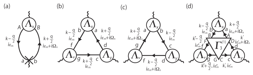
Figure 2: Diagrammatic representations of (a) the first, (b) the second, (c) the third, and (d) the fourth term of Eq. (35). $\times$ in panel (a) represents the momentum derivative.

Furthermore, using the three-point vector vertex function and introducing the irreducible six-point vertex function Fukuyama-RH ; Kohno-Yamada , we can rewrite Eq. (34) as

$$K_{xy\nu}(\bm{q},i\Omega_{n})= \ \delta_{\nu,y}\frac{T}{N}\sum\limits_{\bm{k}}\sum\limits_{m}\sum\limits_{a,b,A,B}\dfrac{\partial(v_{\bm{k}y})_{ba}}{\partial k_{\nu}}G_{aA}(\bm{k}_{-},i\epsilon_{m})\Lambda_{x;AB}(\bm{k}_{-},i\epsilon_{m},\bm{k}_{+},i\epsilon_{m+n})G_{Bb}(\bm{k}_{+},i\epsilon_{m+n})$$

$$+\frac{T}{N}\sum\limits_{\bm{k}}\sum\limits_{m}\sum\limits_{\{a\}}\sum\limits_{f,g}G_{fb}(\bm{k}_{-},i\epsilon_{m})\Lambda_{x;ba}(\bm{k}_{-},i\epsilon_{m},\bm{k}_{+},i\epsilon_{m+n})G_{ad}(\bm{k}_{+},i\epsilon_{m+n})$$

$$\ \ \times\Lambda_{\nu;gf}(\bm{k}_{+},i\epsilon_{m},\bm{k}_{-},i\epsilon_{m})G_{cg}(\bm{k}_{+},i\epsilon_{m})\Lambda_{y;dc}(\bm{k}_{+},i\epsilon_{m+n},\bm{k}_{+},i\epsilon_{m})$$

$$+\frac{T}{N}\sum\limits_{\bm{k}}\sum\limits_{m}\sum\limits_{\{a\}}\sum\limits_{f,g}G_{ag}(\bm{k}_{+},i\epsilon_{m+n})\Lambda_{x;ba}(\bm{k}_{-},i\epsilon_{m},\bm{k}_{+},i\epsilon_{m+n})G_{cb}(\bm{k}_{-},i\epsilon_{m})$$

$$\ \ \times\Lambda_{\nu;gf}(\bm{k}_{+},i\epsilon_{m+n},\bm{k}_{-},i\epsilon_{m+n})G_{fd}(\bm{k}_{-},i\epsilon_{m+n})\Lambda_{y;dc}(\bm{k}_{-},i\epsilon_{m+n},\bm{k}_{-},i\epsilon_{m})$$

$$+\Bigl{(}\frac{T}{N}\Bigr{)}^{3}\sum\limits_{\bm{k},\bm{k}^{\prime},\bm{k}^{\prime\prime}}\sum\limits_{m,m^{\prime},m^{\prime\prime}}\sum\limits_{\{a\}}\sum\limits_{\{A\}}\sum\limits_{f,g,F,G}G_{Bb}(\bm{k}_{-},i\epsilon_{m})\Lambda_{x;ba}(\bm{k}_{-},i\epsilon_{m},\bm{k}_{+},i\epsilon_{m+n})G_{aA}(\bm{k}_{+},i\epsilon_{m+n})$$

$$\ \ \times G_{Gg}(\bm{k}^{\prime\prime}_{+},i\epsilon_{m^{\prime\prime}})\Lambda_{\nu;gf}(\bm{k}^{\prime\prime}_{+},i\epsilon_{m^{\prime\prime}},\bm{k}^{\prime\prime}_{-},i\epsilon_{m^{\prime\prime}})G_{fF}(\bm{k}^{\prime\prime}_{-},i\epsilon_{m^{\prime\prime}})G_{Dd}(\bm{k}^{\prime},i\epsilon_{m^{\prime}+n})\Lambda_{y;dc}(\bm{k}^{\prime},i\epsilon_{m^{\prime}+n},\bm{k}^{\prime},i\epsilon_{m^{\prime}})$$

$$\ \ \times G_{cC}(\bm{k}^{\prime},i\epsilon_{m^{\prime}})\Gamma_{3;ABCDFG}^{(1)}(\bm{k}_{+},i\epsilon_{m+n},\bm{k}_{-},i\epsilon_{m};\bm{k}^{\prime},i\epsilon_{m^{\prime}},\bm{k}^{\prime},i\epsilon_{m^{\prime}+n};\bm{k}^{\prime\prime}_{-},i\epsilon_{m^{\prime\prime}},\bm{k}^{\prime\prime}_{+},i\epsilon_{m^{\prime\prime}}),$$ (35)

with $\bm{k}_{\pm}\equiv\bm{k}\pm\frac{\bm{q}}{2}$. The terms of Eq. (35) can be represented by the diagrams shown in Fig. 2. Thus, the remaining tasks are to derive the $\bm{q}$-linear terms of $K_{xy\nu}(\bm{q},i\Omega_{n})$, to carry out its analytic continuation, and to combine the result with Eqs. (31) and (32).

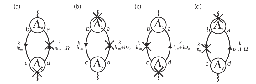
Figure 3: Diagrammatic representation of each term of Eq. (36). The minus signs of the diagrams in panels (b) and (c) are not explicitly written. $\times$ represents the momentum derivative.

We first derive the $\bm{q}$-linear terms of Eq. (35) in the most-divergent-term approximation Fukuyama-RH ; Kohno-Yamada . As I will explain in Appendix C in detail, the $\bm{q}$-linear terms are given by

$$K_{xy\nu}(\bm{q},i\Omega_{n})=\frac{1}{2}(q_{x}\delta_{\nu,y}-q_{y}\delta_{\nu,x})\frac{T}{N}\sum\limits_{\bm{k}}\sum\limits_{m}\sum\limits_{\{a\}}$$

$$\times\Bigl{[}\Lambda_{x;ba}(\bm{k},i\epsilon_{m},\bm{k},i\epsilon_{m+n})\dfrac{\overleftrightarrow{\partial}}{\partial k_{y}}\Lambda_{y;dc}(\bm{k},i\epsilon_{m+n},\bm{k},i\epsilon_{m})\Bigr{]}$$

$$\times\Bigl{[}G_{cb}(\bm{k},i\epsilon_{m})\dfrac{\overleftrightarrow{\partial}}{\partial k_{x}}G_{ad}(\bm{k},i\epsilon_{m+n})\Bigr{]}.$$ (36)

We can show the four terms of Eq. (36) as the diagrams in Fig. 3.

Then, we carry out the analytic continuation of Eq. (36). This procedure can be done in the same way for $\sigma_{\nu\nu}$ in Sect. II B 1 since the relevant parameter for analytic continuations about frequency is the frequency dependence and since the frequency dependence of Eq. (36) is the same as $\tilde{K}_{\nu\nu}(i\Omega_{n})$ expressed in terms of the three-point vector vertex function,

$$\tilde{K}_{\nu\nu}(i\Omega_{n})= -\frac{T}{N}\sum\limits_{\bm{k}}\sum\limits_{m}\sum\limits_{\{a\}}(v_{\bm{k}\nu})_{ba}\Lambda_{\nu;cd}(\bm{k},i\epsilon_{m};\bm{0},i\Omega_{n})$$

$$\times G_{ac}(\bm{k},i\epsilon_{m+n})G_{db}(\bm{k},i\epsilon_{m}).$$ (37)

Thus, we obtain $\Delta K_{xy\nu}^{(\textrm{R})}(\bm{q},\omega)\equiv K_{xy\nu}^{(\textrm{R})}(\bm{q},\omega)-K_{xy\nu}^{(\textrm{R})}(\bm{q},0)$ in the most-divergent-term approximation Fukuyama-RH ; Kohno-Yamada within the linear order of $\omega/T$:

$$\Delta K_{xy\nu}^{(\textrm{R})}(\bm{q},\omega)= -\frac{1}{2}(q_{x}\delta_{\nu,y}-q_{y}\delta_{\nu,x})\int^{\infty}_{-\infty}\frac{d\epsilon}{4\pi i}2\omega\Bigl{(}-\dfrac{\partial f(\epsilon)}{\partial\epsilon}\Bigr{)}$$

$$\times\frac{1}{N}\sum\limits_{\bm{k}}\sum\limits_{\{a\}}\Bigl{[}\Lambda_{x;2;ba}(k;0)\dfrac{\overleftrightarrow{\partial}}{\partial k_{y}}\Lambda_{y;2;dc}(k;0)\Bigr{]}$$

$$\times\Bigl{[}G_{ad}^{(\textrm{R})}(k)\dfrac{\overleftrightarrow{\partial}}{\partial k_{x}}G_{cb}^{(\textrm{A})}(k)\Bigr{]}.$$ (38)

As described in Sect. II B 1, in the most-divergent-term approximation Eliashberg-theory , the contribution from a retarded-retarded or an advanced-advanced pair of two single-particle Green’s functions is negligible compared with the contribution from a retarded-advanced pair.

Combining Eq. (38) with Eqs. (31) and (32), we finally obtain an approximate expression of the dc transverse conductivity in the weak-field limit within the most-divergent-term approximation:

$$\lim\limits_{H\rightarrow 0}\dfrac{\sigma_{xy}}{H}= \dfrac{1}{N}\sum\limits_{\bm{k}}\int^{\infty}_{-\infty}\frac{d\epsilon}{2\pi}\Bigl{(}-\dfrac{\partial f(\epsilon)}{\partial\epsilon}\Bigr{)}$$

$$\times\sum\limits_{\{a\}}\Bigl{[}\Lambda_{x;2;ba}(k;0)\dfrac{\overleftrightarrow{\partial}}{\partial k_{y}}\Lambda_{y;2;dc}(k;0)\Bigr{]}$$

$$\times\textrm{Im}\Bigl{[}G_{ad}^{(\textrm{R})}(k)\dfrac{\overleftrightarrow{\partial}}{\partial k_{x}}G_{cb}^{(\textrm{A})}(k)\Bigr{]}.$$ (39)

Adopting the similar arguments for $\sigma_{xx}$ in Sect. II B 1 to Eq. (39), we see four general properties for $\lim\limits_{H\rightarrow 0}\frac{\sigma_{xy}}{H}$. First, the QPs near the Fermi level are dominant due to the factor $(-\frac{\partial f(\epsilon)}{\partial\epsilon})$. This is the same for $\sigma_{xx}$. Second, the dominance of the intraband excitations also holds because of the similar reason for $\sigma_{xx}$. Note that we can obtain the finite intraband components in $\lim\limits_{H\rightarrow 0}\frac{\sigma_{xy}}{H}$ since the quantities in the former square bracket in Eq. (39) are odd about $k_{x}$ and even about $k_{y}$ due to the combination of the $k_{x}$ derivative in $\Lambda_{x;2;ba}(k;0)$, $\frac{\overleftrightarrow{\partial}}{\partial k_{y}}$, and the $k_{y}$ derivative in $\Lambda_{y;2;dc}(k;0)$, and since the quantities in the latter are odd about $k_{x}$ and even about $k_{y}$ due to the combination of $\frac{\overleftrightarrow{\partial}}{\partial k_{x}}$ and a product of the retarded and the advanced single-particle Green’s function. Third, in contrast to $\sigma_{xx}$, $\lim\limits_{H\rightarrow 0}\frac{\sigma_{xy}}{H}$ is inversely proportional to the square of the QP damping. This is because the momentum derivative in a retarded-advanced pair leads to an additional factor of the inverse of the QP damping Fukuyama-RH ; Kohno-Yamada . Fourth, the CVCs in $\Lambda_{x;2;ba}(k;0)$ and $\Lambda_{y;2;dc}(k;0)$ affect $\lim\limits_{H\rightarrow 0}\frac{\sigma_{xy}}{H}$, and the dominant effects are an angle change, which is different from the fourth property for $\sigma_{xx}$. This property arises from the dependence of the following quantity on the magnitude and angle changes of the currents:

$$\Bigl{[}\Lambda_{x;2;ba}(k;0)\dfrac{\overleftrightarrow{\partial}}{\partial k_{y}}\Lambda_{y;2;dc}(k;0)\Bigr{]}$$

$$= |\Lambda_{2;ba}(k)|\cos\varphi_{ba}(k)|\Lambda_{2;dc}(k)|\cos\varphi_{dc}(k)\dfrac{\partial\varphi_{dc}(k)}{\partial k_{y}}$$

$$+ |\Lambda_{2;ba}(k)|\sin\varphi_{ba}(k)\dfrac{\partial\varphi_{ba}(k)}{\partial k_{y}}|\Lambda_{2;dc}(k)|\sin\varphi_{dc}(k)$$

$$\sim |\Lambda_{2;ba}(k)|\cos\varphi_{ba}^{(0)}(k)|\Lambda_{2;dc}(k)|\cos\varphi_{dc}^{(0)}(k)\dfrac{\partial\varphi_{dc}(k)}{\partial k_{y}}$$

$$+ |\Lambda_{2;ba}(k)|\sin\varphi_{ba}^{(0)}(k)\dfrac{\partial\varphi_{ba}(k)}{\partial k_{y}}|\Lambda_{2;dc}(k)|\sin\varphi_{dc}^{(0)}(k).$$ (40)

Thus, due to the appearance of $\frac{\partial\varphi_{dc}(k)}{\partial k_{y}}$ or $\frac{\partial\varphi_{ba}(k)}{\partial k_{y}}$, the angle change of the current causes a more drastic effect on $\textstyle\lim_{H\rightarrow 0}\frac{\sigma_{xy}}{H}$ than $\sigma_{xx}$. Actually, the importance of such drastic effect has been obtained in a single-orbital Hubbard model on a square lattice Kon-CVC .

Combining those properties with the four properties for $\sigma_{xx}$, we can deduce the properties of $R_{\textrm{H}}$ about the dominant excitations, the dependence on the QP lifetime, and the main effects of the CVCs. First, the dominant excitations are the intraband excitations near the Fermi level. Second, the dependence of the numerator and denominator of $R_{\textrm{H}}$ on the QP lifetime cancels each other out in the absence of the band dependence of the QP lifetime, while the cancellation is not perfect in the presence of the band dependence. This is because $\textstyle\lim_{H\rightarrow 0}\frac{\sigma_{xy}}{H}$ or $\sigma_{xx}$ consists of the sum of the corresponding intraband components, each of which has the dependence of the QP lifetime for the band. Note that the non-perfect cancellation is the origin of the temperature dependence of $R_{\textrm{H}}$ of a multiorbital system in the Fermi liquid. Third, the main effects of the CVCs on $R_{\textrm{H}}$ are the magnitude change of the current due to $\Lambda_{x;2;ba}^{(0)}(k;0)$ in the denominator of $R_{\textrm{H}}$ and the angle change of the current due to $\Lambda_{x;2;ba}(k;0)$ or $\Lambda_{y;2;dc}(k;0)$ in the numerator since there is the nearly perfect cancellation between the magnitude changes due to $\Lambda_{x;2;ba}(k;0)$ and $\Lambda_{y;2;dc}(k;0)$ in the numerator and due to the square of $\Lambda_{x;2;cd}(k;0)$ in the denominator.

II.3 FLEX approximation with the $\Sigma$ CVC, the MT CVC, and the AL CVC

In this section, after explaining several advantages of the FLEX approximation with the CVCs arising from the self-energy and irreducible four-point vertex function, I formulate the FLEX approximation in Matsubara-frequency representation for a multiorbital Hubbard model in a PM state and derive the CVCs arising from the irreducible four-point vertex function in the FLEX approximation. In the latter derivation, we first derive the irreducible four-point vertex function in Matsubara-frequency representation; second, we convert it into a real-frequency representation by using the analytic continuation; third, we calculate part of the kernel of the CVCs arising from the irreducible four-point vertex function; fourth, we derive the Bethe-Salpeter equation for the current including the CVCs. Furthermore, I introduce a simplified Bethe-Salpeter equation by approximating the AL CVC to its main terms.

To describe the electronic properties near or away from a magnetic QCP, I use the FLEX approximation with the CVCs arising from the self-energy and irreducible four-point vertex function since its following three properties are the advantages in describing the electronic transports. One is that this approximation is one of the conserving approximations FLEX1 ; FLEX2 ; FLEX3 that automatically satisfies conservation laws Luttinger-Ward ; Baym-Kadanoff . This is powerful to describe transports since the treatment in keeping conservation laws is essential in transports FLEX3 . Another advantage is that this approximation can take account of the many-body effects due to the self-energy itself and the CVCs arising from the self-energy and the irreducible four-point vertex function Kon-review ; NA-review . In particular, this approximation can sufficiently treat the effects of spatial (i.e., momentum-dependent) correlation even near a magnetic QCP Kon-review ; NA-review ; Yanase-review . Due to this advantage, the FLEX approximation with the CVCs can analyze how those many-body effects influence the electronic properties beyond random-phase approximation (RPA), a mean-field-type approximation, and the relaxation-time approximation Ziman , where all the CVCs are neglected Kon-review , and improve several unrealistic results in the RPA; examples of the improvements are a reasonable value of $U$ for a magnetic transition and the Curie-Weiss-type temperature dependence of the spin susceptibility near an AF QCP Yanase-review ; NA-review . (As described in Sect. II B, the CVCs are vital to satisfy conservation laws Yamada-Yosida ; Kon-review ; NA-review .) The other advantage is that the FLEX approximation can sufficiently describe the coherent parts of the single-particle Green’s function for a moderately strong electron correlation FLEX3 ; Yanase-review ; Kon-review ; NA-review . Actually, the FLEX approximation for a single-orbital Hubbard model on a square lattice at $U$ being a half of the bandwidth is in satisfactory agreement with the quantum Monte Carlo calculation about the imaginary-time dependence of the single-particle Green’s function for several momenta FLEX3 . Although it has been proposed in a diagrammatic Monte Carlo calculation Georges-diag for the same model that diagrammatic expansions based on the Luttinger-Ward functional Luttinger-Ward break down at a large $U$, I believe the above satisfactory agreement FLEX3 remains valid since it has been shown Eder that this proposal results from an artifact of the technical pathological treatment of the noninteracting single-particle Green’s function in the diagrammatic Monte Carlo calculation. This sufficient description of the coherent part is very useful to analyze the electronic dc transports since, as described in Sect. II B, the coherent parts almost dominate the electronic dc transports.

We start to formulate the FLEX approximation for a multiorbital Hubbard model in a PM state in a similar way for Refs. multi-FLEX1, and multi-FLEX2, . A set of the equations in this approximation can be obtained by choosing the form of the Luttinger-Ward functional as the bubble and the ladder diagrams of the multiple electron-hole scattering and deriving the effective interaction and the Dyson equation. First, we can derive the effective interaction in the FLEX approximation by considering the bubble-type and the ladder-type multiple electron-hole scattering. Since we focus on a PM state, it is sufficient to consider the following three components:

$$V_{abcd}^{\uparrow\downarrow}(\bm{q},i\Omega_{n})= \ \frac{1}{2}(U_{abcd}^{\textrm{S}}+U_{abcd}^{\textrm{C}})$$

$$+ \frac{1}{2}\sum\limits_{\{A\}}U_{abAB}^{\textrm{S}}\chi_{ABCD}^{\textrm{S}}(\bm{q},i\Omega_{n})U_{CDcd}^{\textrm{S}}$$

$$- \frac{1}{2}\sum\limits_{\{A\}}U_{abAB}^{\textrm{C}}\chi_{ABCD}^{\textrm{C}}(\bm{q},i\Omega_{n})U_{CDcd}^{\textrm{C}},$$ (41)

$$V_{abcd}^{\uparrow\uparrow}(\bm{q},i\Omega_{n})= \ \frac{1}{2}(-U_{abcd}^{\textrm{S}}+U_{abcd}^{\textrm{C}})$$

$$- \frac{1}{2}\sum\limits_{\{A\}}U_{abAB}^{\textrm{S}}\chi_{ABCD}^{\textrm{S}}(\bm{q},i\Omega_{n})U_{CDcd}^{\textrm{S}}$$

$$- \frac{1}{2}\sum\limits_{\{A\}}U_{abAB}^{\textrm{C}}\chi_{ABCD}^{\textrm{C}}(\bm{q},i\Omega_{n})U_{CDcd}^{\textrm{C}},$$ (42)

and

$$V_{abcd}^{\pm}(\bm{q},i\Omega_{n})= -U_{abcd}^{\textrm{S}}$$

$$- \sum\limits_{\{A\}}\sum\limits_{s^{\prime\prime}}U_{abAB}^{\textrm{S}}\chi_{ABCD}^{\textrm{S}}(\bm{q},i\Omega_{n})U_{CDcd}^{\textrm{S}},$$ (43)

with

$$\chi_{abcd}(\bm{q},i\Omega_{n})= -\frac{T}{N}\sum\limits_{\bm{k},m}G_{ac}(\bm{k}+\bm{q},i\epsilon_{m+n})G_{db}(\bm{k},i\epsilon_{m}),$$ (44)

$$\chi_{abcd}^{\textrm{S}}(\bm{q},i\Omega_{n}) =\ \chi_{abcd}(\bm{q},i\Omega_{n})$$

$$+\sum\limits_{\{A\}}\chi_{abAB}(\bm{q},i\Omega_{n})U_{ABCD}^{\textrm{S}}\chi_{CDcd}^{\textrm{S}}(\bm{q},i\Omega_{n}),$$ (45)

and

$$\chi_{abcd}^{\textrm{C}}(\bm{q},i\Omega_{n}) =\ \chi_{abcd}(\bm{q},i\Omega_{n})$$

$$-\sum\limits_{\{A\}}\chi_{abAB}(\bm{q},i\Omega_{n})U_{ABCD}^{\textrm{C}}\chi_{CDcd}^{\textrm{C}}(\bm{q},i\Omega_{n}).$$ (46)

In deriving the effective interaction, we do not need to explicitly consider the ladder-type contributions in equal-spin-scattering case since those are included in part of Eq. (42) as a result of the relation between the non-antisymmetrized and the antisymmetrized bare four-point vertex function Hori-phD . Combining the three components and using $\sigma_{s_{1}s_{2}}^{0}$, $\sigma_{s_{4}s_{3}}^{0}$, $\bm{\sigma}_{s_{1}s_{2}}$, and $\bm{\sigma}_{s_{4}s_{3}}$, we can express the effective interaction in the FLEX approximation as the following single equation:

$$V_{abcd}^{s_{1}s_{2}s_{3}s_{4}}(\bm{q},i\Omega_{n})$$

$$= \ \frac{1}{2}\Bigl{[}U_{abcd}^{\textrm{C}}-\sum\limits_{\{A\}}U_{abAB}^{\textrm{C}}\chi_{ABCD}^{\textrm{C}}(\bm{q},i\Omega_{n})U_{CDcd}^{\textrm{C}}\Bigr{]}\sigma_{s_{1}s_{2}}^{0}\sigma_{s_{4}s_{3}}^{0}$$

$$- \frac{1}{2}\Bigl{[}U_{abcd}^{\textrm{S}}+\sum\limits_{\{A\}}U_{abAB}^{\textrm{S}}\chi_{ABCD}^{\textrm{S}}(\bm{q},i\Omega_{n})U_{CDcd}^{\textrm{S}}\Bigr{]}\bm{\sigma}_{s_{1}s_{2}}\cdot\bm{\sigma}_{s_{4}s_{3}}.$$ (47)

Then, using Eq. (47) and excluding the double counting of the topologically equivalent term in the self-energy, we can derive the Dyson equation,

$$G_{ab}(\bm{k},i\epsilon_{m}) =\ G_{ab}^{0}(\bm{k},i\epsilon_{m})$$

$$+\sum\limits_{A,B}G_{aA}^{0}(\bm{k},i\epsilon_{m})\Sigma_{AB}(\bm{k},i\epsilon_{m})G_{Bb}(\bm{k},i\epsilon_{m}),$$ (48)

where $G_{ab}^{0}(\bm{k},i\epsilon_{m})$ is the noninteracting single-particle Green’s function,

$$G_{ab}^{0}(\bm{k},i\epsilon_{m})=\sum\limits_{\alpha}(U_{\bm{k}}^{0})_{a\alpha}\dfrac{1}{i\epsilon_{m}-\epsilon_{\alpha}(\bm{k})}(U_{\bm{k}}^{0\dagger})_{\alpha b},$$ (49)

and $\Sigma_{ab}(\bm{k},i\epsilon_{m})$ is the self-energy in the FLEX approximation,

$$\Sigma_{ac}(\bm{k},i\epsilon_{m})= \ \frac{T}{N}\sum\limits_{\bm{q},n}\sum\limits_{b,d}V_{abcd}(\bm{q},i\Omega_{n})G_{bd}(\bm{k}-\bm{q},i\epsilon_{m-n}),$$ (50)

with $(U_{\bm{k}}^{0})_{a\alpha}$, being the unitary matrix to diagonalize $\epsilon_{ab}(\bm{k})$, and $V_{abcd}(\bm{q},i\Omega_{n})$, being

$$V_{abcd}(\bm{q},i\Omega_{n})$$

$$= -V_{abcd}^{\uparrow\uparrow\uparrow\uparrow}(\bm{q},i\Omega_{n})-V_{abcd}^{\uparrow\downarrow\uparrow\downarrow}(\bm{q},i\Omega_{n})$$

$$-\sum\limits_{\{A\}}U_{abAB}^{\textrm{S}}\chi_{ABCD}(\bm{q},i\Omega_{n})U_{CDcd}^{\textrm{S}}$$

$$= \ \dfrac{3}{2}\Bigl{[}U_{abcd}^{\textrm{S}}+\sum\limits_{\{A\}}U_{abAB}^{\textrm{S}}\chi_{ABCD}^{\textrm{S}}(\bm{q},i\Omega_{n})U_{CDcd}^{\textrm{S}}\Bigr{]}$$

$$+ \dfrac{1}{2}\Bigl{[}-U_{abcd}^{\textrm{C}}+\sum\limits_{\{A\}}U_{abAB}^{\textrm{C}}\chi_{ABCD}^{\textrm{C}}(\bm{q},i\Omega_{n})U_{CDcd}^{\textrm{C}}\Bigr{]}$$

$$- \sum\limits_{\{A\}}U_{aAbB}^{\uparrow\downarrow}\chi_{ABCD}(\bm{q},i\Omega_{n})U_{CcDd}^{\uparrow\downarrow}.$$ (51)

The reasons why the double counting term is the last term of Eq. (51) are that the second-order terms in $V_{abcd}^{\uparrow\uparrow\uparrow\uparrow}(\bm{q},i\Omega_{n})$ and $V_{abcd}^{\uparrow\downarrow\uparrow\downarrow}(\bm{q},i\Omega_{n})$ lead to the topologically equivalent contributions to the self-energy, and that $V_{abcd}^{\uparrow\downarrow\uparrow\downarrow}(\bm{q},i\Omega_{n})$ contains a relative $\frac{1}{2}$ factor arising from the coefficient $\sigma_{s_{1}s_{2}}^{+}\sigma_{s_{4}s_{3}}^{-}$ in $\bm{\sigma}_{s_{1}s_{2}}\cdot\bm{\sigma}_{s_{4}s_{3}}$. Solving a selfconsistent set of Eqs. (44), (45), (46), (48), (50), and (51) with Eq. (49) and the equation to determine $\mu$,

$$n_{\textrm{e}}= \dfrac{2}{N}\sum\limits_{\bm{k}}\sum\limits_{\alpha}f(\epsilon_{\alpha}(\bm{k}))+\dfrac{2T}{N}\sum\limits_{\bm{k}}\sum\limits_{m}\sum\limits_{a=1}^{3}\Bigl{[}G_{aa}(\bm{k},i\epsilon_{m})$$

$$\ \ \ \ \ \ \ \ \ \ \ \ \ \ \ \ \ \ \ \ \ \ \ \ -G_{aa}^{0}(\bm{k},i\epsilon_{m})\Bigr{]},$$ (52)

we can determine the single-particle or the two-particle quantities in the FLEX approximation. Its technical details for the numerical calculations will be described in Appendix D.

We turn to the Bethe-Salpeter equation for the current with the CVCs in the FLEX approximation. The derivation consists of four steps. The four steps are to derive the irreducible four-point vertex function in the FLEX approximation in Matsubara-frequency representation, to convert it into in real-frequency representation by the analytic continuations, to calculate part of the kernel of the CVCs, and to combine the part and Eq. (28).

First, we derive the irreducible four-point vertex function in the FLEX approximation in Matsubara-frequency representation. Since the irreducible four-point vertex function is generally determined by Baym-Kadanoff

$$\Gamma_{abcd}^{(1)}(\bm{k},i\epsilon_{m},\bm{k}^{\prime},i\epsilon_{m^{\prime}};\bm{q},i\Omega_{n})=\ \dfrac{\delta\Sigma_{ab}(\bm{k},i\epsilon_{m})}{\delta G_{cd}(\bm{k}^{\prime},i\epsilon_{m^{\prime}})},$$ (53)

we adopt this equation to the self-energy in the FLEX approximation. For the actual calculation, we calculate the right hand side of Eq. (53) at $\bm{q}=\bm{0}$ and $\Omega_{n}=0$, and then we label $\bm{q}$ and $\Omega_{n}$ so as to represent the electron-hole scattering process among an electron of orbital $b$ with $(\bm{k},i\epsilon_{m})$, a hole of orbital $d$ with $(\bm{k}^{\prime},i\epsilon_{m^{\prime}})$, an electron of orbital $a$ with $(\bm{k}+\bm{q},i\epsilon_{m}+i\Omega_{n})$, and a hole of orbital $c$ with $(\bm{k}^{\prime}+\bm{q},i\epsilon_{m^{\prime}}+i\Omega_{n})$. After the actual calculation explained in Appendix E, we obtain the irreducible four-point vertex function in Matsubara-frequency representation in the FLEX approximation:

$$\Gamma_{abcd}^{(1)}(\bm{k},i\epsilon_{m},\bm{k}^{\prime},i\epsilon_{m^{\prime}};\bm{q},i\Omega_{n})= \ \Gamma_{abcd}^{(1)\textrm{MT}}(\bm{k},i\epsilon_{m},\bm{k}^{\prime},i\epsilon_{m^{\prime}};\bm{q},i\Omega_{n})+\Gamma_{abcd}^{(1)\textrm{AL}1}(\bm{k},i\epsilon_{m},\bm{k}^{\prime},i\epsilon_{m^{\prime}};\bm{q},i\Omega_{n})$$

$$+\Gamma_{abcd}^{(1)\textrm{AL}2}(\bm{k},i\epsilon_{m},\bm{k}^{\prime},i\epsilon_{m^{\prime}};\bm{q},i\Omega_{n}),$$ (54)

with

$$\Gamma_{abcd}^{(1)\textrm{MT}}(\bm{k},i\epsilon_{m},\bm{k}^{\prime},i\epsilon_{m^{\prime}};\bm{q},i\Omega_{n})= \ \delta_{\bm{q},\bm{0}}\delta_{n,0}V_{acbd}(\bm{k}-\bm{k}^{\prime},i\epsilon_{m}-i\epsilon_{m^{\prime}}),$$ (55)

$$\Gamma_{abcd}^{(1)\textrm{AL}1}(\bm{k},i\epsilon_{m},\bm{k}^{\prime},i\epsilon_{m^{\prime}};\bm{q},i\Omega_{n})= \ -\dfrac{T}{N}\sum\limits_{\bm{q}^{\prime}}\sum\limits_{n^{\prime}}\sum\limits_{\{A\}}W^{\textrm{AL}}_{aBcA;dCbD}(\bm{q}-\bm{q}^{\prime},i\Omega_{n-n^{\prime}};-\bm{q}^{\prime},-i\Omega_{n^{\prime}})$$

$$\times G_{CA}(\bm{k}^{\prime}+\bm{q}^{\prime},i\epsilon_{m^{\prime}+n^{\prime}})G_{BD}(\bm{k}+\bm{q}^{\prime},i\epsilon_{m+n^{\prime}}),$$ (56)

and

$$\Gamma_{abcd}^{(1)\textrm{AL}2}(\bm{k},i\epsilon_{m},\bm{k}^{\prime},i\epsilon_{m^{\prime}};\bm{q},i\Omega_{n})= \ -\dfrac{T}{N}\sum\limits_{\bm{q}^{\prime}}\sum\limits_{n^{\prime}}\sum\limits_{\{A\}}W^{\textrm{AL}}_{aBAd;CcbD}(-\bm{q}^{\prime},-i\Omega_{n^{\prime}};-\bm{q}-\bm{q}^{\prime},-i\Omega_{n+n^{\prime}})$$

$$\times G_{AC}(\bm{k}^{\prime}-\bm{q}^{\prime},i\epsilon_{m^{\prime}-n^{\prime}})G_{BD}(\bm{k}+\bm{q}+\bm{q}^{\prime},i\epsilon_{m+n+n^{\prime}}),$$ (57)

where $W^{\textrm{AL}}_{abcd;ABCD}(\bm{q}_{1},i\Omega_{n_{1}};\bm{q}_{2},i\Omega_{n_{2}})$ is

$$W^{\textrm{AL}}_{abcd;ABCD}(\bm{q}_{1},i\Omega_{n_{1}};\bm{q}_{2},i\Omega_{n_{2}})$$

$$= \dfrac{3}{2}\tilde{N}_{abcd}^{\textrm{S}}(\bm{q}_{1},i\Omega_{n_{1}})\tilde{N}_{ABCD}^{\textrm{S}}(\bm{q}_{2},i\Omega_{n_{2}})$$

$$+\dfrac{1}{2}\tilde{N}_{abcd}^{\textrm{C}}(\bm{q}_{1},i\Omega_{n_{1}})\tilde{N}_{ABCD}^{\textrm{C}}(\bm{q}_{2},i\Omega_{n_{2}})$$

$$-U_{acbd}^{\uparrow\downarrow}U_{ACBD}^{\uparrow\downarrow},$$ (58)

with

$$\tilde{N}^{\textrm{S}}_{abcd}(\bm{q}^{\prime},i\Omega_{n^{\prime}})= \ U_{abcd}^{\textrm{S}}+\sum\limits_{\{A\}}U_{abCD}^{\textrm{S}}\chi_{CDAB}^{\textrm{S}}(\bm{q}^{\prime},i\Omega_{n^{\prime}})U_{ABcd}^{\textrm{S}},$$ (59)

and

$$\tilde{N}^{\textrm{C}}_{abcd}(\bm{q}^{\prime},i\Omega_{n^{\prime}})= \ U_{abcd}^{\textrm{C}}-\sum\limits_{\{A\}}U_{abCD}^{\textrm{C}}\chi_{CDAB}^{\textrm{C}}(\bm{q}^{\prime},i\Omega_{n^{\prime}})U_{ABcd}^{\textrm{C}}.$$ (60)

We can represent the terms of Eqs. (55), (56), and (57) as the diagrams of Figs. 4(a), 4(b), and 4(c), respectively.

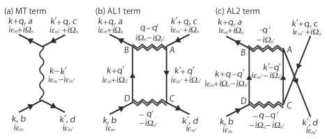
Figure 4: Diagrammatic representations of the irreducible four-point vertex functions in the FLEX approximation. Neglecting orbital indices and relabeling momentum and frequency variables, we can show that each diagram is equivalent to the corresponding diagram in Ref. Kon-CVC, .

Second, we carry out the analytic continuations of Eqs. (55), (56), and (57) to convert these into real-frequency representation. This is because the irreducible four-point vertex functions in real-frequency representation are necessary to calculate part of the kernel of the CVCs, $\mathcal{J}_{22;cdCD}^{(1)}(k,k^{\prime};0)$ [see Eq. (28)]. Carrying out the analytic continuations, we obtain the MT, the AL1, and the AL2 terms for regions 22-II, 22-III, and 22-IV (see Appendix F).

Third, using the MT, the AL1, and the AL2 terms in regions 22-II, 22-III, and 22-IV, we can calculate $\mathcal{J}_{22;cdCD}^{(1)}(k,k^{\prime};0)$ in the FLEX approximation. Since the irreducible four-point vertex function is the sum of the MT, the AL1, and the AL2 term, $\mathcal{J}_{22;cdCD}^{(1)}(k,k^{\prime};0)$ in the FLEX approximation is given by

$$\mathcal{J}_{22;abcd}^{(1)}(k,k^{\prime};0)= \mathcal{J}_{22;abcd}^{(1)\textrm{MT}}(k,k^{\prime};0)+\mathcal{J}_{22;abcd}^{(1)\textrm{AL}1}(k,k^{\prime};0)$$

$$+\mathcal{J}_{22;abcd}^{(1)\textrm{AL}2}(k,k^{\prime};0),$$ (61)

with

$$\mathcal{J}^{(1)\textrm{MT}}_{22;abcd}(k,k^{\prime};0)= \ F_{\textrm{ct}}^{\textrm{MT}}(\epsilon,\epsilon^{\prime};T)2i\textrm{Im}V_{acbd}^{(\textrm{R})}(k-k^{\prime}),$$ (62)

$$\mathcal{J}^{(1)\textrm{AL}1}_{22;abcd}(k,k^{\prime};0)= \ F_{\textrm{ct}}^{\textrm{AL}1}(\epsilon,\epsilon^{\prime};T)\Bigl{(}\frac{-i}{\pi}\Bigr{)}\frac{1}{N}\sum\limits_{\bm{q}^{\prime}}\sum\limits_{\{A\}}$$

$$\times\int^{\infty}_{-\infty}d\omega^{\prime}F_{\textrm{tt}}^{\textrm{AL}1}(\epsilon,\epsilon^{\prime},\omega^{\prime};T)$$

$$\times W^{\textrm{AL}(\textrm{RA})}_{aBcA;dCbD}(-q^{\prime};-q^{\prime})$$

$$\times\textrm{Im}G_{CA}^{(\textrm{R})}(k^{\prime}+q^{\prime})\textrm{Im}G_{BD}^{(\textrm{R})}(k+q^{\prime}),$$ (63)

and

$$\mathcal{J}^{(1)\textrm{AL}2}_{22;abcd}(k,k^{\prime};0)= \ F_{\textrm{ct}}^{\textrm{AL}2}(\epsilon,\epsilon^{\prime};T)\Bigl{(}\frac{-i}{\pi}\Bigr{)}\frac{1}{N}\sum\limits_{\bm{q}^{\prime}}\sum\limits_{\{A\}}$$

$$\times\int^{\infty}_{-\infty}d\omega^{\prime}F_{\textrm{tt}}^{\textrm{AL}2}(\epsilon,\epsilon^{\prime},\omega^{\prime};T)$$

$$\times W^{\textrm{AL}(\textrm{RA})}_{aBAd;CcbD}(-q^{\prime};-q^{\prime})$$

$$\times\textrm{Im}G_{AC}^{(\textrm{R})}(k^{\prime}-q^{\prime})\textrm{Im}G_{BD}^{(\textrm{R})}(k+q^{\prime}),$$ (64)

where $F_{\textrm{ct}}^{\textrm{MT}}(\epsilon,\epsilon^{\prime};T)$, $F_{\textrm{ct}}^{\textrm{AL}1}(\epsilon,\epsilon^{\prime};T)$, $F_{\textrm{tt}}^{\textrm{AL}1}(\epsilon,\epsilon^{\prime},\omega^{\prime};T)$, $F_{\textrm{ct}}^{\textrm{AL}2}(\epsilon,\epsilon^{\prime};T)$, and $F_{\textrm{tt}}^{\textrm{AL}2}(\epsilon,\epsilon^{\prime},\omega^{\prime};T)$ are, respectively,

$$F_{\textrm{ct}}^{\textrm{MT}}(\epsilon,\epsilon^{\prime};T)= \Bigl{(}\coth\frac{\epsilon-\epsilon^{\prime}}{2T}+\tanh\frac{\epsilon^{\prime}}{2T}\Bigr{)},$$ (65)

$$F_{\textrm{ct}}^{\textrm{AL}1}(\epsilon,\epsilon^{\prime};T)= \Bigl{(}\coth\frac{\epsilon^{\prime}-\epsilon}{2T}-\tanh\frac{\epsilon^{\prime}}{2T}\Bigr{)},$$ (66)

$$F_{\textrm{tt}}^{\textrm{AL}1}(\epsilon,\epsilon^{\prime},\omega^{\prime};T)= \Bigl{(}\tanh\frac{\omega^{\prime}+\epsilon}{2T}-\tanh\frac{\omega^{\prime}+\epsilon^{\prime}}{2T}\Bigr{)},$$ (67)

$$F_{\textrm{ct}}^{\textrm{AL}2}(\epsilon,\epsilon^{\prime};T)= \Bigl{(}\coth\frac{\epsilon^{\prime}+\epsilon}{2T}-\tanh\frac{\epsilon^{\prime}}{2T}\Bigr{)},$$ (68)

and

$$F_{\textrm{tt}}^{\textrm{AL}2}(\epsilon,\epsilon^{\prime},\omega^{\prime};T)=\Bigl{(}\tanh\frac{\omega^{\prime}+\epsilon}{2T}-\tanh\frac{\omega^{\prime}-\epsilon^{\prime}}{2T}\Bigr{)}.$$ (69)

In Eqs. (62)–(64), we have used the relations of the effective interaction and the single-particle Green’s functions due to the time-reversal and the even-parity symmetry; in more general case, we should not use the relations such as $V_{acbd}^{(\textrm{R})}(k-k^{\prime})-V_{acbd}^{(\textrm{A})}(k-k^{\prime})=2i\textrm{Im}V_{acbd}^{(\textrm{R})}(k-k^{\prime})$ and $G_{BD}^{(\textrm{R})}(k+q^{\prime})-G_{BD}^{(\textrm{A})}(k+q^{\prime})=2i\textrm{Im}G_{BD}^{(\textrm{R})}(k+q^{\prime})$, and should retain the differences between the retarded and the advanced quantities.

Fourth, substituting Eqs. (61) with Eqs. (62), (63), and (64) into Eq. (28), we obtain the following Bethe-Salpeter equation with the CVCs in the FLEX approximation:

$$\Lambda_{\nu;2;cd}(k;0)= \Lambda_{\nu;2;cd}^{(0)}(k;0)+\Delta\Lambda_{\nu;2;cd}^{\textrm{MT}}(k;0)$$

$$+\Delta\Lambda_{\nu;2;cd}^{\textrm{AL}1}(k;0)+\Delta\Lambda_{\nu;2;cd}^{\textrm{AL}2}(k;0),$$ (70)

where $\Delta\Lambda_{\nu;2;cd}^{\textrm{MT}}(k;0)$ is the MT CVC,

$$\Delta\Lambda_{\nu;2;cd}^{\textrm{MT}}(k;0)= \frac{1}{N}\sum\limits_{\bm{k}^{\prime}}\sum\limits_{\{A\}}\int^{\infty}_{-\infty}\frac{d\epsilon^{\prime}}{2\pi}F_{ct}^{\textrm{MT}}(\epsilon,\epsilon^{\prime};T)$$

$$\times\textrm{Im}V_{cCdD}^{(\textrm{R})}(k-k^{\prime})\tilde{\Lambda}_{\nu;2;CD}(k^{\prime};0),$$ (71)

$\Delta\Lambda_{\nu;2;cd}^{\textrm{AL}1}(k;0)$ is part of the AL CVC,

$$\Delta\Lambda_{\nu;2;cd}^{\textrm{AL}1}(k;0)= -\frac{1}{4\pi^{2}N^{2}}\sum\limits_{\bm{k}^{\prime},\bm{q}^{\prime}}\sum\limits_{\{A\}}\sum\limits_{\{A^{\prime\}}}\int^{\infty}_{-\infty}d\epsilon^{\prime}\int^{\infty}_{-\infty}d\omega^{\prime}$$

$$\times F_{\textrm{ct}}^{\textrm{AL}1}(\epsilon,\epsilon^{\prime};T)F_{\textrm{tt}}^{\textrm{AL}1}(\epsilon,\epsilon^{\prime},\omega^{\prime};T)$$

$$\times W^{\textrm{AL}(\textrm{RA})}_{cB^{\prime}CA^{\prime};DC^{\prime}dD^{\prime}}(-q^{\prime};-q^{\prime})$$

$$\times\textrm{Im}G_{C^{\prime}A^{\prime}}^{(\textrm{R})}(k^{\prime}+q^{\prime})\textrm{Im}G_{B^{\prime}D^{\prime}}^{(\textrm{R})}(k+q^{\prime})$$

$$\times\tilde{\Lambda}_{\nu;2;CD}(k^{\prime};0),$$ (72)

and $\Delta\Lambda_{\nu;2;cd}^{\textrm{AL}2}(k;0)$ is the other part of the AL CVC,

$$\Delta\Lambda_{\nu;2;cd}^{\textrm{AL}2}(k;0)= -\frac{1}{4\pi^{2}N^{2}}\sum\limits_{\bm{k}^{\prime},\bm{q}^{\prime}}\sum\limits_{\{A\}}\sum\limits_{\{A^{\prime\}}}\int^{\infty}_{-\infty}d\epsilon^{\prime}\int^{\infty}_{-\infty}d\omega^{\prime}$$

$$\times F_{\textrm{ct}}^{\textrm{AL}2}(\epsilon,\epsilon^{\prime};T)F_{\textrm{tt}}^{\textrm{AL}2}(\epsilon,\epsilon^{\prime},\omega^{\prime};T)$$

$$\times W^{\textrm{AL}(\textrm{RA})}_{cB^{\prime}A^{\prime}D;C^{\prime}CdD^{\prime}}(-q^{\prime};-q^{\prime})$$

$$\times\textrm{Im}G_{A^{\prime}C^{\prime}}^{(\textrm{R})}(k^{\prime}-q^{\prime})\textrm{Im}G_{B^{\prime}D^{\prime}}^{(\textrm{R})}(k+q^{\prime})$$

$$\times\tilde{\Lambda}_{\nu;2;CD}(k^{\prime};0),$$ (73)

with

$$\tilde{\Lambda}_{\nu;2;CD}(k^{\prime};0)= \sum\limits_{A,B}g_{2;CABD}(k^{\prime};0)\Lambda_{\nu;2;AB}(k^{\prime};0).$$ (74)

Equations (71)–(73) show that the MT and the AL CVC connect the currents at different momenta; for example, the MT CVC connects the current at $\bm{k}$ with the current at $\bm{k}^{\prime}$.

In the actual numerical calculations, instead of the above Bethe-Salpeter equation, I use the simplified Bethe-Salpeter equation where the AL CVC is simplified by only its main terms. The main terms of the AL CVC can be determined by using the following two properties satisfied in the present model: The terms arising from $U$ are dominant compared with the terms arising from the other interactions in a realistic parameter set (i.e., $U>U^{\prime}$, $U>J_{\textrm{H}}$, and $U>J^{\prime}$); the intraorbital components of the current are larger than the interorbital ones due to the large intraorbital hopping integrals compared with the interorbital hopping integrals (i.e., the larger intraorbital components of the group velocity). Namely, the main terms of the AL CVC are given by the sum of the following two quantities:

$$\Delta\Lambda_{\nu;2;cd}^{\textrm{AL}1}(k;0)= -\delta_{c,d}\frac{1}{4\pi^{2}N^{2}}\sum\limits_{\bm{k}^{\prime},\bm{q}^{\prime}}\int^{\infty}_{-\infty}d\epsilon^{\prime}\int^{\infty}_{-\infty}d\omega^{\prime}$$

$$\times F_{\textrm{ct}}^{\textrm{AL}1}(\epsilon,\epsilon^{\prime};T)F_{\textrm{tt}}^{\textrm{AL}1}(\epsilon,\epsilon^{\prime},\omega^{\prime};T)$$

$$\times W^{\textrm{AL}(\textrm{RA})}_{c}(-q^{\prime};-q^{\prime})$$

$$\times\textrm{Im}G_{cc}^{(\textrm{R})}(k^{\prime}+q^{\prime})\textrm{Im}G_{cc}^{(\textrm{R})}(k+q^{\prime})$$

$$\times\tilde{\Lambda}_{\nu;2;cc}(k^{\prime};0),$$ (75)

and

$$\Delta\Lambda_{\nu;2;cd}^{\textrm{AL}2}(k;0)= -\delta_{c,d}\frac{1}{4\pi^{2}N^{2}}\sum\limits_{\bm{k}^{\prime},\bm{q}^{\prime}}\int^{\infty}_{-\infty}d\epsilon^{\prime}\int^{\infty}_{-\infty}d\omega^{\prime}$$

$$\times F_{\textrm{ct}}^{\textrm{AL}2}(\epsilon,\epsilon^{\prime};T)F_{\textrm{tt}}^{\textrm{AL}2}(\epsilon,\epsilon^{\prime},\omega^{\prime};T)$$

$$\times W^{\textrm{AL}(\textrm{RA})}_{c}(-q^{\prime};-q^{\prime})$$

$$\times\textrm{Im}G_{cc}^{(\textrm{R})}(k^{\prime}-q^{\prime})\textrm{Im}G_{cc}^{(\textrm{R})}(k+q^{\prime})$$

$$\times\tilde{\Lambda}_{\nu;2;cc}(k^{\prime};0),$$ (76)

where $W^{\textrm{AL}(\textrm{RA})}_{c}(-q^{\prime};-q^{\prime})$ is given by

$$W^{\textrm{AL}(\textrm{RA})}_{c}(-q^{\prime};-q^{\prime})=\dfrac{3}{2}\tilde{N}_{cccc}^{\textrm{S}(\textrm{R})}(-q^{\prime})\tilde{N}_{cccc}^{\textrm{S}(\textrm{A})}(-q^{\prime})$$

$$+\dfrac{1}{2}\tilde{N}_{cccc}^{\textrm{C}(\textrm{R})}(-q^{\prime})\tilde{N}_{cccc}^{\textrm{C}(\textrm{A})}(-q^{\prime})-U^{2},$$ (77)

with

$$\tilde{N}_{cccc}^{\textrm{S}(\textrm{R})}(-q^{\prime})= \ U+U^{2}\chi_{cccc}^{\textrm{S}(\textrm{R})}(-q^{\prime}),$$ (78)

and

$$\tilde{N}_{cccc}^{\textrm{C}(\textrm{R})}(-q^{\prime})= \ U-U^{2}\chi_{cccc}^{\textrm{C}(\textrm{R})}(-q^{\prime}).$$ (79)

More precisely, by using the former of the above two properties (corresponding to considering only the terms arising from $U$), we can replace $W^{\textrm{AL}(\textrm{RA})}_{cB^{\prime}CA^{\prime};DC^{\prime}dD^{\prime}}(-q^{\prime};-q^{\prime})$ of the AL$1$ term and $W^{\textrm{AL}(\textrm{RA})}_{cB^{\prime}A^{\prime}D;C^{\prime}CdD^{\prime}}(-q^{\prime};-q^{\prime})$ of the AL$2$ term by, respectively, $\delta_{B^{\prime},c}\delta_{C,c}\delta_{A^{\prime},c}\delta_{D,d}\delta_{C^{\prime},d}\delta_{D^{\prime},d}W^{\textrm{AL}(\textrm{RA})}_{cccc;dddd}(-q^{\prime};-q^{\prime})$ and $\delta_{B^{\prime},c}\delta_{A^{\prime},c}\delta_{D,c}\delta_{C^{\prime},d}\delta_{C,d}\delta_{D^{\prime},d}W^{\textrm{AL}(\textrm{RA})}_{cccc;dddd}(-q^{\prime};-q^{\prime})$; furthermore, using the latter property, we obtain Eqs. (75) and (76). Solving Eqs. (70), (71), (75), and (76) with Eq. (27) self-consistently, we can determine the current including the CVCs arising from the self-energy and irreducible four-point vertex function in the FLEX approximation. I will describe the technical remarks to numerically solve those equations in Appendix G.

III Results

In this section, I show the results of the magnetic properties, the electronic structure, and the transport properties for a PM state of the multiorbital Hubbard model away from or near the AF QCP. In Sec. III A, I present the results of the magnetic properties in the FLEX approximation. From those results, we discuss the dominant fluctuations, the static and the dynamic properties of the spin susceptibility, the role of each $t_{2g}$ orbital, and the effects of the spin fluctuations on the imaginary part of the retarded effective interaction. In Sec. III B, to discuss the effects of the self-energy on the electronic structure, I show the results of the FS, the mass enhancement factor, the unrenormalized QP damping, and the QP damping in the FLEX approximation. In Sec. III C, we discuss the main effects of the AL CVC on the inplane resistivity, $\rho_{ab}$, and the Hall coefficient in the weak-field limit, $R_{\textrm{H}}$, in the FLEX approximation with the $\Sigma$ CVC, the MT CVC, and the main terms of the AL CVC and more simplified three cases. In addition to the temperature dependence of those transport coefficients, I show the orbital depedences of $\sigma_{xx}$ and $\lim\limits_{H\rightarrow 0}\frac{\sigma_{xy}}{H}$ in order to determine the role of each $t_{2g}$ orbital.

I obtained the results of this section by the numerical calculations using the techniques explained in Appendixes D and G and converting the quantities obtained in the FLEX approximation in Matsubara-frequency representation to the corresponding quantities in real-frequency representation by the Padé approximation Pade-approx ; Kusunose-Pade . In the numerical calculations, I used $N=64\times 64$ meshes and $M=1024$ Matsubara frequencies, set $\Delta\epsilon_{j}=\Delta\epsilon_{j^{\prime}}^{\prime}=\Delta\omega_{j^{\prime\prime}}^{\prime}=0.0025$ eV, $\epsilon_{\textrm{c}}=0.2$ eV, $J^{\prime}=J_{\textrm{H}}$, $U^{\prime}=U-2J_{\textrm{H}}$, and chose $J_{\textrm{H}}$, $U$, and $T$ as parameters. ($\Delta\epsilon_{j}$, $\Delta\epsilon_{j^{\prime}}^{\prime}$, and $\Delta\omega_{j^{\prime\prime}}^{\prime}$ are the intervals of the discretized real-frequency integrals, and $\epsilon_{\textrm{c}}$ is the cut-off frequency in the discretized real-frequency integrals.) The parameters of $J_{\textrm{H}}$, $U$, and $T$ were chosen as follows: I put $J_{\textrm{H}}=\frac{U}{6}$ except the analysis of the dominant fluctuation, in which the value of $J_{\textrm{H}}$ was chosen in the range of $0\leq J_{\textrm{H}}\leq\frac{U}{5}$; I considered the case of $U=1.8$ or $2.1$ eV as, respectively, case NA-review ; NA-CVC away from or near the AF QCP except the results in noninteracting case; I considered several values of $T$ in the range of $0.006\textrm{eV}\leq T\leq 0.03\textrm{eV}$. In addition, in the conversion by the Padé approximation, I numerically solved its recursive procedure Pade-approx ; Kusunose-Pade using the quantities at the lowest four Matsubara frequencies; for example, we obtained $\Sigma_{ab}^{(\textrm{R})}(\bm{k},\epsilon)$ by adopting that recursive procedure to a set of $\Sigma_{ab}(\bm{k},i\epsilon_{m})$ at $m=0,1,2,3$ in the FLEX approximation. Note that the advanced quantities are obtained by using the relations such as $\Sigma_{ab}^{(\textrm{A})}(\bm{k},\epsilon)=\Sigma_{ab}^{(\textrm{R})}(\bm{k},\epsilon)^{\ast}$ due to the time-reversal and the even-parity symmetries.

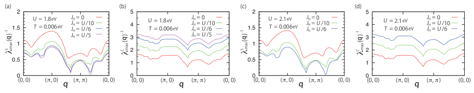
Figure 5: Momentum dependence of $\lambda^{\textrm{S}}_{\textrm{max}}(\bm{q})^{-1}$ and $\lambda^{\textrm{C}}_{\textrm{max}}(\bm{q})^{-1}$ at $T=0.006$ eV and $U=1.8$ and $2.1$ eV for several values of $J_{\textrm{H}}$.

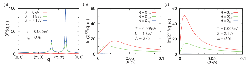
Figure 6: (a) Momentum dependence of $\chi^{\textrm{S}}(\bm{q},0)=\chi^{\textrm{S}(\textrm{R})}(\bm{q},0)$ at $T=0.006$ eV, $U=0$, $1.8$, and $2.1$ eV and $J_{\textrm{H}}=\frac{U}{6}$, and frequency dependence of $\textrm{Im}\chi^{\textrm{S}(\textrm{R})}(\bm{q},\omega)$ for $\bm{q}=\bm{Q}_{\textrm{IC-AF}}$, $\bm{Q}_{\textrm{IC-AF}}^{\prime}\equiv(\pi,\frac{21}{32}\pi)$, and $\bm{Q}_{\textrm{FM}}\equiv(0,0)$ at $T=0.006$ eV and $J_{\textrm{H}}=\frac{U}{6}$ for (b) $U=1.8$ eV and (c) $U=2.1$ eV.

III.1 Magnetic properties

In this section, I show four main results about the magnetic properties. First, the dominant fluctuations are the spin fluctuations. Second, an increase of electron correlation leads to the enhancement of low-energy spin fluctuation at $\bm{q}=\bm{Q}_{\textrm{IC-AF}}\equiv(\frac{21}{32}\pi,\frac{21}{32}\pi)$. Third, the diagonal and the nondiagonal component of $\chi_{aabb}^{\textrm{S}(\textrm{R})}(q)$ at $\bm{q}=\bm{Q}_{\textrm{IC-AF}}$ contribute to the enhancement of the spin fluctuation at $\bm{q}=\bm{Q}_{\textrm{IC-AF}}$, and the diagonal component of the $d_{xy}$ orbital is largest. Fourth, the orbital dependence of the effective interaction is determined by the orbital dependence of the spin fluctuation.

We first determine the dominant fluctuations in the present model. For that purpose, we analyze the effects of electron correlation on $\lambda^{\textrm{S}}_{\textrm{max}}(\bm{q})^{-1}$ and $\lambda^{\textrm{C}}_{\textrm{max}}(\bm{q})^{-1}$, the inverses of the maximum eigenvalues Tsunetsugu-RPA ; NA-RPA of $\chi_{abcd}^{\textrm{S}}(\bm{q},0)$ and $\chi_{abcd}^{\textrm{C}}(\bm{q},0)$, respectively. This is because by analyzing the dependence of $\lambda^{\textrm{S}}_{\textrm{max}}(\bm{q})^{-1}$ and $\lambda^{\textrm{C}}_{\textrm{max}}(\bm{q})^{-1}$ on $U$ and $J_{\textrm{H}}$, we can determine the dominant fluctuations among four kinds of fluctuations, i.e. charge fluctuations, spin fluctuations, orbital fluctuations, and spin-orbital-combined fluctuations Ueda-paramag ; NA-paramag (for more details see Appendix H). I show $\lambda^{\textrm{S}}_{\textrm{max}}(\bm{q})^{-1}$ and $\lambda^{\textrm{C}}_{\textrm{max}}(\bm{q})^{-1}$ at $T=0.006$ eV and $U=1.8$ eV for several values of $J_{\textrm{H}}$ in Figs. 5(a) and 5(b), respectively. We see that as $J_{\textrm{H}}$ increases, $\lambda^{\textrm{S}}_{\textrm{max}}(\bm{q})^{-1}$ monotonically decreases, and $\lambda^{\textrm{C}}_{\textrm{max}}(\bm{q})^{-1}$ monotonically increases. This behavior is characteristic of the enhancement of spin fluctuations and the suppression of the charge fluctuations Ueda-paramag ; NA-paramag (see Appendix H). The similar results are obtained at $U=2.1$ eV, as shown in Figs. 5(c) and 5(d). Since approaching the inverse of the maximum eigenvalue towards zero characterizes the enhancement of the susceptibility, the results in Figs. 5(a)–5(d) show that spin fluctuations are dominant at $U=1.8$ and $2.1$ eV in the present model. This can be understood by considering the following three facts: the noninteracting susceptibility for $a=c$ and $b=d$, $\chi_{abab}^{(0)}(\bm{q},i\Omega_{n})$, becomes very large in the present model since $G_{aa}^{(0)}(\bm{k},i\omega_{m})$ is larger than $G_{ab}^{(0)}(\bm{k},i\omega_{m})$ for $b\neq a$ due to the large intraorbital hopping integrals compared with the interorbital ones; the interactions between the different kinds of fluctuations may be generally very weak in the FLEX approximation due to lack of the vertex corrections of the susceptibilities; the terms arising from $U$ cause the strongest enhancement of the susceptibilities. Namely, due to those facts, the intraorbital components of $\chi_{abcd}^{\textrm{S}}(\bm{q},i\Omega_{n})$, i.e. $\chi_{aaaa}^{\textrm{S}}(\bm{q},i\Omega_{n})$, are strongly enhanced, resulting in the larger enhancement of spin fluctuations than the other fluctuations. Hereafter, we fix the value of $J_{\textrm{H}}$ at $J_{\textrm{H}}=\frac{U}{6}$.

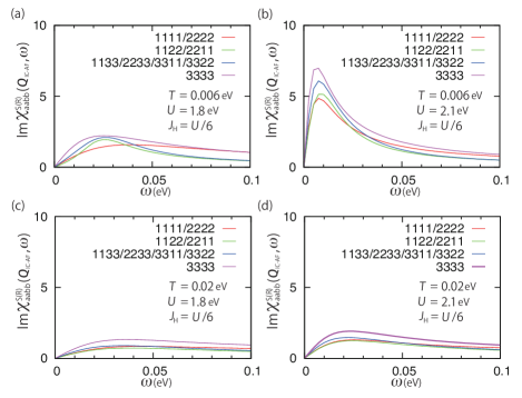
Figure 7: Frequency dependence of $\textrm{Im}\chi^{\textrm{S}(\textrm{R})}_{aabb}(\bm{Q}_{\textrm{IC-AF}},\omega)$ at $J_{\textrm{H}}=\frac{U}{6}$ for $(T,U)=$(a)$(0.006,1.8)$, (b)$(0.006,2.1)$, (c)$(0.02,1.8)$, and (d)$(0.02,2.1)$ (eV).

Then, for a deeper understanding of spin fluctuations in the present model, I analyze the static and the dynamic properties of the spin susceptibility as a function of $\omega$, $\chi^{\textrm{S}(\textrm{R})}(\bm{q},\omega)=\sum_{a,b}\chi^{\textrm{S}(\textrm{R})}_{aabb}(\bm{q},\omega)$. For the analysis of the static property, I show the momentum dependence of $\chi^{\textrm{S}}(\bm{q},0)=\chi^{\textrm{S}(\textrm{R})}(\bm{q},0)$ at $T=0.006$ eV for $U=1.8$ and $2.1$ eV in Fig. 6(a). The result shows that as $U$ increases, the spin fluctuation at $\bm{q}=\bm{Q}_{\textrm{IC-AF}}$ is most strongly enhanced and the enhancement at $\bm{q}=(0,0)$ is much weaker. That strongest enhancement can be understood as the combination of the merging of the nesting vectors of the $d_{xz/yz}$ and $d_{xy}$ orbitals around $\bm{q}=\bm{Q}_{\textrm{IC-AF}}$ due to the mode-mode coupling for the spin fluctuations around $\bm{q}=\bm{Q}_{\textrm{IC-AF}}$ and the nesting instability at $\bm{q}=\bm{Q}_{\textrm{IC-AF}}$ due to the RPA-type scattering process, as explained in Ref. NA-CVC, . Next, for the analysis of the dynamic property, I show the frequency dependence of $\textrm{Im}\chi^{\textrm{S}(\textrm{R})}(\bm{q},\omega)$ for several values of $\bm{q}$ at $T=0.006$ eV for $U=1.8$ and $2.1$ eV in Figs. 6(b) and 6(c). These figures show that low-energy spin fluctuation at $\bm{q}=\bm{Q}_{\textrm{IC-AF}}$ is dominant in the dynamic properties at $U=1.8$ and $2.1$ eV, and that the intensity at $\bm{q}=(0,0)$ is very small.

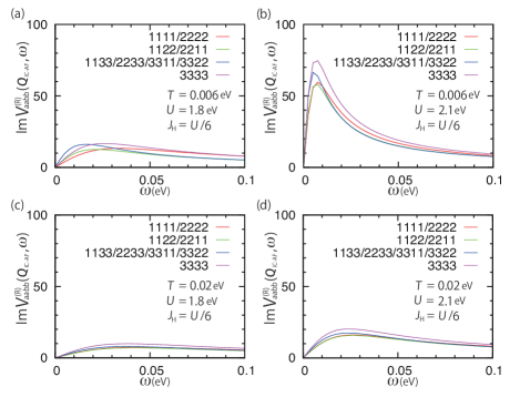
Figure 8: Frequency dependence of $\textrm{Im}V^{(\textrm{R})}_{aabb}(\bm{Q}_{\textrm{IC-AF}},\omega)$ at $J_{\textrm{H}}=\frac{U}{6}$ for $(T,U)=$(a)$(0.006,1.8)$, (b)$(0.006,2.1)$, (c)$(0.02,1.8)$, and (d)$(0.02,2.1)$ (eV).

Moreover, I analyze the role of each $t_{2g}$ orbital in discussing the spin fluctuations. Figures 7(a)–7(d) show the frequency dependences of $\textrm{Im}\chi_{aabb}^{\textrm{S}(\textrm{R})}(\bm{Q}_{\textrm{IC-AF}},\omega)$ at $J_{\textrm{H}}=\frac{U}{6}$ for $(T,U)=(0.006,1.8)$, $(0.006,2.1)$, $(0.02,1.8)$, and $(0.02,2.1)$ (eV). We see that not only the diagonal but also the non-diagonal components are enhanced, and that the largest component is the diagonal one of the $d_{xy}$ orbital. First, the enhancement of the diagonal components arises from the combination of the large diagonal components of the noninteracting susceptibility of the $t_{2g}$ orbitals around $\bm{q}=\bm{Q}_{\textrm{IC-AF}}$, the merging of the nesting vectors of the $d_{xz/yz}$ and the $d_{xy}$ orbital around $\bm{q}=\bm{Q}_{\textrm{IC-AF}}$, and the larger enhancement due to the terms arising from $U$ than the other terms. Next, the nondiagonal components are enhanced due to the terms including $J_{\textrm{H}}$ and the diagonal components since $\chi_{aabb}^{\textrm{S}}(\bm{q},i\Omega_{n})$ for $a\neq b$ are enhanced mainly through $\chi_{aaaa}(\bm{q},i\Omega_{n})U\chi_{aabb}^{\textrm{S}}(\bm{q},i\Omega_{n})+\chi_{aaaa}(\bm{q},i\Omega_{n})J_{\textrm{H}}\chi_{bbbb}^{\textrm{S}}(\bm{q},i\Omega_{n})$ [see the second term of Eq. (45)]. Then, the diagonal component of the $d_{xy}$ orbital becomes largest due to the following three properties: the diagonal components of the noninteracting susceptibility are larger than the non-diagonal components due to the large intraorbital hopping integrals; the noninteracting susceptibility of the $d_{xy}$ orbital is larger than that of the $d_{xz/yz}$ orbital due to the larger DOS NA-review of the $d_{xy}$ orbital; the enhancement due to the terms arising from $U$ is largest in the terms arising from the Hubbard interaction terms.

Finally, we see the effect of the spin fluctuations on the imaginary part of the retarded effective interaction of the FLEX approximation. The reason why that effect is analyzed is that its understanding is useful to understand the effect of the spin fluctuations on the MT CVC since the imaginary part of the retarded effective interaction is part of the kernel of the MT CVC [see Eq. (71)]. For that analysis, it is sufficient to present $\textrm{Im}V_{aabb}^{(\textrm{R})}(\bm{q},\omega)$ since the other orbital components are much less important. This is due to the facts that the dominant fluctuations are the spin fluctuations and that their contributions to the effective interaction, $V_{acbd}(\bm{q},i\Omega_{n})$, are given by $\textstyle\sum_{A,C}U_{acAA}^{\textrm{S}}\chi_{AACC}^{\textrm{S}}(\bm{q},i\Omega_{n})U_{CCbd}^{\textrm{S}}=\delta_{a,c}\delta_{b,d}\textstyle\sum_{A,C}U_{aaAA}^{\textrm{S}}\chi_{AACC}^{\textrm{S}}(\bm{q},i\Omega_{n})U_{CCbb}^{\textrm{S}}$ [see Eq. (51)]. Figures 8(a)–8(d) show the frequency dependence of $\textrm{Im}V_{aabb}^{(\textrm{R})}(\bm{Q}_{\textrm{IC-AF}},\omega)$ for $(T,U)=(0.006,1.8)$, $(0.006,2.1)$, $(0.02,1.8)$, and $(0.02,2.1)$ (eV). The obtained orbital dependence is similar to that for $\textrm{Im}\chi_{aabb}^{\textrm{S}(\textrm{R})}(\bm{q},\omega)$. Thus, the spin fluctuations lead to the main contributions to the MT CVC in the present model, and the orbital dependence of the MT CVC is determined by the orbital dependence of the spin fluctuations.

III.2 Electronic structure

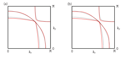
Figure 9: FSs at $T=0.006$ eV and $J_{\textrm{H}}=\frac{U}{6}$ for (a) $U=1.8$ eV and (b) $U=2.1$ eV. In panels (a) and (b), the FS sheets at $U=0$ eV are shown by the dotted lines for comparison.

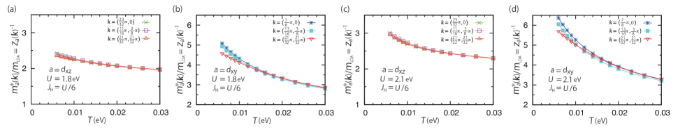
Figure 10: Temperature dependence of $z_{a}(\bm{k})^{-1}=1-\frac{\partial\textrm{Re}\Sigma_{aa}^{(\textrm{R})}(\bm{k},\omega)}{\partial\omega}|_{\omega\rightarrow 0}$ for several $\bm{k}$ at $J_{\textrm{H}}=\frac{U}{6}$ for (a) $a=d_{xz}$ and $U=1.8$ eV, (b) $a=d_{xy}$ and $U=1.8$ eV, (c) $a=d_{xz}$ and $U=2.1$ eV, and (d) $a=d_{xy}$ and $U=2.1$ eV. $z_{d_{yz}}(\bm{k})^{-1}$ is given by $z_{d_{yz}}(k_{x},k_{y})^{-1}=z_{d_{xz}}(k_{y},k_{x})^{-1}$.

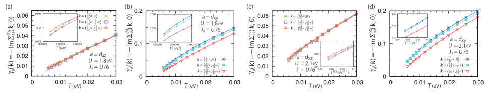
Figure 11: Temperature dependence of $\gamma_{a}(\bm{k})=-\textrm{Im}\Sigma_{aa}^{(\textrm{R})}(\bm{k},0)$ for several $\bm{k}$ at $J_{\textrm{H}}=\frac{U}{6}$ for (a) $a=d_{xz}$ and $U=1.8$ eV, (b) $a=d_{xy}$ and $U=1.8$ eV, (c) $a=d_{xz}$ and $U=2.1$ eV, and (d) $a=d_{xy}$ and $U=2.1$ eV. The inset in panel (a) or (b) shows $\gamma_{a}(\bm{k})$ against $T^{2}$ below $T=0.01$ eV, and the inset in panel (c) or (d) shows $\gamma_{a}(\bm{k})$ against $T^{0.5}$ below $T=0.01$ eV. $\gamma_{d_{yz}}(\bm{k})$ is given by $\gamma_{d_{yz}}(k_{x},k_{y})=\gamma_{d_{xz}}(k_{y},k_{x})$.

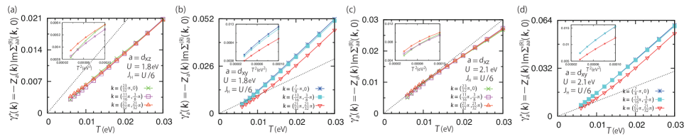
Figure 12: Temperature dependence of $\gamma_{a}^{\ast}(\bm{k})=z_{a}(\bm{k})\gamma_{a}(\bm{k})$ for several $\bm{k}$ at $J_{\textrm{H}}=\frac{U}{6}$ for (a) $a=d_{xz}$ and $U=1.8$ eV, (b) $a=d_{xy}$ and $U=1.8$ eV, (c) $a=d_{xz}$ and $U=2.1$ eV, and (d) $a=d_{xy}$ and $U=2.1$ eV. $\gamma_{a}^{\ast}(\bm{k})=T$ are shown by the dotted lines to discuss whether the QP damping is cold-spot-type or hot-spot-type, and the insets show $\gamma_{a}^{\ast}(\bm{k})$ against $T^{2}$ below $T=0.01$ eV. $\gamma_{d_{yz}}^{\ast}(\bm{k})$ is given by $\gamma_{d_{yz}}^{\ast}(k_{x},k_{y})=\gamma_{d_{xz}}^{\ast}(k_{y},k_{x})$.

In this section, I show four main results about the electronic structure. First, the topology of the FS remains the same as the noninteracting one even including the FS deformation due to the real part of the self-energy in the FLEX approximation. Second, the mass enhancement of the $d_{xy}$ orbital is larger than that of the $d_{xz/yz}$ orbital in a wide region of the parameter space in the present model. Third, the unrenormalized QP damping of the $d_{xy}$ orbital becomes larger than that of the $d_{xz/yz}$ orbital. Fourth, the orbital dependence of the QP damping is mainly determined by the orbital dependence of the unrenormalized QP damping.

I begin with the effects of the real part of the self-energy in the FLEX approximation on the FS and the mass enhancement factor. I determine the FS by diagonalizing $[\epsilon_{ab}(\bm{k})+\textrm{Re}\Sigma_{ab}^{(\textrm{R})}(\bm{k},0)]$, where $\mu$ in $\epsilon_{ab}(\bm{k})$ has been determined by Eq. (52).

First, we see from Figs. 9(a) and 9(b) how the FS is modified with increasing $U$. Those figures show that the modification is slight. Thus, the real part of the self-energy in the FLEX approximation does not change the topology of the FS sheets (i.e., whether each sheet is electron-like or hole-like). This result can be understood by considering two facts that the occupation numbers of the $d_{xz/yz}$ and the $d_{xy}$ orbital do not become very close to integers, and that the van Hove singularity of the $d_{xy}$ orbital does not cross over the Fermi level. Note, first, that the occupation numbers of the $d_{xz/yz}$ and the $d_{xy}$ orbitals are $1.36$ and $1.28$, respectively, at $U=1.8$ and $2.1$ eV; second, that if the van Hove singularity crosses over the Fermi level, the $\gamma$ sheet touches the boundary of the Brillouin zone at $\bm{k}=(\pi,0)$ or $(0,\pi)$.

Next, we show the mass enhancement factor, $z_{a}(\bm{k})^{-1}=1-\frac{\partial\textrm{Re}\Sigma_{aa}^{(\textrm{R})}(\bm{k},\omega)}{\partial\omega}|_{\omega\rightarrow 0}$, at $U=1.8$ and $2.1$ eV in Figs. 10(a)–10(d). From those figures, we find three properties about the orbital, temperature, and momentum dependences of $z_{a}(\bm{k})^{-1}$. The first property is that the mass enhancement of the $d_{xy}$ orbital is always larger than that of the $d_{xz/yz}$ orbital for all the temperatures considered. This arises from the stronger spin fluctuations of the $d_{xy}$ orbital than those of the $d_{xz/yz}$ orbital, as explained in Ref. NA-CVC, . Combining this result with the similar orbital dependence NA-CVC of $z_{a}(\bm{k})^{-1}$ as a function of $J_{\textrm{H}}$ (in $0\leq J_{\textrm{H}}\leq\frac{U}{5}$ at $T=0.006$ eV and $U=1.8$ eV), we deduce that the larger mass enhancement of the $d_{xy}$ orbital is realized in a wide region of the parameter space of the present model for a PM state in the FLEX approximation. It should be noted that although the spin fluctuations of the $d_{xy}$ orbital enhance $z_{a}(\bm{k})^{-1}$ of not only the $d_{xy}$ orbital but also the $d_{xz/yz}$ orbital, the enhancement for the $d_{xy}$ is larger in a realistic set of the Hubbard interaction terms. This is because the spin fluctuations of an orbital cause the enhancement of $z_{a}(\bm{k})^{-1}$ of the orbital proportional to the $U^{2}$ terms of $\frac{3}{2}\textstyle\sum_{A,B}U_{aaAA}^{\textrm{S}}\chi_{AABB}^{\textrm{S}}(\bm{q},i\Omega_{n})U_{BBaa}^{\textrm{S}}$ in $V_{aaaa}(\bm{q},i\Omega_{n})$ in $\Sigma_{aa}(\bm{k},i\epsilon_{m})$, and the enhancement of $z_{a}(\bm{k})^{-1}$ of another orbital proportional to the $J_{\textrm{H}}^{2}$ terms. Then, the second property found in Figs. 10(a)–10(d) is that the temperature dependence is weak other than the case for the $d_{xy}$ orbital at $U=2.1$ eV. This results from the more significant enhancement of the spin fluctuations of the $d_{xy}$ orbital with decreasing temperature [see Figs. 7(a)–7(d)], and suggests that the mass enhancement of the $d_{xy}$ orbital may remain larger even at lower temperatures than the temperatures considered. The third property of Figs. 10(a)–10(d) is that the momentum dependence is negligible for the $d_{xz/yz}$ orbital, while the $d_{xy}$ orbital has the weak momentum dependence. This is due to the difference between the quasi-one-dimensionality of the $d_{xz/yz}$ orbital and the quasi-two-dimensionality of the $d_{xy}$ orbital: only the $d_{xy}$ orbital has the van Hove singularity due to the saddle points at $\bm{k}\approx(\frac{23}{32}\pi,0)$ and $(0,\frac{23}{32}\pi)$, resulting in a larger mass enhancement vHs-cuprate . Since this result shows that the momentum dependence of the mass enhancement factor is not important to discuss the magnitude difference of the mass enhancement, the present analysis is sufficient for that discussion.

Then, we turn to the effects of the imaginary of the self-energy on the unrenormalized QP damping, $\gamma_{a}(\bm{k})=-\textrm{Im}\Sigma_{aa}^{(\textrm{R})}(\bm{k},0)$. From the results shown in Figs. 11(a)–11(d), we see three main features. The first one is about the orbital dependence: the magnitude for the $d_{xy}$ orbital is about three times as large as that for the $d_{xz/yz}$ orbital. This arises mainly from the larger DOS and stronger spin fluctuations of the $d_{xy}$ orbital. Note, first, that a ratio of the noninteracting DOSs of the $d_{xy}$ and the $d_{xz/yz}$ orbitals on the Fermi level is about $2.3$ NA-review ; second, that due to the similar reasons for $z_{a}(\bm{k})^{-1}$, the spin fluctuations of the $d_{xy}$ orbital cause a larger enhancement of $\gamma_{a}(\bm{k})$ of the $d_{xy}$ orbital in a realistic set of the Hubbard interaction terms. The second main feature is about the temperature dependence: the unrenormalized QP dampings of the $d_{xz/yz}$ orbital at $U=1.8$ eV show the $T^{2}$ dependence at low temperatures; the $T^{0.5}$ dependence of $\gamma_{a}(\bm{k})$ for the $d_{xz/yz}$ orbital is realized for $\bm{k}=(\frac{21}{32}\pi,\frac{21}{32}\pi)$ at $U=2.1$ eV; the unrenormalized QP damping of the $d_{xy}$ orbital at $\bm{k}=(\frac{7}{8}\pi,0)$ is proportional to $T$ linear at $U=1.8$ and $2.1$ eV. The $T^{2}$ dependence is due to the formation of long-lived QPs AGD ; the $T^{0.5}$ dependence results from the hot-spot structure Hlubina-Rice due to the enhanced AF spin fluctuation, as explained in Ref. NA-review, ; the $T$-linear behavior emerges as a result of the existence of the van Hove singularity Hlubina-Rice . The third main feature is about the momentum dependence: the unrenormalized QP damping of the $d_{xy}$ orbital depends weakly on momentum; the momentum dependence for the $d_{xz/yz}$ orbital is negligible. This arises from the considerable difference in the momentum dependence of the single-particle spectrum function due to the existence of the van Hove singularity only for the $d_{xy}$ orbital.

Finally, we analyze the effects of the combination of the real and the imaginary part of the self-energy on the QP damping, $\gamma_{a}^{\ast}(\bm{k})=z_{a}(\bm{k})\gamma_{a}(\bm{k})$. From the results shown in Figs. 12(a)–12(d), we see that even for the QP damping, the larger magnitude for the $d_{xy}$ orbital is realized. This is due to the larger difference in the unrenormalized QP damping compared with the difference in the mass enhancement factor, and suggests that the QPs of the $d_{xz/yz}$ orbital are more coherent than the QPs of the $d_{xy}$ orbital in the present model. In addition, we find the $T^{2}$ dependence for the $d_{xz/yz}$ orbital at low temperatures at $U=1.8$ eV, the deviation from the $T^{2}$ dependence for the $d_{xz/yz}$ orbital at $U=2.1$ eV, and the similar momentum dependence of the QP damping to that of the unrenormalized QP damping.

III.3 Transport properties

In this section, I show three main results about the transport properties. First, the main results in the previous studies NA-review ; NA-CVC remain qualitatively unchanged even including the main terms of the AL CVC. Second, the temperature dependences of $\rho_{ab}$ and $R_{\textrm{H}}$ near the AF QCP consist of two regions, high-temperature region, where only the $\Sigma$ CVC is sufficient, and low-temperature region, where only both the $\Sigma$ CVC and the MT CVC are sufficient. Third, in contrast to the case near the AF QCP, the effects of the MT CVC on $\rho_{ab}$ and $R_{\textrm{H}}$ at low temperatures are different in case away from the AF QCP: only for $R_{\textrm{H}}$, the effects are considerable.

To analyze the main effects of the AL CVC on $\rho_{ab}$ and $R_{\textrm{H}}$, we consider four cases, named MT$+$AL CVC case, MT CVC case, $\Sigma$ CVC case, and No CVC case. In the MT$+$AL CVC case, we take account of the $\Sigma$ CVC, the MT CVC, and the main terms of the AL CVC: $\Lambda_{\nu;2;cd}(k;0)$ in Eq. (70) includes those CVCs, and $\Lambda_{\nu;2;ab}^{(0)}(k;0)$ in Eq. (27) includes the $\Sigma$ CVC. In the MT CVC, we neglect only the AL CVC and take account of the other CVCs: the change from the MT$+$AL CVC case is neglecting the AL CVC in $\Lambda_{\nu;2;cd}(k;0)$. In the $\Sigma$ CVC case, we take account of only the $\Sigma$ CVC among the CVCs: $\Lambda_{\nu;2;cd}(k;0)$ becomes the same as $\Lambda_{\nu;2;ab}^{(0)}(k;0)$. In the No CVC case, we neglect all the CVCs: $\Lambda_{\nu;2;cd}(k;0)$ and $\Lambda_{\nu;2;ab}^{(0)}(k;0)$ are determined only by the noninteracting group velocity.

III.3.1 In-plane resistivity

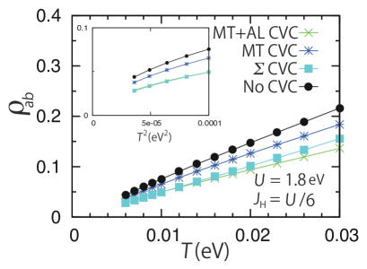
Figure 13: Temperature dependence of $\rho_{ab}$ at $U=1.8$ eV and $J_{\textrm{H}}=\frac{U}{6}$ in the four cases. The inset shows $\rho_{ab}$ against $T^{2}$ below $T=0.01$ eV.

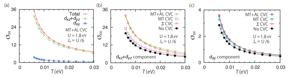
Figure 14: Temperature dependence of (a) $\sigma_{xx}$ and orbital-decomposed components in the MT$+$AL CVC case at $U=1.8$ eV and the orbital-decomposed components of (b) the $d_{xz}$ and $d_{yz}$ orbitals and (c) $d_{xy}$ orbital in the four cases at $U=1.8$ eV.

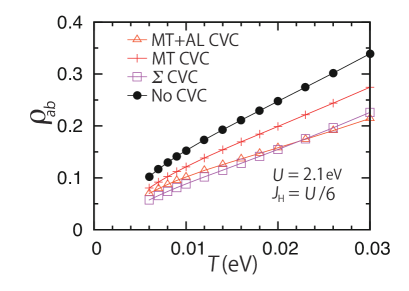
Figure 15: Temperature dependence of $\rho_{ab}$ at $U=2.1$ eV and $J_{\textrm{H}}=\frac{U}{6}$ in the four cases.

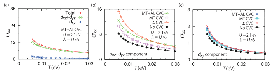
Figure 16: Temperature dependence of (a) $\sigma_{xx}$ and orbital-decomposed components in the MT$+$AL CVC case at $U=2.1$ eV and the orbital-decomposed components of (b) the $d_{xz}$ and $d_{yz}$ orbitals and (c) $d_{xy}$ orbital in the four cases at $U=2.1$ eV.

We begin with $\rho_{ab}(=\sigma_{xx}^{-1}=\sigma_{yy}^{-1})$ away from the AF QCP. We show the temperature dependence of $\rho_{ab}$ at $U=1.8$ eV in the four cases in Fig. 13, and find two main features. One is that the $T^{2}$ dependence below $T=0.008$ eV holds even in the MT$+$AL CVC case. This can be understood that the CVCs little affect the power of the temperature dependence of the resistivity. This is because the main effects of the CVCs on the resistivity arise from the magnitude changes of the current [see Sect. II B 1] and because the magnitude changes appear in the equation of the resistivity as $\frac{1}{|\Lambda_{2;cd}^{(0)}(k)|+\Delta|\Lambda_{2;cd}(k)|}\sim\frac{1}{|\Lambda_{2;cd}^{(0)}(k)|}(1-\frac{\Delta|\Lambda_{2;cd}(k)|}{|\Lambda_{2;cd}^{(0)}(k)|})$, where $\frac{\Delta|\Lambda_{2;cd}(k)|}{|\Lambda_{2;cd}^{(0)}(k)|}$ is not large. The other main feature is that the value of $\rho_{ab}$ in the MT$+$AL CVC case becomes smaller than that in the MT CVC case and nearly the same as that in the $\Sigma$ CVC case. This is due to the small effects of the MT and the AL CVC; for high-temperature region, the small effects arise from the dominance of the QP damping compared with the spin susceptibility in determining the kernels of those CVCs; for low-temperature region, the small effects arise from the combination of the not large spin susceptibility and the partial cancellation between the effects of the MT and the AL CVC. The more detailed explanations about those are as follows: In discussing the effects of the MT and the AL CVC, the relative values of the spin susceptibility and the QP damping are important since the kernels of the MT and the AL CVC contain the spin susceptibility and the inverse of the QP damping [see Eqs. (70)–(73)]. Due to this property, at high temperatures, the kernels become small since the QP damping is large; thus, the effects of the MT and the AL CVC are small for high-temperature region. Furthermore, although the effects of the MT and the AL CVC are separately non-negligible at low temperatures since with decreasing temperature the QP damping decreases and the spin susceptibility remains almost unchanged, the effects of the AL CVC reduce the effects of the MT CVC as a result of the difference in the momentum dependence; due to this reduction, the total effects of the MT and the AL CVC are small. Such property due to the difference in the momentum dependence can be easily seen from a simple and sufficient case of the second-order perturbation theory for a single-orbital system since the momentum structure of each diagram of the MT, AL1, and AL2 terms remains the same as in the FLEX approximation: in this case, the MT CVC is given by $\textstyle\sum_{\bm{k}^{\prime},\bm{q}}\Delta_{0}(\bm{k},\bm{k}^{\prime};\bm{k}^{\prime}+\bm{q},\bm{k}-\bm{q})\bm{\Phi}_{\bm{k}-\bm{q}}(\epsilon)$, and the AL1 and AL2 CVCs are $\textstyle\sum_{\bm{k}^{\prime},\bm{q}}\Delta_{0}(\bm{k},\bm{k}^{\prime};\bm{k}^{\prime}+\bm{q},\bm{k}-\bm{q})[\bm{\Phi}_{\bm{k}^{\prime}+\bm{q}}(\epsilon)-\bm{\Phi}_{\bm{k}^{\prime}}(\epsilon)]$ (for more details, see Ref. Yamada-Yosida, ); since $\bm{\Phi}_{\bm{k}}(\epsilon)$ is odd about momentum, the difference in the sign of $\bm{q}$ leads to the partial cancellation of the effects of the MT and the AL CVC.

We next discuss the role of each $t_{2g}$ orbital in determining $\rho_{ab}$ away from the AF QCP. For that purpose, I show the orbital-decomposed components of $\sigma_{xx}$, the $d_{xz}+d_{yz}$ component and the $d_{xy}$ component; the former is obtained by replacing $\textstyle\sum_{\{a\}=1}^{3}$ in Eq. (26) by $\textstyle\sum_{\{a\}=1}^{2}$, and the latter is obtained by replacing $\textstyle\sum_{\{a\}=1}^{3}$ in Eq. (26) by $\textstyle\sum_{\{a\}=3}$. As explained in Ref. NA-review, , only those components are sufficient in the present model since those (diagonal) components are larger than the non-diagonal ones due to the large intraorbital hopping integrals compared with the interorbital hopping integrals. First, we see from Fig. 14(a) that $\sigma_{xx/yy}$ is determined almost by the component of the $d_{xz/yz}$ orbital, and that the contributions from the component of the $d_{xy}$ orbital are very small. Namely, the $d_{xz}+d_{yz}$ component remains dominant even with the main terms of the AL CVC. We also see from Figs. 14(b) and 14(c) that the values in the MT$+$AL CVC case are nearly the same in the $\Sigma$ CVC case. Thus, the $\Sigma$ CVC is sufficient for discussions about the orbital dependence away from the AF QCP.

From the results at $U=1.8$ eV, we deduce, first, that the main results obtained in the previous studies NA-review ; NA-CVC away from the AF QCP, the $T^{2}$ dependence of $\rho_{ab}$ at low temperatures and the dominance of the $d_{xz/yz}$ orbital, remain qualitatively the same even with the main terms of the AL CVC; second, that the resistivity away from the AF QCP can be almost well described by taking account of only the $\Sigma$ CVC.

Then, I turn to $\rho_{ab}$ near the AF QCP. From its temperature dependence shown in Fig. 15, we see three main features about $\rho_{ab}$ in the MT$+$AL CVC case. First, $\rho_{ab}$ in the MT$+$AL CVC case shows the $T$-linear dependence, which is similar for the other three cases. This origin is the same for the other three cases NA-review ; NA-CVC , i.e. the $T^{0.5}$ dependence of the unrenormalized QP damping of the $d_{xz/yz}$ orbital around $\bm{k}=(\frac{21}{32}\pi,\frac{21}{32}\pi)$, since the CVCs little affect the power of the temperature dependence of $\rho_{ab}$ and since the $d_{xz}+d_{yz}$ component remains dominant even with the main terms of the AL CVC [see Fig. 16(a)]. Second, the values of $\rho_{ab}$ in the MT$+$AL CVC case at high temperatures are nearly the same as those in the $\Sigma$ CVC case at the corresponding temperatures. This is due to the same reason as that away from the AF QCP. Third, as temperature decreases, the value of $\rho_{ab}$ in the MT$+$AL CVC case approaches the value in the MT CVC case. This can be understood by combining two facts that the MT and the AL CVCs separately becomes non-negligible at low temperatures, and that the AL CVC near the AF QCP is negligible compared with the MT CVC in the presence of the even-parity symmetry and rotational symmetry. The mechanism of the former fact explained above, and the mechanism of the latter explained by the authors of Ref. Kon-CVC, . The explanations about the latter are as follows: When the system approaches an AF QCP characterized by spin fluctuation at $\bm{q}=\bm{Q}_{\textrm{QCP}}$, that spin fluctuation gives the leading contributions to the MT, AL$1$, and AL$2$ CVCs through $\textrm{Im}V_{cCdD}^{(\textrm{R})}(k-k^{\prime})$ in Eq. (71) and $W^{\textrm{AL}(\textrm{RA})}_{c}(-q^{\prime};-q^{\prime})$ in Eqs. (75) and (76), respectively. Then, although the MT CVC becomes more important near the AF QCP, the AL$1$ and AL$2$ CVCs become little important compared with the MT CVC near the AF QCP due to the cancellation between the contributions from $\bm{k}^{\prime}$ and $-\bm{k}^{\prime}$ arising from the spin fluctuation at $\bm{q}=\bm{Q}_{\textrm{QCP}}$. This cancellation is because in the terms of the AL$1$ or AL$2$ CVC only $\tilde{\Lambda}_{\nu;2;cc}(k^{\prime};0)$ is odd about momentum (i.e., the others are even) due to the even-parity symmetry and because the states at $-\bm{k}^{\prime}+\bm{Q}_{\textrm{QCP}}$ and $-\bm{k}^{\prime}-\bm{Q}_{\textrm{QCP}}$ are equivalent due to the rotational symmetry.

Moreover, we determine the role of each $t_{2g}$ orbital in determining $\rho_{ab}$ near the AF QCP from the results of the orbital-decomposed components of $\sigma_{xx}$. Figure 16(a) shows that the main terms of the AL CVC keep the dominance of the $d_{xz}+d_{yz}$ component unchanged. Furthermore, from Figs. 16(b) and 16(c), we see a similar behavior for $\rho_{ab}$ at low temperatures, i.e. an approach of the value of the $d_{xz}+d_{yz}$ component or the $d_{xy}$ component in the MT$+$AL CVC case towards that in the MT CVC case with decreasing temperature.

Combining the results at $U=2.1$ eV, we find that the $T$-linear $\rho_{ab}$ and the dominance of the $d_{xz/yz}$ orbital which are obtained in the MT CVC case are qualitatively unchanged even in the MT$+$AL CVC case, and that there are two almost distinct regions of the temperature dependence of $\rho_{ab}$. Those regions consist of high-temperature region, governed mainly by the $\Sigma$ CVC, and low-temperature region, governed mainly by the $\Sigma$ CVC and the MT CVC.

III.3.2 Hall coefficient

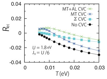
Figure 17: Temperature dependence of $R_{\textrm{H}}$ at $U=1.8$ eV and $J_{\textrm{H}}=\frac{U}{6}$ in the four cases.

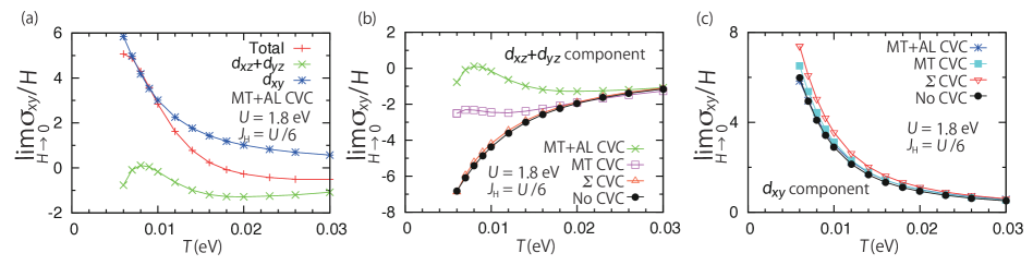
Figure 18: Temperature dependence of $\textstyle\lim_{H\rightarrow 0}\frac{\sigma_{xy}}{H}$ and orbital-decomposed components in the MT$+$AL CVC case at $U=1.8$ eV and the orbital-decomposed components of (b) the $d_{xz}$ and $d_{yz}$ orbitals and (c) $d_{xy}$ orbital in the four cases at $U=1.8$ eV.

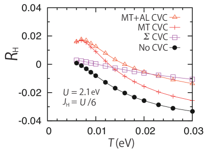
Figure 19: Temperature dependence of $R_{\textrm{H}}$ at $U=2.1$ eV and $J_{\textrm{H}}=\frac{U}{6}$ in the four cases.

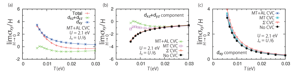
Figure 20: Temperature dependence of $\textstyle\lim_{H\rightarrow 0}\frac{\sigma_{xy}}{H}$ and the orbital-decomposed components in the MT$+$AL CVC case at $U=2.1$ eV and the orbital-decomposed components of (b) the $d_{xz}$ and $d_{yz}$ orbitals and (c) $d_{xy}$ orbital in the four cases at $U=2.1$ eV.

We start discussing $R_{\textrm{H}}(=\sigma_{xx}^{-2}\textstyle\lim_{H\rightarrow 0}\frac{\sigma_{xy}}{H})$ away from the AF QCP. We show its temperature dependence in the four cases in Fig. 17, and see from that figure three main features in the MT$+$AL CVC case. First, at high temperatures, the values of $R_{\textrm{H}}$ in the MT$+$AL CVC case are close to the values in the $\Sigma$ CVC case. This origin is the same for $\rho_{ab}$ at high temperatures, i.e., the small effects of the MT and the AL CVCs due to the large QP damping. Second, when temperature is low, the value of $R_{\textrm{H}}$ in the MT$+$AL CVC case becomes almost the same as that in the MT CVC case. This result can be understood that the main effects of the MT CVC on $R_{\textrm{H}}$ at low temperatures remain leading even including the main terms of the AL CVC. Its mechanism is as follows: As shown in Ref. NA-CVC, , the main effects of the MT CVC on $R_{\textrm{H}}$ at low temperatures are the decreases of the negative-sign contributions of the $d_{xz}+d_{yz}$ component of the transverse conductivity around $\bm{k}=(\frac{21}{32}\pi,\frac{21}{32}\pi)$ as a result of the magnitude changes of the currents of the $d_{xz/yz}$ orbital around $\bm{k}=(\frac{21}{32}\pi,\frac{21}{32}\pi)$ due to the MT CVC arising from the spin fluctuations of the $d_{xz/yz}$ orbital around $\bm{q}=\bm{Q}_{\textrm{IC-AF}}$. Although the currents of the $d_{xz/yz}$ orbital around $\bm{k}=(\frac{21}{32}\pi,\frac{21}{32}\pi)$ are affected by the AL1 and AL2 CVCs arising from the above spin fluctuations, the main effects of the MT CVC persist in the MT$+$AL CVC case due to the cancellation of those AL1 and AL2 CVCs in the presence of the even-parity and the rotational symmetry. (The mechanism of this cancellation Kon-CVC was explained in Sect. III C 1.) It should be noted that we can understand why only for $R_{\textrm{H}}$ the main effects of the MT CVC survive at low temperatures even with the main terms of the AL CVC by considering the difference between the important factors for $\sigma_{xx}$ and $\textstyle\lim_{H\rightarrow 0}\frac{\sigma_{xy}}{H}$: since the important factor for $\sigma_{xx}$ is the unrenormalized QP damping, the effects of the MT CVC on the currents of the $d_{xz/yz}$ orbital around $\bm{k}=(\frac{21}{32}\pi,\frac{21}{32}\pi)$ are little important for $\rho_{ab}$ away from the AF QCP due to the large unrenormalized QP damping; on the other hand, since not only the unrenormalized QP damping but also the momentum derivative of the angle of the current becomes important for $\textstyle\lim_{H\rightarrow 0}\frac{\sigma_{xy}}{H}$, the effects of the MT CVC on the currents of the $d_{xz/yz}$ orbital around $\bm{k}=(\frac{21}{32}\pi,\frac{21}{32}\pi)$ become considerable for $R_{\textrm{H}}$ due to the large momentum derivative. Third, three specific features of $R_{\textrm{H}}$ obtained in the MT CVC case survive even including the main terms of the AL CVC; the three specific features are emerging a peak, crossing over zero, and increasing monotonically in the high-temperature region. This can be understood that at high temperatures the effects of the AL CVC are small due to the large QP damping, and that the main effects of the MT CVC at low temperatures remain qualitatively unchanged.

Next, we analyze the orbital-decomposed components of $\lim\limits_{H\rightarrow 0}\frac{\sigma_{xy}}{H}$ away from the AF QCP to determine the role of each $t_{2g}$ orbital. Due to the same reason for $\sigma_{xx}$, we consider only the $d_{xz}+d_{yz}$ component and $d_{xy}$ component of $\textstyle\lim_{H\rightarrow 0}\frac{\sigma_{xy}}{H}$; the former and the latter are defined as the equations that $\textstyle\sum_{\{a\}=1}^{3}$ in Eq. (39) are replaced by, respectively, $\textstyle\sum_{\{a\}=1}^{2}$ and $\textstyle\sum_{\{a\}=3}$. From Figs. 18(a)–18(c), we find three main properties: at high temperatures, the effects of all the CVCs on those components are very small; in the low-temperature region, the temperature dependence in the MT$+$AL CVC case is qualitatively the same for the MT CVC case; a peak of the $d_{xz}+d_{yz}$ component survives even with the main terms of the AL CVC. Those results can be understood in the similar way for $R_{\textrm{H}}$. It should be noted that the difference in the important factor is the origin why the $d_{xy}$ orbital gives considerable contributions to only $\textstyle\lim_{H\rightarrow 0}\frac{\sigma_{xy}}{H}$, although its contributions to $\sigma_{xx}$ are negligible.

Thus, we deduce from the results at $U=1.8$ eV that the qualitative behavior of $R_{\textrm{H}}$ away from the AF QCP can be captured by taking account of the $\Sigma$ CVC and the MT CVC.

Then, we go on to analyze the temperature dependence of $R_{\textrm{H}}$ near the AF QCP. The results at $U=2.1$ eV in the four cases are shown in Fig. 19. We see that even including the main terms of the AL CVC, $R_{\textrm{H}}$ shows three specific features (emerging a peak, crossing over zero, and increasing monotonically in high-temperature region), and that $R_{\textrm{H}}$ has two almost distinct regions as a function of temperature. The former result can be understood in the same way as the explanations about the third result of $R_{\textrm{H}}$ away from the AF QCP, and the latter can be understood in the same way for the similar property of $\rho_{ab}$ near the AF QCP (see Sect. III C 1).

Moreover, we determine the orbital dependence of $\textstyle\lim_{H\rightarrow 0}\frac{\sigma_{xy}}{H}$ near the AF QCP by the analyses of the temperature dependence of the $d_{xz}+d_{yz}$ component and $d_{xy}$ component. From Figs. 20(a)–20(c), we see three features the same as those obtained away from the AF QCP. Furthermore, comparing the results away from and near the AF QCP, we find that the difference in the $d_{xz}+d_{yz}$ component or $d_{xy}$ component between the MT CVC case and the MT$+$AL CVC case becomes smaller near the AF QCP than away from the AF QCP. This results from the more importance of the MT CVC near the AF QCP.

Thus, the results at $U=2.1$ eV show the validity of the qualitative behaviors of $R_{\textrm{H}}$ near the AF QCP in the MT CVC case and the existence of the two almost distinct regions of the temperature dependence of $R_{\textrm{H}}$ near the AF QCP, which are the same for $\rho_{ab}$ near the AF QCP.

IV Discussions

In this section, I compare the results obtained away from or near the AF QCP with several experimental or theoretical results. The discussions in Sec. IV A are for the comparisons with several experiments, and the discussions in Sec. IV B are for the comparisons with other theories.

IV.1 Comparisons with experiments

In this section, we compare the results obtained away from or near the AF QCP with several experiments of Sr₂RuO₄ or Sr₂Ru_0.975Ti_0.025O₄, respectively, and see that the obtained results are qualitatively consistent with these experiments. In the comparisons with Sr₂Ru_0.975Ti_0.025O₄, I believe that the physical origins of several behaviors observed experimentally can be deduced by comparison with the results obtained near the AF QCP. This is because the main effect of the Ti-substitution may be the system approaching towards the AF QCP compared with Sr₂RuO₄; this main effect can be treated by increasing the value of $U$ in the model of Sr₂RuO₄. Although the microscopic mechanism why the Ti-substitution causes approaching towards the AF QCP is unclear, we can qualitatively understand several differences between Sr₂RuO₄ and Sr₂Ru_0.975Ti_0.025O₄ as a result of the difference in the distance from the AF QCP, as I will show below.

We begin with the comparisons about the magnetic properties. The enhancement of the spin susceptibility at $\bm{q}=\bm{Q}_{\textrm{IC-AF}}$ away from the AF QCP agrees with the neutron Neutron-x2 or the nuclear-magnetic-resonance (NMR) Ishida-NMR-x2 measurement of Sr₂RuO₄, and the similar enhancement near the AF QCP is consistent with the neutron Neutron-Ti214 or the NMR Ishida-NMR-x05 measurement of Sr₂Ru_0.975Ti_0.025O₄. Also, no sizable commensurate ferromagnetic spin fluctuation obtained away from the AF QCP is in agreement with the neutron measurement Neutron-x2 of Sr₂RuO₄. Thus, several magnetic properties can be well described in the FLEX approximation, as explained in Ref. NA-CVC, . It should be noted that to discuss the anisotropy between the inplane and the out-of-plane spin susceptibilities, the spin-orbit interaction is necessary Yanase-Ru .

Then, we turn to the comparisons about the electronic structure. As discussed in Ref. NA-CVC, , the larger mass enhancement for the $d_{xy}$ orbital than for the $d_{xz/yz}$ orbital away from the AF QCP is consistent with an experiment dHvA-x2 ; Mackenzie-review in Sr₂RuO₄. In addition, the topology of the FS away from the AF QCP agrees with the measurement of the dHvA effect dHvA-x2 or the angle-resolved photoemission spectroscopy ARPES-x2 . However, there is a quantitative difference in the location of the FS sheet of the $d_{xy}$ orbital near $\bm{k}=(\frac{2}{3}\pi,\frac{2}{3}\pi)$: in my result, that FS sheet is very close to the inner FS sheet of the $d_{xz/yz}$ orbital [see Fig. 9(a)]; in the experiments dHvA-x2 ; ARPES-x2 , that FS sheet is not very close to the inner FS sheet. That difference exists even in the LDA Oguchi ; Mazin-LDA , as described in Ref. NA-CVC, . To improve that difference, the spin-orbit interaction of the Ru ions will be necessary since the small spin-orbit interaction leads to the weak hybridization of the bands near $\bm{k}=(\frac{2}{3}\pi,\frac{2}{3}\pi)$ Oguchi-LS . Actually, that difference is improved in the local-spin-density approximation Oguchi-LS including the spin-orbit interaction. Although that result indicates the importance of the spin-orbit interaction for quantitative discussions, the qualitative agreement of the FS is meaningful since that qualitative agreement suggests that the present theory can capture the aspects of many-body effects on the FS of Sr₂RuO₄ at least on a qualitative level. In addition, that qualitative agreement supports the suitability of the expectation that the electronic structure of Sr₂RuO₄ in the LDA Oguchi ; Mazin-LDA may be regarded as a good starting point to include many-body effects. This is another meaningful aspect of that qualitative agreement since electron correlation sometimes modifies the FS drastically, resulting in the deviation of the FS from the experiment even on a qualitative level Ikeda-FLEX . From those comparisons, we deduce that the FLEX approximation can qualitatively well describe the electronic structure of Sr₂RuO₄.

Finally, I compare the obtained results with the experimental results about the transport properties. As described in Ref. NA-CVC, , the $T^{2}$ dependence of $\rho_{ab}$ at low temperatures and the non-monotonic temperature dependence of $R_{\textrm{H}}$ away from the AF QCP are qualitatively consistent with the experiments resistivity-x2 ; Hall-x2 of $\rho_{ab}$ and $R_{\textrm{H}}$ of Sr₂RuO₄, and the $T$-linear $\rho_{ab}$ near the AF QCP can qualitatively explain the experimental result Ti214-nFL2 in Sr₂Ru_0.975Ti_0.025O₄. (The detail of the temperature dependence of $R_{\textrm{H}}$ in Sr₂RuO₄ was described in Sec. I.) Although the spin-orbit interaction generally leads to an additional contribution to $R_{\textrm{H}}$ through the anomalous Hall effect Kon-AHE , it has been experimentally confirmed that such contribution is small CSRO-nFL2 . Thus, neglecting the spin-orbit interaction will be sufficient for at least qualitative discussions about $R_{\textrm{H}}$. Combining those discussions, we find that the successful descriptions of the transport properties qualitatively hold in the FLEX approximation with the $\Sigma$ CVC, the MT CVC, and the main terms of the AL CVC.

IV.2 Comparisons with other theories

In this section, we compare the results of this paper with other theoretical studies and show several better points of this theory. First, we focus on the comparisons with the DMFT Haule-DMFT ; Georges-DMFT-Ru for a model of Sr₂RuO₄, and show that several electronic properties can be better described in the method I used due to a sufficient treatment of the spatially modulated spin fluctuations. Then, we compare my results with the transport properties of Sr₂RuO₄ obtained in the phenomenological Boltzmann theory within the relaxation-time approximation Hall-theory-x2 , and point out the importance of the MT CVC arising from the spin fluctuations of the $d_{xz/yz}$ orbital in order to naturally obtain the non-monotonic temperature dependence of $R_{\textrm{H}}$ without any ad hoc parameters of the unrenormalized QP damping. Finally, we discuss the similarities and differences between the main effects of the AL CVC on the charge transports in my case and the case Kon-CVC of the single-orbital Hubbard model near an AF QCP on a square lattice, and conclude that the existence of the two almost distinct regions of the charge transports near an AF QCP as a function of temperature is one of the important findings of this paper.

We begin with the comparisons about the magnetic properties, the orbital dependence of the mass enhancement, and the modification of the FS sheets due to electron correlation in the DMFT Haule-DMFT ; Georges-DMFT-Ru for a model of Sr₂RuO₄ in more detail than Ref. NA-CVC, . First, in the DMFT, spatial correlations, the momentum dependent fluctuations, are completely neglected Metzner , and the effects of only local correlations are taken into account Georges-review ; Kotliar-review . On the other hand, I have shown that not local but spatially modulated spin fluctuation with $\bm{q}=\bm{Q}_{\textrm{IC-AF}}$ is important to discuss the magnetic properties of Sr₂RuO₄. As explained in Sect. IV A, the neutron Neutron-x2 and the NMR Ishida-NMR-x2 measurement for Sr₂RuO₄ have observed the enhancement of that spatially modulated spin fluctuation. Thus, the magnetic properties can be better described in my case. Second, in the DMFT, the locations of the FS sheets are more drastically modified due to electron correlation than in my case: on $k_{x}=k_{y}$ line, the $\gamma$ sheet of the $d_{xy}$ orbital becomes the most inner sheet in the DMFT Georges-DMFT-Ru , while the most inner sheet in the LDA Oguchi ; Mazin-LDA or my case is the $\beta$ sheet of the $d_{xz/yz}$ orbital. Since the experimental results dHvA-x2 ; ARPES-x2 are consistent with the result in the LDA Oguchi ; Mazin-LDA and my case, the agreement about the FS is better in my case than in the DMFT Georges-DMFT-Ru . Third, in the DMFT, the mass enhancement of the $d_{xy}$ orbital is larger than that of the $d_{xz/yz}$ orbital for finite values of $J_{\textrm{H}}$ Haule-DMFT ; e.g., the former and the latter become $3.2$ and $2.4$ at $U=2.3$ eV and $J_{\textrm{H}}=0.3$ eV ($\sim 0.13U$) or $4.5$ and $3.3$ at $U=2.3$ eV and $J_{\textrm{H}}=0.4$ eV ($\sim 0.174U$). Thus, the larger mass enhancement for the $d_{xy}$ orbital than for the $d_{xz/yz}$ orbital is obtained in both the DMFT Haule-DMFT and the FLEX approximation, although the large mass enhancement of the $d_{xy}$ orbital is realized in a wider region of the parameters space in my case than in the DMFT Haule-DMFT ; in particular, that larger mass enhancement of the $d_{xy}$ orbital is obtained even at $J_{\textrm{H}}=0$ eV in my case NA-CVC . It should be noted that it is important and necessary to check whether spatial correlations, neglected in the DMFT Metzner , keep the orbital dependence of the mass enhancement qualitatively the same since the spatial correlations sometimes drastically change the results obtained in the DMFT (e.g., see case cDMFT-Kotliar of a single-orbital Hubbard model on a square lattice). Actually, even in a two-orbital Hubbard model cDMFT-Arita on a square lattice, spatial correlations included by considering a cluster cause the almost perfect disappearance of the unusual $J_{\textrm{H}}$ dependence of a critical value of $U$ for a Mott transition, which is obtained in the DMFT. Combining the discussions of this paragraph, I conclude that several electronic properties of Sr₂RuO₄ can be better described in my case than in the DMFT Haule-DMFT ; Georges-DMFT-Ru . In particular, it is significant to find the importance of the MT CVC for obtaining the non-monotonic temperature dependence of $R_{\textrm{H}}$ of Sr₂RuO₄ in this paper since in the DMFT the CVCs are neglected due to lack of the momentum dependence of the self-energy DMFT-CVC1 ; DMFT-CVC2 .

I turn to the comparisons about the transport properties of Sr₂RuO₄ with the phenomenological Boltzmann theory in the relaxation-time approximation Hall-theory-x2 , in which all the CVCs are neglected Kon-review . In the relaxation-time approximation for Sr₂RuO₄, the unrenormalized QP damping, $\tau_{a}^{-1}$, is given by $\tau_{a}^{-1}=\eta_{a}+\alpha_{a}T^{2}$ with the ad-hoc parameters $\eta_{a}$ and $\alpha_{a}$, which are chosen as $\eta_{d_{xz}}=\eta_{d_{yz}}=2.75$, $\eta_{d_{xy}}=3.25$, $\alpha_{d_{xz}}=0.035$, $\alpha_{d_{yz}}=0.04$, and $\alpha_{d_{xy}}=0.06$; this form of $\tau_{a}^{-1}$ as a function of temperature is typical of the FL AGD ; NA-review ; Morel-Nozieres . In addition, only for the calculation of the in-plane resistivity, the authors of Ref. Hall-theory-x2, added $0.6T$ to $\tau_{d_{xy}}^{-1}$ since they assumed that Sr₂RuO₄ were close to a ferromagnetic instability. Although that assumption is experimentally incorrect Neutron-x2 ; Ishida-NMR-x2 , their results at low temperatures will remain qualitatively unchanged since the contribution from the $d_{xz/yz}$ orbital is more important than that from the $d_{xy}$ orbital due to the smaller $\tau_{a}^{-1}$ of the $d_{xz/yz}$ orbital. Adopting the phenomenological Boltzmann theory in the relaxation-time approximation with those expressions of the unrenormalized QP damping to $\rho_{ab}$ and $R_{\textrm{H}}$, the authors of Ref. Hall-theory-x2, obtained the $T^{2}$ dependence of $\rho_{ab}$ at low temperatures and the non-monotonic temperature dependence of $R_{\textrm{H}}$, which are consistent with the experiments resistivity-x2 ; Hall-x2 . However, as they pointed out in Ref. Hall-theory-x2, , the result of $R_{\textrm{H}}$ is very sensitive to the small relative variation of $\alpha_{d_{xz}}$ and $\alpha_{d_{yz}}$, and the sign change of $R_{\textrm{H}}$ disappears in some cases. In addition, $\alpha_{d_{xz}}$ and $\alpha_{d_{yz}}$ should be the same due to the tetragonal symmetry of the crystal. Thus, although the results obtained in the relaxation-time approximation Hall-theory-x2 seem to be reasonable, the validity of the choice of the ad hoc parameters is unclear. On the other hand, I have shown in Ref. NA-CVC, without any ad hoc parameters of the unrenormalized QP damping that the MT CVC arising from the spin fluctuations of the $d_{xz/yz}$ orbital is essential to obtain the non-monotonic temperature dependence of $R_{\textrm{H}}$. Furthermore, in this paper, I show that the importance of that MT CVC remains unchanged even if we consider the main terms of the AL CVC. From those arguments, I propose the importance of the MT CVC arising from the spin fluctuations of the $d_{xz/yz}$ orbital to understand the temperature dependence of $R_{\textrm{H}}$ of Sr₂RuO₄.

I close this section with the comparisons about the main effects of the AL CVC with the case Kon-CVC of the single-orbital Hubbard model near an AF QCP on a square lattice. In that single-orbital case, the authors of Ref. Kon-CVC, analytically or numerically studied the effects of the AL CVC on $\rho_{ab}$ and $R_{\textrm{H}}$ near the AF QCP where the spin susceptibility at $\bm{q}=(\pi,\pi)$ was most strongly enhanced. Then, their analytic study revealed the cancellation of the leading contributions in the AL$1$ or the AL$2$ CVC near the AF QCP, whose details were explained in Sect. III C 1, and their numerical study considering only the contributions of the MT CVC and the AL CVC from the states on the Fermi level revealed the qualitative validity of the results obtained without the AL CVC. However, due to neglecting the other contributions near the Fermi level, they did not obtain the existence of the two almost distinct regions of the transport properties near the AF QCP as a function of temperature, which is revealed in this paper. It should be noted that I obtained the similar results Kon-CVC to those they had obtained, a decrease of the value of the inplane resistivity due to the AL CVC and a larger decrease of that at high temperatures than at low temperatures (see Fig. 15). Thus, the aspects of the AL CVC in my case are qualitatively consistent with those in the single-orbital case Kon-CVC . In addition, it is one of the important findings of this paper to reveal the existence of the two almost distinct regions of the charge transports near an AF QCP.

V Summary

In summary, after explaining the formal derivations of $\rho_{ab}$, $R_{\textrm{H}}$, and the FLEX approximation with the $\Sigma$ CVC, the MT CVC, and the AL CVC, I studied $\rho_{ab}$ and $R_{\textrm{H}}$ for a $t_{2g}$-orbital Hubbard model in a PM state near or away from the AF QCP on a square lattice in the FLEX approximation with the $\Sigma$ CVC, the MT CVC, and the main terms of the AL CVC, and then found the three main results about many-body effects. The first main result is showing that the results of the previous studies NA-CVC ; NA-review remain qualitatively unchanged even with the main terms of the AL CVC. This indicates the qualitative validity of the arguments in the previous studies NA-CVC ; NA-review . The second main result is finding the two almost distinct regions of the charge transports near the AF QCP: $\rho_{ab}$ and $R_{\textrm{H}}$ in the high-temperature region are described by including only the $\Sigma$ CVC, while the $\Sigma$ CVC and the MT CVC are necessary for their descriptions in low-temperature region. The third main result is clarifying the difference of the effects of the MT CVC between $\rho_{ab}$ and $R_{\textrm{H}}$ away from the AF QCP at low temperatures: the MT CVC leads to the considerable effect only on the latter, although at high temperatures only the $\Sigma$ CVC affects $\rho_{ab}$ and $R_{\textrm{H}}$. Thus, the second and third main results highlight the important aspects of many-body effects on the charge transports. I also showed several results of the magnetic properties and the electronic structure for that model in the FLEX approximation. Those support a deeper understanding than in the previous studies NA-CVC ; NA-review . Then, comparing the obtained results with several experiments, I achieved the qualitative agreement about the momentum dependence of the spin fluctuation in Sr₂RuO₄ Neutron-x2 ; Ishida-NMR-x2 or Sr₂Ru_0.975Ti_0.025O₄ Neutron-Ti214 ; Ishida-NMR-x05 , the orbital dependence of the mass enhancement in Sr₂RuO₄ dHvA-x2 ; Mackenzie-review , the topology of the FS of Sr₂RuO₄ dHvA-x2 ; ARPES-x2 , the $T^{2}$ dependence resistivity-x2 of $\rho_{ab}$ at low temperatures in Sr₂RuO₄, the non-monotonic temperature dependence Hall-x2 of $R_{\textrm{H}}$ in Sr₂RuO₄, and the $T$-linear $\rho_{ab}$ in Sr₂Ru_0.975Ti_0.025O₄ Ti214-nFL2 . Furthermore, by the comparisons with other theories, I showed several stronger points to discuss the electronic properties of Sr₂RuO₄ than other theories Haule-DMFT ; Georges-DMFT-Ru ; Hall-theory-x2 , and clarified the similarities and differences of the main effects of the AL CVC between the present multiorbital case and a single-orbital case Kon-CVC .

Several important issues remain for further study. One is the extension of the present method to case with the spin-orbit interaction. In particular, it is desirable to study the anisotropy between the inplane and the out-of-plane susceptibility, the quantitative effects on the FS deformation including many-body effects, and the charge Hall effect including both the usual Hall effect and the anomalous Hall effect. It is also important to extend the present method to case CSRO-nFL1 ; CSRO-nFL2 with the RuO₆ distortions near the ferromagnetic QCP since its results and the present results lead to deep understanding of the similarities and differences between many-body effects on the charge transports near the ferromagnetic and the AF QCPs. Furthermore, the study about the charge transports of the $3$D ruthenates Ru113 using the extended method is useful to clarify the role of the dimensionality in the charge transports of a correlated multiorbital system. Then, another important issue is the extended study about the charge or heat transports of Sr₂RuO₄ in a superconducting phase SC-trans1 ; SC-trans2 since it may clarify the role of each $t_{2g}$ orbital in the superconducting phase. Finally, it is challenging and important to study the charge transports of other transition-metal oxides MIT-review or the heavy-fermion materials such as CeCoIn₅ Ce115 and UPt₃ UPt3 or the organic conductors organic-review by extending the present method and adopting that to other multiorbital Hubbard models or the multiorbital Anderson models. Their achievements may provide deeper knowledge about ubiquitous or characteristic properties of many-body effects on the charge transports of a correlated multiorbital system.

Appendix A Derivation of Eq. (13)

In this appendix, we derive Eq. (13) from Eq. (10). In this derivation, we use the analytic properties of the single-particle Green’s function and reducible four-point vertex function in terms of frequency variables. The former becomes singular for $\textrm{Im}\epsilon=0$ with $\epsilon$ being its frequency variable. The analytic property of the latter is the same for the two-particle Green’s function Eliashberg-theory : it becomes singular when the frequency variables $\epsilon$, $\epsilon^{\prime}$, and $\omega$ satisfy $\textrm{Im}\epsilon=0$ or $(\textrm{Im}\epsilon+\textrm{Im}\omega)=0$ or $\textrm{Im}\epsilon^{\prime}=0$ or $(\textrm{Im}\epsilon^{\prime}+\textrm{Im}\omega)=0$ or $(\textrm{Im}\epsilon+\textrm{Im}\epsilon^{\prime}+\textrm{Im}\omega)=0$ or $(\textrm{Im}\epsilon-\textrm{Im}\epsilon^{\prime})=0$, where we consider case for $\textrm{Im}\omega>0$ to take $i\Omega_{n}\rightarrow\omega+i0+$. As a result, there are $16$ possibilities of the four-point vertex function in real-frequency representation, as shown in Table 1.

Table 1: Relation between the additional subscripts of the four-point vertex function and the inequalities of its frequency variables. Because of $\textrm{Im}\omega>0$ and the analytic properties of the four-point vertex function, there are $16$ possibilities.

region	$\textrm{Im}\epsilon$	$\textrm{Im}\epsilon+\textrm{Im}\omega$	$\textrm{Im}\epsilon^{\prime}$	$\textrm{Im}\epsilon^{\prime}+\textrm{Im}\omega$	$\textrm{Im}\epsilon+\textrm{Im}\epsilon^{\prime}+\textrm{Im}\omega$	$\textrm{Im}\epsilon-\textrm{Im}\epsilon^{\prime}$
11-I	$>0$	$>0$	$>0$	$>0$	$>0$	$>0$
11-II	$>0$	$>0$	$>0$	$>0$	$>0$	$<0$
21	$<0$	$>0$	$>0$	$>0$	$>0$	$<0$
31-II	$<0$	$<0$	$>0$	$>0$	$>0$	$<0$
31-I	$<0$	$<0$	$>0$	$>0$	$<0$	$<0$
32	$<0$	$<0$	$<0$	$>0$	$<0$	$<0$
33-I	$<0$	$<0$	$<0$	$<0$	$<0$	$<0$
33-II	$<0$	$<0$	$<0$	$<0$	$<0$	$>0$
23	$<0$	$>0$	$<0$	$<0$	$<0$	$>0$
13-II	$>0$	$>0$	$<0$	$<0$	$<0$	$>0$
13-I	$>0$	$>0$	$<0$	$<0$	$>0$	$>0$
12	$>0$	$>0$	$<0$	$>0$	$>0$	$>0$
22-III	$<0$	$>0$	$<0$	$>0$	$>0$	$>0$
22-II	$<0$	$>0$	$<0$	$>0$	$>0$	$<0$
22-I	$<0$	$>0$	$<0$	$>0$	$<0$	$<0$
22-IV	$<0$	$>0$	$<0$	$>0$	$<0$	$>0$

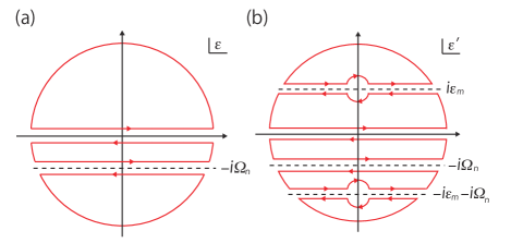
Figure 21: Contours used for the analytic continuations of Eq. (10). Contour shown in panel (b) is one of the possibilities.

Using those analytic properties, we can carry out the analytic continuations of the first and the second terms of Eq. (10). This is because we can rewrite the summation about the Matsubara frequency as the corresponding contour integral AGD . Using the contour $C$ shown in Fig. 21(a), we can carry out the analytic continuation for the first term:

$$-\frac{T}{N}\sum\limits_{\bm{k}}\sum\limits_{m}\sum\limits_{\{a\}}(v_{\bm{k}\nu})_{ba}(v_{\bm{k}\nu})_{cd}G_{ac}(\bm{k},i\epsilon_{m+n})G_{db}(\bm{k},i\epsilon_{m})$$

$$=-\frac{1}{N}\sum\limits_{\bm{k}}\int_{\textrm{C}}\frac{d\epsilon}{4\pi i}\tanh\frac{\epsilon}{2T}\sum\limits_{\{a\}}(v_{\bm{k}\nu})_{ba}(v_{\bm{k}\nu})_{cd}$$

$$\times G_{ac}(\bm{k},\epsilon+i\Omega_{n})G_{db}(\bm{k},\epsilon)$$

$$\rightarrow-\frac{1}{N}\sum\limits_{\bm{k}}\int_{-\infty}^{\infty}\frac{d\epsilon}{4\pi i}\sum\limits_{\{a\}}(v_{\bm{k}\nu})_{ba}(v_{\bm{k}\nu})_{cd}$$

$$\times\Bigl{[}\tanh\frac{\epsilon}{2T}g_{1;acdb}(k;\omega)$$

$$+\Bigl{(}\tanh\dfrac{\epsilon+\omega}{2T}-\tanh\dfrac{\epsilon}{2T}\Bigr{)}g_{2;acdb}(k;\omega)$$

$$-\tanh\dfrac{\epsilon+\omega}{2T}g_{3;acdb}(k;\omega)\Bigr{]},$$ (80)

where $\rightarrow$ represents the replacement of $i\Omega_{n}$ by $\omega+i0+$, and $g_{l;acdb}(k;\omega)$ are

$$g_{1;acdb}(k;\omega)= \ G_{ac}^{(\textrm{R})}(\bm{k},\epsilon+\omega)G_{db}^{(\textrm{R})}(\bm{k},\epsilon),$$ (81)

$$g_{2;acdb}(k;\omega)= \ G_{ac}^{(\textrm{R})}(\bm{k},\epsilon+\omega)G_{db}^{(\textrm{A})}(\bm{k},\epsilon),$$ (82)

and

$$g_{3;acdb}(k;\omega)= \ G_{ac}^{(\textrm{A})}(\bm{k},\epsilon+\omega)G_{db}^{(\textrm{A})}(\bm{k},\epsilon).$$ (83)

Next, by replacing $T\sum_{m}$ and $T\sum_{m^{\prime}}$ in the second term of Eq. (10) by the contour integrals with the contour $C$ in Fig. 21(a) and the contour $C^{\prime}$ such as Fig. 21(b), respectively, we can similarly carry out the analytic continuation of the second term:

$$-\frac{T^{2}}{N^{2}}\sum\limits_{\bm{k},\bm{k}^{\prime}}\sum\limits_{m,m^{\prime}}\sum\limits_{\{a\}}\sum\limits_{\{A\}}(v_{\bm{k}\nu})_{ba}(v_{\bm{k}^{\prime}\nu})_{cd}G_{aA}(\bm{k},i\epsilon_{m+n})G_{dD}(\bm{k}^{\prime},i\epsilon_{m^{\prime}})\Gamma_{\{A\}}(\bm{k},i\epsilon_{m},\bm{k}^{\prime},i\epsilon_{m^{\prime}};\bm{0},i\Omega_{n})$$

$$\ \ \ \times G_{Bb}(\bm{k},i\epsilon_{m})G_{Cc}(\bm{k}^{\prime},i\epsilon_{m^{\prime}+n})$$

$$= -\frac{1}{N^{2}}\sum\limits_{\bm{k},\bm{k}^{\prime}}\int_{\textrm{C}}\frac{d\epsilon}{4\pi i}\tanh\frac{\epsilon}{2T}\sum\limits_{\{a\}}\sum\limits_{\{A\}}(v_{\bm{k}\nu})_{ba}(v_{\bm{k}^{\prime}\nu})_{cd}G_{aA}(\bm{k},\epsilon+i\Omega_{n})G_{Bb}(\bm{k},\epsilon)$$

$$\ \times\Bigl{[}\int_{\textrm{C}^{\prime}}\frac{d\epsilon^{\prime}}{4\pi i}\tanh\frac{\epsilon^{\prime}}{2T}G_{dD}(\bm{k}^{\prime},\epsilon^{\prime})\Gamma_{\{A\}}(\bm{k},\epsilon,\bm{k}^{\prime},\epsilon^{\prime};\bm{0},i\Omega_{n})G_{Cc}(\bm{k}^{\prime},\epsilon^{\prime}+i\Omega_{n})$$

$$\ \ \ \ +TG_{dD}(\bm{k}^{\prime},\epsilon)\Gamma_{\{A\}}(\bm{k},\epsilon,\bm{k}^{\prime},\epsilon;\bm{0},i\Omega_{n})G_{Cc}(\bm{k}^{\prime},\epsilon+i\Omega_{n})$$

$$\ \ \ \ +TG_{dD}(\bm{k}^{\prime},-\epsilon-i\Omega_{n})\Gamma_{\{A\}}(\bm{k},\epsilon,\bm{k}^{\prime},-\epsilon-i\Omega_{n};\bm{0},i\Omega_{n})G_{Cc}(\bm{k}^{\prime},-\epsilon)\Bigr{]}$$

$$\rightarrow -\frac{1}{N^{2}}\sum\limits_{\bm{k},\bm{k}^{\prime}}\sum\limits_{\{a\}}(v_{\bm{k}\nu})_{ba}(v_{\bm{k}^{\prime}\nu})_{cd}\sum\limits_{\{A\}}\int^{\infty}_{-\infty}\frac{d\epsilon}{4\pi i}\int^{\infty}_{-\infty}\frac{d\epsilon^{\prime}}{4\pi i}\coth\dfrac{\epsilon^{\prime}-\epsilon}{2T}$$

$$\times\Bigl{\{}\Bigl{(}\tanh\dfrac{\epsilon+\omega}{2T}-\tanh\dfrac{\epsilon}{2T}\Bigr{)}g_{2;aABb}(k;\omega)g_{2;CcdD}(k^{\prime};\omega)\Bigl{[}\Gamma_{22\textrm{-II};\{A\}}(k,k^{\prime};\omega)-\Gamma_{22\textrm{-III};\{A\}}(k,k^{\prime};\omega)\Bigr{]}$$

$$-\tanh\dfrac{\epsilon+\omega}{2T}g_{3;aABb}(k;\omega)g_{3;CcdD}(k^{\prime};\omega)\Bigl{[}\Gamma_{33\textrm{-I};\{A\}}(k,k^{\prime};\omega)-\Gamma_{33\textrm{-II};\{A\}}(k,k^{\prime};\omega)\Bigr{]}$$

$$+\tanh\dfrac{\epsilon}{2T}g_{1;aABb}(k;\omega)g_{1;CcdD}(k^{\prime};\omega)\Bigl{[}\Gamma_{11\textrm{-II};\{A\}}(k,k^{\prime};\omega)-\Gamma_{11\textrm{-I};\{A\}}(k,k^{\prime};\omega)\Bigr{]}\Bigr{\}}$$

$$-\frac{1}{N^{2}}\sum\limits_{\bm{k},\bm{k}^{\prime}}\sum\limits_{\{a\}}(v_{\bm{k}\nu})_{ba}(v_{\bm{k}^{\prime}\nu})_{cd}\sum\limits_{\{A\}}\int^{\infty}_{-\infty}\dfrac{d\epsilon}{4\pi i}\int^{\infty}_{-\infty}\dfrac{d\epsilon^{\prime}}{4\pi i}\tanh\dfrac{\epsilon^{\prime}}{2T}$$

$$\times\Bigl{\{}\Bigl{(}\tanh\dfrac{\epsilon+\omega}{2T}-\tanh\dfrac{\epsilon}{2T}\Bigr{)}g_{2;aABb}(k;\omega)\Bigl{[}\Gamma_{21;\{A\}}(k,k^{\prime};\omega)g_{1;CcdD}(k^{\prime};\omega)-\Gamma_{22\textrm{-II};\{A\}}(k,k^{\prime};\omega)g_{2;CcdD}(k^{\prime};\omega)\Bigr{]}$$

$$-\tanh\dfrac{\epsilon+\omega}{2T}g_{3;aABb}(k;\omega)\Bigl{[}\Gamma_{31\textrm{-I};\{A\}}(k,k^{\prime};\omega)g_{1;CcdD}(k^{\prime};\omega)-\Gamma_{32;\{A\}}(k,k^{\prime};\omega)g_{2;CcdD}(k^{\prime};\omega)\Bigr{]}$$

$$+\tanh\frac{\epsilon}{2T}g_{1;aABb}(k;\omega)\Bigl{[}\Gamma_{11\textrm{-I};\{A\}}(k,k^{\prime};\omega)g_{1;CcdD}(k^{\prime};\omega)-\Gamma_{12;\{A\}}(k,k^{\prime};\omega)g_{2;CcdD}(k^{\prime};\omega)\Bigr{]}\Bigr{\}}$$

$$-\dfrac{1}{N^{2}}\sum\limits_{\bm{k},\bm{k}^{\prime}}\sum\limits_{\{a\}}(v_{\bm{k}\nu})_{ba}(v_{\bm{k}^{\prime}\nu})_{cd}\sum\limits_{\{A\}}\int^{\infty}_{-\infty}\dfrac{d\epsilon}{4\pi i}\int^{\infty}_{-\infty}\dfrac{d\epsilon^{\prime}}{4\pi i}\tanh\dfrac{\epsilon^{\prime}+\omega}{2T}$$

$$\times\Bigl{\{}\Bigl{(}\tanh\dfrac{\epsilon+\omega}{2T}-\tanh\dfrac{\epsilon}{2T}\Bigr{)}g_{2;aABb}(k;\omega)\Bigl{[}\Gamma_{22\textrm{-IV};\{A\}}(k,k^{\prime};\omega)g_{2;CcdD}(k^{\prime};\omega)-\Gamma_{23;\{A\}}(k,k^{\prime};\omega)g_{3;CcdD}(k^{\prime};\omega)\Bigr{]}$$

$$-\tanh\dfrac{\epsilon+\omega}{2T}g_{3;aABb}(k;\omega)\Bigl{[}\Gamma_{32;\{A\}}(k,k^{\prime};\omega)g_{2;CcdD}(k^{\prime};\omega)-\Gamma_{33\textrm{-I};\{A\}}(k,k^{\prime};\omega)g_{3;CcdD}(k^{\prime};\omega)\Bigr{]}$$

$$+\tanh\dfrac{\epsilon}{2T}g_{1;aABb}(k;\omega)\Bigl{[}\Gamma_{12;\{A\}}(k,k^{\prime};\omega)g_{2;CcdD}(k^{\prime};\omega)-\Gamma_{13\textrm{-I};\{A\}}(k,k^{\prime};\omega)g_{3;CcdD}(k^{\prime};\omega)\Bigr{]}\Bigr{\}}$$

$$-\dfrac{1}{N^{2}}\sum\limits_{\bm{k},\bm{k}^{\prime}}\sum\limits_{\{a\}}(v_{\bm{k}\nu})_{ba}(v_{\bm{k}^{\prime}\nu})_{cd}\sum\limits_{\{A\}}\int^{\infty}_{-\infty}\dfrac{d\epsilon}{4\pi i}\int^{\infty}_{-\infty}\dfrac{d\epsilon^{\prime}}{4\pi i}\coth\dfrac{\epsilon^{\prime}+\epsilon+\omega}{2T}$$

$$\times\Bigl{\{}\Bigl{(}\tanh\dfrac{\epsilon+\omega}{2T}-\tanh\dfrac{\epsilon}{2T}\Bigr{)}g_{2;aABb}(k;\omega)g_{2;CcdD}(k^{\prime};\omega)\Bigl{[}\Gamma_{22\textrm{-III};\{A\}}(k,k^{\prime};\omega)-\Gamma_{22\textrm{-IV};\{A\}}(k,k^{\prime};\omega)\Bigr{]}$$

$$-\tanh\dfrac{\epsilon+\omega}{2T}g_{3;aABb}(k;\omega)\Bigl{[}\Gamma_{31\textrm{-II};\{A\}}(k,k^{\prime};\omega)-\Gamma_{31\textrm{-I};\{A\}}(k,k^{\prime};\omega)\Bigr{]}g_{1;CcdD}(k^{\prime};\omega)$$

$$+\tanh\dfrac{\epsilon}{2T}g_{1;aABb}(k;\omega)g_{3;CcdD}(k^{\prime};\omega)\Bigl{[}\Gamma_{13\textrm{-I};\{A\}}(k,k^{\prime};\omega)-\Gamma_{13\textrm{-II};\{A\}}(k,k^{\prime};\omega)\Bigr{]}\Bigr{\}}$$

$$= -\frac{1}{N^{2}}\sum\limits_{\bm{k},\bm{k}^{\prime}}\int^{\infty}_{-\infty}\frac{d\epsilon}{4\pi i}\sum\limits_{\{a\}}\sum\limits_{\{A\}}(v_{\bm{k}\nu})_{ba}(v_{\bm{k}^{\prime}\nu})_{cd}\Bigl{[}\tanh\frac{\epsilon}{2T}g_{1;aABb}(k;\omega)\int^{\infty}_{-\infty}\frac{d\epsilon^{\prime}}{4\pi i}\sum\limits_{l=1}^{3}\mathcal{J}_{1l;\{A\}}(k,k^{\prime};\omega)g_{l;CcdD}(k^{\prime};\omega)$$

$$\ \ \ \ \ \ \ \ \ \ \ \ \ \ +\Bigl{(}\tanh\frac{\epsilon+\omega}{2T}-\tanh\frac{\epsilon}{2T}\Bigr{)}g_{2;aABb}(k;\omega)\int^{\infty}_{-\infty}\frac{d\epsilon^{\prime}}{4\pi i}\sum\limits_{l=1}^{3}\mathcal{J}_{2l;\{A\}}(k,k^{\prime};\omega)g_{l;CcdD}(k^{\prime};\omega)$$

$$\ \ \ \ \ \ \ \ \ \ \ \ \ \ -\tanh\frac{\epsilon+\omega}{2T}g_{3;aABb}(k;\omega)\int^{\infty}_{-\infty}\frac{d\epsilon^{\prime}}{4\pi i}\sum\limits_{l=1}^{3}\mathcal{J}_{3l;\{A\}}(k,k^{\prime};\omega)g_{l;CcdD}(k^{\prime};\omega)\Bigr{]},$$ (84)

where $\mathcal{J}_{ll^{\prime};\{A\}}(k,k^{\prime};\omega)$ are

$$\mathcal{J}_{11;\{A\}}(k,k^{\prime};\omega)= \ \tanh\frac{\epsilon^{\prime}}{2T}\Gamma_{11\textrm{-I};\{A\}}(k,k^{\prime};\omega)+\coth\frac{\epsilon^{\prime}-\epsilon}{2T}\Bigl{[}\Gamma_{11\textrm{-II};\{A\}}(k,k^{\prime};\omega)-\Gamma_{11\textrm{-I};\{A\}}(k,k^{\prime};\omega)\Bigr{]},$$ (85)

$$\mathcal{J}_{12;\{A\}}(k,k^{\prime};\omega)= \ \Bigl{(}\tanh\frac{\epsilon^{\prime}+\omega}{2T}-\tanh\frac{\epsilon^{\prime}}{2T}\Bigr{)}\Gamma_{12;\{A\}}(k,k^{\prime};\omega),$$ (86)

$$\mathcal{J}_{13;\{A\}}(k,k^{\prime};\omega)= -\tanh\frac{\epsilon^{\prime}+\omega}{2T}\Gamma_{13\textrm{-I};\{A\}}(k,k^{\prime};\omega)-\coth\frac{\epsilon+\epsilon^{\prime}+\omega}{2T}\Bigl{[}\Gamma_{13\textrm{-II};\{A\}}(k,k^{\prime};\omega)-\Gamma_{13\textrm{-I};\{A\}}(k,k^{\prime};\omega)\Bigr{]},$$ (87)

$$\mathcal{J}_{21;\{A\}}(k,k^{\prime};\omega)= \ \tanh\frac{\epsilon^{\prime}}{2T}\Gamma_{21;\{A\}}(k,k^{\prime};\omega),$$ (88)

$$\mathcal{J}_{22;\{A\}}(k,k^{\prime};\omega)= \ \Bigl{(}\coth\frac{\epsilon^{\prime}-\epsilon}{2T}-\tanh\frac{\epsilon^{\prime}}{2T}\Bigr{)}\Gamma_{22\textrm{-II};\{A\}}(k,k^{\prime};\omega)+\Bigl{(}\coth\frac{\epsilon^{\prime}+\epsilon+\omega}{2T}-\coth\frac{\epsilon^{\prime}-\epsilon}{2T}\Bigr{)}\Gamma_{22\textrm{-III};\{A\}}(k,k^{\prime};\omega)$$

$$+\Bigl{(}\tanh\frac{\epsilon^{\prime}+\omega}{2T}-\coth\frac{\epsilon^{\prime}+\epsilon+\omega}{2T}\Bigr{)}\Gamma_{22\textrm{-IV};\{A\}}(k,k^{\prime};\omega),$$ (89)

$$\mathcal{J}_{23;\{A\}}(k,k^{\prime};\omega)= -\tanh\frac{\epsilon^{\prime}+\omega}{2T}\Gamma_{23;\{A\}}(k,k^{\prime};\omega),$$ (90)

$$\mathcal{J}_{31;\{A\}}(k,k^{\prime};\omega)= \ \tanh\frac{\epsilon^{\prime}}{2T}\Gamma_{31\textrm{-I};\{A\}}(k,k^{\prime};\omega)+\coth\frac{\epsilon+\epsilon^{\prime}+\omega}{2T}\Bigl{[}\Gamma_{31\textrm{-II};\{A\}}(k,k^{\prime};\omega)-\Gamma_{31\textrm{-I};\{A\}}(k,k^{\prime};\omega)\Bigr{]},$$ (91)

$$\mathcal{J}_{32;\{A\}}(k,k^{\prime};\omega)= \ \Bigl{(}\tanh\frac{\epsilon^{\prime}+\omega}{2T}-\tanh\frac{\epsilon^{\prime}}{2T}\Bigr{)}\Gamma_{32;\{A\}}(k,k^{\prime};\omega),$$ (92)

and

$$\mathcal{J}_{33;\{A\}}(k,k^{\prime};\omega)= -\tanh\frac{\epsilon^{\prime}+\omega}{2T}\Gamma_{33\textrm{-I};\{A\}}(k,k^{\prime};\omega)-\coth\frac{\epsilon^{\prime}-\epsilon}{2T}\Bigl{[}\Gamma_{33\textrm{-II};\{A\}}(k,k^{\prime};\omega)-\Gamma_{33\textrm{-I};\{A\}}(k,k^{\prime};\omega)\Bigr{]}.$$ (93)

In Eq. (84), I have not explicitly written whether the integral is the principal integral (containing a hyperbolic cotangent of frequency).

Combining Eqs. (80) and (84), we finally obtain Eq. (14).

Appendix B Derivation of Eq. (16)

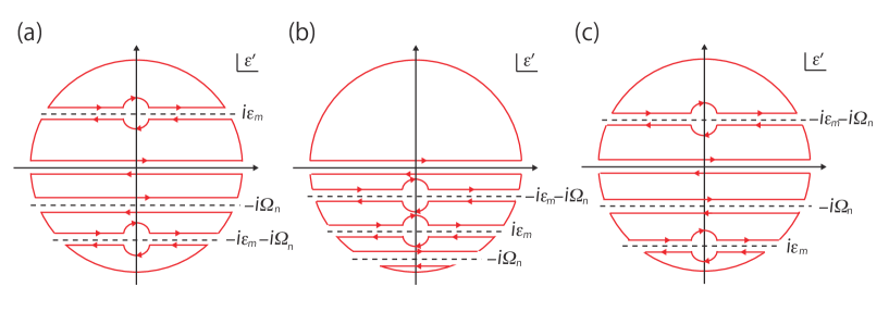
Figure 22: Contours used for the analytic continuations of the three-point vector vertex function. $\textrm{Im}\epsilon>0$ and $\textrm{Im}\epsilon+\textrm{Im}\omega>0$ are satisfied in panel (a), $\textrm{Im}\epsilon<0$ and $\textrm{Im}\epsilon+\textrm{Im}\omega>0$ are satisfied in panel (b), and $\textrm{Im}\epsilon<0$ and $\textrm{Im}\epsilon+\textrm{Im}\omega<0$ are satisfied in panel (c).

In this appendix, we derive Eq. (16) after defining the three-point vector vertex function in Matsubara-frequency representation and carrying out its analytic continuation.

We can express Eq. (13) in a more compact form since $\mathcal{J}_{ll^{\prime};\{A\}}(k,k^{\prime};\omega)$ are connected with the three-point vector vertex function in real-frequency representation. We begin with the definition Takada-text in Matsubara-frequency representation, $\Lambda_{\nu;AB}(\bm{k},i\epsilon_{m};\bm{q},i\Omega_{n})\equiv\Lambda_{\nu;AB}(\bm{k}+\bm{q},i\epsilon_{m+n},\bm{k},i\epsilon_{m})$:

$$\textstyle\sum\limits_{A,B}G_{aA}(\bm{k}+\bm{q},i\epsilon_{m+n})\Lambda_{\nu;AB}(\bm{k},i\epsilon_{m};\bm{q},i\Omega_{n})G_{Bb}(\bm{k},i\epsilon_{m})$$

$$= \int^{T^{-1}}_{0}d\tau e^{i\epsilon_{m+n}\tau}\int^{T^{-1}}_{0}d\tau^{\prime}e^{-i\Omega_{n}\tau^{\prime}}\langle\textrm{T}_{\tau}\hat{c}_{\bm{k}+\bm{q}a}(\tau)\hat{J}_{-\bm{q}\nu}(\tau^{\prime})\hat{c}_{\bm{k}b}^{\dagger}\rangle.$$ (94)

After some algebra for Eq. (94), we obtain the Bethe-Salpeter equation to determine $\Lambda_{\nu;AB}(\bm{k},i\epsilon_{m};\bm{q},i\Omega_{n})$,

$$\Lambda_{\nu;ab}(\bm{k},i\epsilon_{m};\bm{q},i\Omega_{n})=(v_{\bm{k}\nu})_{ab}$$

$$+\frac{T}{N}\sum\limits_{\bm{k}^{\prime}}\sum\limits_{m^{\prime}}\sum\limits_{\{A\}}\Gamma_{abCD}(\bm{k},i\epsilon_{m},\bm{k}^{\prime}i\epsilon_{m^{\prime}};\bm{q},i\Omega_{n})$$

$$\times G_{CA}(\bm{k}^{\prime}+\bm{q},i\epsilon_{m^{\prime}+n})G_{BD}(\bm{k}^{\prime},i\epsilon_{m^{\prime}})(v_{\bm{k}^{\prime}\nu})_{AB}.$$ (95)

Since the second term of Eq. (95) has the similar analytic property for the second term of Eq. (10), we can similarly carry out the analytic continuation of the former as follows:

$$\frac{T}{N}\sum\limits_{\bm{k}^{\prime}}\sum\limits_{m^{\prime}}\sum\limits_{\{A\}}\Gamma_{abCD}(\bm{k},i\epsilon_{m},\bm{k}^{\prime}i\epsilon_{m^{\prime}};\bm{q},i\Omega_{n})G_{CA}(\bm{k}^{\prime}+\bm{q},i\epsilon_{m^{\prime}+n})G_{BD}(\bm{k}^{\prime},i\epsilon_{m^{\prime}})(v_{\bm{k}^{\prime}\nu})_{AB}$$

$$=\ \frac{1}{N}\sum\limits_{\bm{k}^{\prime}}\sum\limits_{\{A\}}\Bigl{[}\int_{C^{\prime}}\frac{d\epsilon^{\prime}}{4\pi i}\tanh\frac{\epsilon^{\prime}}{2T}\Gamma_{abCD}(\bm{k},i\epsilon_{m},\bm{k}^{\prime},\epsilon^{\prime};\bm{q},i\Omega_{n})G_{CA}(\bm{k}^{\prime}+\bm{q},\epsilon^{\prime}+i\Omega_{n})G_{BD}(\bm{k}^{\prime},\epsilon^{\prime})$$

$$\ \ \ \ \ \ \ \ \ \ \ \ +T\Gamma_{abCD}(\bm{k},i\epsilon_{m},\bm{k}^{\prime},i\epsilon_{m};\bm{q},i\Omega_{n})G_{CA}(\bm{k}^{\prime}+\bm{q},i\epsilon_{m}+i\Omega_{n})G_{BD}(\bm{k}^{\prime},i\epsilon_{m})$$

$$\ \ \ \ \ \ \ \ \ \ \ \ +T\Gamma_{abCD}(\bm{k},i\epsilon_{m},\bm{k}^{\prime},-i\epsilon_{m}-i\Omega_{n};\bm{q},i\Omega_{n})G_{CA}(\bm{k}^{\prime}+\bm{q},-i\epsilon_{m})G_{BD}(\bm{k}^{\prime},-i\epsilon_{m}-i\Omega_{n})\Bigr{]}(v_{\bm{k}^{\prime}\nu})_{AB},$$ (96)

where the contour $C^{\prime}$ is the contour shown in Fig. 22(a) or 22(b) or 22(c), depending on the values of $\textrm{Im}\epsilon$ and $\textrm{Im}\epsilon+\textrm{Im}\omega$ for the second term of Eq. (95). Thus, the three-point vector vertex function in real-frequency representation is given by

$$\Lambda_{\nu;l;ab}(k;q)=\ (v_{\bm{k}\nu})_{ab}$$

$$+\frac{1}{N}\sum\limits_{\bm{k}^{\prime}}\sum\limits_{\{A\}}\sum\limits_{l^{\prime}=1}^{3}\int^{\infty}_{-\infty}\frac{d\epsilon^{\prime}}{4\pi i}\mathcal{J}_{ll^{\prime};abCD}(k,k^{\prime};q)$$

$$\times g_{l^{\prime};CABD}(k^{\prime};q)(v_{\bm{k}^{\prime}\nu})_{AB},$$ (97)

where case for $l=1$ or $2$ or $3$ corresponds to case of Fig. 22(a) or 22(b) or 22(c), respectively. Using Eqs. (13), (14), and (97), we can rewrite Eq. (13) as Eq. (16).

Appendix C Derivation of Eq. (36)

In this appendix, I explain the detail of the derivation of the $\bm{q}$-linear terms of $K_{xy\nu}(\bm{q},i\Omega_{n})$ in the most-divergent-term approximation Fukuyama-RH ; Kohno-Yamada .

We start to show the leading-order $\bm{q}$ dependence of each quantity appearing in Eq. (35). First, $G_{aA}(\bm{k}_{-},i\epsilon_{m})G_{Bb}(\bm{k}_{+},i\epsilon_{m+n})$ is approximated within the linear order of $\bm{q}$ as

$$G_{aA}(\bm{k}_{-},i\epsilon_{m})G_{Bb}(\bm{k}_{+},i\epsilon_{m+n})$$

$$\sim \ G_{aA}(\bm{k},i\epsilon_{m})G_{Bb}(\bm{k},i\epsilon_{m+n})$$

$$+\sum\limits_{\eta}\dfrac{q_{\eta}}{2}\Bigl{[}G_{aA}(\bm{k},i\epsilon_{m})\dfrac{\overleftrightarrow{\partial}}{\partial k_{\eta}}G_{Bb}(\bm{k},i\epsilon_{m+n})\Bigr{]},$$ (98)

where we introduce a quantity,

$$\Bigl{[}g(x)\dfrac{\overleftrightarrow{\partial}}{\partial x}h(x)\Bigr{]}\equiv g(x)\dfrac{\partial h(x)}{\partial x}-\dfrac{\partial h(x)}{\partial x}h(x).$$ (99)

Second, $\Lambda_{y;dc}(\bm{k}_{\pm},i\epsilon_{m+n},\bm{k}_{\pm},i\epsilon_{m})$ is approximated as

$$\Lambda_{y;dc}(\bm{k}_{\pm},i\epsilon_{m+n},\bm{k}_{\pm},i\epsilon_{m})\sim\ \Lambda_{y;dc}(\bm{k},i\epsilon_{m+n},\bm{k},i\epsilon_{m})$$

$$\pm\sum\limits_{\eta}\dfrac{q_{\eta}}{2}\dfrac{\partial}{\partial k_{\eta}}\Lambda_{y;dc}(\bm{k},i\epsilon_{m+n},\bm{k},i\epsilon_{m}).$$ (100)

Third, the leading-order $\bm{q}$ dependence of $\Lambda_{x;AB}(\bm{k}_{-},i\epsilon_{m},\bm{k}_{+},i\epsilon_{m+n})$ is given by

$$\Lambda_{x;AB}(\bm{k}_{-},i\epsilon_{m},\bm{k}_{+},i\epsilon_{m+n})\sim\ \Lambda_{x;AB}(\bm{k},i\epsilon_{m},\bm{k},i\epsilon_{m+n})$$

$$+\Delta\Lambda_{x;AB}(\bm{k},i\epsilon_{m},\bm{k},i\epsilon_{m+n}),$$ (101)

with the equation derived from Eq. (95),

$$\Delta\Lambda_{x;AB}(\bm{k},i\epsilon_{m},\bm{k},i\epsilon_{m+n})$$

$$= \frac{T}{N}\sum\limits_{\bm{k}^{\prime}}\sum\limits_{m^{\prime}}\sum\limits_{\{a\}}\Gamma_{ABcd}^{(1)}(\bm{k},i\epsilon_{m},\bm{k},i\epsilon_{m+n};\bm{k}^{\prime},i\epsilon_{m^{\prime}},\bm{k}^{\prime},i\epsilon_{m^{\prime}+n})$$

$$\times\sum\limits_{\eta}\dfrac{q_{\eta}}{2}\Bigl{[}G_{ca}(\bm{k}^{\prime},i\epsilon_{m^{\prime}})\dfrac{\overleftrightarrow{\partial}}{\partial k_{\eta}}G_{bd}(\bm{k}^{\prime},i\epsilon_{m^{\prime}+n})\Bigr{]}$$

$$\times\Lambda_{x;ab}(\bm{k}^{\prime},i\epsilon_{m^{\prime}},\bm{k}^{\prime},i\epsilon_{m^{\prime}+n})$$

$$+\frac{T}{N}\sum\limits_{\bm{k}^{\prime}}\sum\limits_{m^{\prime}}\sum\limits_{\{a\}}\Gamma_{ABcd}^{(1)}(\bm{k},i\epsilon_{m},\bm{k},i\epsilon_{m+n};\bm{k}^{\prime},i\epsilon_{m^{\prime}},\bm{k}^{\prime},i\epsilon_{m^{\prime}+n})$$

$$\times G_{bd}(\bm{k}^{\prime},i\epsilon_{m^{\prime}+n})G_{ca}(\bm{k}^{\prime},i\epsilon_{m^{\prime}})$$

$$\times\Delta\Lambda_{x;ab}(\bm{k}^{\prime},i\epsilon_{m^{\prime}},\bm{k}^{\prime},i\epsilon_{m^{\prime}+n}).$$ (102)

In Eq. (102), we have neglected the $\bm{q}$-linear term arising from the irreducible four-point vertex function because that is negligible compared with the main terms in the most-divergent-term approximation Fukuyama-RH ; Kohno-Yamada . Fourth, due to the same reason, we can neglect the $\bm{q}$-linear term arising from the irreducible six-point vertex function Fukuyama-RH ; Kohno-Yamada . Fifth, the $\bm{q}$ dependence of $\sum_{f,g}G_{fb}(\bm{k}_{-},i\epsilon_{m})\Lambda_{\nu;gf}(\bm{k}_{+},i\epsilon_{m},\bm{k}_{-},i\epsilon_{m})G_{cg}(\bm{k}_{+},i\epsilon_{m})$ is negligible in the most-divergent-term approximation Fukuyama-RH ; Kohno-Yamada since we can neglect the $\bm{q}$-linear term arising from a pair of two single-particle Green’s functions whose frequencies are the same in the most-divergent-term approximation Fukuyama-RH ; Kohno-Yamada . More precisely, $\sum_{f,g}G_{fb}(\bm{k}_{-},i\epsilon_{m})\Lambda_{\nu;gf}(\bm{k}_{+},i\epsilon_{m},\bm{k}_{-},i\epsilon_{m})G_{cg}(\bm{k}_{+},i\epsilon_{m})$ is approximated as

$$\sum\limits_{f,g}G_{fb}(\bm{k}_{-},i\epsilon_{m})\Lambda_{\alpha;gf}(\bm{k}_{+},i\epsilon_{m},\bm{k}_{-},i\epsilon_{m})G_{cg}(\bm{k}_{+},i\epsilon_{m})$$

$$\sim \ \textstyle\sum\limits_{f,g}G_{fb}(\bm{k},i\epsilon_{m})\Lambda_{\alpha;gf}(\bm{k},i\epsilon_{m},\bm{k},i\epsilon_{m})G_{cg}(\bm{k},i\epsilon_{m})$$

$$= \ \dfrac{\partial G_{cb}(\bm{k},i\epsilon_{m})}{\partial k_{\alpha}}.$$ (103)

In the final line, we use one of the Ward identities Fukuyama-RH ; Kohno-Yamada .

Using the $\bm{q}$ dependences of the quantities appearing in Eq. (35), we obtain the $\bm{q}$-linear terms of $K_{xy\nu}(\bm{q},i\Omega_{n})$ in the most-divergent-term approximation Fukuyama-RH ; Kohno-Yamada :

$$K_{xy\nu}(\bm{q},i\Omega_{n})= \ \delta_{\nu,y}\frac{T}{N}\sum\limits_{\bm{k}}\sum\limits_{m}\sum\limits_{a,b,A,B}\dfrac{\partial(v_{\bm{k}y})_{ba}}{\partial k_{\nu}}G_{aA}(\bm{k},i\epsilon_{m})\Delta\Lambda_{x;AB}(\bm{k},i\epsilon_{m},\bm{k},i\epsilon_{m+n})G_{Bb}(\bm{k},i\epsilon_{m+n})$$

$$+\delta_{\nu,y}\frac{T}{N}\sum\limits_{\bm{k}}\sum\limits_{m}\sum\limits_{a,b,A,B}\dfrac{\partial(v_{\bm{k}y})_{ba}}{\partial k_{\nu}}\Lambda_{x;AB}(\bm{k},i\epsilon_{m},\bm{k},i\epsilon_{m+n})\sum\limits_{\eta}\dfrac{q_{\eta}}{2}\Bigl{[}G_{aA}(\bm{k},i\epsilon_{m})\dfrac{\overleftrightarrow{\partial}}{\partial k_{\eta}}G_{Bb}(\bm{k},i\epsilon_{m+n})\Bigr{]}$$

$$+\frac{T}{N}\sum\limits_{\bm{k}}\sum\limits_{m}\sum\limits_{\{a\}}\Delta\Lambda_{x;ba}(\bm{k},i\epsilon_{m},\bm{k},i\epsilon_{m+n})G_{ad}(\bm{k},i\epsilon_{m+n})\dfrac{\partial G_{cb}(\bm{k},i\epsilon_{m})}{\partial k_{\nu}}\Lambda_{y;dc}(\bm{k},i\epsilon_{m+n},\bm{k},i\epsilon_{m})$$

$$+\frac{T}{N}\sum\limits_{\bm{k}}\sum\limits_{m}\sum\limits_{\{a\}}\Lambda_{x;ba}(\bm{k},i\epsilon_{m},\bm{k},i\epsilon_{m+n})\sum\limits_{\eta}\dfrac{q_{\eta}}{2}\dfrac{\partial G_{ad}(\bm{k},i\epsilon_{m+n})}{\partial k_{\eta}}\dfrac{\partial G_{cb}(\bm{k},i\epsilon_{m})}{\partial k_{\nu}}\Lambda_{y;dc}(\bm{k},i\epsilon_{m+n},\bm{k},i\epsilon_{m})$$

$$+\frac{T}{N}\sum\limits_{\bm{k}}\sum\limits_{m}\sum\limits_{\{a\}}\Lambda_{x;ba}(\bm{k},i\epsilon_{m},\bm{k},i\epsilon_{m+n})G_{ad}(\bm{k},i\epsilon_{m+n})\dfrac{\partial G_{cb}(\bm{k},i\epsilon_{m})}{\partial k_{\nu}}\sum\limits_{\eta}\dfrac{q_{\eta}}{2}\dfrac{\partial\Lambda_{y;dc}(\bm{k},i\epsilon_{m+n},\bm{k},i\epsilon_{m})}{\partial k_{\eta}}$$

$$+\frac{T}{N}\sum\limits_{\bm{k}}\sum\limits_{m}\sum\limits_{\{a\}}\Delta\Lambda_{x;ba}(\bm{k},i\epsilon_{m},\bm{k},i\epsilon_{m+n})G_{cb}(\bm{k},i\epsilon_{m})\dfrac{\partial G_{ad}(\bm{k},i\epsilon_{m+n})}{\partial k_{\nu}}\Lambda_{y;dc}(\bm{k},i\epsilon_{m+n},\bm{k},i\epsilon_{m})$$

$$-\frac{T}{N}\sum\limits_{\bm{k}}\sum\limits_{m}\sum\limits_{\{a\}}\Lambda_{x;ba}(\bm{k},i\epsilon_{m},\bm{k},i\epsilon_{m+n})\sum\limits_{\eta}\dfrac{q_{\eta}}{2}\dfrac{\partial G_{cb}(\bm{k},i\epsilon_{m})}{\partial k_{\eta}}\dfrac{\partial G_{ad}(\bm{k},i\epsilon_{m+n})}{\partial k_{\nu}}\Lambda_{y;dc}(\bm{k},i\epsilon_{m+n},\bm{k},i\epsilon_{m})$$

$$-\frac{T}{N}\sum\limits_{\bm{k}}\sum\limits_{m}\sum\limits_{\{a\}}\Lambda_{x;ba}(\bm{k},i\epsilon_{m},\bm{k},i\epsilon_{m+n})G_{cb}(\bm{k},i\epsilon_{m})\dfrac{\partial G_{ad}(\bm{k},i\epsilon_{m+n})}{\partial k_{\nu}}\sum\limits_{\eta}\dfrac{q_{\eta}}{2}\dfrac{\partial\Lambda_{y;dc}(\bm{k},i\epsilon_{m+n},\bm{k},i\epsilon_{m})}{\partial k_{\eta}}$$

$$+\Bigl{(}\frac{T}{N}\Bigr{)}^{3}\sum\limits_{\bm{k},\bm{k}^{\prime},\bm{k}^{\prime\prime}}\sum\limits_{m,m^{\prime},m^{\prime\prime}}\sum\limits_{\{a\}}\sum\limits_{\{A\}}\sum\limits_{F,G}G_{Bb}(\bm{k},i\epsilon_{m})\Delta\Lambda_{x;ba}(\bm{k},i\epsilon_{m},\bm{k},i\epsilon_{m+n})G_{aA}(\bm{k},i\epsilon_{m+n})$$

$$\ \ \times\dfrac{\partial G_{GF}(\bm{k}^{\prime\prime},i\epsilon_{m^{\prime\prime}})}{\partial k^{\prime\prime}_{\nu}}G_{Dd}(\bm{k}^{\prime},i\epsilon_{m^{\prime}+n})\Lambda_{y;dc}(\bm{k}^{\prime},i\epsilon_{m^{\prime}+n},\bm{k}^{\prime},i\epsilon_{m^{\prime}})G_{cC}(\bm{k}^{\prime},i\epsilon_{m^{\prime}})$$

$$\ \ \times\Gamma_{3;ABCDFG}^{(1)}(\bm{k},i\epsilon_{m+n},\bm{k},i\epsilon_{m};\bm{k}^{\prime},i\epsilon_{m^{\prime}},\bm{k}^{\prime},i\epsilon_{m^{\prime}+n};\bm{k}^{\prime\prime},i\epsilon_{m^{\prime\prime}},\bm{k}^{\prime\prime},i\epsilon_{m^{\prime\prime}})$$

$$+\Bigl{(}\frac{T}{N}\Bigr{)}^{3}\sum\limits_{\bm{k},\bm{k}^{\prime},\bm{k}^{\prime\prime}}\sum\limits_{m,m^{\prime},m^{\prime\prime}}\sum\limits_{\{a\}}\sum\limits_{\{A\}}\sum\limits_{F,G}\Lambda_{x;ba}(\bm{k},i\epsilon_{m},\bm{k},i\epsilon_{m+n})\sum\limits_{\eta}\dfrac{q_{\eta}}{2}\Bigl{[}G_{Bb}(\bm{k},i\epsilon_{m})\dfrac{\overleftrightarrow{\partial}}{\partial k_{\eta}}G_{aA}(\bm{k},i\epsilon_{m+n})\Bigr{]}$$

$$\ \ \times\dfrac{\partial G_{GF}(\bm{k}^{\prime\prime},i\epsilon_{m^{\prime\prime}})}{\partial k^{\prime\prime}_{\nu}}G_{Dd}(\bm{k}^{\prime},i\epsilon_{m^{\prime}+n})\Lambda_{y;dc}(\bm{k}^{\prime},i\epsilon_{m^{\prime}+n},\bm{k}^{\prime},i\epsilon_{m^{\prime}})G_{cC}(\bm{k}^{\prime},i\epsilon_{m^{\prime}})$$

$$\ \ \times\Gamma_{3;ABCDFG}^{(1)}(\bm{k},i\epsilon_{m+n},\bm{k},i\epsilon_{m};\bm{k}^{\prime},i\epsilon_{m^{\prime}},\bm{k}^{\prime},i\epsilon_{m^{\prime}+n};\bm{k}^{\prime\prime},i\epsilon_{m^{\prime\prime}},\bm{k}^{\prime\prime},i\epsilon_{m^{\prime\prime}}).$$ (104)

The above ninth and tenth terms can be rewritten in a simpler form by using Eqs. (95) and (102), the exchange symmetry Kohno-Yamada of the four-point vertex function, and the relation Kohno-Yamada between the irreducible four-point and the irreducible six-point vertex function,

$$\Bigl{(}\dfrac{\partial}{\partial k_{\nu}}+\dfrac{\partial}{\partial k^{\prime}_{\nu}}\Bigr{)}\Gamma_{ABDC}^{(1)}(\bm{k},i\epsilon_{m+n},\bm{k},i\epsilon_{m};\bm{k}^{\prime},i\epsilon_{m^{\prime}+n},\bm{k}^{\prime},i\epsilon_{m^{\prime}})$$

$$= \ \frac{T}{N}\sum\limits_{\bm{k}^{\prime\prime}}\sum\limits_{m^{\prime\prime}}\sum\limits_{F,G}\Gamma_{3;ABCDFG}^{(1)}(\bm{k},i\epsilon_{m+n},\bm{k},i\epsilon_{m};\bm{k}^{\prime},i\epsilon_{m^{\prime}},\bm{k}^{\prime},i\epsilon_{m^{\prime}+n};\bm{k}^{\prime\prime},i\epsilon_{m^{\prime\prime}},\bm{k}^{\prime\prime},i\epsilon_{m^{\prime\prime}})\dfrac{\partial G_{GF}(\bm{k}^{\prime\prime},i\epsilon_{m^{\prime\prime}})}{\partial k^{\prime\prime}_{\nu}}.$$ (105)

Namely, the ninth and tenth terms become

$$\ \ \Bigl{(}\frac{T}{N}\Bigr{)}^{2}\sum\limits_{\bm{k},\bm{k}^{\prime}}\sum\limits_{m,m^{\prime}}\sum\limits_{\{a\}}\sum\limits_{\{A\}}G_{Bb}(\bm{k},i\epsilon_{m})\Delta\Lambda_{x;ba}(\bm{k},i\epsilon_{m},\bm{k},i\epsilon_{m+n})G_{aA}(\bm{k},i\epsilon_{m+n})G_{Dd}(\bm{k}^{\prime},i\epsilon_{m^{\prime}+n})$$

$$\ \ \times\Lambda_{y;dc}(\bm{k}^{\prime},i\epsilon_{m^{\prime}+n},\bm{k}^{\prime},i\epsilon_{m^{\prime}})G_{cC}(\bm{k}^{\prime},i\epsilon_{m^{\prime}})\Bigl{(}\dfrac{\partial}{\partial k_{\nu}}+\dfrac{\partial}{\partial k^{\prime}_{\nu}}\Bigr{)}\Gamma_{ABDC}^{(1)}(\bm{k},i\epsilon_{m+n},\bm{k},i\epsilon_{m};\bm{k}^{\prime},i\epsilon_{m^{\prime}+n},\bm{k}^{\prime},i\epsilon_{m^{\prime}})$$

$$+\Bigl{(}\frac{T}{N}\Bigr{)}^{2}\sum\limits_{\bm{k},\bm{k}^{\prime}}\sum\limits_{m,m^{\prime}}\sum\limits_{\{a\}}\sum\limits_{\{A\}}\Lambda_{x;ba}(\bm{k},i\epsilon_{m},\bm{k},i\epsilon_{m+n})\sum\limits_{\eta}\dfrac{q_{\eta}}{2}\Bigl{[}G_{Bb}(\bm{k},i\epsilon_{m})\dfrac{\overleftrightarrow{\partial}}{\partial k_{\eta}}G_{aA}(\bm{k},i\epsilon_{m+n})\Bigr{]}G_{Dd}(\bm{k}^{\prime},i\epsilon_{m^{\prime}+n})$$

$$\ \ \times\Lambda_{y;dc}(\bm{k}^{\prime},i\epsilon_{m^{\prime}+n},\bm{k}^{\prime},i\epsilon_{m^{\prime}})G_{cC}(\bm{k}^{\prime},i\epsilon_{m^{\prime}})\Bigl{(}\dfrac{\partial}{\partial k_{\nu}}+\dfrac{\partial}{\partial k^{\prime}_{\nu}}\Bigr{)}\Gamma_{ABDC}^{(1)}(\bm{k},i\epsilon_{m+n},\bm{k},i\epsilon_{m};\bm{k}^{\prime},i\epsilon_{m^{\prime}+n},\bm{k}^{\prime},i\epsilon_{m^{\prime}})$$

$$=\ \frac{T}{N}\sum\limits_{\bm{k}}\sum\limits_{m}\sum\limits_{a,b,A,B}G_{Bb}(\bm{k},i\epsilon_{m})\Delta\Lambda_{x;ba}(\bm{k},i\epsilon_{m},\bm{k},i\epsilon_{m+n})G_{aA}(\bm{k},i\epsilon_{m+n})\dfrac{\partial}{\partial k_{\nu}}\Bigl{[}\Lambda_{y;AB}(\bm{k},i\epsilon_{m+n},\bm{k},i\epsilon_{m})-(v_{\bm{k}y})_{AB}\Bigr{]}$$

$$- \Bigl{(}\frac{T}{N}\Bigr{)}^{2}\sum\limits_{\bm{k},\bm{k}^{\prime}}\sum\limits_{m,m^{\prime}}\sum\limits_{\{a\}}\sum\limits_{\{A\}}G_{Bb}(\bm{k},i\epsilon_{m})\Delta\Lambda_{x;ba}(\bm{k},i\epsilon_{m},\bm{k},i\epsilon_{m+n})G_{aA}(\bm{k},i\epsilon_{m+n})$$

$$\times\dfrac{\partial}{\partial k^{\prime}_{\nu}}\Bigl{[}G_{Dd}(\bm{k}^{\prime},i\epsilon_{m^{\prime}+n})\Lambda_{y;dc}(\bm{k}^{\prime},i\epsilon_{m^{\prime}+n},\bm{k}^{\prime},i\epsilon_{m^{\prime}})G_{cC}(\bm{k}^{\prime},i\epsilon_{m^{\prime}})\Bigr{]}\Gamma_{ABDC}^{(1)}(\bm{k},i\epsilon_{m+n},\bm{k},i\epsilon_{m};\bm{k}^{\prime},i\epsilon_{m^{\prime}+n},\bm{k}^{\prime},i\epsilon_{m^{\prime}})$$

$$+ \frac{T}{N}\sum\limits_{\bm{k}}\sum\limits_{m}\sum\limits_{a,b,A,B}\Lambda_{x;ba}(\bm{k},i\epsilon_{m},\bm{k},i\epsilon_{m+n})\sum\limits_{\eta}\dfrac{q_{\eta}}{2}\Bigl{[}G_{Bb}(\bm{k},i\epsilon_{m})\dfrac{\overleftrightarrow{\partial}}{\partial k_{\eta}}G_{aA}(\bm{k},i\epsilon_{m+n})\Bigr{]}$$

$$\times\dfrac{\partial}{\partial k_{\nu}}\Bigl{[}\Lambda_{y;AB}(\bm{k},i\epsilon_{m+n},\bm{k},i\epsilon_{m})-(v_{\bm{k}y})_{AB}\Bigr{]}$$

$$- \Bigl{(}\frac{T}{N}\Bigr{)}^{2}\sum\limits_{\bm{k},\bm{k}^{\prime}}\sum\limits_{m,m^{\prime}}\sum\limits_{\{a\}}\sum\limits_{\{A\}}\Lambda_{x;ba}(\bm{k},i\epsilon_{m},\bm{k},i\epsilon_{m+n})\sum\limits_{\eta}\dfrac{q_{\eta}}{2}\Bigl{[}G_{Bb}(\bm{k},i\epsilon_{m})\dfrac{\overleftrightarrow{\partial}}{\partial k_{\eta}}G_{aA}(\bm{k},i\epsilon_{m+n})\Bigr{]}$$

$$\times\dfrac{\partial}{\partial k^{\prime}_{\nu}}\Bigl{[}G_{Dd}(\bm{k}^{\prime},i\epsilon_{m^{\prime}+n})\Lambda_{y;dc}(\bm{k}^{\prime},i\epsilon_{m^{\prime}+n},\bm{k}^{\prime},i\epsilon_{m^{\prime}})G_{cC}(\bm{k}^{\prime},i\epsilon_{m^{\prime}})\Bigr{]}\Gamma_{ABDC}^{(1)}(\bm{k},i\epsilon_{m+n},\bm{k},i\epsilon_{m};\bm{k}^{\prime},i\epsilon_{m^{\prime}+n},\bm{k}^{\prime},i\epsilon_{m^{\prime}})$$

$$=\ \frac{T}{N}\sum\limits_{\bm{k}}\sum\limits_{m}\sum\limits_{a,b,A,B}\Bigl{\{}\Delta\Lambda_{x;ba}(\bm{k},i\epsilon_{m},\bm{k},i\epsilon_{m+n})G_{Bb}(\bm{k},i\epsilon_{m})G_{aA}(\bm{k},i\epsilon_{m+n})$$

$$\ \ \ \ \ \ \ \ \ \ \ \ \ \ \ \ +\Lambda_{x;ba}(\bm{k},i\epsilon_{m},\bm{k},i\epsilon_{m+n})\sum\limits_{\eta}\dfrac{q_{\eta}}{2}\Bigl{[}G_{Bb}(\bm{k},i\epsilon_{m})\dfrac{\overleftrightarrow{\partial}}{\partial k_{\eta}}G_{aA}(\bm{k},i\epsilon_{m+n})\Bigr{]}\Bigr{\}}$$

$$\ \ \ \ \ \ \ \ \ \ \ \ \ \ \ \ \times\dfrac{\partial}{\partial k_{\nu}}\Bigl{[}\Lambda_{y;AB}(\bm{k},i\epsilon_{m+n},\bm{k},i\epsilon_{m})-(v_{\bm{k}y})_{AB}\Bigr{]}$$

$$- \frac{T}{N}\sum\limits_{\bm{k}}\sum\limits_{m}\sum\limits_{c,d,C,D}\Delta\Lambda_{x;DC}(\bm{k}^{\prime},i\epsilon_{m^{\prime}+n},\bm{k}^{\prime},i\epsilon_{m^{\prime}})\dfrac{\partial}{\partial k^{\prime}_{\nu}}\Bigl{[}G_{Dd}(\bm{k}^{\prime},i\epsilon_{m^{\prime}+n})\Lambda_{y;dc}(\bm{k}^{\prime},i\epsilon_{m^{\prime}+n},\bm{k}^{\prime},i\epsilon_{m^{\prime}})G_{cC}(\bm{k}^{\prime},i\epsilon_{m^{\prime}})\Bigr{]}.$$ (106)

Thus, replacing the ninth and tenth terms of Eq. (104) by the terms of Eq. (106), we can rewrite Eq. (104) in a simpler form:

$$K_{xy\nu}(\bm{q},i\Omega_{n})= \frac{T}{N}\sum\limits_{\bm{k}}\sum\limits_{m}\sum\limits_{\{a\}}\Lambda_{x;ba}(\bm{k},i\epsilon_{m},\bm{k},i\epsilon_{m+n})\sum\limits_{\eta}\dfrac{q_{\eta}}{2}\dfrac{\partial G_{ad}(\bm{k},i\epsilon_{m+n})}{\partial k_{\eta}}\dfrac{\partial G_{cb}(\bm{k},i\epsilon_{m})}{\partial k_{\nu}}\Lambda_{y;dc}(\bm{k},i\epsilon_{m+n};\bm{k},i\epsilon_{m})$$

$$+\frac{T}{N}\sum\limits_{\bm{k}}\sum\limits_{m}\sum\limits_{\{a\}}\Lambda_{x;ba}(\bm{k},i\epsilon_{m},\bm{k},i\epsilon_{m+n})G_{ad}(\bm{k},i\epsilon_{m+n})\dfrac{\partial G_{cb}(\bm{k},i\epsilon_{m})}{\partial k_{\nu}}\sum\limits_{\eta}\dfrac{q_{\eta}}{2}\dfrac{\partial\Lambda_{y;dc}(\bm{k},i\epsilon_{m+n},\bm{k},i\epsilon_{m})}{\partial k_{\eta}}$$

$$-\frac{T}{N}\sum\limits_{\bm{k}}\sum\limits_{m}\sum\limits_{\{a\}}\Lambda_{x;ba}(\bm{k},i\epsilon_{m},\bm{k},i\epsilon_{m+n})\sum\limits_{\eta}\dfrac{q_{\eta}}{2}\dfrac{\partial G_{cb}(\bm{k},i\epsilon_{m})}{\partial k_{\eta}}\dfrac{\partial G_{ad}(\bm{k},i\epsilon_{m+n})}{\partial k_{\nu}}\Lambda_{y;dc}(\bm{k},i\epsilon_{m+n},\bm{k},i\epsilon_{m})$$

$$-\frac{T}{N}\sum\limits_{\bm{k}}\sum\limits_{m}\sum\limits_{\{a\}}\Lambda_{x;ba}(\bm{k},i\epsilon_{m},\bm{k},i\epsilon_{m+n})G_{cb}(\bm{k},i\epsilon_{m})\dfrac{\partial G_{ad}(\bm{k},i\epsilon_{m+n})}{\partial k_{\nu}}\sum\limits_{\eta}\dfrac{q_{\eta}}{2}\dfrac{\partial\Lambda_{y;dc}(\bm{k},i\epsilon_{m+n},\bm{k},i\epsilon_{m})}{\partial k_{\eta}}$$

$$+\frac{T}{N}\sum\limits_{\bm{k}}\sum\limits_{m}\sum\limits_{\{a\}}\Lambda_{x;ba}(\bm{k},i\epsilon_{m},\bm{k},i\epsilon_{m+n})\sum\limits_{\eta}\dfrac{q_{\eta}}{2}\Bigl{[}G_{cb}(\bm{k},i\epsilon_{m})\dfrac{\overleftrightarrow{\partial}}{\partial k_{\eta}}G_{ad}(\bm{k},i\epsilon_{m+n})\Bigr{]}$$

$$\ \times\dfrac{\partial\Lambda_{y;dc}(\bm{k},i\epsilon_{m+n},\bm{k},i\epsilon_{m})}{\partial k_{\nu}}$$

$$=\frac{T}{N}\sum\limits_{\bm{k}}\sum\limits_{m}\sum\limits_{\{a\}}\Lambda_{x;ba}(\bm{k},i\epsilon_{m},\bm{k},i\epsilon_{m+n})\Lambda_{y;dc}(\bm{k},i\epsilon_{m+n},\bm{k},i\epsilon_{m})$$

$$\ \ \ \ \times\sum\limits_{\eta}\dfrac{q_{\eta}}{2}\Bigl{\{}\dfrac{\partial G_{ad}(\bm{k},i\epsilon_{m+n})}{\partial k_{\eta}}\dfrac{\partial G_{cb}(\bm{k},i\epsilon_{m})}{\partial k_{\nu}}-\dfrac{\partial G_{ad}(\bm{k},i\epsilon_{m+n})}{\partial k_{\nu}}\dfrac{\partial G_{cb}(\bm{k},i\epsilon_{m})}{\partial k_{\eta}}\Bigr{\}}$$

$$+\frac{T}{N}\sum\limits_{\bm{k}}\sum\limits_{m}\sum\limits_{\{a\}}\Lambda_{x;ba}(\bm{k},i\epsilon_{m},\bm{k},i\epsilon_{m+n})$$

$$\ \ \times\sum\limits_{\eta}\dfrac{q_{\eta}}{2}\Bigl{\{}\Bigl{[}G_{cb}(\bm{k},i\epsilon_{m})\dfrac{\overleftrightarrow{\partial}}{\partial k_{\eta}}G_{ad}(\bm{k},i\epsilon_{m+n})\Bigr{]}\dfrac{\partial\Lambda_{y;dc}(\bm{k},i\epsilon_{m+n},\bm{k},i\epsilon_{m})}{\partial k_{\nu}}$$

$$\ \ \ \ \ \ \ \ \ \ \ \ \ -\Bigl{[}G_{cb}(\bm{k},i\epsilon_{m})\dfrac{\overleftrightarrow{\partial}}{\partial k_{\nu}}G_{ad}(\bm{k},i\epsilon_{m+n})\Bigr{]}\dfrac{\partial\Lambda_{y;dc}(\bm{k},i\epsilon_{m+n},\bm{k},i\epsilon_{m})}{\partial k_{\eta}}\Bigr{\}}$$

$$=\frac{1}{2}(q_{x}\delta_{\nu,y}-q_{y}\delta_{\nu,x})\frac{T}{N}\sum\limits_{\bm{k}}\sum\limits_{m}\sum\limits_{\{a\}}\Lambda_{x;ba}(\bm{k},i\epsilon_{m},\bm{k},i\epsilon_{m+n})$$

$$\ \ \times\Bigl{\{}\Bigl{[}G_{cb}(\bm{k},i\epsilon_{m})\dfrac{\overleftrightarrow{\partial}}{\partial k_{x}}G_{ad}(\bm{k},i\epsilon_{m+n})\Bigr{]}\dfrac{\partial\Lambda_{y;dc}(\bm{k},i\epsilon_{m+n},\bm{k},i\epsilon_{m})}{\partial k_{y}}$$

$$\ \ \ \ \ \ -\Bigl{[}G_{cb}(\bm{k},i\epsilon_{m})\dfrac{\overleftrightarrow{\partial}}{\partial k_{y}}G_{ad}(\bm{k},i\epsilon_{m+n})\Bigr{]}\dfrac{\partial\Lambda_{y;dc}(\bm{k},i\epsilon_{m+n},\bm{k},i\epsilon_{m})}{\partial k_{x}}\Bigr{\}}$$

$$+\frac{1}{2}(q_{x}\delta_{\alpha,y}-q_{y}\delta_{\alpha,x})\frac{T}{N}\sum\limits_{\bm{k}}\sum\limits_{m}\sum\limits_{\{a\}}\Lambda_{x;ba}(\bm{k},i\epsilon_{m},\bm{k},i\epsilon_{m+n})$$

$$\ \ \times\Bigl{(}\dfrac{\partial G_{cb}(\bm{k},i\epsilon_{m})}{\partial k_{y}}\dfrac{\partial G_{ad}(\bm{k},i\epsilon_{m+n})}{\partial k_{x}}-\dfrac{\partial G_{cb}(\bm{k},i\epsilon_{m})}{\partial k_{x}}\dfrac{\partial G_{ad}(\bm{k},i\epsilon_{m+n})}{\partial k_{y}}\Bigr{)}\Lambda_{y;dc}(\bm{k},i\epsilon_{m+n};\bm{k},i\epsilon_{m}).$$ (107)

In the above derivation, we have used the fact that the surface terms arising from the partial integrations about $k_{x}$ or $k_{y}$ become zero due to the periodicity of the Brillouin zone, while I have not used the replacement used in Refs. Fukuyama-RH, and Kohno-Yamada, .

Finally, we can rewrite Eq. (107) as Eq. (36) by using the equivalence between the $x$ and the $y$ directions.

Appendix D Technical details about the numerical calculations of the FLEX approximation

In this appendix, I remark on several techniques about the numerical calculations to solve a set of the equations of the FLEX approximation self-consistently by iteration using the fast Fourier transformation (FFT) NumericalReceip .

To use the FFT for the quantities as a function of fermionic Matsubara frequency, we need to use the zero padding NumericalReceip . This is because of the antiperiodicity in terms of fermionic Matsubara frequency Hori-phD . For example, when the number of Matsubara frequencies is $2M$, the noninteracting single-particle Green’s function should satisfy

$$G_{ab}^{0}(\bm{k},i\epsilon_{m})=\begin{cases}\ G_{ab}^{0}(\bm{k},i\epsilon_{m})\ \textrm{for}\ 0\leq m<M\\ \ 0\ \textrm{for}\ M\leq m<3M\\ \ G_{ab}^{0}(\bm{k},i\epsilon_{m-4M})\ \textrm{for}\ 3M\leq m<4M\\ \end{cases}.$$ (108)

The similar property is satisfied for $G_{ab}(\bm{k},i\epsilon_{m})$ and $\Sigma_{ab}(\bm{k},i\epsilon_{m})$. Furthermore, due to this property, the quantities as a function of bosonic Matsubara frequency such as $\chi_{abcd}(\bm{q},i\Omega_{n})$ satisfy the following property:

$$\chi_{abcd}(\bm{q},i\Omega_{n})=\begin{cases}\ \chi_{abcd}(\bm{q},i\Omega_{n})\ \textrm{for}\ 0\leq n<2M\\ \ 0\ \textrm{for}\ n=2M\\ \ \chi_{abcd}(\bm{q},i\Omega_{n-4M})\ \textrm{for}\ 2M<m<4M\\ \end{cases}.$$ (109)

Using the above properties, we can utilize the FFT to solve the set of the self-consistent equations of the FLEX approximation by iteration. First, using the input of the self-energy, which is zero for the first iteration, we determine $G_{ab}(\bm{k},i\epsilon_{m})$ from the Dyson equation [i.e., Eq. (48)]. Second, we calculate the chemical potential from Eq. (52) by the bisection method; in this calculation, to reduce the numerical error arising from the cut-off frequency, we use Eq. (52) instead of the equation where only $G_{ab}(\bm{k},i\epsilon_{m})$ appears, and we set the chemical potentials in $f(\epsilon_{\alpha}(\bm{k}))$, $G_{ab}(\bm{k},i\epsilon_{m})$, and $G_{ab}^{0}(\bm{k},i\epsilon_{m})$ the same. Third, we carry out the Fourier transformations of $G_{ab}(\bm{k},i\epsilon_{m})$ about momentum and frequency:

$$G_{ab}(\bm{r},\tau_{l})= \dfrac{1}{N}\sum\limits_{\bm{k}}e^{i\bm{k}\cdot\bm{r}}e^{\frac{-i\pi l}{4M}}T\sum\limits_{m=0}^{4M-1}e^{-2\pi i\frac{ml}{4M}}G_{ab}(\bm{k},i\epsilon_{m}).$$ (110)

Fourth, using Eqs. (110) and (44), we determine $\chi_{abcd}(\bm{q},i\Omega_{n})$ from the equation,

$$\chi_{abcd}(\bm{q},i\Omega_{n})= -\sum\limits_{\bm{r}}e^{-i\bm{q}\cdot\bm{r}}\frac{1}{4MT}\sum\limits_{l=0}^{4M-1}e^{2\pi i\frac{nl}{4M}}$$

$$\times G_{ac}(\bm{r},\tau_{l})G_{db}(-\bm{r},-\tau_{l}).$$ (111)

Fifth, from Eqs. (111), (45), and (46), we calculate $\chi_{abcd}^{\textrm{S}}(\bm{q},i\Omega_{n})$ and $\chi_{abcd}^{\textrm{C}}(\bm{q},i\Omega_{n})$. Sixth, by solving Eq. (51), we obtain $V_{abcd}(\bm{q},i\Omega_{n})$. Seventh, we carry out the Fourier transformations of $V_{abcd}(\bm{q},i\Omega_{n})$ about momentum and frequency to determine $\Sigma_{ac}(\bm{k},i\epsilon_{m})$ from the following equation obtained from Eq. (50):

$$\Sigma_{ac}(\bm{k},i\epsilon_{m})= \sum\limits_{\bm{r}}e^{-i\bm{k}\cdot\bm{r}}\frac{1}{4MT}\sum\limits_{l=0}^{4M-1}e^{2\pi i\frac{ml}{4M}}e^{\frac{i\pi l}{4M}}$$

$$\times\sum\limits_{b,d}V_{abcd}(\bm{r},\tau_{l})G_{bd}(\bm{r},\tau_{l}).$$ (112)

At this stage, we obtain the output of the self-energy. If the sum of the difference between the absolute values of the output and the input becomes less than $10^{-4}$, I assume that the solution is obtained; otherwise, we replace the input of the self-energy by the average of the input and the output, and solve the above procedures again. Note that if we use the relations about the symmetry of the system such as time-reversal symmetry and even-parity symmetry and utilize the arrays efficiently, we can reduce the memory of the arrays and the time of the numerical calculations.

In the above iterative procedures, we should increase the Hubbard interaction terms so slowly as to keep the susceptibilities finite FLEX2 since the calculations are restricted to a PM phase. For example, if we analyze case at $U=1.8$ eV, $J_{\textrm{H}}=J^{\prime}=\frac{U}{6}$, and $U^{\prime}=U-2J_{\textrm{H}}=\frac{2U}{3}$, we begin with $U=0.2$ eV and then increase the value of $U$ slowly after several iterations.

Appendix E Derivation of Eqs. (54)–(57)

In this appendix, we derive the set of Eqs. (54)–(57) by adopting Eq. (53) to Eq. (50).

Using Eq. (53) in the FLEX approximation, we obtain $\Gamma_{abcd}^{(1)}(\bm{k},i\epsilon_{m},\bm{k}^{\prime},i\epsilon_{m^{\prime}};\bm{q},i\Omega_{n})$ in the FLEX approximation. Setting $\bm{q}=\bm{0}$ and $\Omega_{n}=0$ in Eq. (53) and substituting Eq. (50) into Eq. (53), we have

$$\Gamma_{abcd}^{(1)}(\bm{k},i\epsilon_{m},\bm{k}^{\prime},i\epsilon_{m^{\prime}};\bm{0},0)$$

$$= \ \dfrac{T}{N}\sum\limits_{\bm{q}^{\prime},n^{\prime}}\sum\limits_{B,D}V_{aBbD}(\bm{q}^{\prime},i\Omega_{n^{\prime}})\dfrac{\delta G_{BD}(\bm{k}-\bm{q}^{\prime},i\epsilon_{m-n^{\prime}})}{\delta G_{cd}(\bm{k}^{\prime},i\epsilon_{m^{\prime}})}$$

$$+\dfrac{T}{N}\sum\limits_{\bm{q}^{\prime},n^{\prime}}\sum\limits_{B,D}\dfrac{\delta V_{aBbD}(\bm{q}^{\prime},i\Omega_{n^{\prime}})}{\delta G_{cd}(\bm{k}^{\prime},i\epsilon_{m^{\prime}})}G_{BD}(\bm{k}-\bm{q}^{\prime},i\epsilon_{m-n^{\prime}}).$$ (113)

The first term of Eq. (113) gives the MT term,

$$\Gamma_{abcd}^{(1)\textrm{MT}}(\bm{k},i\epsilon_{m},\bm{k}^{\prime},i\epsilon_{m^{\prime}};\bm{0},0)= \ V_{acbd}(\bm{k}-\bm{k}^{\prime},i\epsilon_{m}-i\epsilon_{m^{\prime}}),$$ (114)

and the second term gives the AL1 and the AL2 term,

$$\Gamma_{abcd}^{(1)\textrm{AL}}(\bm{k},i\epsilon_{m},\bm{k}^{\prime},i\epsilon_{m^{\prime}};\bm{0},0)$$

$$= \ \dfrac{T}{N}\sum\limits_{\bm{q}^{\prime}}\sum\limits_{n^{\prime}}\sum\limits_{B,D}\Bigl{[}\dfrac{3}{2}\sum\limits_{\{a^{\prime}\}}U_{aBa^{\prime}b^{\prime}}^{\textrm{S}}\dfrac{\delta\chi_{a^{\prime}b^{\prime}c^{\prime}d^{\prime}}^{\textrm{S}}(\bm{q}^{\prime},i\Omega_{n^{\prime}})}{\delta G_{cd}(\bm{k}^{\prime},i\epsilon_{m^{\prime}})}U_{c^{\prime}d^{\prime}bD}^{\textrm{S}}+\dfrac{1}{2}\sum\limits_{\{a^{\prime}\}}U_{aBa^{\prime}b^{\prime}}^{\textrm{C}}\dfrac{\delta\chi_{a^{\prime}b^{\prime}c^{\prime}d^{\prime}}^{\textrm{C}}(\bm{q}^{\prime},i\Omega_{n^{\prime}})}{\delta G_{cd}(\bm{k}^{\prime},i\epsilon_{m^{\prime}})}U_{c^{\prime}d^{\prime}bD}^{\textrm{C}}$$

$$-\sum\limits_{\{a^{\prime}\}}U_{aa^{\prime}Bb^{\prime}}^{\uparrow\downarrow}\dfrac{\delta\chi_{a^{\prime}b^{\prime}c^{\prime}d^{\prime}}(\bm{q}^{\prime},i\Omega_{n^{\prime}})}{\delta G_{cd}(\bm{k}^{\prime},i\epsilon_{m^{\prime}})}U_{c^{\prime}bd^{\prime}D}^{\uparrow\downarrow}\Bigr{]}G_{BD}(\bm{k}-\bm{q}^{\prime},i\epsilon_{m-n^{\prime}})$$

$$= \ \dfrac{T}{N}\sum\limits_{\bm{q}^{\prime}}\sum\limits_{n^{\prime}}\sum\limits_{B,D}\Bigl{[}\dfrac{3}{2}\sum\limits_{\{A^{\prime}\}}\tilde{N}_{aBA^{\prime}B^{\prime}}^{\textrm{S}}(\bm{q}^{\prime},i\Omega_{n^{\prime}})\dfrac{\delta\chi_{A^{\prime}B^{\prime}C^{\prime}D^{\prime}}(\bm{q}^{\prime},i\Omega_{n^{\prime}})}{\delta G_{cd}(\bm{k}^{\prime},i\epsilon_{m^{\prime}})}\tilde{N}_{C^{\prime}D^{\prime}bD}^{\textrm{S}}(\bm{q}^{\prime},i\Omega_{n^{\prime}})$$

$$+\dfrac{1}{2}\sum\limits_{\{A^{\prime}\}}\tilde{N}_{aBA^{\prime}B^{\prime}}^{\textrm{C}}(\bm{q}^{\prime},i\Omega_{n^{\prime}})\dfrac{\delta\chi_{A^{\prime}B^{\prime}C^{\prime}D^{\prime}}(\bm{q}^{\prime},i\Omega_{n^{\prime}})}{\delta G_{cd}(\bm{k}^{\prime},i\epsilon_{m^{\prime}})}\tilde{N}_{C^{\prime}D^{\prime}bD}^{\textrm{C}}(\bm{q}^{\prime},i\Omega_{n^{\prime}})$$

$$-\sum\limits_{\{A^{\prime}\}}U_{aA^{\prime}BB^{\prime}}^{\uparrow\downarrow}\dfrac{\delta\chi_{A^{\prime}B^{\prime}C^{\prime}D^{\prime}}(\bm{q}^{\prime},i\Omega_{n^{\prime}})}{\delta G_{cd}(\bm{k}^{\prime},i\epsilon_{m^{\prime}})}U_{C^{\prime}bD^{\prime}D}^{\uparrow\downarrow}\Bigr{]}G_{BD}(\bm{k}-\bm{q}^{\prime},i\epsilon_{m-n^{\prime}})$$

$$= -\dfrac{T}{N}\sum\limits_{\bm{q}^{\prime}}\sum\limits_{n^{\prime}}\sum\limits_{\{A\}}\Bigl{[}\dfrac{3}{2}\tilde{N}_{aBcA}^{\textrm{S}}(\bm{q}^{\prime},i\Omega_{n^{\prime}})\tilde{N}_{dCbD}^{\textrm{S}}(\bm{q}^{\prime},i\Omega_{n^{\prime}})+\dfrac{1}{2}\tilde{N}_{aBcA}^{\textrm{C}}(\bm{q}^{\prime},i\Omega_{n^{\prime}})\tilde{N}_{dCbD}^{\textrm{C}}(\bm{q}^{\prime},i\Omega_{n^{\prime}})-U_{acBA}^{\uparrow\downarrow}U_{dbCD}^{\uparrow\downarrow}\Bigr{]}$$

$$\ \ \times G_{CA}(\bm{k}^{\prime}-\bm{q}^{\prime},i\epsilon_{m^{\prime}-n^{\prime}})G_{BD}(\bm{k}-\bm{q}^{\prime},i\epsilon_{m-n^{\prime}})$$

$$-\dfrac{T}{N}\sum\limits_{\bm{q}^{\prime}}\sum\limits_{n^{\prime}}\sum\limits_{\{A\}}\Bigl{[}\dfrac{3}{2}\tilde{N}_{aBAd}^{\textrm{S}}(\bm{q}^{\prime},i\Omega_{n^{\prime}})\tilde{N}_{CcbD}^{\textrm{S}}(\bm{q}^{\prime},i\Omega_{n^{\prime}})+\dfrac{1}{2}\tilde{N}_{aBAd}^{\textrm{C}}(\bm{q}^{\prime},i\Omega_{n^{\prime}})\tilde{N}_{CcbD}^{\textrm{C}}(\bm{q}^{\prime},i\Omega_{n^{\prime}})-U_{aABd}^{\uparrow\downarrow}U_{CbcD}^{\uparrow\downarrow}\Bigr{]}$$

$$\ \ \times G_{AC}(\bm{k}^{\prime}+\bm{q}^{\prime},i\epsilon_{m^{\prime}+n^{\prime}})G_{BD}(\bm{k}-\bm{q}^{\prime},i\epsilon_{m-n^{\prime}})$$

$$= -\dfrac{T}{N}\sum\limits_{\bm{q}^{\prime}}\sum\limits_{n^{\prime}}\sum\limits_{\{A\}}W^{\textrm{AL}}_{aBcA;dCbD}(\bm{q}^{\prime},i\Omega_{n^{\prime}};\bm{q}^{\prime},i\Omega_{n^{\prime}})G_{CA}(\bm{k}^{\prime}-\bm{q}^{\prime},i\epsilon_{m^{\prime}-n^{\prime}})G_{BD}(\bm{k}-\bm{q}^{\prime},i\epsilon_{m-n^{\prime}})$$

$$-\dfrac{T}{N}\sum\limits_{\bm{q}^{\prime}}\sum\limits_{n^{\prime}}\sum\limits_{\{A\}}W^{\textrm{AL}}_{aBAd;CcbD}(\bm{q}^{\prime},i\Omega_{n^{\prime}};\bm{q}^{\prime},i\Omega_{n^{\prime}})G_{AC}(\bm{k}^{\prime}+\bm{q}^{\prime},i\epsilon_{m^{\prime}+n^{\prime}})G_{BD}(\bm{k}-\bm{q}^{\prime},i\epsilon_{m-n^{\prime}})$$

$$= \ \Gamma_{abcd}^{(1)\textrm{AL}1}(\bm{k},i\epsilon_{m},\bm{k}^{\prime},i\epsilon_{m^{\prime}};\bm{0},0)+\Gamma_{abcd}^{(1)\textrm{AL}2}(\bm{k},i\epsilon_{m},\bm{k}^{\prime},i\epsilon_{m^{\prime}};\bm{0},0).$$ (115)

In the derivation of Eq. (115), we have used several equations: the second line of Eq. (115) is obtained by using

$$U_{aBa^{\prime}b^{\prime}}^{\textrm{S}}\dfrac{\delta\chi_{a^{\prime}b^{\prime}c^{\prime}d^{\prime}}^{\textrm{S}}(\bm{q}^{\prime},i\Omega_{n^{\prime}})}{\delta G_{cd}(\bm{k}^{\prime},i\epsilon_{m^{\prime}})}U_{c^{\prime}d^{\prime}bD}^{\textrm{S}}$$

$$= \ \sum\limits_{\{A^{\prime}\}}U_{aBa^{\prime}b^{\prime}}^{\textrm{S}}(M^{\textrm{S}})^{-1}_{a^{\prime}b^{\prime}A^{\prime}B^{\prime}}(\bm{q}^{\prime},i\Omega_{n^{\prime}})\dfrac{\delta\chi_{A^{\prime}B^{\prime}C^{\prime}D^{\prime}}(\bm{q}^{\prime},i\Omega_{n^{\prime}})}{\delta G_{cd}(\bm{k}^{\prime},i\epsilon_{m^{\prime}})}$$

$$\times N^{\textrm{S}}_{C^{\prime}D^{\prime}c^{\prime}d^{\prime}}(\bm{q}^{\prime},i\Omega_{n^{\prime}})U_{c^{\prime}d^{\prime}bD}^{\textrm{S}}$$

$$= \ \tilde{N}_{aBA^{\prime}B^{\prime}}^{\textrm{S}}(\bm{q}^{\prime},i\Omega_{n^{\prime}})\dfrac{\delta\chi_{A^{\prime}B^{\prime}C^{\prime}D^{\prime}}(\bm{q}^{\prime},i\Omega_{n^{\prime}})}{\delta G_{cd}(\bm{k}^{\prime},i\epsilon_{m^{\prime}})}\tilde{N}_{C^{\prime}D^{\prime}bD}^{\textrm{S}}(\bm{q}^{\prime},i\Omega_{n^{\prime}}),$$ (116)

and

$$U_{aBa^{\prime}b^{\prime}}^{\textrm{C}}\dfrac{\delta\chi_{a^{\prime}b^{\prime}c^{\prime}d^{\prime}}^{\textrm{C}}(\bm{q}^{\prime},i\Omega_{n^{\prime}})}{\delta G_{cd}(\bm{k}^{\prime},i\epsilon_{m^{\prime}})}U_{c^{\prime}d^{\prime}bD}^{\textrm{C}}$$

$$= \ \sum\limits_{\{A^{\prime}\}}U_{aBa^{\prime}b^{\prime}}^{\textrm{C}}(M^{\textrm{C}})^{-1}_{a^{\prime}b^{\prime}A^{\prime}B^{\prime}}(\bm{q}^{\prime},i\Omega_{n^{\prime}})\dfrac{\delta\chi_{A^{\prime}B^{\prime}C^{\prime}D^{\prime}}(\bm{q}^{\prime},i\Omega_{n^{\prime}})}{\delta G_{cd}(\bm{k}^{\prime},i\epsilon_{m^{\prime}})}$$

$$\times N^{\textrm{C}}_{C^{\prime}D^{\prime}c^{\prime}d^{\prime}}(\bm{q}^{\prime},i\Omega_{n^{\prime}})U_{c^{\prime}d^{\prime}bD}^{\textrm{C}}$$

$$= \ \tilde{N}_{aBA^{\prime}B^{\prime}}^{\textrm{C}}(\bm{q}^{\prime},i\Omega_{n^{\prime}})\dfrac{\delta\chi_{A^{\prime}B^{\prime}C^{\prime}D^{\prime}}(\bm{q}^{\prime},i\Omega_{n^{\prime}})}{\delta G_{cd}(\bm{k}^{\prime},i\epsilon_{m^{\prime}})}\tilde{N}_{C^{\prime}D^{\prime}bD}^{\textrm{C}}(\bm{q}^{\prime},i\Omega_{n^{\prime}}),$$ (117)

where $N_{abcd}^{\textrm{S}}(\bm{q}^{\prime},i\Omega_{n^{\prime}})$ and $N_{abcd}^{\textrm{C}}(\bm{q}^{\prime},i\Omega_{n^{\prime}})$ are

$$N^{\textrm{S}}_{abcd}(\bm{q}^{\prime},i\Omega_{n^{\prime}})= \ \delta_{a,A}\delta_{b,B}+\sum\limits_{C,D}U_{abCD}^{\textrm{S}}\chi_{CDAB}^{\textrm{S}}(\bm{q}^{\prime},i\Omega_{n^{\prime}}),$$ (118)

and

$$N^{\textrm{C}}_{abcd}(\bm{q}^{\prime},i\Omega_{n^{\prime}})= \ \delta_{a,A}\delta_{b,B}-\sum\limits_{C,D}U_{abCD}^{\textrm{C}}\chi_{CDAB}^{\textrm{C}}(\bm{q}^{\prime},i\Omega_{n^{\prime}}),$$ (119)

respectively, and $(M^{\textrm{S}})^{-1}_{abcd}(\bm{q}^{\prime},i\Omega_{n^{\prime}})$ and $(M^{\textrm{C}})^{-1}_{abcd}(\bm{q}^{\prime},i\Omega_{n^{\prime}})$ are the inverse matrices of $M^{\textrm{S}}_{abcd}(\bm{q}^{\prime},i\Omega_{n^{\prime}})$ and $M^{\textrm{C}}_{abcd}(\bm{q}^{\prime},i\Omega_{n^{\prime}})$, respectively, with

$$M^{\textrm{S}}_{abcd}(\bm{q}^{\prime},i\Omega_{n^{\prime}})=\delta_{a,c}\delta_{b,d}-\sum\limits_{A,B}\chi_{abAB}(\bm{q}^{\prime},i\Omega_{n^{\prime}})U_{ABcd}^{\textrm{S}},$$ (120)

and

$$M^{\textrm{C}}_{abcd}(\bm{q}^{\prime},i\Omega_{n^{\prime}})=\delta_{a,c}\delta_{b,d}+\sum\limits_{A,B}\chi_{abAB}(\bm{q}^{\prime},i\Omega_{n^{\prime}})U_{ABcd}^{\textrm{C}};$$ (121)

to obtain the third line of Eq. (115), we have used

$$\dfrac{\delta\chi_{A^{\prime}B^{\prime}C^{\prime}D^{\prime}}(\bm{q}^{\prime},i\Omega_{n^{\prime}})}{\delta G_{cd}(\bm{k}^{\prime},i\epsilon_{m^{\prime}})} =-\delta_{A^{\prime},c}\delta_{C^{\prime},d}G_{D^{\prime}B^{\prime}}(\bm{k}^{\prime}-\bm{q}^{\prime},i\epsilon_{m^{\prime}-n^{\prime}})$$

$$-\delta_{D^{\prime},c}\delta_{B^{\prime},d}G_{A^{\prime}C^{\prime}}(\bm{k}^{\prime}+\bm{q}^{\prime},i\epsilon_{m^{\prime}+n^{\prime}}),$$ (122)

where we have used Eq. (44); we have introduced Eq. (58) at the final line of Eq. (115).

Finally, we can obtain Eqs. (54)–(57) by labeling $\bm{q}$ and $i\Omega_{n}$ correctly as the electron-hole scattering with the momentum transfer $\bm{q}$ and the frequency transfer $i\Omega_{n}$. For the correct labeling, see Figs. 4(a)–4(c).

Appendix F Analytic continuations of Eqs. (55)–(57)

In this appendix, we explain the details of the analytic continuations of Eqs. (55)–(57) in case that their frequency variables satisfy the inequalities for region 22-II or 22-III or 22-IV of TABLE 1.

First, we can easily carry out the analytic continuation of Eq. (55). Namely, since Im$\epsilon-$Im$\epsilon^{\prime}$ is negative for region 22-II and positive for regions 22-III and 22IV (see Table 1), the MT terms in regions 22-II, 22-III, and 22-IV are

$$\Gamma_{22\textrm{-II};abcd}^{(1)\textrm{MT}}(k,k^{\prime};q)= \ \delta_{\bm{q},\bm{0}}\delta_{\omega,0}V_{acbd}^{(\textrm{A})}(k-k^{\prime}),$$ (123)

$$\Gamma_{22\textrm{-III};abcd}^{(1)\textrm{MT}}(k,k^{\prime};q)= \ \delta_{\bm{q},\bm{0}}\delta_{\omega,0}V_{acbd}^{(\textrm{R})}(k-k^{\prime}),$$ (124)

and

$$\Gamma_{22\textrm{-IV};abcd}^{(1)\textrm{MT}}(k,k^{\prime};q)= \ \Gamma_{22\textrm{-III};abcd}^{(1)\textrm{MT}}(k,k^{\prime};q),$$ (125)

respectively.

Second, we can obtain the AL1 terms for regions 22-II, 22-III, and 22-IV after several calculations for the analytic continuations by using a similar way for the analytic continuations in Sect. II B 1. Replacing the sum about bosonic Matsubara frequency by the corresponding contour integral Takada-text2 and using the analytic properties of the single-particle Green’s functions and $W^{\textrm{AL}}_{abcd;ABCD}(\bm{q}_{1},i\Omega_{n_{1}};\bm{q}_{2},i\Omega_{n_{2}})$, we obtain the AL1 term in region 22-II:

$$\Gamma_{22\textrm{-II};\{a\}}^{(1)\textrm{AL}1}(k,k^{\prime};q)= -\frac{1}{N}\sum\limits_{\bm{q}^{\prime}}\sum\limits_{\{A\}}\int_{\textrm{C}}\frac{d\omega^{\prime}}{4\pi i}\coth\frac{\omega^{\prime}}{2T}G_{CA}(\bm{k}^{\prime}+\bm{q}^{\prime},i\epsilon_{m^{\prime}}+\omega^{\prime})G_{BD}(\bm{k}+\bm{q}^{\prime},i\epsilon_{m}+\omega^{\prime})$$

$$\times W^{\textrm{AL}}_{aBcA;dCbD}(\bm{q}-\bm{q}^{\prime},i\Omega_{n}-\omega^{\prime};-\bm{q}^{\prime},-\omega^{\prime})$$

$$-\frac{T}{N}\sum\limits_{\bm{q}^{\prime}}\sum\limits_{\{A\}}G_{CA}(\bm{k}^{\prime}+\bm{q}^{\prime},i\epsilon_{m^{\prime}})G_{BD}(\bm{k}+\bm{q}^{\prime},i\epsilon_{m})W^{\textrm{AL}}_{aBcA;dCbD}(\bm{q}-\bm{q}^{\prime},i\Omega_{n};-\bm{q}^{\prime},0)$$

$$-\frac{T}{N}\sum\limits_{\bm{q}^{\prime}}\sum\limits_{\{A\}}G_{CA}(\bm{k}^{\prime}+\bm{q}^{\prime},i\epsilon_{m^{\prime}}+i\Omega_{n})G_{BD}(\bm{k}+\bm{q}^{\prime},i\epsilon_{m}+i\Omega_{n})W^{\textrm{AL}}_{aBcA;dCbD}(\bm{q}-\bm{q}^{\prime},0;-\bm{q}^{\prime},-i\Omega_{n})$$

$$\rightarrow -\frac{1}{N}\sum\limits_{\bm{q}^{\prime}}\sum\limits_{\{A\}}\int^{\infty}_{-\infty}\frac{d\omega^{\prime}}{2\pi}\tanh\frac{\omega^{\prime}+\epsilon^{\prime}}{2T}\textrm{Im}G_{CA}^{(\textrm{R})}(k^{\prime}+q^{\prime})G_{BD}^{(\textrm{A})}(k+q^{\prime})W^{\textrm{AL}(\textrm{RA})}_{aBcA;dCbD}(q-q^{\prime};-q^{\prime})$$

$$-\frac{1}{N}\sum\limits_{\bm{q}^{\prime}}\sum\limits_{\{A\}}\int^{\infty}_{-\infty}\frac{d\omega^{\prime}}{2\pi}\tanh\frac{\omega^{\prime}+\epsilon}{2T}G_{CA}^{(\textrm{R})}(k^{\prime}+q^{\prime})\textrm{Im}G_{BD}^{(\textrm{R})}(k+q^{\prime})W^{\textrm{AL}(\textrm{RA})}_{aBcA;dCbD}(q-q^{\prime};-q^{\prime})$$

$$+(\textrm{Principal integral terms}),$$ (126)

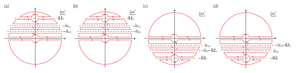
Figure 23: Contours used for the analytic continuations of the AL$1$ term in (a) region $22$-II and (b) region $22$-III or $22$-IV and of the AL$2$ term in (c) region $22$-II or $22$-III and (d) region $22$-IV.

where we have used the contour $C$ shown in Fig. 23(a) and introduced $W^{\textrm{AL}(\textrm{RA})}_{abcd;ABCD}(q_{1};q_{2})$,

$$W^{\textrm{AL}(\textrm{RA})}_{abcd;ABCD}(q_{1};q_{2})= \dfrac{3}{2}\tilde{N}_{abcd}^{\textrm{S}(\textrm{R})}(\bm{q}_{1},\omega_{1})\tilde{N}_{ABCD}^{\textrm{S}(\textrm{A})}(\bm{q}_{2},\omega_{2})$$

$$+\dfrac{1}{2}\tilde{N}_{abcd}^{\textrm{C}(\textrm{R})}(\bm{q}_{1},\omega_{1})\tilde{N}_{ABCD}^{\textrm{C}(\textrm{A})}(\bm{q}_{2},\omega_{2})$$

$$-U_{acbd}^{\uparrow\downarrow}U_{ACBD}^{\uparrow\downarrow}.$$ (127)

Furthermore, we have not explicitly written the terms of the principal integral since those terms exactly cancel out the terms of the principal integral for region 22-III or 22-IV; due to this cancellation, such terms are unnecessary to calculate the kernel of the CVCs since part of the kernel, $\mathcal{J}_{22;cdCD}^{(1)}(k,k^{\prime};0)$, is proportional to the difference between the AL1 terms for the different regions [see Eq. (89)]. In deriving Eq. (126), we have used a relation of the single-particle Green’s function as a result of the time-reversal and the even-parity symmetry, $G_{ab}^{(\textrm{R})}(k)=G_{ab}^{(\textrm{A})}(k)^{\ast}$; as described in Sect. II C, for more general derivation, we should replace $\textrm{Im}G_{ab}^{(\textrm{R})}(k)$ by $\frac{1}{2i}[G_{ab}^{(\textrm{R})}(k)-G_{ab}^{(\textrm{A})}(k)]$. (The similar remark holding in the other cases of the AL term is not described below.) Then, in the similar way for region 22-II by using the contour $C$ shown in Fig. 23(b), we obtain the AL1 term in region 22-III or 22-IV:

$$\Gamma_{22\textrm{-III};abcd}^{(1)\textrm{AL}1}(k,k^{\prime};q)= -\frac{1}{N}\sum\limits_{\bm{q}^{\prime}}\sum\limits_{\{A\}}\int^{\infty}_{-\infty}\frac{d\omega^{\prime}}{2\pi}\tanh\frac{\omega^{\prime}+\epsilon^{\prime}}{2T}\textrm{Im}G_{CA}^{(\textrm{R})}(k^{\prime}+q^{\prime})G_{BD}^{(\textrm{R})}(k+q^{\prime})W^{\textrm{AL}(\textrm{RA})}_{aBcA;dCbD}(q-q^{\prime};-q^{\prime})$$

$$-\frac{1}{N}\sum\limits_{\bm{q}^{\prime}}\sum\limits_{\{A\}}\int^{\infty}_{-\infty}\frac{d\omega^{\prime}}{2\pi}\tanh\frac{\omega^{\prime}+\epsilon}{2T}G_{CA}^{(\textrm{A})}(k^{\prime}+q^{\prime})\textrm{Im}G_{BD}^{(\textrm{R})}(k+q^{\prime})W^{\textrm{AL}(\textrm{RA})}_{aBcA;dCbD}(q-q^{\prime};-q^{\prime})$$

$$+(\textrm{Principal integral terms}).$$ (128)

and

$$\Gamma_{22\textrm{-IV};abcd}^{(1)\textrm{AL}1}(k,k^{\prime};q)=\Gamma_{22\textrm{-III};abcd}^{(1)\textrm{AL}1}(k,k^{\prime};q).$$ (129)

Third, carrying out the analytic continuation of the AL2 term in the similar way for the AL1 term by using the contour $C$ shown in Fig. 23(c) or 23(d), we obtain the AL2 term for region 22-II or 22-III or 22-IV. Namely, the AL2 terms in regions 22-II, 22-III, and 22-IV are given by, respectively,

$$\Gamma_{22\textrm{-II};abcd}^{(1)\textrm{AL}2}(k,k^{\prime};q)= -\frac{1}{N}\sum\limits_{\bm{q}^{\prime}}\sum\limits_{\{A\}}\int^{\infty}_{-\infty}\frac{d\omega^{\prime}}{2\pi}\tanh\frac{\omega^{\prime}-\epsilon^{\prime}}{2T}[-\textrm{Im}G_{AC}^{(\textrm{R})}(k^{\prime}-q^{\prime})]G_{BD}^{(\textrm{R})}(k+q+q^{\prime})W^{\textrm{AL}(\textrm{RA})}_{aBAd;CcbD}(-q^{\prime};-q-q^{\prime})$$

$$-\frac{1}{N}\sum\limits_{\bm{q}^{\prime}}\sum\limits_{\{A\}}\int^{\infty}_{-\infty}\frac{d\omega^{\prime}}{2\pi}\tanh\frac{\omega^{\prime}+\epsilon+\omega}{2T}G_{AC}^{(\textrm{R})}(k^{\prime}-q^{\prime})\textrm{Im}G_{BD}^{(\textrm{R})}(k+q+q^{\prime})W^{\textrm{AL}(\textrm{RA})}_{aBAd;CcbD}(-q^{\prime};-q-q^{\prime})$$

$$+(\textrm{Principal integral terms}),$$ (130)

$$\Gamma_{22\textrm{-III};abcd}^{(1)\textrm{AL}2}(k,k^{\prime};q)= \Gamma_{22\textrm{-II};abcd}^{(1)\textrm{AL}2}(k,k^{\prime};q),$$ (131)

and

$$\Gamma_{22\textrm{-IV};abcd}^{(1)\textrm{AL}2}(k,k^{\prime};q)= -\frac{1}{N}\sum\limits_{\bm{q}^{\prime}}\sum\limits_{\{A\}}\int^{\infty}_{-\infty}\frac{d\omega^{\prime}}{2\pi}\tanh\frac{\omega^{\prime}-\epsilon^{\prime}}{2T}[-\textrm{Im}G_{AC}^{(\textrm{R})}(k^{\prime}-q^{\prime})]G_{BD}^{(\textrm{A})}(k+q+q^{\prime})W^{\textrm{AL}(\textrm{RA})}_{aBAd;CcbD}(-q^{\prime};-q-q^{\prime})$$

$$-\frac{1}{N}\sum\limits_{\bm{q}^{\prime}}\sum\limits_{\{A\}}\int^{\infty}_{-\infty}\frac{d\omega^{\prime}}{2\pi}\tanh\frac{\omega^{\prime}+\epsilon+\omega}{2T}G_{AC}^{(\textrm{A})}(k^{\prime}-q^{\prime})\textrm{Im}G_{BD}^{(\textrm{R})}(k+q+q^{\prime})W^{\textrm{AL}(\textrm{RA})}_{aBAd;CcbD}(-q^{\prime};-q-q^{\prime})$$

$$+(\textrm{Principal integral terms}).$$ (132)

Appendix G Technical details about numerically solving the Bethe-Salpeter equation for the current

In this appendix, I give several technical remarks about the numerical calculations to self-consistently determine the current from the Bethe-Salpeter equation.

Before the remarks about the iterative self-consistent procedures of the Bethe-Salpeter equation, I remark on how to numerically calculate the frequency integral. We calculate the frequency integral by discretizing it with finite interval such as $\Delta\epsilon_{j}$ and approximating the upper and the lower value of the integral by the finite cutoff values such as $\epsilon_{\textrm{c}}$ and $-\epsilon_{\textrm{c}}$, respectively; those values can be appropriately chosen within the numerical accuracy. (In the similar way, we numerically calculate the frequency integrals of the conductivities.)

We can self-consistently solve the Bethe-Salpeter equation for the current including the $\Sigma$ CVC, the MT CVC, and the AL CVC by iteration in the following procedures.

First, we determine the MT CVC in the presence of the $\Sigma$ CVC. Using the input of the current, which is $\Lambda_{\nu;2;AB}^{(0)}(\bm{k},\epsilon_{j};0)$ for the first iteration, we determine $\tilde{\Lambda}_{\nu;2;ab}(\bm{k},\epsilon_{j};0)$ from Eq. (74). After carrying out the Fourier transformations of $\tilde{\Lambda}_{\nu;2;CD}(\bm{k},\epsilon_{j};0)$ and $\textrm{Im}V_{cCdD}^{(\textrm{R})}(\bm{k}-\bm{k}^{\prime},\epsilon_{j}-\epsilon^{\prime}_{j^{\prime}})$ about momentum, we calculate $\Delta\Lambda_{\nu;2;cd}^{\textrm{MT}}(\bm{r},\epsilon_{j};0)$ as follows:

$$\Delta\Lambda_{\nu;2;cd}^{\textrm{MT}}(\bm{r},\epsilon_{j};0)= \sum\limits_{C,D}\sum\limits_{\epsilon_{j^{\prime}}^{\prime}}\dfrac{\Delta\epsilon_{j^{\prime}}^{\prime}}{2\pi}F_{ct}^{\textrm{MT}}(\epsilon_{j},\epsilon^{\prime}_{j^{\prime}};T)$$

$$\times\textrm{Im}V_{cCdD}^{(\textrm{R})}(\bm{r},\epsilon_{j}-\epsilon^{\prime}_{j^{\prime}})$$

$$\times\tilde{\Lambda}_{\nu;2;CD}(\bm{r},\epsilon_{j^{\prime}}^{\prime};0).$$ (133)

Since $F_{ct}^{\textrm{MT}}(\epsilon_{j},\epsilon^{\prime}_{j^{\prime}};T)$ includes the hyperbolic cotangent [see Eq. (65)] and its principal integral has the $0$/$0$ structure due to $\textrm{Im}V_{cCdD}^{(\textrm{R})}(\bm{r},0)=0$, the principal integral can be calculated as follows NA-review :

$$\sum\limits_{\epsilon_{j^{\prime}}^{\prime}}\dfrac{\Delta\epsilon_{j^{\prime}}^{\prime}}{2\pi}\coth\frac{\epsilon_{j}-\epsilon_{j^{\prime}}^{\prime}}{2T}\textrm{Im}V_{cCdD}^{(\textrm{R})}(\bm{r},\epsilon_{j}-\epsilon^{\prime}_{j^{\prime}})$$

$$\times\tilde{\Lambda}_{\nu;2;CD}(\bm{r},\epsilon^{\prime}_{j^{\prime}};0)$$

$$= \sum\limits_{\epsilon_{j^{\prime}}^{\prime}\neq\epsilon_{j}}\dfrac{\Delta\epsilon_{j^{\prime}}^{\prime}}{2\pi}\coth\frac{\epsilon_{j}-\epsilon_{j^{\prime}}^{\prime}}{2T}\textrm{Im}V_{cCdD}^{(\textrm{R})}(\bm{r},\epsilon_{j}-\epsilon^{\prime}_{j^{\prime}})$$

$$\times\tilde{\Lambda}_{\nu;2;CD}(\bm{r},\epsilon^{\prime}_{j^{\prime}};0)$$

$$-\dfrac{\Delta\epsilon_{j^{\prime}}^{\prime}}{2\pi}T\dfrac{\partial}{\partial\epsilon^{\prime}_{j^{\prime}}}\bigl{[}(e^{\frac{\epsilon^{\prime}_{j^{\prime}}-\epsilon_{j}}{T}}+1)\textrm{Im}V_{cCdD}^{(\textrm{R})}(\bm{r},\epsilon_{j}-\epsilon^{\prime}_{j^{\prime}})$$

$$\ \ \ \ \ \ \ \ \ \ \ \ \ \ \ \ \ \ \ \ \ \ \ \ \times\tilde{\Lambda}_{\nu;2;CD}(\bm{r},\epsilon^{\prime}_{j^{\prime}};0)\bigr{]}\Bigl{|}_{\epsilon^{\prime}_{j^{\prime}}=\epsilon_{j}}.$$ (134)

After the Fourier transformation of $\Delta\Lambda_{\nu;2;cd}^{\textrm{MT}}(\bm{r},\epsilon_{j};0)$ about $\bm{r}$, we obtain the MT CVC, $\Delta\Lambda_{\nu;2;cd}^{\textrm{MT}}(\bm{k},\epsilon_{j};0)$, and then add this to the input of the current. (If we consider only the MT CVC, i.e. neglect the AL CVC, we skip the following second and third steps, and the sum of the input and the MT CVC becomes the output.)

Second, we turn to the calculation of the AL1 CVC. Carrying out the Fourier transformation of $\textrm{Im}G_{cc}^{(\textrm{R})}(\bm{k},\epsilon_{j^{\prime}}^{\prime})$ about $\bm{k}$ and using $\tilde{\Lambda}_{\nu;2;cc}(\bm{r},\epsilon_{j};0)$, which is the same for the calculation of the MT CVC, we calculate $\bigl{[}\textrm{Im}G\tilde{\Lambda}\bigr{]}_{c}(-\bm{k};\epsilon_{j^{\prime}}^{\prime},\omega^{\prime}_{j^{\prime\prime}})$ from the equation,

$$\bigl{[}\textrm{Im}G\tilde{\Lambda}\bigr{]}_{c}(-\bm{k};\epsilon_{j^{\prime}}^{\prime},\omega^{\prime}_{j^{\prime\prime}})= \sum\limits_{\bm{r}}e^{i\bm{k}\cdot\bm{r}}\textrm{Im}G_{cc}^{(\textrm{R})}(\bm{r},\epsilon^{\prime}_{j^{\prime}}+\omega^{\prime}_{j^{\prime\prime}})$$

$$\times\tilde{\Lambda}_{\nu;2;cc}(-\bm{r},\epsilon_{j^{\prime}}^{\prime};0).$$ (135)

After calculating $\tilde{N}_{cccc}^{\textrm{S}(\textrm{R})}(\bm{q},\omega_{j})$ and $\tilde{N}_{cccc}^{\textrm{C}(\textrm{R})}(\bm{q},\omega_{j})$ from Eqs. (78) and (79), respectively, and using Eq. (77), we determine $X_{c}^{\textrm{AL}1}(\bm{k};\epsilon_{j},\omega_{j^{\prime\prime}}^{\prime})$ from the following equation:

$$X_{c}^{\textrm{AL}1}(\bm{k};\epsilon_{j},\omega_{j^{\prime\prime}}^{\prime})= \sum\limits_{\epsilon_{j^{\prime}}^{\prime}}\Delta\epsilon_{j^{\prime}}^{\prime}F_{\textrm{tt}}^{\textrm{AL}1}(\epsilon_{j},\epsilon^{\prime}_{j^{\prime}},\omega^{\prime}_{j^{\prime\prime}};T)$$

$$\times F_{\textrm{ct}}^{\textrm{AL}1}(\epsilon_{j},\epsilon^{\prime}_{j^{\prime}};T)W_{c}^{\textrm{AL}(\textrm{RA})}(\bm{k},-\omega_{j^{\prime\prime}}^{\prime})$$

$$\times\bigl{[}\textrm{Im}G\tilde{\Lambda}\bigr{]}_{c}(-\bm{k};\epsilon_{j^{\prime}}^{\prime},\omega^{\prime}_{j^{\prime\prime}}).$$ (136)

In the above equation, we can calculate the principal integral of the hyperbolic cotangent of $F_{\textrm{ct}}^{\textrm{AL}1}(\epsilon_{j},\epsilon^{\prime}_{j^{\prime}};T)$ in the similar way for the MT CVC since that principal integral also has the $0$/$0$ structure due to $F_{\textrm{tt}}^{\textrm{AL}1}(\epsilon_{j},\epsilon_{j},\omega^{\prime}_{j^{\prime\prime}};T)=0$ [see Eq. (67)]. Carrying out the Fourier transformation of $X_{c}^{\textrm{AL}1}(\bm{k};\epsilon_{j},\omega_{j^{\prime\prime}}^{\prime})$ about $\bm{k}$ and using the equation,

$$\Delta\Lambda_{\nu;2;cc}^{\textrm{AL}1}(\bm{k},\epsilon_{j};0)= -\frac{1}{4\pi^{2}}\sum\limits_{\bm{r}}e^{-i\bm{k}\cdot\bm{r}}\sum\limits_{\omega_{j^{\prime\prime}}^{\prime}}\Delta\omega_{j^{\prime\prime}}^{\prime}$$

$$\times\textrm{Im}G_{cc}^{(\textrm{R})}(\bm{r},\epsilon_{j}+\omega^{\prime}_{j^{\prime\prime}})$$

$$\times X_{c}^{\textrm{AL}1}(\bm{r};\epsilon_{j},\omega_{j^{\prime\prime}}^{\prime}),$$ (137)

we obtain the AL1 CVC, $\Delta\Lambda_{\nu;2;cc}^{\textrm{AL}1}(\bm{k},\epsilon_{j};0)$. At this point, we add the AL1 CVC to the sum of the input of the current and the MT CVC.

Third, we calculate the AL2 CVC. Using $\bigl{[}\textrm{Im}G\tilde{\Lambda}\bigr{]}_{c}(\bm{k};\epsilon_{j^{\prime}}^{\prime},-\omega^{\prime}_{j^{\prime\prime}})$ and $W_{c}^{\textrm{AL}(\textrm{RA})}(\bm{k},-\omega_{j^{\prime\prime}}^{\prime})$ (which have been determined in the above second step), we calculate $X_{c}^{\textrm{AL}2}(\bm{k};\epsilon_{j},\omega_{j^{\prime\prime}}^{\prime})$ from the following equation:

$$X_{c}^{\textrm{AL}2}(\bm{k};\epsilon_{j},\omega_{j^{\prime\prime}}^{\prime})= \sum\limits_{\epsilon_{j^{\prime}}^{\prime}}\Delta\epsilon_{j^{\prime}}^{\prime}F_{\textrm{tt}}^{\textrm{AL}2}(\epsilon_{j},\epsilon^{\prime}_{j^{\prime}},\omega^{\prime}_{j^{\prime\prime}};T)$$

$$\times F_{\textrm{ct}}^{\textrm{AL}2}(\epsilon_{j},\epsilon^{\prime}_{j^{\prime}};T)W_{c}^{\textrm{AL}(\textrm{RA})}(\bm{k},-\omega_{j^{\prime\prime}}^{\prime})$$

$$\times\bigl{[}\textrm{Im}G\tilde{\Lambda}\bigr{]}_{c}(\bm{k};\epsilon_{j^{\prime}}^{\prime},-\omega^{\prime}_{j^{\prime\prime}}).$$ (138)

Since $F_{\textrm{tt}}^{\textrm{AL}2}(\epsilon_{j},-\epsilon_{j},\omega^{\prime}_{j^{\prime\prime}};T)=0$ is satisfied in the above equation [see Eq. (69)], we can calculate the principal integral of the hyperbolic cotangent of $F_{\textrm{ct}}^{\textrm{AL}2}(\epsilon_{j},\epsilon^{\prime}_{j^{\prime}};T)$ in the similar way for the MT CVC. After the Fourier transformation of $X_{c}^{\textrm{AL}2}(\bm{k};\epsilon_{j},\omega_{j^{\prime\prime}}^{\prime})$ about $\bm{k}$, we obtain the AL2 CVC, $\Delta\Lambda_{\nu;2;cc}^{\textrm{AL}2}(\bm{k},\epsilon_{j};0)$:

$$\Delta\Lambda_{\nu;2;cc}^{\textrm{AL}2}(\bm{k},\epsilon_{j};0)= -\frac{1}{4\pi^{2}}\sum\limits_{\bm{r}}e^{-i\bm{k}\cdot\bm{r}}\sum\limits_{\omega_{j^{\prime\prime}}^{\prime}}\Delta\omega_{j^{\prime\prime}}^{\prime}$$

$$\times\textrm{Im}G_{cc}^{(\textrm{R})}(\bm{r},\epsilon_{j}+\omega_{j^{\prime\prime}}^{\prime})$$

$$\times X_{c}^{\textrm{AL}2}(\bm{r};\epsilon_{j},\omega_{j^{\prime\prime}}^{\prime}).$$ (139)

Adding the AL2 CVC to the sum of the input of the current, the MT CVC, and the AL1 CVC, we obtain the output of the current for the Bethe-Salpeter equation with the $\Sigma$ CVC, the MT CVC, and the AL CVC.

Finally, estimating the sum of the difference between the absolute values of the output and the input of the current, we judge whether the output can be regarded as the solution of the Bethe-Salpeter equation within the numerical accuracy: if the difference becomes less than $10^{-4}$, the solution is assumed to be obtained; otherwise, after replacing the input by the output, we solve the above procedures again.

Appendix H Method to determine the dominant fluctuations in a multiorbital Hubbard model

In this appendix, I explain how to determine the dominant fluctuations in a multiorbital Hubbard model among the four kinds of fluctuations.

To discuss the dominant fluctuations in a multiorbital Hubbard model, we need to consider charge fluctuations, spin fluctuations, orbital fluctuations, and spin-orbital-combined fluctuations Ueda-paramag . This is because the Hubbard interaction terms can be expressed in terms of their operators Ueda-paramag . Then, spin and spin-orbital-combined fluctuations are described by $\chi_{abcd}^{\textrm{S}}(\bm{q},i\Omega_{n})$, and charge and orbital fluctuations are described by $\chi_{abcd}^{\textrm{C}}(\bm{q},i\Omega_{n})$ Ueda-paramag ; NA-paramag . For example, spin fluctuations are characterized by $\chi^{\textrm{S}}(\bm{q},i\Omega_{n})=\sum_{a,b}\chi^{\textrm{S}}_{aabb}(\bm{q},i\Omega_{n})$ Ueda-paramag ; NA-paramag ; spin-orbital-combined fluctuations are characterized by the correlation function between the products of the spin and the orbital operator, e.g. $\sum_{a}[\chi^{\textrm{S}}_{aa32}(\bm{q},i\Omega_{n})+\chi^{\textrm{S}}_{aa23}(\bm{q},i\Omega_{n})]$ Ueda-paramag ; NA-paramag .

Since those four kinds of fluctuations have the different dependence on $J_{\textrm{H}}$ or $U$, the dominant fluctuations can be determined by analyzing $J_{\textrm{H}}$ and $U$ dependences of $\lambda^{\textrm{S}}_{\textrm{max}}(\bm{q})^{-1}$ and $\lambda^{\textrm{C}}_{\textrm{max}}(\bm{q})^{-1}$. The difference in the $J_{\textrm{H}}$ or $U$ dependence arises from the difference in the dependence of the bare four-point vertex function characterizing the fluctuation. For example, in case NA-paramag of a $t_{2g}$-orbital Hubbard model with $J^{\prime}=J_{\textrm{H}}$ and $U^{\prime}=U-2J_{\textrm{H}}$, the bare four-point vertex function for charge fluctuations is $-U-4U^{\prime}+2J_{\textrm{H}}=-5U+10J_{\textrm{H}}$; that for spin fluctuations is $U+2J_{\textrm{H}}$; that for orbital fluctuations is $U^{\prime}-2J_{\textrm{H}}-J^{\prime}=U-5J_{\textrm{H}}$ or $U^{\prime}-2J_{\textrm{H}}+J^{\prime}=U-3J_{\textrm{H}}$ or $-U+2U^{\prime}-J_{\textrm{H}}=U-5J_{\textrm{H}}$; that for orbital-spin-combined fluctuations is $U^{\prime}+J^{\prime}=U-J_{\textrm{H}}$ or $U^{\prime}-J^{\prime}=U-3J_{\textrm{H}}$ or $U-J_{\textrm{H}}$. Thus, if orbital or spin-orbital-combined fluctuations are dominant, we obtain non-monotonic $J_{\textrm{H}}$ dependence of $\lambda^{\textrm{C}}_{\textrm{max}}(\bm{q})^{-1}$ or $\lambda^{\textrm{S}}_{\textrm{max}}(\bm{q})^{-1}$, respectively, with increasing $J_{\textrm{H}}$ since the bare four-point vertex function characterizing those fluctuations changes from repulsive to attractive at a critical value of $J_{\textrm{H}}$ as a function of $U$; if spin fluctuations are dominant, we obtain monotonic $J_{\textrm{H}}$ dependence of $\lambda^{\textrm{S}}_{\textrm{max}}(\bm{q})^{-1}$ with increasing $J_{\textrm{H}}$ due to the always repulsive bare four-point vertex function characterizing those. Note that charge fluctuations are always suppressed in a realistic set of the Hubbard interaction terms.

- (1) P. Fazekas, Lecture Notes on Electron Correlation and Magnetism (World Scientific, Singapore, 1999).
- (2) T. Moriya, J. Magn. Magn. Mater. 14, 1, (1979).
- (3) H. Kontani, Rep. Prog. Phys. 71, 026501, (2008).
- (4) M. Imada, A. Fujimori, and Y. Tokura, Rev. Mod. Phys. 70, 1039, (1998).
- (5) N. W. Ashcroft and N. D. Mermin, Solid State Physics (Thomson Learning, Ithaca, 1976).
- (6) J. M. Ziman, Principles of the Theory of Solids (Cambridge University Press, Cambridge, 1979).
- (7) L. D. Landau, ZhETF 30, 1058 (1956) [Sov. Phys. JETP 3, 920 (1957)].
- (8) P. Nozires, Theory of Interacting Fermi Systems (Westview Press, Colorado, 1997).
- (9) A. A. Abrikosov, L. P. Gor’kov, I. E. Dyaloshinski, Methods of Quantum Field Theory in Statistical Physics (Dover Publications, Mineola, 1963).
- (10) N. Arakawa, Mod. Phys. Lett. B 29, 1530005, (2015).
- (11) Y. Maeno, K. Yoshida, H. Hashimoto, S. Nishizaki, S. Ikeda, M. Nohara, T. Fujita, A. P. Mackenzie, N. E. Hussey, J. G. Bednorz, and F. Lichtenberg, J. Phys. Soc. Jpn. 66, 1405 (1997).
- (12) N. E. Hussey, A. P. Mackenzie, J. R. Cooper, Y. Maeno, S. Nishizaki, and T. Fujita, Phys. Rev. B 57, 5505 (1998).
- (13) A. P. Mackenzie, S. R. Julian, A. J. Diver, G. J. McMullan, M. P. Ray, G. G. Lonzarich, Y. Maeno, S. Nishizaki, and T. Fujita, Phys. Rev. Lett. 76, 3786 (1996).
- (14) A. P. Mackenzie and Y. Maeno, Rev. Mod. Phys. 75, 657 (2003).
- (15) K. Yamada and Y. Yosida, Prog. Theor. Phys. 76, 621 (1986).
- (16) M. Minakata and Y. Maeno, Phys. Rev. B 63, 180504(R) (2001).
- (17) N. Kikugawa and Y. Maeno, Phys. Rev. Lett. 89, 117001 (2002).
- (18) S. Nakatsuji and Y. Maeno, Phys. Rev. Lett. 84, 2666 (2000).
- (19) L. M. Galvin, R. S. Perry, A. W. Tyler, A. P. Mackenzie, S. Nakatsuji, and Y. Maeno, Phys. Rev. B 63, 161102(R) (2001).
- (20) M. Braden, O. Friedt, Y. Sidis, P. Bourges, M. Minakata, and Y. Maeno, Phys. Rev. Lett. 88, 197002 (2002).
- (21) Y. Sidis, M. Braden, P. Bourges, B. Hennion, S. NishiZaki, Y. Maeno, and Y. Mori, Phys. Rev. Lett. 83, 3320 (1999).
- (22) O. Friedt, M. Braden, G. Andr, P. Adelmann, S. Nakatsuji, and Y. Maeno, Phys. Rev. B 63, 174432 (2001).
- (23) Z. Fang and K. Terakura, Phys. Rev. B 64, 020509(R) (2001).
- (24) N. Arakawa and M. Ogata, Phys. Rev. B 86, 125126 (2012).
- (25) H.-J. Noh, S.-J. Oh, B.-G. Park, J.-H. Park, J.-Y. Kim, H.-D. Kim, T. Mizokawa, L. H. Tjeng, H.-J. Lin, C. T. Chen, S. Schuppler, S. Nakatsuji, H. Fukazawa, and Y. Maeno, Phys. Rev. B 72, 052411 (2005).
- (26) T. Oguchi, Phys. Rev. B 51, 1385 (1995).
- (27) I. I. Mazin and D. J. Singh, Phys. Rev. Lett. 79, 733 (1997).
- (28) A. Damascelli, D. H. Lu, K. M. Shen, N. P. Armitage, F. Ronning, D. L. Feng, C. Kim, Z.-X. Shen, T. Kimura, Y. Tokura, Z. Q. Mao, and Y. Maeno, Phys. Rev. Lett. 85, 5194 (2000).
- (29) Y. Yanase, T. Jujo, T. Nomura, H. Ikeda, T. Hotta, and K. Yamada, Physics Reports 387, 1 (2003).
- (30) N. E. Bickers, D. J. Scalapino, and S. R. White, Phys. Rev. Lett. 62, 961 (1989).
- (31) N. E. Bickers and D. J. Scalapino, Annals of Physics 193, 206 (1989).
- (32) N. E. Bickers and S. R. White, Phys. Rev. B 43, 8044 (1991).
- (33) T. Takimoto, T. Hotta, and K. Ueda, Phys. Rev. B 69, 104504 (2004).
- (34) H. Ikeda, R. Arita, and J. Kuneš, Phys. Rev. B 81, 054502 (2010).
- (35) K. Maki, Prog. Theor. Phys. 40, 193 (1968).
- (36) R. S. Thompson, Phys. Rev. B 1, 327 (1970).
- (37) H. Kontani, K. Kanki, and K. Ueda, Phys. Rev. B 59, 14723 (1999).
- (38) N. Arakawa, Phys. Rev. B 90, 245103 (2014).
- (39) S. Ohsugi, Y. Kitaoka, K. Ishida, and K. Asayama, J. Phys. Soc. Jpn. 60, 2351 (1991).
- (40) S. W. Tozer, A. W. Kleinsasser, T. Penney, D. Kaiser, and F. Holtzberg, Phys. Rev. Lett. 59, 1768 (1987).
- (41) T. Penney, S. von Molnár, D. Kaiser, F. Holtzberg, and A. W. Kleinsasser, Phys. Rev. B 38, 2918 (1988).
- (42) A. P. Mackenzie, N. E. Hussey, A. J. Diver, S. R. Julian, Y. Maeno, S. Nishizaki, and T. Fujita, Phys. Rev. B 54, 7425 (1996).
- (43) N. Kikugawa, A. P. Mackenzie, C. Bergemann, and Y. Maeno, Phys. Rev. B 70, 174501 (2004).
- (44) L. G. Aslamasov and A. I. Larkin, Fizika tvervd. tela, 10 (4), 1104 (1968) [Sov. Phys. Solid State 10, 875 (1968)].
- (45) S. Wermbter and L. Tewordt, Physica C 199, 375 (1992).
- (46) G. M. liashberg, ZhETF 41, 1241 (1962) [Sov. Phys. JETP 14, 886 (1962)].
- (47) H. Fukuyama, H. Ebisawa, and Y. Wada, Prog. Theor. Phys. 42, 494 (1969).
- (48) H. Kohno and K. Yamada, Prog. Theor. Phys. 80, 623 (1988).
- (49) T. Oguchi, J. Phys. Soc. Jpn. 78, 044702 (2009).
- (50) K. Yamada, Electron Correlation in Metals (Cambridge University Press, Cambridge, 2004).
- (51) R. Kubo, J. Phys. Soc. Jpn. 12, 570 (1957).
- (52) L. Onsager, Phys. Rev. 37, 405 (1931).
- (53) L. Onsager, Phys. Rev. 38, 2265 (1931).
- (54) T. Konno, Busshitsu no taishousei to gunron [in Japanese] (Kyoritsu shuppan, Tokyo, 2001).
- (55) J. M. Luttinger and J. C. Ward, Phys. Rev. 118, 1417 (1960).
- (56) G. Baym and L. P. Kadanoff, Phys. Rev. 124, 287 (1961).
- (57) W. Xu, K. Haule, and G. Kotliar, Phys. Rev. Lett. 111, 036401 (2013).
- (58) E. Kozik, M. Ferrero, and A. Georges, Phys. Rev. Lett. 114, 156402 (2015).
- (59) R. Eder, arXiv:1407.6599.
- (60) C. Hori, Ph.D. thesis [in Japanese], The University of Tokyo (2011).
- (61) H. J. Vildberg and J. W. Serene, J. Low Temp. Phys. 29, 179 (1977).
- (62) H. Kusunose, unpublished.
- (63) H. Tsunetsugu, J. Phys. Soc. Jpn. 71, 1844 (2002).
- (64) N. Arakawa and M. Ogata, Phys. Rev. B 87, 195110 (2013).
- (65) Y. Yamashita and K. Ueda, Phys. Rev. B 67, 195107 (2003).
- (66) N. Arakawa, unpublished; I adopted the method of Ref. Ueda-paramag, to a -orbital Hubbard model including not only the , , and terms but also the term, which was neglected in Ref. Ueda-paramag, .
- (67) S. Koikegami, S. Fujimoto, and K. Yamada, J. Phys. Soc. Jpn. 66, 1438 (1997).
- (68) R. Hlubina and T. M. Rice, Phys. Rev. B 51, 9253 (1995).
- (69) K. Ishida, H. Mukuda, Y. Minami, Y. Kitaoka, Z. Q. Mao, H. Fukazawa, and Y. Maeno, Phys. Rev. B 64, 100501(R) (2001).
- (70) K. Ishida, Y. Minami, Y. Kitaoka, S. Nakatsuji, N. Kikugawa, and Y. Maeno, Phys. Rev. B 67, 214412 (2003).
- (71) Y. Yanase and M. Ogata, J. Phys. Soc. Jpn. 72, 673 (2003).
- (72) H. Ikeda, J. Phys. Soc. Jpn. 77, 123707 (2008).
- (73) H. Kontani and K. Yamada, J. Phys. Soc. Jpn. 63, 2627 (1994).
- (74) J. Mravlje, M. Aichhorn, T. Miyake, K. Haule, G. Kotliar, and A. Georges, Phys. Rev. Lett. 106, 096401 (2011).
- (75) J. Mravlje and A. Georges, arXiv:1504.03860.
- (76) C. Noce and M. Cuoco, Phys. Rev. B 62, 9884 (2000).
- (77) W. Metzner and D. Vollhardt, Phys. Rev. Lett. 62, 324 (1989).
- (78) A. Georges, G. Kotliar, W. Krauth, and M. J. Rozenberg, Rev. Mod. Phys. 68, 13 (1996).
- (79) G. Kotliar, S. Y. Savrasov, K. Haule, V. S. Oudovenko, O. Parcollet, and C. A. Marianetti, Rev. Mod. Phys. 78, 865 (2006).
- (80) O. Parcollet, G. Biroli, and G. Kotliar, Phys. Rev. Lett. 92, 226402 (2004).
- (81) Y. Nomura, S. Sakai, and R. Arita, Phys. Rev. B 89, 195146 (2014).
- (82) A. Khurana, Phys. Rev. Lett. 64, 1990 (1990).
- (83) Th. Pruschke, D. L. Cox, and M. Jarrell, Phys. Rev. B 47, 3553 (1993).
- (84) P. Morel and P. Nozires, Phys. Rev. 126, 1909 (1962).
- (85) L. Klein, L. Antognazza, T. H. Geballe, M. R. Beasley, and A. Kapitulnik, Phys. Rev. B 60, 1448 (1999).
- (86) K. Izawa, H. Takahashi, H. Yamaguchi, Y. Matsuda, M. Suzuki, T. Sasaki, T. Fukase, Y. Yoshida, R. Settai, and Y. Onuki, Phys. Rev. Lett. 86, 2653 (2001).
- (87) J. Xia, Y. Maeno, P. T. Beyersdorf, M. M. Fejer, and A. Kapitulnik, Phys. Rev. Lett. 97, 167002 (2006).
- (88) Y. Nakajima, H. Shishido, H. Nakai, T. Shibauchi, K. Behnia, K. Izawa, M. Hedo, Y. Uwatoko, T. Matsumoto, R. Settai, Y. Ōnuki, H. Kontani, and Y. Matsuda, J. Phys. Soc. Jpn. 76, 024703 (2007).
- (89) G. R. Stewart, Z. Fisk, J. O. Willis, and J. L. Smith, Phys. Rev. Lett. 52, 679 (1984).
- (90) M. Dressel, J. Phys.: Condens. Matter 23, 293201 (2011).
- (91) Y. Takada, Tataimondai tokuron [in Japanese] (Asakura shoten, Tokyo, 2009).
- (92) W. H. Press, S. A. Teukolsky, W. T. Vetterling, and B. P. Flannery, NUMERICAL RECIPES in C (Cambridge University Press, Cambridge, 1988).
- (93) Y. Takada, Tataimondai [in Japanese] (Asakura shoten, Tokyo, 1999).