Quasiconformal non-parametrizability of almost smooth spheres

Abstract.

We show that, for each $n\geq 3$, there exists a smooth Riemannian metric $g$ on a punctured sphere $\mathbb{S}^{n}\setminus\{x_{0}\}$ for which the associated length metric extends to a length metric $d$ of $\mathbb{S}^{n}$ with the following properties: the metric sphere $(\mathbb{S}^{n},d)$ is Ahlfors $n$-regular and linearly locally contractible but there is no quasiconformal homeomorphism between $(\mathbb{S}^{n},d)$ and the standard Euclidean sphere $\mathbb{S}^{n}$.

1. Introduction

The (quasi)conformal gauge of the Euclidean $n$-sphere $\mathbb{S}^{n}$ is the maximal collection of all metrics $d$ on $\mathbb{S}^{n}$ for which there exists a quasiconformal homeomorphism $(\mathbb{S}^{n},d)\to\mathbb{S}^{n}$. Here, and in what follows, $\mathbb{S}^{n}$ refers to both the subset $\{(x_{1},\ldots,x_{n+1})\in\mathbb{R}^{n+1}\colon x_{1}^{2}+\cdots+x_{n+1}^{2}=1\}$ of $\mathbb{R}^{n+1}$ but also the metric space $(\mathbb{S}^{n},d_{0})$, where $d_{0}$ is the Euclidean metric induced from $\mathbb{R}^{n+1}$ by inclusion.

The problem of characterizing this gauge is a relaxation of the Beltrami problem in the analytic theory of quasiconformal mappings. Indeed, whereas the Beltrami problem asks whether a given measurable Riemannian metric $g$ on $\mathbb{S}^{n}$ admits conformal map $(\mathbb{S}^{n},g)\to(\mathbb{S}^{n},g_{0})$ into the standard Riemannian metric $g_{0}$, the gauge characterization problem merely asks for a quasiconformal map between metrics. We refer to Heinonen [11, Section 15] for a detailed discussion on the terminology and background of the (quasi)conformal gauge.

Characterization of the quasiconformal gauge has turned out to be a formidable problem, and the question remains open also for the quasisymmetric gauge in higher dimensions; the quasisymmetric gauge of the Euclidean sphere $\mathbb{S}^{n}$ consists of all metric spheres $(\mathbb{S}^{n},d)$ admitting a quasisymmetric homeomorphism $(\mathbb{S}^{n},d)\to\mathbb{S}^{n}$; see Section 2 for terminology.

In dimensions $n=1$ and $n=2$ the quasisymmetric gauge is fully understood. For $\mathbb{S}^{1}$ the metric characterization for the quasisymmetric gauge is due to Tukia and Väisälä [20] and for $\mathbb{S}^{2}$ this gauge is characterized by Bonk and Kleiner [5]; see also Wildrick [21, 22]. In particular, all Ahlfors $2$-regular and linearly locally contractible (LLC) metric $2$-spheres $(\mathbb{S}^{2},d)$ are quasisymmetrically equivalent to $\mathbb{S}^{2}$. We note in passing that Ahlfors $n$-regular and LLC metric spheres $(\mathbb{S}^{n},d)$ are $n$-Loewner spaces and quasiconformal maps $(\mathbb{S}^{n},d)\to\mathbb{S}^{n}$ are quasisymmetric; see Heinonen-Koskela [12]. We refer to Rajala [16] for recent results on quasiconformal parametrization of metric $2$-spheres.

In higher dimensions these metric conditions are not sufficient for quasisymmetric parametrization. By results of Semmes [18] (dimension $n=3$) and Heinonen–Wu [13] (dimensions $n>3$), there exists for each $n\geq 3$ an Ahlfors $n$-regular, LLC, and geodesic $n$-sphere, which is not quasisymmetrically equivalent to the standard sphere $\mathbb{S}^{n}$.

The metric sphere $(\mathbb{S}^{3},d_{S})$ Semmes considered in [18] is the decomposition space $\mathbb{S}^{3}/\mathrm{Bd}$ associated to the Bing double and the metric $d_{S}$ is obtained by an embedding $\mathbb{S}^{3}/\mathrm{Bd}\to\mathbb{S}^{4}$; see Section 2.2 for definitions. Heinonen and Wu consider in [13] the decomposition space $\mathbb{R}^{3}/\mathrm{Wh}$, associated to the Whitehead continuum, and construct an Ahlfors $3$-regular and linearly locally contractible metric $d_{\mathrm{HW}}$ on $\mathbb{R}^{3}/\mathrm{Wh}$. For $n>3$, the stabilization $\mathbb{R}^{3}/\mathrm{Wh}\times\mathbb{R}^{n-3}$ is homeomorphic to $\mathbb{R}^{n}$ and a product metric, also denoted by $d_{\mathrm{HW}}$, in the stabilized space $\mathbb{R}^{3}/\mathrm{Wh}\times\mathbb{R}^{n-3}$ is Ahlfors $n$-regular and LLC. A metric sphere $(S_{\mathrm{HW}}^{n},d_{\mathrm{HW}})$, which is not in the quasisymmetric gauge of $\mathbb{S}^{n}$, is now obtained by one-point compactification of $(\mathbb{R}^{3}/\mathrm{Wh}\times\mathbb{R}^{n-3},d_{\mathrm{HW}})$.

Neither the sphere $\mathbb{S}^{3}/\mathrm{Bd}$ nor the spheres $S_{\mathrm{HW}}^{n}$ have a priori smooth structures; choices of homeomorphisms $\mathbb{S}^{3}/\mathrm{Bd}\to\mathbb{S}^{3}$ and $S_{\mathrm{HW}}^{n}\to\mathbb{S}^{n}$ introduce such on these spaces. Note that there exists a homeomorphism $\mathbb{S}^{3}/\mathrm{Bd}\to\mathbb{S}^{3}$ and a Cantor set $C\subset\mathbb{S}^{3}/\mathrm{Bd}$ for which the domain $(\mathbb{S}^{3}/\mathrm{Bd})\setminus C$ is diffeomorphic to a domain in the standard sphere $\mathbb{S}^{3}$. Under this parametrization of $\mathbb{S}^{3}/\mathrm{Bd}$, we may take the metric $d_{S}$ to be the completion of a Riemannian distance in $(\mathbb{S}^{3}/\mathrm{Bd})\setminus C$; see Section 3 for details. Similarly, in the Heinonen–Wu example $(S_{\mathrm{HW}}^{n},d_{\mathrm{HW}})$ there exists a codimension $3$ sphere $S$ for which $S_{\mathrm{HW}}^{n}\setminus S$ is diffeomorphic to an open subset of $\mathbb{S}^{n}$ and for which $d_{HW}$ is a completion of the distance $d_{g}$ associated to a Riemannian metric $g$ in $S_{\mathrm{HW}}^{n}\setminus S$.

We say that a length metric $d$ on $\mathbb{S}^{n}$ is almost smooth if there exists a compact set $E\subset\mathbb{S}^{n}$ (called singular set) and a smooth Riemannian metric $g$ in $\mathbb{S}^{n}\setminus E$ for which $d$ is the completion of the distance $d_{g}$ associated to $g$. Recall that a metric $d$ on $\mathbb{S}^{n}$ is a length metric if $d(x,y)=\inf_{\gamma}\ell_{d}(\gamma)$ for all points $x,y\in\mathbb{S}^{n}$, where $\gamma$ is a path connecting $x$ and $y$ and $\ell_{d}(\gamma)$ is the length of $\gamma$ in metric $d$.

We show that, for each $n\geq 3$, there exists an almost smooth metric $d$ on $\mathbb{S}^{n}$ having a singular set consisting of only one point but for which there is no quasisymmetric homeomorphism $(\mathbb{S}^{n},d)\to\mathbb{S}^{n}$.

Theorem 1.1.

For each $n\geq 3$ there exists an almost smooth Ahlfors $n$-regular and linearly locally contractible length metric $d$ in $\mathbb{S}^{n}$ with a singular set consisting of a single point $x_{0}\in\mathbb{S}^{n}$ for which there is no quasiconformal homeomorphism $(\mathbb{S}^{n},d)\to\mathbb{S}^{n}$.

It should be noted that, although the singular set of the metric $d$ consists only of one point $x_{0}\in\mathbb{S}^{n}$, the quasiconformal non-parametrization of the sphere $(\mathbb{S}^{n},d)$ stems from the degeneration of the underlying Riemannian metric. Indeed, the metric $d$ we construct for Theorem 1.1 has the property that there is no quasiconformal homeomorphism $(\mathbb{S}^{n}\setminus\{x_{0}\},d)\to\mathbb{S}^{n}\setminus\{x_{0}\}$. We refer to Balogh and Koskela [2] for removability results for quasiconformal mappings to the positive direction in the metric setting.

The construction in Theorem 1.1 is based on Blankinship’s necklace [4], a higher-dimensional analogue of Antoine’s necklace which yields a wild Cantor set in $\mathbb{S}^{n}$. In the proof of Theorem 1.1 we use a modification of this construction for two rings, which we call the Bing–Blankinship construction since it gives a generalization of Bing’s double to higher dimensions. To obtain an almost smooth sphere with one singular point, we consider a sequence of partial Bing–Blankinship constructions of arbitrary length.

The non-existence of a quasiconformal homeomorphism $(\mathbb{S}^{n},d)\to\mathbb{S}^{n}$ is based on uniform modulus estimates for certain families of $(n-2)$-tori. These modulus estimates stem from uniform area estimates which replace Semmes’s length estimates in [18]. These area estimates are obtained by homological intersection counting in the spirit of Freedman and Skora [9, Lemma 2.5]; see Proposition 4.1 and Corollary 4.2.

These modulus estimates, when applied to the decomposition space associated to the Bing–Blankinship construction, yield a sharp higher dimensional metric analog of Semmes’s non-parametrizability result [18] for metrics on $\mathbb{S}^{3}$. We discuss this result (Theorem 6.1) and its relation to the result of Heinonen and Wu in Section 6.

This article is organized as follows. In Section 3, we discuss the Bing–Blankinship decomposition space $\mathbb{S}^{n}/\mathrm{BB}$ and show that $\mathbb{S}^{n}/\mathrm{BB}$ is homeomorphic to $\mathbb{S}^{n}$. We also construct the almost smooth metric $d$ in Theorem 6.1. In Section 4 we prove Freedman–Skora intersection results for the decomposition associated to $\mathbb{S}^{n}/\mathrm{BB}$. In Section 5 we discuss modulus estimates in $(\mathbb{S}^{n},d)$ and in the Euclidean sphere $\mathbb{S}^{n}$ for families of $(n-2)$-tori associated to decomposition yielding $\mathbb{S}^{n}/\mathrm{BB}$. In Section 6 we prove Theorem 6.1 and finally Theorem 1.1 in Section 7.

Acknowledgments

We thank Jang-Mei Wu for discussions on the shrinkability of the Bing–Blankinskip necklace.

2. Preliminaries

We begin this section with a general discussion on the metric theory of quasiconformal mappings and Loewner spaces. As a second topic we recall notions from point set topology related to decomposition spaces. We finish this section with a discussion on Semmes metrics on decomposition spaces.

2.1. Loewner spaces and quasiconformal maps

A homeomorphism $f\colon X\to Y$ between metric spaces $(X,d_{X})$ and $(Y,d_{Y})$ is quasiconformal if there exists $H<\infty$ satisfying

(2.1) $$\limsup_{r\to 0}\frac{\sup_{d_{X}(x,y)\leq r}d_{Y}(f(x),f(y))}{\inf_{d_{X}(x,y)\geq r}d_{Y}(f(x),f(y))}\leq H$$

for every $x\in X$. A homeomorphism $f\colon X\to Y$ is $\eta$-quasisymmetric, where $\eta\colon[0,\infty)\to[0,\infty)$ is a homeomorphism, if

$$\frac{d_{Y}(f(x),f(y))}{d_{Y}(f(x),f(z))}\leq\eta\left(\frac{d_{X}(x,y)}{d_{X}(x,z)}\right)$$

for all triples $x,y,z\in X$ of distinct points in $X$.

The spaces we consider in this article are Ahlfors $n$-regular and linearly locally contractible. A metric measure space $(X,d,\mu)$ is Ahlfors $n$-regular if there exists a constant $C>0$ for which

$$\frac{1}{C}r^{n}\leq\mu(B_{X}(x,r))\leq Cr^{n}$$

for all open metric balls $B_{X}(x,r)=\{y\in X\colon d(x,y)<r\}$ of radius $0<r\leq\operatorname{diam}{X}$ about $x$ in $X$. We call a metric space $(X,d)$ Ahlfors $n$-regular if $(X,d,\mathcal{H}^{n})$ is $n$-regular; here and in what follows $\mathcal{H}^{n}$ is the Hausdorff $n$-measure with respect to the metric $d$. Further, $X$ is linearly locally contractible if there exists $C>0$ so that each ball $B_{X}(x,r)$ in $X$ is contractible in $B_{X}(x,Cr)$ for all $r<(\operatorname{diam}X)/C$.

Connected and orientable $n$-manifolds that are Ahlfors $n$-regular and linearly locally contractible support $(1,n)$-Poincaré inequality; see [17, Theorem B.10]. Thus, when proper, they are $n$-Loewner spaces by a result of Heinonen and Koskela [12, Theorem 5.7]. Further, a quasiconformal homeomorphism between bounded Ahlfors $n$-regular spaces ($n>1$) is quasisymmetric if the domain is a Loewner space and the target linearly locally contractible [12, Theorem 4.9].

A space $(X,d,\mu)$ is $n$-Loewner if there exists nonincreasing positive function $\phi\colon(0,\infty)\to(0,\infty)$ such that

(2.2) $$\operatorname{Mod}_{n}(\Gamma(E,F))\geq\phi(t)>0$$

whenever $E$ and $F$ are two disjoint, non-degenerate continua in $X$ and

$$t\geq\frac{\text{dist}(E,F)}{\min(\operatorname{diam}{E},\operatorname{diam}{F})}.$$

Here $\operatorname{Mod}_{n}(\Gamma(E,F))$ is the $n$-modulus of the family $\Gamma(E,F)$ of all paths connecting $E$ and $F$.

Recall that the $p$-modulus $\operatorname{Mod}_{p}(\Gamma)$, for $p\geq 1$, of a path family $\Gamma$ in $(X,d,\mu)$ is

$$\operatorname{Mod}_{p}(\Gamma)=\inf\int_{X}\rho^{p}\,\mathrm{d}\mu,$$

where the infimum is taken over all non-negative Borel functions $\rho\colon X\to[0,\infty]$ satisfying

$$\int_{\gamma}\rho\,\mathrm{d}s\geq 1$$

for all locally rectifiable paths $\gamma\in\Gamma$.

More generally, given a family $\mathcal{S}$ of $l$-manifolds (possibly with boundary) in $X$, where $l\in\{1,\ldots,n-1\}$, the $p$-modulus $\operatorname{Mod}_{p}(\mathcal{S})$ of $\mathcal{S}$ is

$$\operatorname{Mod}_{p}(\mathcal{S})=\inf\int_{X}\rho^{p}\,\mathrm{d}\mu,$$

where the infimum is taken over all non-negative Borel functions $\rho\colon X\to[0,\infty]$ satisfying

(2.3) $$\int_{S}\rho(x)\,\mathrm{d}\mathcal{H}^{l}\geq 1$$

for all $S\in\mathcal{S}$. A function $\rho$ satisfying (2.3) is called an admissible function for $\mathcal{S}$.

The proofs of Theorems 1.1 and 6.1 are based on the quasi-invariance of the $n/(n-2)$-modulus of a family of $(n-2)$-manifolds. More precisely, we consider the modulus of a family $\Sigma=\{\{x\}\times(\mathbb{S}^{1})^{n-2}\subset\mathbb{B}^{2}\times(\mathbb{S}^{1})^{n-2}\colon x\in\Omega\}$ in $\mathbb{B}^{2}\times(\mathbb{S}^{1})^{n-2}$, where $\Omega\subset\mathbb{B}^{2}$ is a neighborhood of the boundary of $\mathbb{B}^{2}$. Given a quasiconformal map $f\colon\Omega\times(\mathbb{S}^{1})^{n-2}\to U$, where $U\subset\mathbb{R}^{n}$ is a domain, we have

(2.4) $$\frac{1}{C_{0}}\operatorname{Mod}_{\frac{n}{n-2}}(\Sigma)\leq\operatorname{Mod}_{\frac{n}{n-2}}(f\Sigma)\leq C_{0}\operatorname{Mod}_{\frac{n}{n-2}}(\Sigma),$$

where $C_{0}=C_{0}(n,H)>0$ depends only on $n$ and the quasiconformality constant $H$ of $f$; see [1, Theorem 6]. The $n/(n-2)$-modulus of $\Sigma$ is conformally invariant and is therefore called the conformal modulus of $\Sigma$.

Remark 2.1.

We note, in passing, that our definition for the $p$-modulus of a family of $l$-manifolds is slightly more restrictive than the definition given in Agard [1] as we have used the Hausdorff $l$-measure in the definition of admissbile functions in place of more general $l$-dimensional measure. We also refer to Rajala [15] for a definition of modulus for more general families of geometric sets.

2.2. Decomposition spaces, initial packages, and defining sequences

We introduce now the topological notions of a decomposition space and a defining sequence which will be used throughout the article. The defining sequences we consider are induced by (Semmes’s) initial packages; see [18, Section 2] for a detailed discussion on initial packages.

A decomposition of topological space $X$ is a partition of $X$. The partitions $G$ we consider are upper semi continuous (usc), that is, elements of $G$ are closed subsets of $X$ and for each $g\in G$ and every neighborhood $U$ of $g$ in $X$ there exists a neighborhood $V$ of $g$ contained in $U$ so that every $g^{\prime}\in G$ intersecting $V$ is contained in $U$. A defining sequence $\mathcal{X}=(X_{k})_{k\geq 0}$ for the decomposition $G$ is a decreasing sequence of closed sets $X$ for which the components of $\bigcap_{k\geq 0}X_{k}$ are exactly the non-degenerated elements in $G$, that is, elements $g\in G$ which are not points.

The decomposition space $X/G$ associated to $G$ is the quotient space with the quotient topology induced by the canonical map $X\to X/G$; for usc decompositions, $X/G$ is a metrizable space. We refer to Daverman [6] for a detailed discussion on decomposition spaces.

A tuple $\mathfrak{I}=(M;\varphi_{1},\ldots,\varphi_{p})$ is a smooth initial package if $M$ is a compact manifold with boundary and each $\varphi_{i}\colon M\to M$ is a smooth embedding with the property that images $\varphi_{i}(M)$ are pair-wise disjoint. Initial packages $\mathfrak{I}=(M;\varphi_{1},\ldots,\varphi_{p})$ and $\mathfrak{I}^{\prime}=(M^{\prime};\varphi^{\prime}_{1},\ldots,\varphi^{\prime}_{p})$ are equivalent if there exists a diffeomorphism $\beta\colon M\to M^{\prime}$ for which $\varphi^{\prime}_{i}=\beta\circ\varphi_{i}\circ\beta^{-1}$; we say that diffeomorphism $\beta$ conjugates $\mathfrak{I}$ and $\mathfrak{I}^{\prime}$.

Each initial package $\mathfrak{I}=(M;\varphi_{1},\ldots,\varphi_{p})$ induces a natural tree ordered by inclusion. More precisely, let $\mathcal{W}_{p}$ be the set of all finite words in alphabet $\{1,\ldots,p\}$. For each $w=i_{1}\cdots i_{k}\in\mathcal{W}_{p}$, let $\varphi_{w}\colon M\to M$ be the embedding $\varphi_{w}:=\varphi_{i_{1}}\circ\cdots\circ\varphi_{i_{k}}$; for $w=\emptyset$, we set $\varphi_{\emptyset}=\mathrm{id}$. Then $\varphi_{w}(M)\supset\varphi_{wi}(M)$ for each $i=1,\ldots,p$ and $w\in\mathcal{W}_{p}$. We call the ordered tree $\mathcal{T}_{\mathfrak{I}}=(\varphi_{w}(M))_{w\in\mathcal{W}_{p}}$ the defining tree of $\mathfrak{I}$.

The defining sequence for $\mathfrak{I}$ is the sequence $\mathcal{X}_{\mathfrak{I}}=(\mathcal{X}_{\mathfrak{I},k})_{k\geq 0}$ where $\mathcal{X}_{\mathfrak{I},k}=\bigcup_{|w|=k}\varphi_{w}(M)$ and $|w|$ is the length of the word $w$. Note that, by construction, for each $w\in\mathcal{W}_{p}$ of length $k$, the set $\varphi_{w}(M)$ is a component of $\mathcal{X}_{\mathfrak{I},k}$. The decomposition $G_{\mathfrak{I}}$ of $M$ is the decomposition associated to the defining sequence $\mathcal{X}_{\mathfrak{I}}$. We denote the set $\bigcap_{k}\mathcal{X}_{\mathfrak{I},k}$, the singular set of the initial package $\mathfrak{I}$, by $\mathcal{S}(\mathfrak{I})$.

In forthcoming sections we consider defining sequences, which are not defining sequences for initial packages, but are topologically equivalent to such defining sequences. For this purpose, we say that $\mathcal{M}=(M_{w})_{w\in\mathcal{W}_{p}}$ is an ordered tree if $M_{wi}\subset M_{w}$ for each $w\in\mathcal{W}_{p}$ and $i=1,\ldots,p$. Ordered trees $\mathcal{M}=(M_{w})_{w\in\mathcal{W}_{p}}$ and $\mathcal{M}^{\prime}=(M^{\prime}_{w})_{w\in\mathcal{W}_{p}}$ are equivalent if there exists a homeomorphism $\theta\colon M_{\emptyset}\to M^{\prime}_{\emptyset}$ satisfying $\theta(M_{w})=M^{\prime}_{w}$ for each $w\in\mathcal{W}_{p}$. Further, we say that an ordered tree $\mathcal{M}$ is equivalent to the initial package $\mathfrak{I}$ if $\mathcal{M}$ is equivalent to the tree $\mathcal{T}_{\mathfrak{I}}$.

Convention.

Let $(M;\varphi_{1},\ldots,\varphi_{p})$ be an initial package, $E\subset M$ a set, and let $w\in\mathcal{W}_{p}$ be a word. Then $E_{w}\subset M$ is the set $E_{w}=\varphi_{w}(E)$ unless otherwise specified.

2.3. Semmes metrics

The metric $d$ on $\mathbb{S}^{n}$ in Theorem 1.1 stems from a construction of a quasi-self-similar metric on a decomposition space of $\mathbb{S}^{n}$. These metrics are introduced in [18] and called Semmes metrics in [14]. They are defined as follows.

A metric $d$ on a decomposition space $M/G_{\mathfrak{I}}$ associated to an initial package $\mathfrak{I}$ is a Semmes metric if there exists $\lambda>0$ and $L\geq 1$ for which

$$\frac{\lambda^{k}}{L}d(x,y)\leq d(\varphi_{w}(x),\varphi_{w}(y))\leq L\lambda^{k}d(x,y)$$

for each $x,y\in M/G_{\mathfrak{I}}$ and each word $w=i_{1}\cdots i_{k}$; we call the metric space $(M/G_{\mathfrak{I}},d)$ a (self-similar) Semmes space and $\lambda$ the scaling constant of the metric $d$. We refer to [14, Section 7] for Semmes metrics and Semmes spaces associated to non-self-similar decomposition spaces.

Metric spaces $(M/G_{\mathfrak{I}},d)$ are Ahlfors $n$-regular and LLC under mild conditions on the metric $d$ and the initial package $\mathfrak{I}$. We record these facts as lemmas. The proofs are minor variations of the proofs of [14, Proposition 7.8] and [14, Proposition 7.9], respectively.

Lemma 2.2.

Let $M$ be an $n$-manifold with boundary for $n\geq 3$, $\mathfrak{I}=(M;\varphi_{1},\ldots,\varphi_{p})$ an initial package, and $d$ a Semmes metric on $M/G_{\mathfrak{I}}$ with a scaling constant $\lambda\in(0,p^{-1/n})$. Then $(M/G_{\mathfrak{I}},d)$ is Ahlfors $n$-regular.

Lemma 2.3.

Let $M$ be an $n$-manifold with boundary for $n\geq 3$, $\mathfrak{I}=(M,\varphi_{1},\ldots,\varphi_{p})$ an initial package, and $d$ a Semmes metric on $M/G_{\mathfrak{I}}$. Suppose $\varphi_{wi}(M)$ contracts in $\varphi_{w}(M)$ for each $w\in\mathcal{W}_{p}$ and $i\in\{1,\ldots,p\}$. Then $(M/G_{\mathfrak{I}},d)$ is linearly locally contractible.

3. Bing–Blankinship spheres

In this section, we introduce first the construction of the Bing–Blankinship necklace which yields the decomposition space $\mathbb{S}^{n}/\mathrm{BB}$. In the construction we present in this, we combine the idea of Blankinship in [4] based on Antoine’s necklace with a contruction of Bing in [3]. We also adapt Bing’s method to show that the space $\mathbb{S}^{n}/\mathrm{BB}$ is homeomorphic to $\mathbb{S}^{n}$.

3.1. The decomposition space $\mathbb{S}^{n}/\mathrm{BB}$

Let $n\geq 3$ and $\psi\colon(\mathbb{S}^{1})^{n-2}\to(\mathbb{S}^{1})^{n-2}$ be the cyclic permutation

$$(x_{1},x_{2},\ldots,x_{n-2})\mapsto(x_{n-2},x_{1},x_{2},\ldots,x_{n-3}),$$

where we understand $\psi=\mathrm{id}$ for $n=3$. Let also $\mathfrak{I}_{B}=(\mathbb{B}^{2}\times\mathbb{S}^{1};\varphi_{1},\varphi_{2})$ be an initial package for the Bing double; see Figure 1.

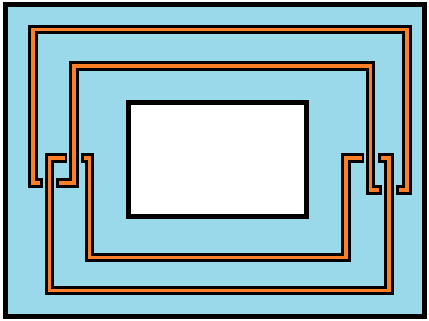
Figure 1. The Bing double.

A generalization of the initial package $\mathfrak{I}_{B}$ to dimension $n$ is

$$\mathfrak{I}_{B,n}=(\mathbb{B}^{2}\times(\mathbb{S}^{1})^{n-2};\tilde{\varphi}_{1},\tilde{\varphi}_{2}),$$

where

$$\tilde{\varphi}_{i}=(\varphi_{i}\times\mathrm{id}_{(\mathbb{S}^{1})^{n-3}})\circ(\mathrm{id}_{\mathbb{B}^{2}}\times\psi).$$

We call the initial package $\mathfrak{I}_{B,n}$ the Bing–Blankinship package; note that $\mathfrak{I}_{B,3}=\mathfrak{I}_{B}$. As in [4], we call a space homeomorphic to $\mathbb{T}=\mathbb{B}^{2}\times(\mathbb{S}^{1})^{n-2}$ an $n$-tube. We call $n$-tubes

$$\mathbb{T}_{w}=\tilde{\varphi}_{w}(\mathbb{B}^{2}\times(\mathbb{S}^{1})^{n-2})$$

for $w\in\mathcal{W}_{2}$, Blankinship rings.

To obtain a decomposition of $\mathbb{S}^{n}$, we fix a smooth embedding $\vartheta\colon\mathbb{T}\to\mathbb{S}^{n}$ for which $\vartheta(\mathbb{T})\subset\mathbb{R}^{n}\subset\mathbb{S}^{n}$ and there exists $x_{0}\in\mathbb{S}^{1}$ satisfying

• $\vartheta(\mathbb{B}^{2}\times\mathbb{S}^{1}\times\{x_{0}\}^{n-3})\subset\mathbb{R}^{3}\times\{0\}^{n-3}$,

• $\vartheta(\varphi_{i}(\mathbb{B}^{2}\times\mathbb{S}^{1})\times\{x_{0}\}^{n-3})\subset\mathbb{R}^{3}\times\{0\}^{n-3}$ for $i=1,2$, and

• $\vartheta\circ(\mathrm{id}_{\mathbb{B}^{2}}\times\psi^{k})=(\mathrm{id}_{\mathbb{R}^{2}}\times\psi^{\prime})^{k}\circ\vartheta$ for each $k\in\mathbb{N}$, where $\psi^{\prime}\colon\mathbb{R}^{n-2}\to\mathbb{R}^{n-2}$ is the cyclic permutation $(x_{1},\ldots,x_{n-2})\mapsto(x_{n-2},x_{1},\ldots,x_{n-3})$.

The decomposition space $\mathbb{S}^{n}/\mathrm{BB}$ is now the decomposition space obtained by collapsing the components of $\vartheta(\mathcal{S}(\mathfrak{I}_{B,n}))$. Thus there exists a natural embedding $\vartheta^{\prime}\colon\mathbb{T}/G_{\mathfrak{I}_{B,n}}\to\mathbb{S}^{n}/\mathrm{BB}$ satisfying

where vertical arrows are canonical maps $x\mapsto[x]$.

In the following two sections, we show that the space $\mathbb{S}^{n}/\mathrm{BB}$ admits a good embedding into the Euclidean sphere $\mathbb{S}^{n+1}$ and that $\mathbb{S}^{n}/\mathrm{BB}$ is topologically an $n$-sphere. Using this two observations, we construct in Section 3.4 an almost smooth metric on the standard $n$-sphere $\mathbb{S}^{n}$ having the Bing–Blankinship necklace as the singular set.

3.2. Embedding of $\mathbb{S}^{n}/\mathrm{BB}$ into $\mathbb{S}^{n+1}$

The space $\mathbb{S}^{n}/\mathrm{BB}$ admits a embedding into $\mathbb{S}^{n+1}$, which is modular in the terminology of [14].

Proposition 3.1.

Let $n\geq 3$ and $\lambda\in(0,1)$. Then there exists a map $\tilde{\rho}\colon\mathbb{S}^{n}\to\mathbb{S}^{n+1}$ with the following properties:

• $\tilde{\rho}|\left(\mathbb{S}^{n}\setminus\mathcal{S}(\mathfrak{I}_{B,n})\right)\colon\mathbb{S}^{n}\setminus\mathcal{S}(\mathfrak{I}_{B,n})\to\mathbb{S}^{n+1}$ is a smooth embedding for which $\tilde{\rho}(x)=x$ for every $x\in\mathbb{S}^{n}\setminus\vartheta(\mathbb{T})$, and

• there exists $L\geq 1$ so that, for each word $w\in\mathcal{W}_{2}$, the map $\tilde{\rho}_{w}=\tilde{\rho}\circ\vartheta\circ\tilde{\varphi}_{w}\circ\vartheta^{-1}|\vartheta(\mathbb{T}\setminus(\mathbb{T}_{1}\cup\mathbb{T}_{2}))\colon\vartheta(\mathbb{T}\setminus(\mathbb{T}_{1}\cup\mathbb{T}_{2}))\to\mathbb{S}^{n+1}$ satisfies

  $$\frac{\lambda^{|w|}}{L}|x-y|\leq|\tilde{\rho}_{w}(x)-\tilde{\rho}_{w}(y)|\leq L\lambda^{|w|}|x-y|$$

  for all $x,y\in\vartheta(\mathbb{T}\setminus(\mathbb{T}_{1}\cup\mathbb{T}_{2}))$.

In particular, $\tilde{\rho}(\mathcal{S}(\mathfrak{I}_{B,n}))$ is a Cantor set in $\mathbb{S}^{n+1}$ and there exists an embedding $\mathbb{S}^{n}/\mathrm{BB}\to\mathbb{S}^{n+1}$ for which the diagram

commutes.

The proof of Proposition 3.1 is a minor modification of the argument of Semmes in [18, Lemma 3.21] and we merely sketch the proof; see also [14, Section 6] for a similar construction.

Sketch of a proof of Proposition 3.1.

Let $T_{w}=\vartheta(\mathbb{T}_{w})$ for each $w\in\mathcal{W}_{2}$. Let also $\tilde{\varphi}^{\prime}_{i}=\vartheta\circ\tilde{\varphi}_{i}\circ\vartheta^{-1}|T_{\emptyset}$ for $i=1,2$. Then $\mathfrak{I}_{B,n}^{\prime}=(T_{\emptyset};\tilde{\varphi}^{\prime}_{1},\tilde{\varphi}^{\prime}_{2})$ is an initial package.

The construction of the map $\tilde{\rho}$ is self-similar with respect to the initial package $\mathfrak{I}_{B,n}^{\prime}$, and we describe only the first step. We may assume that $T=T_{\emptyset}\subset\mathbb{R}^{n}\subset\mathbb{S}^{n}$. Let $\mu=\sum_{k=0}^{\infty}\lambda^{k}$ and let $B\subset\mathbb{R}^{n}$ be a Euclidean ball containing $T$ for which $\text{dist}(T,\mathbb{R}^{n}\setminus B)\geq 2\mu$. For each $w\in\mathcal{W}_{2}$ we also denote by $C_{w}$ the cylinder $T_{w}\times[-\lambda^{|w|},\lambda^{|w|}]\subset\mathbb{R}^{n+1}$. For simplicity, we denote $C=C_{\emptyset}$ and $U=B\times[-2\mu,2\mu]$.

Let $g_{i}\colon C\to\mathbb{R}^{n+1}$, for $i=1,2$, be $\lambda$-similarities for which $g_{i}(T)\subset\mathbb{R}^{n}\times\{\lambda\}$ and the images $g_{1}(T)$ and $g_{2}(T)$ are pair-wise disjoint. Then there exists a diffeomorphism $G_{1}\colon U\to U$ for which $G_{1}|\partial U=\mathrm{id}$, $G_{1}|\partial T=\mathrm{id}$ and $G_{1}(\tilde{\varphi}^{\prime}_{i}(x),\lambda s)=g_{i}(x,s)$ for $(x,s)\in C$. The existence of $G_{1}$ follows from Semmes’s unlinking argument in dimension $3$.

Indeed, recall that we have assumed that there exists $x_{0}\in\mathbb{S}^{1}$ for which $t=\vartheta(\mathbb{B}^{2}\times\mathbb{S}^{1}\times\{x_{0}\}^{n-3})$ and $t_{i}=\vartheta(\tilde{\varphi}_{i}(\mathbb{B}^{2}\times\mathbb{S}^{1}\times\{x_{0}\}^{n-3}))$ for $i=1,2$. Let now $\theta=(\theta_{1},\theta_{2},\theta_{3},\theta_{4})\colon C\cap\mathbb{R}^{3}\to\mathbb{R}^{4}$ be Semmes’s re-embedding (see [18, Definition 3.2]) unlinking $t_{1}$ and $t_{2}$ in $\mathbb{R}^{4}$. The diffeomorphism $G_{1}$ is now obtained by extending the embedding $C\cap\mathbb{R}^{3}\to\mathbb{R}^{n+1}$, $x\mapsto(\theta_{1}(x),\theta_{2}(x),\theta_{3}(x),x_{4},\ldots,x_{n},\theta_{4}(x))$. We leave the technical details to the interested reader and merely refer to Semmes’s isotopy extension lemma [18, Lemma 4.1].

The construction of the diffeomorphism can now be iterated in $G_{1}(C_{1}\cup C_{2})$ to obtain, for each $k$, a diffeomorphism $G_{k}\colon U\to U$ satisfying

$$G_{k}|\left(U\setminus\bigcup_{|w|=k-1}C_{w}\right)=G_{k-1}|\left(U\setminus\bigcup_{|w|=k-1}C_{w}\right),$$

and for which, for each $w\in\mathcal{W}_{2}$ of length $k$, holds that

• $G_{k}|C_{w}$ is a $\lambda$-similarity,

• $G_{k}(\tilde{\varphi}^{\prime}_{w}(x),\lambda^{k}t)=g_{w}(x,t)$ for $(x,t)\in C$, and

• $G_{k}(\tilde{\varphi}^{\prime}_{w}(x),0)\subset\mathbb{R}^{n}\times\{\lambda_{k}\}$, where $\lambda_{k}=\sum_{i=0}^{k}\lambda^{i}$.

We refer to [18, Lemma 3.21], or [14, Section 6], for more details. ∎

3.3. The space $\mathbb{S}^{n}/\mathrm{BB}$ is an $n$-sphere

We show now that $\mathbb{S}^{n}/\mathrm{BB}$ is homeomorphic to $\mathbb{S}^{n}$; see e.g. DeGryse–Osborne [7]. For the purposes of our main theorem (Theorem 1.1), we emphasize the smoothness properties of this homeomorphism and formulate the result as follows.

Proposition 3.2.

There exists a map $\hat{\rho}\colon\mathbb{S}^{n}\to\mathbb{S}^{n}$ which restricts to a diffeomorphism $\hat{\rho}|\left(\mathbb{S}^{n}\setminus\mathcal{S}(\mathfrak{I}_{B,n})\right)\colon\mathbb{S}^{n}\setminus\mathcal{S}(\mathfrak{I}_{B,n})\to\mathbb{S}^{n}\setminus\hat{\rho}(\mathcal{S}(\mathfrak{I}_{B,n}))$ and for which there exists a homeomorphism $\mathbb{S}^{n}/\mathrm{BB}\to\mathbb{S}^{n}$ so that the diagram

commutes. In particular, $\hat{\rho}(\mathcal{S}(\mathfrak{I}_{B,n}))$ is a Cantor set.

The proof of Proposition 3.2 may be considered as classical. In the heart of the argument is Bing’s original shrinking lemma [3, Lemma, p.358], which we formulate as follows.

Lemma 3.3.

Let $\mathfrak{I}_{B}=(\mathbb{B}^{2}\times\mathbb{S}^{1};\varphi_{1},\varphi_{2})$ be an initial package for the Bing double, $k\in\mathbb{N}$, and $\varepsilon>0$. Then there exists an integer $m\geq k$ and a diffeomorphism $\hat{\varrho}\colon\mathbb{B}^{2}\times\mathbb{S}^{1}\to\mathbb{B}^{2}\times\mathbb{S}^{1}$ for which

• $\hat{\varrho}|(\mathbb{B}^{2}\times\mathbb{S}^{1})\setminus\bigcup_{|w|=k}\varphi_{w}(\mathbb{B}^{2}\times\mathbb{S}^{1})=\mathrm{id}$,

• for each word $w$ of length $k$, there exists a neighborhood $\omega_{w}$ of $\partial\varphi_{w}(\mathbb{B}^{2}\times\mathbb{S}^{1})$ in $\varphi_{w}(\mathbb{B}^{2}\times\mathbb{S}^{1})$ for which $\hat{\varrho}|\omega_{w}=\mathrm{id}$, and

• for each word $w$ of length $m$, $\operatorname{diam}{\hat{\varrho}(\varphi_{w}(\mathbb{B}^{2}\times\mathbb{S}^{1}))}<\varepsilon$.

We adapt the proof of Bing’s shrinking lemma to obtain a corresponding shrinking lemma for the Bing–Blankinship construction.

Lemma 3.4.

Let $n\geq 3$ and let $\mathfrak{I}_{B,n}=(\mathbb{T};\tilde{\varphi}_{1},\tilde{\varphi}_{2})$ be an initial package for the $n$-dimensional Bing–Blankinship construction, where $\mathbb{T}=\mathbb{B}^{2}\times(\mathbb{S}^{1})^{n-2}$. Let also $k\in\mathbb{N}$, and $\varepsilon>0$. Then there exists an integer $m\geq k$ and a diffeomorphism $\hat{\varrho}\colon\mathbb{T}\to\mathbb{T}$ so that

• $\hat{\varrho}|\mathbb{T}\setminus\bigcup_{|w|=k}\mathbb{T}_{w}=\mathrm{id}$,

• for each word $w$ of length $k$, there exists a neighborhood $\Omega_{w}$ of $\partial\mathbb{T}_{w}$ in $\mathbb{T}_{w}$ for which $\hat{\varrho}|\Omega_{w}=\mathrm{id}$, and

• for each word $w$ of length $m$, $\operatorname{diam}{\hat{\varrho}(\mathbb{T}_{w})}<\varepsilon$.

3.3.1. Bing’s shrinking rearrangement; Proof of Lemma 3.3

As a preparation for the proof of Lemma 3.4, we recall in this section Bing’s shrinking argument for the decomposition $G_{\mathfrak{I}_{B}}$ in [3]. Let $t\subset\mathbb{R}^{3}$ be a solid $3$-torus and $(t;\phi_{1},\phi_{2})$ an initial package equivalent to $\mathfrak{I}_{B}$.

Let $\varepsilon>0$. It suffices to show that there exists $m\in\mathbb{N}$ and a diffeomorphism $h\colon t\to t$ for which there exists a neighborhood $\omega\subset t$ of $\partial t$ so that $h|\omega=\mathrm{id}$ and $\operatorname{diam}{h(t_{w})}<\varepsilon$ for each $w\in\mathcal{W}_{2}$ of length $m$. This is the case $k=0$ of the statement. Since the diffeomorphism $\phi_{w}\colon t\to t_{w}$ is absolutely continuous for each $w\in\mathcal{W}_{2}$, the general case follows from this special case.

Step 0. Let $\tau_{0}=t$. We fix an initial package $\mathfrak{I}^{\prime}_{1}=(t;\phi^{\prime}_{1},\phi^{\prime}_{2})$ equivalent to $\mathfrak{I}_{B}$ so that the solid torus $\phi^{\prime}_{i}(t)$ is a tubular $\delta_{0}$-neighborhood of a smooth curve $\sigma_{i}\subset t$ for some $\delta_{0}\in(0,\varepsilon/4)$ for both $i=1,2$. Recall that a smooth curve $\sigma\subset t$ is an image of a smooth embedding $\mathbb{S}^{1}\to t$ and a $\delta$-neighborhood of $\sigma$ is $B^{3}(\sigma,\delta)=\{x\in\mathbb{R}^{3}\colon\text{dist}(x,\sigma)<\delta\}$. Let $h_{0}\colon t\to t$ be a diffeomorphism conjugating $(t;\phi_{1},\phi_{2})$ to $\mathfrak{I}^{\prime}_{1}$. Note that, by this choice of a new initial package, we merely shrink the width of the rings. In what follows we consider only the solid torus $\tau_{1}=\phi_{1}(t)$; the same argument applies verbatim to $\tau_{2}=\phi_{2}(t)$ and $\sigma_{2}$.

Let $m\in\mathbb{N}$ be such that there exists points $x_{1},\dots,x_{2m}$ in $\sigma_{1}$ in a cyclic order so that, for each $x\in\sigma_{1}$, $\text{dist}(x,\{x_{1},\ldots,x_{2m}\})<\varepsilon/4$. For each $i=1,\dots,2m$, let $P_{i}$ be a $2$-dimensional plane in $\mathbb{R}^{3}$ meeting $\sigma_{1}$ at $x_{i}$ orthogonally and let $D_{i}=B^{3}(x_{i},\delta_{0})\cap P_{i}\subset\tau_{1}$. The number $\delta_{0}>0$ can be chosen small enough so that each $D_{i}$ intersects $\sigma_{1}$ only at $x_{i}$. Note that, if a connected set $E\subset\tau_{1}$ intersects only one of the disks $D_{i}$, then $\operatorname{diam}{E}<\varepsilon$.

We now follow Bing’s argument and show that there exists a diffeomorphism $h\colon t\to t$ so that, for each $w\in\mathcal{W}_{2}$ of length $m$, $h(t_{w})$ intersects only one of the disks $D_{i}$ for $i=1,\dots,2m$. This concludes the proof.

Step 1. Let $\delta_{1}<\delta_{0}$ and let $\mathfrak{I}^{\prime}_{2}=(\tau_{1};\phi^{\prime}_{11},\phi^{\prime}_{12})$ be an initial package equivalent to $\mathfrak{I}_{B}$ satisfying the following properties. For $i=1,2$, we assume that the solid torus $\tau_{1i}=\phi^{\prime}_{1i}(\tau_{1})$ is a $\delta_{1}$-neighborhood of a smooth curve $\sigma_{1i}\subset\tau_{1}$. We also assume that

$$\begin{cases}\#(\sigma_{11}\cap D_{j})&=2\\ \#(\sigma_{12}\cap D_{j})&=0\end{cases}\quad\mathrm{and}\quad\begin{cases}\#(\sigma_{11}\cap D_{m+j})&=0\\ \#(\sigma_{12}\cap D_{m+j})&=2\end{cases}$$

for $j=1,\ldots,m$. Since $\mathfrak{I}^{\prime}_{2}$ is equivalent to $\mathfrak{I}_{B}$, these conditions force $\sigma_{11}$ and $\sigma_{12}$ to link between disks $D_{1}$ and $D_{2m}$ and between $D_{m}$ and $D_{m+1}$; see Figure 2 for the configuration.

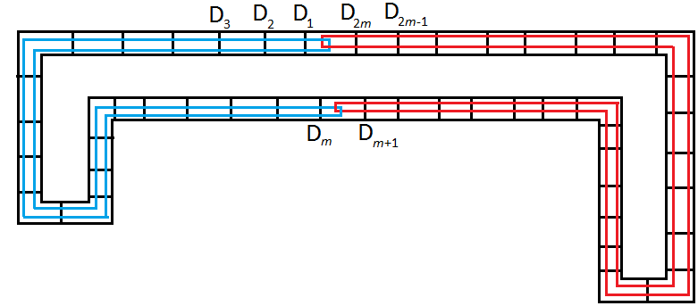
Figure 2. The tubes $\tau_{11}$ (blue) and $\tau_{12}$ (red) inside $\tau_{1}$.

Due to the equivalence of initial packages, there exists a diffeomorphism $h_{1}\colon t\to t$ which is the identity in a neighborhood of $t\setminus(\tau_{1}\cup\tau_{2})$ and satisfies $h_{1}(\phi_{1j}(t))=\phi^{\prime}_{1j}(\tau_{1})$ for $j=1,2$. Similar rearrangement is possible in the solid torus $\tau_{2}$.

If $m=1$, then $h_{1}$ satisfies the condition $\operatorname{diam}{h_{1}(\phi_{w}(t))}<\varepsilon$ for all words $w$ of length $k=2$.

Step 2. Suppose that $m\geq 2$. We focus on the solid torus $\tau_{11}=\phi^{\prime}_{11}(\tau_{1})$; constructions in other tori $\tau_{ij}=\phi^{\prime}_{ij}(\tau_{i})$ are verbatim. Following the idea in Step 1, we fix smooth curves $\sigma_{111}$ and $\sigma_{112}$ in $\tau_{11}$ as in Figure 3 linked between the disks $D_{1}$ and $D_{2}$ and the other between $D_{m-1}$ and $D_{m}$. We also require that $\sigma_{111}$ intersects exactly $D_{1},\dots,D_{m-1}$ and $\sigma_{112}$ intersects exactly $D_{2},\dots,D_{m}$. Furthermore, if $m\geq 3$, for each $i=1,2$, we require that $\sigma_{11i}$ intersects each of $D_{2},\dots,D_{m-1}$ exactly at $2$ points.

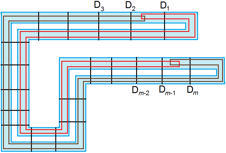
Figure 3. The tubes $\tau_{111}$ (brown) and $\tau_{112}$ (red) inside $\tau_{11}$.

As in Step 1, we fix $\delta_{2}\in(0,\delta_{1})$ and an initial package $\mathfrak{I}^{\prime}_{3}=(\tau_{11};\phi^{\prime}_{111},\phi^{\prime}_{112})$ so that $\phi^{\prime}_{11i}(\tau_{11})=B^{3}(\sigma_{11i},\delta_{2})$ for $i=1,2$. Similarly with $\sigma_{111},\sigma_{112}$, we may assume that $\tau_{111}=\phi^{\prime}_{111}(\tau_{11})$ intersects exactly $D_{1},\dots,D_{m-1}$ and $\tau_{112}=\phi^{\prime}_{112}(\tau_{11})$ intersects exactly $D_{2},\dots,D_{m}$.

There exists now a diffeomorphism $h_{2}\colon t\to t$ which coincides with $h_{1}$ on $t\setminus\bigcup_{|w|=2}\tau_{w}$. Moreover, if $m=2$, $\operatorname{diam}{h(\phi_{w}(t))}<\varepsilon$ for $|w|=3$.

Induction assumption. Suppose we have continued the process for $k\geq 1$ steps and that there exists $\delta_{k}>0$ so that, for each $w\in\mathcal{W}_{2}$ of length $k+1$,

• the solid torus $\tau_{w}$ is the $\delta_{k}$-neighborhood of the smooth core curve $\sigma_{w}$ of $\tau_{w}$,

• $\sigma_{w}$ intersects exactly $m-k+1$ consecutive disks in $\{D_{1},\ldots,D_{2m}\}$,

• $\sigma_{w}$ intersects $m-k$ consecutive disks in $\{D_{1},\ldots,D_{2m}\}$ at exactly two points.

Step $k+1$. Let $w$ be a word of length $k+1$ and let $j\in\mathbb{N}$ be such that $\sigma_{w}$ intersects disks $D_{j},\dots,D_{j+m-k}$. By the previous step, we may assume that $\sigma_{w}$ intersects disks $D_{j+1},\ldots,D_{j+m-k}$ at exactly two points.

Let $\sigma_{w1}$ and $\sigma_{w2}$ be smooth pair-wise disjoint curves in $\tau_{w}$ with the following properties:

• $\sigma_{w1}$ and $\sigma_{w2}$ link as in Figure 1, that is, $(\tau_{w},\sigma_{w1}\cup\sigma_{w2})$ and $(\tau_{0},\sigma_{1}\cup\sigma_{2})$ are diffeomorphic as pairs;

• $\sigma_{w1}$ and $\sigma_{w2}$ link between $D_{j}$ and $D_{j+1}$ and between $D_{j+m-k-1}$ and $D_{j+m-k}$;

• there exists $j\in\{1,\ldots,2m\}$ so that $\sigma_{w1}$ intersects exactly disks $D_{j},\dots,D_{j+m-k-1}$ and $\sigma_{w2}$ exactly disks $D_{j+1},\dots,D_{j+m-k}$; and

• if $m\geq k+2$, $\sigma_{wi}$ intersects each disk $D_{j+1},\dots D_{j+m-k-1}$ exactly at $2$ points for $i=1,2$.

Let now $\delta_{k+1}\in(0,\delta_{k})$ be such that there exists smooth embeddings $\phi^{\prime}_{wi}\colon\tau_{w}\to\tau_{w}$ for which $\phi^{\prime}_{wi}(\tau_{w})=B^{3}(\sigma_{wi},\delta_{k+1})$ and $(\tau_{w};\phi^{\prime}_{w1},\phi^{\prime}_{w2})$ is equivalent to the initial package $\mathfrak{I}_{B}$.

We conclude again that there exists a diffeomorphism $h_{k+1}\colon t\to t$ which agrees with $h_{k}$ in $t\setminus\bigcup_{|v|=k+1}\tau_{v}$ and satisfies $h_{k+1}(\phi_{wi}(t))=\phi^{\prime}_{wi}(\tau_{w})$ for each $|w|=k$ and $i=1,2$. This concludes the induction step.

Step $m$; end of the process. Suppose that we have reached the step $k=m$. Then, for each $w\in\mathcal{W}_{2}$ of length $m+1$, the solid torus $\tau_{w}$ intersects exactly one of the disks $D_{1},\ldots,D_{2m}$. Thus $\operatorname{diam}{h_{m}(t_{w})}<\varepsilon$ for $|w|=m+1$. This completes the proof.

3.3.2. Proof of Lemma 3.4

We apply Bing’s idea to rearrange the Blankinship rings $\mathbb{T}_{w}$ (or equivalently rings $\vartheta(\mathbb{T}_{w})$) so that the diameters decrease to zero as $|w|\to\infty$. We discuss the details of the proof of Lemma 3.4 only in dimension $n=4$ for brevity. The homeomorphism $\hat{\varrho}$ is obtained similarly in higher dimensions.

We use notation and constructions from the proof of Lemma 3.3. In the forthcoming steps, we endow each curve $\sigma\subset\mathbb{R}^{3}$ with the restriction of the Euclidean metric and denote this metric by $d_{\sigma}$. We also consider product spaces $(\sigma,d_{\sigma})\times\mathbb{B}^{2}(\delta)$ and $(\sigma,d_{\sigma})\times\mathbb{B}^{2}(\delta)\times(\hat{\sigma},d_{\hat{\sigma}})$ for $\delta>0$, which we endow with the $\ell^{2}$-metrics

$$d_{\sigma,\delta}((x,z),(x^{\prime},z^{\prime}))=\left(d_{\sigma}(x,x^{\prime})^{2}+|z-z^{\prime}|^{2}\right)^{1/2}$$

and

$$d_{\sigma,\delta,\hat{\sigma}}((x,z,y),(x^{\prime},z^{\prime},y^{\prime}))=\left(d_{\sigma}(x,x^{\prime})^{2}+|z-z^{\prime}|^{2}+d_{\hat{\sigma}}(y,y^{\prime})^{2}\right)^{1/2},$$

respectively, where $(x,z),(x^{\prime},z^{\prime})\in(\sigma,d_{\sigma})\times\mathbb{B}^{2}(\delta)$ and $(x,z,y),(x^{\prime},z^{\prime},y^{\prime})\in(\sigma,d_{\sigma})\times\mathbb{B}^{2}(\delta)\times(\hat{\sigma},d_{\hat{\sigma}})$.

We begin with a simple observation on bilipschitz parametrizations of tubular neighborhoods of smooth curves in $\mathbb{R}^{3}$, which we record as a lemma; see [19, Theorem 9.20]. Recall that

$$B^{3}(\sigma,\delta)=\{x\in\mathbb{R}^{3}\colon\text{dist}(x,\sigma)\leq\delta\}$$

denotes a $\delta$-neighborhood of $\sigma$ in $\mathbb{R}^{3}$.

Lemma 3.5.

Suppose $\sigma\subset\mathbb{R}^{n}$ is a closed smooth simple curve. Then, for each $L>1$, there exists $\delta>0$ and an $L$-bilipschitz diffeomorphism

$$e_{\sigma,\delta}\colon(\sigma,d_{\sigma})\times\mathbb{B}^{2}(\delta)\to B^{3}(\sigma,\delta)$$

such that $e_{\sigma,\delta}(x,0)=x$ for all $x\in\sigma$.

Let $\sigma\subset\mathbb{R}^{3}$ be a smooth simple closed curve and $\delta>0$. Given a diffeomorphism $e_{\sigma,\delta}$ as in Lemma 3.5, we define a diffeomorphism $\hat{e}_{\sigma,\delta}\colon\mathbb{B}^{2}(\delta)\times(\sigma,d_{\sigma})\to B^{3}(\sigma,\delta)$ by $\hat{e}_{\sigma,\delta}(u,x)=e_{\sigma,\delta}(x,u)$. If $\hat{\sigma}$ is another smooth simple closed curve in $\mathbb{R}^{3}$, we call a diffeomorphism

$$G_{\sigma,\delta,\hat{\sigma}}\colon B^{3}(\sigma,\delta)\times(\hat{\sigma},d_{\hat{\sigma}})\to(\sigma,d_{\sigma})\times B^{3}(\hat{\sigma},\delta)$$

defined by

$$G_{\sigma,\delta,\hat{\sigma}}=(\mathrm{id}_{\sigma}\times\hat{e}_{\hat{\sigma},\delta})\circ(e_{\sigma,\delta}\times\mathrm{id}_{\hat{\sigma}})^{-1}$$

a neighborhood switch.

To simplify the notation in the proof of Lemma 3.4, we define, for each word $w=i_{1}\cdots i_{k}$ and $\hat{w}=j_{1}\cdots j_{\ell}$ in $\mathcal{W}_{2}$, their interlace $[w,\hat{w}]\in\mathcal{W}_{2}$ by

$$[w,\hat{w}]=\left\{\begin{array}[]{ll}i_{1}j_{1}i_{2}j_{2}\cdots i_{k}j_{k}j_{k+1}\cdots j_{\ell},&\mathrm{if}\ \ell\geq k,\\ i_{1}j_{1}i_{2}j_{2}\cdots i_{\ell}j_{\ell}i_{\ell+1}\cdots i_{k},&\mathrm{if}\ell<k.\end{array}\right.$$

Proof of Lemma 3.4.

Let $\varepsilon>0$. Since the diffeomorphism $\phi_{w}\colon t\to t_{w}$ is absolutely continuous for each $w\in\mathcal{W}_{2}$, it suffices to consider only the case $k=0$. In what follows, we denote $\mathbb{T}=\mathbb{S}^{1}\times\mathbb{B}^{2}\times\mathbb{S}^{1}$ and $\mathbb{T}_{w}=\tilde{\varphi}_{w}(\mathbb{T})$ for $w\in\mathcal{W}_{2}$. For completion, we set $\sigma_{0}=\hat{\sigma}_{0}=\mathbb{S}^{1}\subset\mathbb{R}^{3}$.

We construct iteratively a finite ordered tree $(T_{u})_{|u|\leq m}$ equivalent to $\mathfrak{I}_{B,n}$, where $u\in\mathcal{W}_{2}$ has length at most $2m$ and $\operatorname{diam}T_{u}<\varepsilon$ for each $|u|=2m$. The required $4$-tubes $T_{u}$ and the level $m$ are found by showing that there exists $\delta_{0}>0$ so that, if $m\in\mathbb{N}$ is the level associated to diameter $\varepsilon^{\prime}=\varepsilon\delta_{0}/20$ in Lemma 3.3, we find $4$-tubes $T_{u}$ for which there exists $(\delta_{0}/8)$-bilipschitz diffeomorphisms $T_{[w,\hat{w}]}\to(\sigma_{w},d_{\sigma_{w}})\times\mathbb{B}^{2}(\delta_{m})\times(\sigma_{\hat{w}},d_{\sigma_{\hat{w}}})$ for each $w,\hat{w}\in\mathcal{W}_{2}$ of length $m$, where $\sigma_{w}$ and $\sigma_{\hat{w}}$ are core curves of $3$-tubes $\tau_{w}$ and $\tau_{\hat{w}}$, respectively, as in the proof of Lemma 3.3. The diameter bound follows then from diameter bounds of curves $\sigma_{w}$.

Roughly speaking, the curves $\sigma_{w}$ and $\sigma_{\hat{w}}$ are obtained by applying Bing’s shrinking rearrangement in the two $\mathbb{S}^{1}$ directions of $\mathbb{T}$. In Steps $(k,1)$ below, $k\in\mathbb{N}\cup\{0\}$, we apply the shrinking rearrangement for the first direction and Steps $(k,2)$ for the second.

Fix $\delta_{0}\in(0,1)$ small enough so that the diffeomorphism $e_{\sigma_{0},\delta_{0}}$ of Lemma 3.5 is $2$-bilipschitz. Set $\tau_{0}=B^{3}(\sigma_{0},\delta_{0})$ and define $R_{0}\colon\mathbb{T}\to\tau_{0}\times\hat{\sigma}_{0}$ by

$$(x,u,y)\mapsto(e_{\sigma_{0},\delta_{0}}(x,\delta_{0}u),y).$$

Then $R_{0}$ is a $(2/\delta_{0})$-bilipschitz diffeomorphism.

Step (0,1). Let $\tau_{1}=B^{3}(\sigma_{1},\delta_{1})$ and $\tau_{2}=B^{3}(\sigma_{2},\delta_{1})$ be $3$-tubes in $\tau_{0}$, where $\sigma_{1}$ and $\sigma_{2}$ are smooth simple curves linked in $\tau_{0}$ as in Figure 1, and $\delta_{1}<\varepsilon\delta_{0}/20$. We choose $\delta_{1}$ small enough so that the diffeomorphisms $e_{\sigma_{1},\delta_{1}}$ and $e_{\sigma_{2},\delta_{1}}$, in Lemma 3.5, and the diffeomorphism $\hat{e}_{\hat{\sigma}_{0},\delta_{1}}$, associated to $e_{\hat{\sigma},\delta_{1}}$, are $2^{1/2}$-bilipschitz. For each $i=1,2$, let $\phi_{i}\colon\tau_{0}\to\tau_{0}$ be a diffeomorphism with $\phi_{i}(\tau_{0})=\tau_{i}$. Define $\Phi_{i}\colon\mathbb{T}\to\mathbb{T}$ by $\Phi_{i}=R_{0}^{-1}\circ(\phi_{i}\times\mathrm{id})\circ R_{0}$ and set $T_{i}=\Phi_{i}(\mathbb{T})\subset\mathbb{T}$. Note that the initial package $(\mathbb{T};\Phi_{1},\Phi_{2})$ is conjugate to $(\mathbb{T};\tilde{\varphi}_{1},\tilde{\varphi}_{2})$ and that the diagram

commutes.

Step (0,2). Set $\hat{\tau}_{0}=B^{3}(\hat{\sigma}_{0},\delta_{1})$ and, for $i=1,2$, let $R_{i}\colon T_{i}\to(\sigma_{i},d_{\sigma_{i}})\times\hat{\tau}_{0}$ be the mapping

$$R_{i}=G_{\sigma_{i},\delta_{1},\hat{\sigma}_{0}}\circ R_{0}.$$

Let $\hat{\tau}_{1}=B^{3}(\hat{\sigma}_{1},\hat{\delta}_{1})$ and $\hat{\tau}_{2}=B^{3}(\hat{\sigma}_{2},\hat{\delta}_{1})$ be $3$-tubes in $\hat{\tau}_{0}$, where $\hat{\sigma}_{1}$ and $\hat{\sigma}_{2}$ are smooth simple curves, linked inside $\hat{\tau}_{0}$ as in Figure 1, and $\hat{\delta}_{1}<\delta_{1}$. Moreover, we may assume that $\hat{\delta}_{1}$ is small enough so that the diffeomorphisms $\hat{e}_{\hat{\sigma}_{j},\hat{\delta}_{1}}$ and $e_{\sigma_{i},\hat{\delta}_{1}}$ are $2^{1/4}$-bilipschitz for $i,j\in\{1,2\}$. For each $j=1,2$, let $\hat{\phi}_{j}\colon\hat{\tau}_{0}\to\hat{\tau}_{0}$ be a diffeomorphism satisfying $\hat{\phi}_{j}(\tau_{0})=\hat{\tau}_{j}$. Define also $\Phi_{ij}\colon T_{i}\to T_{i}$ by $\Phi_{ij}=R_{i}^{-1}\circ(\mathrm{id}\times\phi_{j})\circ R_{i}$ and set $T_{ij}=\Phi_{ij}(T_{i})\subset T_{i}$. Then the initial package $(T_{i};\Phi_{i1},\Phi_{i2})$ is conjugate to $(\mathbb{T};\tilde{\varphi}_{1},\tilde{\varphi}_{2})$ and the diagram

commutes.

Let $m\in\mathbb{N}$ be the number of steps needed in Bing’s shrinking procedure for $\tau_{0}$ and $\varepsilon\delta_{0}/20$. We may assume that the same number of $m$ steps is needed in Bing’s shrinking procedure for the simple curve $\hat{\tau}_{0}$ and diameter $\varepsilon\delta_{0}/20$. We now apply Steps $1$ to $m$ of Bing’s shrinking procedure to both curves $\tau_{0}$ and $\hat{\tau}_{0}$.

Suppose that after Step $(k,1)$ and Step $(k,2)$ we have obtained radii

$$\delta_{0}>\hat{\delta}_{0}>\cdots>\delta_{k}>\hat{\delta}_{k}>0$$

and, for each $\ell\in\{1,\ldots,k\}$, $w=i_{1}\cdots i_{\ell}$ and $\hat{w}=j_{1}\cdots j_{\ell-1}$ in $\mathcal{W}_{2}$, and $j=1,2$, we have

1. smooth closed simple curves $\sigma_{w}$ and $\hat{\sigma}_{\hat{w}j}$ as in the Step $\ell$ of Bing’s shrinking procedure so that $\tau_{w}=B^{3}(\sigma_{w},\delta_{\ell})$ and $\hat{\tau}_{\hat{w}j}=B^{3}(\hat{\sigma}_{\hat{w}j},\hat{\delta}_{\ell})$ are $3$-tubes;

2. a $4$-tube $T_{[w,\hat{w}j]}$ and a diffeomorphic embedding

   $$\Phi_{[w,\hat{w}j]}\colon T_{[w,\hat{w}]}\to T_{[w,\hat{w}]}$$

   for which $T_{[w,\hat{w}j]}=\Phi_{[w,\hat{w}j]}(T_{[w,\hat{w}]})$ and $(T_{[w,\hat{w}]};\Phi_{[w,\hat{w}1]},\Phi_{[w,\hat{w}2]})$ is conjugate to $(\mathbb{T};\tilde{\varphi}_{1},\tilde{\varphi}_{2})$;

3. diffeomorphisms $e_{\sigma_{w},\hat{\delta}_{k}}$ and $\hat{e}_{\hat{\sigma}_{\hat{w}j,\hat{\delta}_{k}}}$ as in Lemma 3.5 which are $2^{2^{-2k}}$-bilipschitz; and

4. a diffeomorphism $R_{[w,\hat{w}]}\colon T_{[w,\hat{w}j]}\to(\sigma_{w},d_{\sigma_{w}})\times\hat{\tau}_{\hat{w}}$ satisfying

   $$R_{[w,\hat{w}]}=G_{\sigma_{w},\delta_{k},\hat{\sigma}_{\hat{w}}}\circ R_{[w,\hat{w}j]}.$$

Step $(k+1,1)$. Let $w,\hat{w}\in\mathcal{W}_{2}$ be words of length $|w|=k$ and $|\hat{w}|=k-1$. We define

$$R_{[w,\hat{w}j]}\colon T_{[w,\hat{w}j]}\to\tau_{w}\times(\hat{\sigma}_{\hat{w}j},d_{\hat{\sigma}_{\hat{w}j}})$$

for $j=1,2$ by

$$R_{[w,\hat{w}j]}=(G_{\sigma_{w},\hat{\delta}_{k},\hat{\sigma}_{\hat{w}j}})^{-1}\circ R_{[w,\hat{w}]}.$$

Let $\sigma_{w1}$ and $\sigma_{w2}$ be smooth simple closed curves in $\tau_{w}$ as in Step $k+1$ of Bing’s shrinking procedure, and $\delta_{k+1}<\hat{\delta}_{k}$ be small enough so that the diffeomorphisms $e_{\sigma_{wi},\delta_{k+1}}$ and $\hat{e}_{\hat{\sigma}_{\hat{w}j},\delta_{k+1}}$ of Lemma 3.5 are $2^{2^{-2k-1}}$-bilipschitz for $i,j\in\{1,2\}$.

For $i=1,2$, let $\tau_{wi}=B^{3}(\sigma_{wi},\delta_{k+1})$ and $\phi_{wi}\colon\tau_{w}\to\tau_{wi}$ be a diffeomorphism. Define also, for $j=1,2$,

$$\Phi_{[wi,\hat{w}j]}\colon T_{[w,\hat{w}j]}\to T_{[w,\hat{w}j]}$$

by

$$\Phi_{[wi,\hat{w}j]}=R_{[w,\hat{w}j]}^{-1}\circ(\phi_{wi}\times\mathrm{id})\circ R_{[w,\hat{w}j]},$$

and set

$$T_{[wi,\hat{w}j]}=\Phi_{[wi,\hat{w}j]}(T_{[w,\hat{w}j]})\subset T_{[w,\hat{w}j]}.$$

Step $(k+1,2)$. For $w$ and $\hat{w}$ in $\mathcal{W}_{2}$ of length $k$, define

$$R_{[wi,\hat{w}]}\colon T_{[wi,\hat{w}]}\to(\sigma_{wi},d_{\sigma_{wi}})\times\hat{\tau}_{\hat{w}}$$

for $i=1,2$, by

$$R_{[wi,\hat{w}]}=G_{\sigma_{wi},\delta_{k+1},\hat{\sigma}_{\hat{w}}}\circ R_{[w,\hat{w}]}.$$

Let $\sigma_{\hat{w}1}$ and $\sigma_{\hat{w}2}$ be two smooth simple closed curves in $\hat{\tau}_{\hat{w}}$ as in Step $k+1$ of Bing’s shrinking procedure, and $\hat{\delta}_{k+1}<\delta_{k+1}$ be small enough so that the diffeomorphisms $e_{\sigma_{wi},\hat{\delta}_{k+1}}$ and $e_{\hat{\sigma}_{\hat{w}j},\hat{\delta}_{k+1}}$ of Lemma 3.5 are $2^{2^{-2k-2}}$-bilipschitz for $i=1,2$.

For each $j\in\{1,2\}$, let $\hat{\tau}_{\hat{w}j}=B^{3}(\hat{\sigma}_{\hat{w}j},\hat{\delta}_{k+1})$ and $\hat{\phi}_{\hat{w}j}\colon\hat{\tau}_{\hat{w}}\to\hat{\tau}_{\hat{w}j}$ be a diffeomorphism. Define now

$$\Phi_{[wi,\hat{w}j]}\colon T_{[wi,\hat{w}]}\to T_{[wi,\hat{w}]}$$

for $i,j\in\{1,2\}$ by

$$\Phi_{[wi,\hat{w}j]}=R_{[wi,\hat{w}]}^{-1}\circ(\mathrm{id}\times\hat{\phi}_{wi})\circ R_{[wi,\hat{w}j]}$$

and set

$$T_{[wi,\hat{w}j]}=\Phi_{[wi,\hat{w}j]}(T_{[wi,\hat{w}]})\subset T_{[wi,\hat{w}]}$$

for each $i$ and $j$.

Suppose we have completed Step $(m,2)$ and let $w=i_{1}\cdots i_{m}$ and $\hat{w}=j_{1}\cdots j_{m}$ be words in $\mathcal{W}_{2}$. By the choice of radii $\delta_{\ell}$ and $\hat{\delta}_{\ell}$ for $\ell=1,\ldots,m$, the diffeomorphism

$$R_{[w,j_{1}\cdots j_{m-1}]}\colon T_{[w,\hat{w}]}\to B^{3}(\sigma_{w},\delta_{m})\times(\hat{\sigma}_{\hat{w}},d_{\hat{\sigma}_{\hat{w}}}),$$

is $(8/\delta_{0})$-bilipschitz. Indeed, denote, for each $\ell\in\{1,\ldots,m\}$,$w_{\ell}=i_{1}\cdots i_{\ell}$ and $\hat{w}_{\ell}=j_{1}\cdots j_{\ell}$. Then

$$R_{[w,\hat{w}_{m-1}]} = G_{\sigma_{w},\delta_{m},\hat{\sigma}_{\hat{w}_{m-1}}}\circ R_{[w_{m-1},\hat{w}_{m-1}]}$$

$$= G_{\sigma_{w},\delta_{m},\hat{\sigma}_{\hat{w}_{m-1}}}\circ(G_{\sigma_{w_{m-1}},\hat{\delta}_{m-1},\hat{\sigma}_{\hat{w}_{m-1}}})^{-1}\circ R_{[w_{m-1},\hat{w}_{m-2}]}$$

$$= G^{\prime}_{m}\circ\cdots\circ G^{\prime}_{2}\circ G_{\sigma_{i_{1}},\delta_{1},\hat{\sigma}_{0}}\circ R_{0},$$

where

$$G^{\prime}_{\ell}=G_{\sigma_{w_{\ell}},\delta_{\ell},\hat{\sigma}_{\hat{w}_{\ell-1}}}\circ(G_{\sigma_{w_{\ell-1}},\hat{\delta}_{\ell-1},\hat{\sigma}_{\hat{w}_{\ell-1}}})^{-1}$$

for each $\ell=2,\ldots,m$.

Since $\operatorname{diam}{\sigma_{w}}<\varepsilon\delta_{0}/20$ and $\operatorname{diam}{\hat{\sigma}_{\hat{w}}}<\varepsilon\delta_{0}/20$,

$$\operatorname{diam}{T_{[w,\hat{w}]}}\leq 8(\delta_{0})^{-1}(\operatorname{diam}{\sigma_{w}}+\operatorname{diam}{\hat{\sigma}_{\hat{w}}}+\delta_{m})<\varepsilon.$$

This concludes the proof of Lemma 3.4. ∎

Proof of Proposition 3.2.

The proof of Proposition 3.2 is identical to the discussion in [3, Section 3.III]. By Lemma 3.4, there exists $k_{1}\in\mathbb{N}$ and a diffeomorphism $\hat{\varrho}_{1}\colon\mathbb{S}^{n}\to\mathbb{S}^{n}$ which leaves each point of $\mathbb{S}^{n}\setminus(T_{1}\cup T_{2})$ fixed and maps each torus $T_{w}$, for $|w|=k_{1}$, into a set of diameter less than $1$. Then, by uniform continuity of $(\hat{\varrho}_{1})^{-1}$, there exists $\varepsilon>0$ for which a set $E\subset\mathbb{S}^{n}$ has diameter less than $1/2$ if $\operatorname{diam}{\hat{\varrho}_{1}(E)}<\varepsilon$. Reapplying Lemma 3.4, we find an integer $k_{2}>k_{1}$ and a diffeomorphism $\hat{\varrho}_{2}^{\prime}\colon\mathbb{S}^{n}\to\mathbb{S}^{n}$ which leaves each point of $\mathbb{S}^{n}\setminus{\bigcup_{|w|=k_{1}}T_{w}}$ fixed and maps each torus $T_{w}$, for $|w|=k_{2}$, into a set of diameter less than $\varepsilon$. Then $\hat{\varrho}_{2}=\hat{\varrho}_{1}\circ\hat{\varrho}_{2}^{\prime}$ is a diffeomorphism of $\mathbb{S}^{n}$ into itself which maps each torus $T_{w}$, for $|w|=k_{1}$, to a set of diameter $1$ and each torus $T_{w}$, for $|w|=k_{2}$, to a set of diameter $1/2$.

Iterating this procedure, we find a sequence of diffeomorphisms $\hat{\varrho}_{1},\hat{\varrho}_{2},\dots$ and integers $k_{1}<k_{2}<\cdots$ for which $\hat{\varrho}_{m+1}|\mathbb{S}^{n}\setminus\bigcup_{|w|=k_{m}}\mathbb{T}_{w}=\hat{\varrho}_{m}|\mathbb{S}^{n}\setminus\bigcup_{|w|=k_{m}}\mathbb{T}_{w}$, and $\operatorname{diam}{\hat{\varrho}_{m}(\mathbb{T}_{w})}<1/m$ for each $|w|=k_{m}$. The limit $\hat{\rho}=\lim_{m\to\infty}\hat{\varrho}_{m}$ is a map $\hat{\rho}\colon\mathbb{S}^{n}\to\mathbb{S}^{n}$ for which $\hat{\rho}(\mathcal{S}(\mathfrak{I}_{B,n}))$ is a Cantor set and the restriction $\hat{\rho}|S^{n}\setminus\mathcal{S}(\mathfrak{I}_{B,n})\colon\mathbb{S}^{n}\setminus\mathcal{S}(\mathfrak{I}_{B,n})\to\hat{\rho}(\mathbb{S}^{n})\setminus\hat{\rho}(\mathcal{S}(\mathfrak{I}_{B,n})$ is a diffeomorphism. The proof is complete. ∎

3.4. An almost smooth metric on $\mathbb{S}^{n}$ associated to $\mathbb{S}^{n}/\mathrm{BB}$

As a direct corollary of Propositions 3.1 and 3.2, we obtain an almost smooth metric on $\mathbb{S}^{n}$ having the Bing–Blankinship Cantor set as a singular set.

Corollary 3.6.

Let $n\geq 3$, $\mathfrak{I}_{B,n}$ be a Bing–Blankinship initial package, and let $\hat{\rho}\colon\mathbb{S}^{n}\to\mathbb{S}^{n}$ be a map as in Proposition 3.2. Let also $E=\hat{\rho}(\mathcal{S}(\mathfrak{I}_{B,n}))$.

Then, there exists a Cantor set $E\subset\mathbb{S}^{n}$ and a Riemannian metric $g$ in $\mathbb{S}^{n}\setminus E$ for which the completion of the associated length metric $d$ is Ahlfors $n$-regular and linearly locally contractible.

Proof.

Let $\lambda\in(0,2^{-1/n})$ and let $\tilde{\rho}\colon\mathbb{S}^{n}\to\mathbb{S}^{n+1}$ be the mapping in Proposition 3.1. We set $g$ to be the Riemannian metric $(\tilde{\rho}\circ\hat{\rho}^{-1}|\mathbb{S}^{n}\setminus E)^{*}g_{0}$, where $g_{0}$ is the Riemannian metric on $\mathbb{S}^{n+1}$. Let $d$ be the completion of the length metric associated to $g$.

Let $\rho^{\prime}\colon\mathbb{S}^{n}/\mathrm{BB}\to\mathbb{S}^{n}$ be the homeomorphism in Proposition 3.2 and $d^{\prime}$ the pull-back metric $d^{\prime}(x,y)=d((\rho^{\prime}\circ\vartheta^{\prime})(x),(\rho^{\prime}\circ\vartheta^{\prime})(y))$ on $\mathbb{T}/G_{\mathfrak{I}_{B,n}}$. Then $d^{\prime}$ is a Semmes metric on $\mathbb{S}^{n}/\mathrm{BB}$, with respect to the initial package $\mathfrak{I}_{B,n}$, of scaling constant $\lambda$. Thus $(\mathbb{T}/G_{\mathfrak{I}_{B,n}},d^{\prime})$ is Ahlfors $n$-regular and LLC by Lemmas 2.2 and 2.3. Thus also $(\mathbb{S}^{n},d)$ is Ahlfors $n$-regular and LLC; see e.g. [14, Proposition 7.8] and [14, Proposition 7.9] for details. ∎

4. Virtually interior-essential maps

In this section we prove a Freedman-Skora type result that, for a virtually interior essential map $\Phi\colon(\mathbb{B}^{2},\partial\mathbb{B}^{2})\to(\mathbb{T},\partial\mathbb{T})$, the number of essential intersections $\Phi(\mathbb{B}^{2})\cap\bigcup_{|w|=k}\tilde{\varphi}_{w}(\mathbb{T})$ is at least $2^{k}$. We begin by introducing terminology.

Let $\omega\subset\mathbb{B}^{2}$ be a compact and connected $2$-manifold with boundary. The smallest $2$-cell $D_{\omega}$ in $\mathbb{B}^{2}$ containing $\omega$ is the hull of $\omega$ in $\mathbb{B}^{2}$, that is, $D_{\omega}$ is the unique $2$-cell in $\mathbb{B}^{2}$ containing $\omega$ for which $\partial D_{\omega}$ is a component of $\partial\omega$. We call $\partial D_{\omega}$ the outer boundary of $\omega$ and $\partial\omega\setminus\partial D_{\omega}$ the inner boundary of $\omega$.

Let $M$ be an $n$-manifold with boundary. A map of pairs $\Phi\colon(\omega,\partial\omega)\to(M,\partial M)$ is interior-inessential if there exists a map $\Phi^{\prime}\colon\omega\to\partial M$ for which $\Phi^{\prime}|\partial\omega=\Phi|\partial\omega$. Otherwise, $\Phi$ is interior-essential. Further, a map of pairs $\Phi\colon(\omega,\partial\omega)\to(M,\partial M)$ is virtually interior-essential if there exists an interior-essential extension $\hat{\Phi}\colon(D_{\omega},\partial D_{\omega})\to(M,\partial M)$ of $\Phi$ satisfying $\hat{\Phi}(D\setminus\omega)\subset\partial M$.

Let $N\subset\mathrm{int}M$ be an $n$-manifold with boundary and $\omega\subset\mathbb{B}^{2}$ a compact and connected $2$-manifold with boundary. A map $\Phi\colon(\omega,\partial\omega)\to(M,\partial M)$ intersects $N$ transversely if $\Phi^{-1}(\partial N)$ is a closed $1$-manifold, i.e. $\Phi^{-1}(\partial N)$ is a finite pair-wise disjoint collection of circles in $\omega$. In particular, components of $\Phi^{-1}(N)$ are compact and connected $2$-manifolds with boundary if $\Phi$ intersects $N$ transversely. Note that each map $(\omega,\partial\omega)\to(M,\partial M)$ is homotopic, relative to the boundary $\partial\omega$, to a map which intersects $N$ transversely.

For a mapping $\Phi\colon\omega\to M$ intersecting $N$ transversely, we denote by $\Omega(\Phi;N)$ the set of all components $\omega^{\prime}\subset\Phi^{-1}(N)$ for which $\Phi|\omega^{\prime}\colon(\omega^{\prime},\partial\omega^{\prime})\to(N,\partial N)$ is interior essential. A component $\omega^{\prime}\in\Omega(\Phi;N)$ is innermost if $D_{\omega^{\prime}}\setminus\omega^{\prime}$ has no element in $\Omega(\Phi;N)$. We emphasize that $\Omega(\Phi;N)$ is a finite set, since $\Phi^{-1}(\partial N)$ has finitely many components.

The main result of this section is the following proposition. Note that, although not explicitly mentioned, we consider a fixed initial package $\mathfrak{I}_{B,n}=(\mathbb{T};\tilde{\varphi}_{1},\tilde{\varphi}_{2})$ for the Bing-Blankinship decomposition.

Proposition 4.1.

Let $\omega\subset\mathbb{B}^{2}$ be a compact and connected $2$-manifold, and suppose $\Phi\colon(\omega,\partial\omega)\to(\mathbb{T},\partial\mathbb{T})$ is a virtually interior-essential map meeting $\mathbb{T}_{1}\cup\mathbb{T}_{2}$ transversely. Then there exists at least two virtually interior essential components in $\Omega(\Phi;\mathbb{T}_{1}\cup\mathbb{T}_{2})$.

Since $(\mathbb{T}_{w},\mathbb{T}_{w1}\cup\mathbb{T}_{w2})$ is homeomorphic, as pairs, to $(\mathbb{T},\mathbb{T}_{1}\cup\mathbb{T}_{2})$, a simple induction argument yields the following corollary.

Corollary 4.2.

Let $\Phi\colon(\mathbb{B}^{2},\partial\mathbb{B}^{2})\to(\mathbb{T},\partial\mathbb{T})$ be an interior essential map which meets each $\mathbb{T}_{w}$, for $w\in\mathcal{W}_{2}$, transversely. Then

$$\#\Omega(\Phi;\bigcup_{|w|=k}\mathbb{T}_{w})\geq 2^{k}$$

for each $k\geq 0$.

The proof of Proposition 4.1 is based on a homological argument as in Freedman and Skora [9, Lemma 2.5]. Before the proof we make first some well-known preliminary observations.

Lemma 4.3.

The homomorphism $\pi_{1}(\partial\mathbb{T})\to\pi_{1}(\mathbb{T}\setminus(\mathbb{T}_{1}\cup\mathbb{T}_{2}))$, induced by the inclusion $\partial\mathbb{T}\to\mathbb{T}\setminus(\mathbb{T}_{1}\cup\mathbb{T}_{2})$, is a monomorphism. Furthermore, the homomorphism $\pi_{1}(\partial\mathbb{T}_{i})\to\pi_{1}(\mathbb{T}\setminus\mathrm{int}(\mathbb{T}_{1}\cup\mathbb{T}_{2}))$, induced by the inclusion $\partial\mathbb{T}_{i}\to\mathbb{T}\setminus\mathrm{int}(\mathbb{T}_{1}\cup\mathbb{T}_{2})$, is a monomorphism for $i=1,2$.

Proof.

For $n=3$, i.e. for the Bing double, see [7, Lemmas 2.4 and 2.5]. For $n\geq 3$, it suffices to observe that

$$\mathbb{T}=(\mathbb{B}^{2}\times\mathbb{S}^{1})\times(\mathbb{S}^{1})^{n-3}$$

and

$$\mathbb{T}_{i}=\varphi_{i}(\mathbb{B}^{2}\times\mathbb{S}^{1})\times(\mathbb{S}^{1})^{n-3},$$

where $\varphi_{i}\colon\mathbb{B}^{2}\times\mathbb{S}^{1}\to\mathbb{B}^{2}\times\mathbb{S}^{1}$, for $i=1,2$, is the embedding in the initial package of the Bing double. ∎

Corollary 4.4.

Let $\Phi\colon(\mathbb{B}^{2},\partial\mathbb{B}^{2})\to(\mathbb{T},\partial\mathbb{T})$ be an interior essential map. Then $\Phi^{-1}(\mathbb{T}_{1}\cap\mathbb{T}_{2})\neq\emptyset$. Furthermore, $\Omega(\Phi;\mathbb{T}_{1}\cup\mathbb{T}_{2})\neq\emptyset$ if $\Phi$ meets $\mathbb{T}_{1}\cup\mathbb{T}_{2}$ transversely.

Proof.

Suppose $\Omega(\Phi;\mathbb{T}_{1}\cup\mathbb{T}_{2})=\emptyset$. Then there is a map $\Phi^{\prime}\colon(\mathbb{B}^{2},\partial\mathbb{B}^{2})\to(\mathbb{T}\setminus(\mathbb{T}_{1}\cup\mathbb{T}_{2}),\partial\mathbb{T})$ for which $\Phi^{\prime}|\partial\mathbb{B}^{2}=\Phi|\partial\mathbb{B}^{2}$. Thus $\Phi^{\prime}|\mathbb{S}^{1}$ is contractible in $\mathbb{T}\setminus(\mathbb{T}_{1}\cup\mathbb{T}_{2})$, and, by Lemma 4.3, contractible in $\partial\mathbb{T}$. This contradicts the interior essentiality of $\Phi$. ∎

Lemma 4.5.

Suppose that $\Phi\colon(\mathbb{B}^{2},\partial\mathbb{B}^{2})\to(\mathbb{T},\partial\mathbb{T})$ meets $\mathbb{T}_{1}\cup\mathbb{T}_{2}$ transversely and let $\omega\in\Omega(\Phi;\mathbb{T}_{1}\cup\mathbb{T}_{2})$ be an innermost component. Then the restriction $\Phi|\omega\colon(\omega,\partial\omega)\to(\mathbb{T}_{1}\cup\mathbb{T}_{2},\partial(\mathbb{T}_{1}\cup\mathbb{T}_{2}))$ is virtually interior essential.

Proof.

We may assume that $\omega\subset\Phi^{-1}(\mathbb{T}_{1})$. Let $D\subset D_{\omega}\setminus\omega$ be a component and $E_{i}=\Phi^{-1}(\mathbb{T}_{i})\cap\mathrm{int}D$ for $i=1,2$. Since $\omega$ is innermost interior essential component in $\Omega(\Phi;\mathbb{T}_{1}\cup\mathbb{T}_{2})$, there exists a map $\Phi^{\prime}_{D}\colon D\to\mathbb{T}\setminus\mathrm{int}(\mathbb{T}_{1}\cup\mathbb{T}_{2})$ satisfying $\Phi^{\prime}_{D}|D\setminus(E_{1}\cup E_{2})=\Phi|D\setminus(E_{1}\cup E_{2})$ and $\Phi^{\prime}_{D}(E_{i})\subset\partial\mathbb{T}_{i}$ for $i=1,2$. We conclude that $\Phi^{\prime}_{D}$ contracts $\partial D$ in $\mathbb{T}\setminus\mathrm{int}(\mathbb{T}_{1}\cup\mathbb{T}_{2})$.

Note that $\partial\mathbb{T}_{1}$ and $\partial\mathbb{T}_{2}$ are bi-collared in $\mathbb{T}$, that is, for each $i=1,2$, there exists an embedding $b_{i}\colon\partial\mathbb{T}_{i}\times[-1,1]\to\mathbb{T}$ such that $b(x,0)=x$. Thus, we conclude that $\Phi^{\prime}_{D}|\partial D$ contracts in $\partial\mathbb{T}_{1}$ by Lemma 4.3. In particular, there exists a map $\Phi_{\omega}\colon D_{\omega}\to\mathbb{T}_{1}$ which extends $\Phi|\omega$ and satisfies $\Phi_{\omega}(D_{\omega}\setminus\omega)\subset\partial\mathbb{T}_{1}$. Thus $\Phi|\omega$ is virtually interior essential. ∎

The proof of Proposition 4.1 is based on the observation that there exists at least two innermost interior essential components in $\Omega(\Phi;\mathbb{T}_{1}\cup\mathbb{T}_{2})$. As a first step, we prove that a virtually interior essential map $(\omega,\partial\omega)\to(\mathbb{T},\partial\mathbb{T})$ is homologically non-trivial in $H_{2}(\mathbb{T},\partial\mathbb{T};\mathbb{Z})$ but intersects $\mathbb{T}_{1}\cup\mathbb{T}_{2}$ homologically trivially; cf. [9, Lemma 2.5] and [13, Lemma 7.2]. We begin with two general observations on the relative homology of $n$-tubes.

Lemma 4.6.

The relative homology group $H_{2}(\mathbb{T},\partial\mathbb{T};\mathbb{Z})$ is infinite cyclic and generated by the class of the map $G\colon\mathbb{B}^{2}\to\mathbb{T}$, $x\mapsto(x,y_{0},\dots,y_{0})$, where $y_{0}\in\mathbb{S}^{1}$.

Proof.

Let $K=\mathbb{B}^{2}(0,1/2)\times(\mathbb{S}^{1})^{n-2}$. Since the inclusion $(\mathbb{T},\partial\mathbb{T})\to(\mathbb{T},\mathbb{T}\setminus K)$ is a homotopy equivalence of pairs, we have (see e.g. [10, Proposition 3.46]), that

$$H_{2}(\mathbb{T},\partial\mathbb{T};\mathbb{Z})\cong H_{2}(\mathbb{T},\mathbb{T}-K;\mathbb{Z})\cong H^{n-2}(K;\mathbb{Z})\cong H^{n-2}((\mathbb{S}^{1})^{n-2};\mathbb{Z})\cong\mathbb{Z}.$$

To show that $H_{2}(\mathbb{T},\partial\mathbb{T};\mathbb{Z})=\langle[G]\rangle$, let $\pi\colon\mathbb{T}\to\mathbb{B}^{2}$ be the natural projection $(x,y_{1},\ldots,y_{n-2})\mapsto x$. Since $\pi(\partial\mathbb{T})=\pi(\partial\mathbb{B}^{2}\times(\mathbb{S}^{1})^{n-2})=\partial\mathbb{B}^{2}$, the map $\pi_{*}\colon H_{2}(\mathbb{T},\partial\mathbb{T},\mathbb{Z})\to H_{2}(\mathbb{B}^{2},\partial\mathbb{B}^{2};\mathbb{Z})$ is well-defined. Since $\pi\circ G=\mathrm{id}_{\mathbb{B}^{2}}$, we conclude that $\langle[G]\rangle=H_{2}(\mathbb{T},\partial\mathbb{T};\mathbb{Z})$. ∎

Lemma 4.7.

Let $T$ be an $n$-tube, $\omega\subset\mathbb{B}^{2}$ a compact and connected $2$-manifold with boundary, and let $\Phi\colon(\omega,\partial\omega)\to(T,\partial T)$ be a virtually interior essential map. Then $[\Phi]\neq 0$ in $H_{2}(T,\partial T;\mathbb{Z})$.

Proof.

Since $T$ is homeomorphic to $\mathbb{T}$, it is enough if we show the lemma for $\mathbb{T}$ only. Let $\hat{\Phi}\colon D_{\omega}\to\mathbb{T}$ be an extension of $\Phi$ for which $\hat{\Phi}(D_{\omega}\setminus\omega)\subset\partial\mathbb{T}$. We may assume, by extending $\hat{\Phi}$ further if necessary, that $D_{\omega}=\mathbb{B}^{2}$.

Then $[\Phi]=[\hat{\Phi}]$ in $H_{2}(\mathbb{T},\partial\mathbb{T};\mathbb{Z})$. Let $\iota\colon\partial\mathbb{T}\to\mathbb{T}$ be the inclusion. Then $[\hat{\Phi}|\partial D_{\omega}]\in\ker(\iota_{*}\colon\pi_{1}(\partial\mathbb{T})\to\pi_{1}(\mathbb{T}))$, since $\hat{\Phi}$ is interior essential; here we tacitly identify $\partial D_{\omega}$ with $\mathbb{S}^{1}$. Thus $[\hat{\Phi}|\partial D_{\omega}]=[g]^{m}$ for $m\neq 0$, where $g\colon\mathbb{S}^{1}\to\partial\mathbb{T}$, $x\mapsto(x,y_{0},\ldots,y_{0})$, and $y_{0}\in\mathbb{S}^{1}$. Thus we may assume that $\hat{\Phi}(z)=(z^{m},y_{0},\ldots,y_{0})=g(z^{m})$ for $z\in\mathbb{S}^{1}\subset\mathbb{C}$.

Let $G\colon\mathbb{B}^{2}\to\mathbb{T}$ be as in Lemma 4.6. We claim that $[\hat{\Phi}]=m[G]$. Indeed, let $G_{m}\colon\mathbb{B}^{2}\to\mathbb{T}$ be the map $z\mapsto G(z^{m})$ and $\pi\colon\mathbb{B}^{2}\times\mathbb{R}^{n-2}\to\mathbb{T}$ the universal cover of $\mathbb{T}$. Let also $\tilde{\Phi}\colon\mathbb{B}^{2}\to\mathbb{B}^{2}\times\mathbb{R}^{n-2}$ and $\tilde{G}_{m}\colon\mathbb{B}^{2}\to\mathbb{B}^{2}\times\mathbb{R}^{n-2}$ be lifts of $\hat{\Phi}$ and $G_{m}$, respectively, in $\pi$ so that $\tilde{\Phi}(z)=\tilde{G}_{m}(z)$ for every $z\in\mathbb{S}^{1}$.

Since $\mathbb{B}^{2}\times\mathbb{R}^{n-2}$ is contractible and $\tilde{\Phi}-\tilde{G}_{m}$ is a $2$-cycle, there exists a $3$-chain $\tilde{\sigma}$ in $\mathbb{B}^{2}\times\mathbb{R}^{n-2}$ for which $\tilde{\Phi}-\tilde{G}_{m}=\partial\tilde{\sigma}$. Thus $\hat{\Phi}-\pi\circ\tilde{G}_{m}=\partial\pi_{\#}\tilde{\sigma}$. Since $[\pi\circ\tilde{G}_{m}]=m[G]$, the claim follows. ∎

Lemma 4.8.

Let $\omega\subset\mathbb{B}^{2}$ be a compact and connected $2$-manifold with boundary and let $\Phi\colon(\omega,\partial\omega)\to(\mathbb{T},\partial\mathbb{T})$ be a virtually interior-essential map meeting $\mathbb{T}_{1}\cup\mathbb{T}_{2}$ transversely. Then $[\Phi|\Phi^{-1}(\mathbb{T}_{i})]=0$ in $H_{2}(\mathbb{T}_{i},\partial\mathbb{T}_{i};\mathbb{Z})$ for $i=1,2$.

Proof.

Since

$$H_{2}(\mathbb{T}_{1}\cup\mathbb{T}_{2},\partial(\mathbb{T}_{1}\cup\mathbb{T}_{2});\mathbb{Z})=H_{2}(\mathbb{T}_{1},\partial\mathbb{T}_{1};\mathbb{Z})\oplus H_{2}(\mathbb{T}_{2},\partial\mathbb{T}_{2};\mathbb{Z})$$

it suffices to show that $[\Phi|\Phi^{-1}(\mathbb{T}_{1}\cup\mathbb{T}_{2})]=0$ in $H_{2}(\mathbb{T}_{1}\cup\mathbb{T}_{2},\partial(\mathbb{T}_{1}\cup\mathbb{T}_{2});\mathbb{Z})$.

Denote $T=\mathbb{B}^{2}\times\mathbb{S}^{1}$ and let $(T;\varphi_{1},\varphi_{2})$ be the initial package for the Bing double which is the base of the initial package $\mathfrak{I}_{B,n}$, that is, satisfying $\tilde{\varphi}_{i}=(\varphi_{i}\times\mathrm{id})\circ\psi$ for $i=1,2$. Let also $T_{i}=\varphi_{i}(T)$ for $i=1,2$, as before.

Let $g\colon(\mathbb{B}^{2},\partial\mathbb{B}^{2})\to(T,\partial T)$ be a map having the following properties:

1. $g(\mathbb{B}^{2})\cap T_{2}=\emptyset$;

2. $g$ meets $T_{1}$ transversely;

3. $g^{-1}(T_{1})$ consists of exactly two $2$-cells $D_{1}$ and $D_{2}$;

4. $\langle[g]\rangle=H_{2}(T,\partial T;\mathbb{Z})$;

5. $\langle[g|D_{1}]\rangle=H_{2}(T_{1},\partial T_{1};\mathbb{Z})$; and

6. $[g|D_{1}]=-[g|D_{2}]$ in $H_{2}(T_{1}\cup T_{2},\partial(T_{1}\cup T_{2});\mathbb{Z})$.

Let $y_{0}\in\mathbb{S}^{1}$ and define $G\colon(\mathbb{B}^{2},\partial\mathbb{B}^{2})\to(\mathbb{T},\partial\mathbb{T})$ to be the map

$$x\mapsto(g(x),y_{0},\dots,y_{0}).$$

Then $G$ satisfies the properties (1)-(6) with $T_{1}$, $T_{2}$, and $T$ replaced by $\mathbb{T}_{1}$, $\mathbb{T}_{2}$, and $\mathbb{T}$, respectively. In particular,

$$[G|D_{1}]+[G|D_{2}]=0$$

in $H_{2}(\mathbb{T}_{1}\cup\mathbb{T}_{2},\partial(\mathbb{T}_{1}\cup\mathbb{T}_{2});\mathbb{Z})$.

Let $\hat{\Phi}\colon D_{\omega}\to\mathbb{T}$ be an extension of $\Phi$ satisfying $\hat{\Phi}(D_{\omega}\setminus\omega)\subset\partial\mathbb{T}$. Since $[\hat{\Phi}]\neq 0$ in $H_{2}(\mathbb{T},\partial\mathbb{T};\mathbb{Z})$, there exists $m\neq 0$ for which $[\hat{\Phi}]=m[G]$ by Lemma 4.6. Thus

(4.1) $$\Phi-mG+\tau=\partial\sigma$$

as $2$-chains, where $\sigma$ is a $3$-chain in $\mathbb{T}$ and $\tau$ is a $2$-chain $\partial\mathbb{T}$. In particular,

$$\Phi|\Phi^{-1}(\mathbb{T}_{1}\cup\mathbb{T}_{2})-mG|(D_{1}\cup D_{2})+\tau^{\prime}=0,$$

where $\tau^{\prime}$ is a $2$-chain in $\mathbb{T}\setminus\mathrm{int}(\mathbb{T}_{1}\cup\mathbb{T}_{2})$. Thus

$$[\Phi|\Phi^{-1}(\mathbb{T}_{1}\cup\mathbb{T}_{2})]=m[G|(D_{1}\cup D_{2})]=m[G|D_{1}]+m[G|D_{2}]=0$$

in $H_{2}(\mathbb{T}_{1}\cup\mathbb{T}_{2},\partial(\mathbb{T}_{1}\cup\mathbb{T}_{2});\mathbb{Z})$. ∎

Finally, before the proof of Proposition 4.1, we note that, for a virtually interior essential map $\Phi\colon(\mathbb{B}^{2},\partial B^{2})\to(\mathbb{T},\partial\mathbb{T})$, the elements in $\Omega(\Phi;\mathbb{T}_{1}\cup\mathbb{T}_{2})$ are not annuli.

Proof of Proposition 4.1.

By Lemma 4.5 it suffices to show that $\Omega(\Phi;\mathbb{T}_{1}\cup\mathbb{T}_{2})$ has two innermost components. By Corollary 4.4, $\Omega(\Phi;\mathbb{T}_{1}\cup\mathbb{T}_{2})\neq\emptyset$ and there exists at least one innermost component $\omega_{1}$.

Suppose $\omega_{1}$ is the only innermost component in $\Omega(\Phi;\mathbb{T}_{1}\cup\mathbb{T}_{2})$. We may assume that $\Phi(\omega_{1})\subset\mathbb{T}_{1}$. We show that then there exists a map $\Phi^{\prime}\colon D_{\omega}\to\mathbb{T}$ for which $\Phi^{\prime}|\partial D_{\omega}=\Phi|\partial D_{\omega}$ and $\Omega(\Phi^{\prime};\mathbb{T}_{1}\cup\mathbb{T}_{2})=\{D\}$, where $D=(\Phi^{\prime})^{-1}(\mathbb{T}_{1}\cup\mathbb{T}_{2})$ is a disk. This is a contradiction. Indeed, on one hand, by Lemma 4.7, $[\Phi^{\prime}|D]\neq 0$ either in $H_{2}(\mathbb{T}_{1},\partial\mathbb{T}_{1};\mathbb{Z})$ or in $H_{2}(\mathbb{T}_{2},\partial\mathbb{T}_{2};\mathbb{Z})$. Hence $[\Phi^{\prime}|D]\neq 0$ in $H_{2}(\mathbb{T}_{1}\cup\mathbb{T}_{2},\partial(\mathbb{T}_{1}\cup\mathbb{T}_{2});\mathbb{Z})$. On the other hand, $[\Phi^{\prime}|D]=[\Phi^{\prime}|(\Phi^{\prime})^{-1}(\mathbb{T}_{1}\cup\mathbb{T}_{2})]=0$ in $H_{2}(\mathbb{T}_{1}\cup\mathbb{T}_{2},\partial(\mathbb{T}_{1}\cup\mathbb{T}_{2});\mathbb{Z})$ by Lemma 4.8.

Let $\bar{\Phi}\colon(D_{\omega},\partial D_{\omega})\to(\mathbb{T},\partial\mathbb{T})$ be an interior essential map, satisfying $\bar{\Phi}(D_{\omega}\setminus\omega)\subset\partial\mathbb{T}$, which is an extension of $\Phi$. Note that, we may assume that $\Phi$, and hence also $\bar{\Phi}$, meets $\mathbb{T}_{1}\cup\mathbb{T}_{2}$ transversally.

Since $\omega_{1}$ is the unique innermost component, there is an enumeration $\omega_{1},\ldots,\omega_{k}$, satisfying $D_{\omega_{j}}\subset\mathrm{int}D_{\omega_{j+1}}$ for each $j=1,\ldots,k-1$, for the components in $\Omega(\Phi_{1};\mathbb{T}_{1}\cup\mathbb{T}_{2})$.

Since $\Phi|\omega_{1}$ is virtually interior essential by Lemma 4.5, we may assume that $\omega_{1}$ is a disk, that is, $\omega_{1}=D_{\omega_{1}}$. By adapting the argument of Lemma 4.5 we may also assume that each $\omega_{j}$ for $j=2,\ldots,k$ is an annulus. Then $A_{j}=\mathrm{cl}(D_{\omega_{j}}\setminus(\omega_{j}\cup D_{\omega_{j-1}}))$ is an annulus with boundary components $C_{j}^{+}=A_{j}\cap\omega_{j}$ and $C_{j}^{-}=A_{j}\cap\omega_{j-1}$ for each $j=2,\ldots,k$.

We show that, for each $j=2,\ldots,k$, the homomorphism $\pi_{1}(C^{+}_{j})\to\pi_{1}(\mathbb{T}_{1})$ induced by the inclusion is trivial; note that $C^{+}_{j}\subset\partial\mathbb{T}_{1}$. Thus, for each $j=2,\ldots,k$, there exists interior essential maps $\Phi_{j}\colon(\mathbb{B}^{2},\partial\mathbb{B}^{2})\to(\mathbb{T},\partial\mathbb{T})$ for which $\Omega(\Phi_{j};\mathbb{T}_{1}\cup\mathbb{T}_{2})$ consists of annuli $\omega_{j+1},\ldots,\omega_{k}$ and the disk $D_{\omega_{j}}$. In particular, $\Omega(\Phi_{k};\mathbb{T}_{1}\cup\mathbb{T}_{2})$ is a disk and we may take $\Phi^{\prime}=\Phi_{k}$.

Let $t=\mathbb{B}^{2}\times\mathbb{S}^{1}$ and we may assume that there exists $3$-tubes $t_{1}$ and $t_{2}$ for which $\mathbb{T}_{i}=t_{i}\times(\mathbb{S}^{1})^{n-3}$. Thus we may further assume that $\Phi(A_{k}\cup D_{\omega_{k-1}})\subset t\times\{x_{0}\}^{n-3}$, where $x_{0}\in\mathbb{S}^{1}$, and we may consider $\Phi|(A_{k}\cup D_{\omega_{k-1}})$ a map into $t$. Indeed, since $\mathbb{T}_{1}\cup\mathbb{T}_{2}=(t_{1}\cup t_{2})\times(\mathbb{S}^{1})^{n-3}$, it suffices to homotope a lift of $\Phi|(A_{k}\cup D_{\omega_{k-1}})$ to the cover $(\mathbb{B}^{2}\times\mathbb{S}^{1})\times\mathbb{R}^{n-3}$ to obtain a homotopy of $\Phi|(A_{k}\cup D_{\omega_{k-1}})$ which ends to a map with the required property.

It suffices to construct $\Phi_{2}$; the other maps are obtained inductively. Since $A_{2}\cup D_{\omega_{1}}$ is a disk, the curve $\Phi|C^{+}_{2}$ contracts in $t\setminus\mathrm{int}(t_{2})$. By fixing a homeomorphism, $\mathbb{S}^{1}\to\partial C^{+}_{2}$, we may consider $\Phi|C^{+}_{2}$ as a loop. We show first that $\Phi(C^{+}_{2})\subset\partial t_{1}$.

Suppose $\Phi(C^{+}_{2})\subset\partial t_{2}$ and consider a lift $\tilde{\Phi}$ of $\Phi|C^{+}_{2}$ in the universal cover $\pi\colon\mathbb{B}^{2}\times\mathbb{R}\to t$. We may label, the components $t_{2,k}$ ($k\in\mathbb{Z}$) of $\pi^{-1}t_{2}$ so that they form a chain with components $t_{1,k}$ of $\pi^{-1}t_{1}$, that is, $t_{2,k}$ is linked with both $t_{1,k}$ and $t_{1,k+1}$ for each $k\in\mathbb{Z}$; note that with this labelling, homomorphisms $\pi_{1}(\partial t_{2,k})\to\pi_{1}((\mathbb{B}^{2}\times\mathbb{R})\setminus\mathrm{int}(t_{1,j}\cup t_{2,k}))$, for $j=k,k+1$, induced by inclusion, are monomorphisms. Suppose there exists $k_{0}\in\mathbb{Z}$ for which $\tilde{\Phi}(C^{+}_{2})\subset t_{2,k_{0}}$ and let $k_{1}\in\mathbb{Z}$ be such that $\tilde{\Phi}(D_{\omega_{1}})\subset t_{1,k_{1}}$; note that $|k_{1}-k_{0}|\leq 1$. This is a contradiction, since $\tilde{\Phi}|C^{+}_{2}$ is contractible in $\mathbb{B}^{2}\times\mathbb{R}\setminus\mathrm{int}(t_{1,k_{2}}\cup t_{2,k_{0}})$ for $k_{2}\in\{k_{0},k_{0}+1\}\setminus\{k_{1}\}$. Thus $\Phi(C^{+}_{2})\subset\partial t_{1}$.

By considering $\Phi|C^{+}_{2}$ as a loop in $\partial t_{1}$, we have $[\Phi|C^{+}_{2}]=[\alpha]^{m}[\beta]$ in $\pi_{1}(\partial t_{1})$, where $([\alpha],[\beta])$ is a (standard) basis of $\pi_{1}(\partial t_{1})$, that is, $\alpha$ contracts in $t_{1}$ and $\beta$ in $t\setminus\mathrm{int}(t_{1})$. Using again the fact that $\Phi|C^{+}_{2}$ contracts in $t\setminus t_{2}$, we conclude that $\ell=0$, that is, $[\Phi|C^{+}_{2}]=[\alpha]^{m}$. In particular, there exists a map $D_{\omega_{2}}\to t_{1}$ which extends $\Phi|\omega_{2}$. This concludes the construction of $\Phi_{2}$ and the proof. ∎

5. Modulus estimates

In this section we show a lower bound for moduli of certain families of $(n-2)$-tori in the Semmes space $(\mathbb{S}^{n},d)$ and an upper bound for the corresponding families in the Euclidean sphere $\mathbb{S}^{n}$. For the statement, we introduce some terminology.

Let $T$ be an $n$-tube in $\mathbb{S}^{n}$. An $(n-2)$-torus $t\subset T$ in $T$ is a core torus of $T$ if there exists a homeomorphism $\theta\colon\mathbb{B}^{2}\times(\mathbb{S}^{1})^{n-2}\to T$ for which $t=\theta(\{0\}\times(\mathbb{S}^{1})^{n-2})$.

Let $\mathfrak{I}_{B,n}$ be an initial package for the Bing-Blankinship necklace and $(\mathbb{T}_{w})_{w\in\mathcal{W}_{2}}$ the associated defining tree. For each $w\in\mathcal{W}_{2}$, we denote by $\mathcal{S}_{w}$ the family of all core tori $t$ in $\mathbb{T}_{w}$ for which $t\subset\mathbb{T}_{w}\setminus(\mathbb{T}_{w1}\cup\mathbb{T}_{w2})$.

5.1. Modulus lower bound in the Semmes space

Let $\vartheta\colon\mathbb{T}_{\emptyset}\to\mathbb{S}^{n}$ be a smooth embedding and let $\hat{\rho}\colon\mathbb{S}^{n}\to\mathbb{S}^{n}$ be the Bing–Blankinship shrinking map in Proposition 3.2. Let $(T_{w})_{w\in\mathcal{W}_{2}}$ be the ordered tree with $T_{w}=\hat{\rho}(\vartheta(\mathbb{T}_{w}))$ for $w\in\mathcal{W}_{2}$ and $\mathscr{S}_{w}=\{\hat{\rho}(t)\colon t\in\mathcal{S}_{w}\}$ for each $w\in\mathcal{W}_{2}$. Let $d$ be a Semmes metric as in Corollary 3.6 with the scaling constant $\lambda\in(0,1)$.

We summarize in the following lemma the basic properties of the metric space $(\mathbb{S}^{n},d)$ and the families $(\mathscr{S}_{w})_{w\in\mathcal{W}_{2}}$ which will be used in the forthcoming discussion. These properties are direct consequences of the shrinking map $\hat{\rho}$ and the construction of the metric $d$; see Section 3 and the references therein.

For brevity, we call $(\mathbb{S}^{n},\mathfrak{I}_{B,n},\rho,\lambda,d)$ the data of the Semmes space $(\mathbb{S}^{n},d)$, and $(\mathbb{S}^{n},\mathfrak{I}_{B,n},\rho,\lambda,d;(T_{w})_{w},(\mathscr{S}_{w})_{w})$ an extended data; note that $(T_{w})_{w}$ and $(\mathscr{S}_{w})_{w}$ are fully determined by the other data.

Lemma 5.1.

Let $(\mathbb{S}^{n},\mathfrak{I}_{B,n},\rho,\lambda,d;(T_{w})_{w},(\mathscr{S}_{w})_{w})$ be an extended data. Then

• for each $w\in\mathcal{W}_{2}$, the family $\mathscr{S}_{w}$ consists of $(n-2)$-tori,

• $\lim_{k\to\infty}\sup_{|w|\geq k}\operatorname{diam}_{d}{T_{w}}=0$, and

• there exists $L\geq 1$ and $\delta>0$ depending only on the data so that, for each $w\in\mathcal{W}_{2}$, $B_{d}(\partial T_{w},\delta\lambda^{|w|+1})\cap T_{w}$ is (smoothly) $(L,\lambda^{|w|})$-quasisimilar to $B_{d}(\partial T_{\emptyset},\delta)$.

Note that, here and in what follows, we indicate the use of the Semmes metric $d$ by a subscript in the metric notions such as diameter and neighborhood.

The modulus lower bound for families $\mathscr{S}_{w}$ in the Semmes space $(\mathbb{S}^{n},d)$ is a direct corollary of (iii) in Lemma 5.1.

Proposition 5.2.

Let $(\mathbb{S}^{n},\mathfrak{I}_{B,n},\rho,\lambda,d;(T_{w})_{w},(\mathscr{S}_{w})_{w})$ be an extended data. Then there exists $c_{0}>0$ depending only the data so that

$$\operatorname{Mod}_{\frac{n}{n-2},d}(\mathscr{S}_{w})\geq c_{0}$$

for each $w\in\mathcal{W}_{2}$.

Proof.

Let $\delta>0$ be as in (iii) in Lemma 5.1 and let $\mathscr{S}_{0}\subset\mathscr{S}_{\emptyset}$ be the subfamily of core tori $t$ contained in the $\delta$-neighborhood $\Omega=B_{d}(\partial T_{\emptyset},\delta)\cap T_{\emptyset}$ of $\partial T_{\emptyset}$ in $T_{\emptyset}$. By by the uniform quasisimilarity, it suffices to show that $\operatorname{Mod}_{\frac{n}{n-2},d}(\mathscr{S}_{0})\geq c_{0}$, where $c_{0}>0$ depends only on the data.

By properties of the metric $d$, there exists $L_{0}\geq 1$ depending only on the data and an $L_{0}$-bilipschitz diffeomorphism $f\colon A\times(\mathbb{S}^{1})^{n-2}\to\Omega$, where $A=\mathbb{B}^{2}\setminus\mathbb{B}^{2}(1-\delta)$. Let $f^{-1}\mathscr{S}_{0}=\{f^{-1}t\colon t\in\mathscr{S}_{0}\}$. Since $f$ is $L_{0}^{2n}$-quasiconformal, the quasi-invariance of the conformal modulus yields the estimate

$$\operatorname{Mod}_{\frac{n}{n-2},d}(\mathscr{S}_{0})\geq c_{0}\operatorname{Mod}_{\frac{n}{n-2}}(f^{-1}\mathscr{S}_{0}),$$

where $c_{0}>0$ depends only on $L_{0}$ and $n$. Thus it suffices to show that the family $\mathscr{S}_{A}=\{\{x\}\times(\mathbb{S}^{1})^{n-2}\colon x\in A\}\subset f^{-1}\mathscr{S}^{\prime}$ has modulus lower bound.

Let $\rho\colon A\times(\mathbb{S}^{1})^{n-2}\to\mathbb{R}$ be an admissible function for $\mathscr{S}_{A}$. By Hölder’s inequality,

$$\int_{A\times(\mathbb{S}^{1})^{n-2}}\rho(x)^{\frac{n}{n-2}}\mathrm{d}\operatorname{\mathcal{H}}^{n}(x)$$

$$\qquad=\int_{A}\left(\int_{(\mathbb{S}^{1})^{n-2}}\rho(z,y)^{\frac{n}{n-2}}\mathrm{d}\operatorname{\mathcal{H}}^{n-2}(y)\right)\mathrm{d}\operatorname{\mathcal{H}}^{2}(z)$$

$$\qquad\geq\operatorname{\mathcal{H}}^{n-2}\left((\mathbb{S}^{1})^{n-2}\right)^{\frac{-2}{n-2}}\int_{A}\left(\int_{(\mathbb{S}^{1})^{n-2}}\rho(z,y)\mathrm{d}\operatorname{\mathcal{H}}^{n-2}(y)\right)^{\frac{n}{{n-2}}}\mathrm{d}\operatorname{\mathcal{H}}^{2}(z)$$

$$\qquad\geq\operatorname{\mathcal{H}}^{n-2}\left((\mathbb{S}^{1})^{n-2}\right)^{\frac{-2}{n-2}}\operatorname{\mathcal{H}}^{2}(A).$$

This concludes the proof ∎

5.2. Modulus upper bound in the Euclidean sphere

For the modulus upper bound, we pass to a non-smooth setting in the following sense. Let $(\mathbb{T}_{w})_{w\in\mathcal{W}_{2}}$ be the Bing–Blankinship defining tree associated to the initial package $\mathfrak{I}_{B,n}$ and let $\vartheta^{\prime}\colon\mathbb{T}_{\emptyset}\to\mathbb{S}^{n}$ be an embedding. We may assume that $\vartheta^{\prime}\mathbb{T}_{\emptyset}\subset\mathbb{R}^{n}\subset\mathbb{S}^{n}$.

Let also $\varrho^{\prime}\colon\mathbb{S}^{n}\to\mathbb{S}^{n}$ be a Bing–Blankinship map as in Proposition 3.2 with the exception that $\varrho^{\prime}|\mathbb{S}^{n}\setminus\mathcal{S}(\mathfrak{I}_{B,n})$ is merely a homeomorphism; note that we do not assume $\vartheta^{\prime}$ to be smooth. We denote now $T^{\prime}_{w}=(\varrho^{\prime}\circ\vartheta^{\prime})\mathbb{T}_{w}$ and $\mathscr{S}^{\prime}_{w}=(\varrho^{\prime}\circ\vartheta^{\prime})\mathcal{S}_{w}$ for each $w\in\mathcal{W}_{2}$. As summarized in Lemma 5.1, we again have that $\operatorname{diam}{T^{\prime}_{w}}\to 0$ as $|w|\to\infty$ and families $\mathscr{S}_{w}$ consist of $(n-2)$-tori.

The modulus upper bound now reads as follows.

Proposition 5.3.

Let $\alpha\colon\mathbb{S}^{1}\to\mathbb{R}^{n}$, $z\mapsto(z,0,\ldots,0)$. Suppose $|\alpha|$ is in the complement of $T^{\prime}_{\emptyset}$ and suppose $\alpha$ is not homotopic to a constant map in $\mathbb{R}^{n}\setminus T^{\prime}_{\emptyset}$. Let $\delta=\mathrm{dist}(|\alpha|,T^{\prime}_{\emptyset})$. Then there exists $C_{1}>0$ depending only on $n$ so that, for each $k\in\mathbb{N}$, there exists $w_{k}\in\mathcal{W}_{2}$ of length $k$ for which

$$\operatorname{Mod}_{\frac{n}{n-2}}(\mathscr{S}^{\prime}_{w_{k}})\leq C_{1}\left(\frac{\operatorname{diam}{T^{\prime}_{w_{k}}}}{\delta}\right)^{n}.$$

Although the proof is merely a part of the proofs of [13, Proposition 4.5] and [14, Theorem 10.1], we recall the argument.

Proof of Proposition 5.3.

We show first that, for each $k\in\mathbb{N}$, there exists $w_{k}\in\mathcal{W}_{2}$ of length $k$ for which

(5.1) $$\inf_{t\in\mathscr{S}_{w_{k}}}\operatorname{\mathcal{H}}^{n-2}(t)\geq c_{n-2}\delta^{n-2},$$

where $c_{n-2}=\operatorname{\mathcal{H}}^{n-2}(\mathbb{B}^{n-2})$.

Having (5.1) at our disposal, the claim follows by the standard modulus estimate. Indeed, the function $\rho=(c_{n-2}\delta^{n-2})^{-1}\chi_{T^{\prime}_{w_{k}}}$ is an admissible function for $\mathscr{S}_{w_{k}}$ and

$$\operatorname{Mod}_{\frac{n}{n-2}}(\mathscr{S}_{w_{k}}) \leq \int_{\mathbb{R}^{n}}\rho^{\frac{n}{n-2}}\,d\operatorname{\mathcal{H}}^{n}=\frac{(\operatorname{diam}{T^{\prime}_{w_{k}}})^{n}}{(c_{n}\delta^{n-2})^{\frac{n}{n-2}}}=C_{1}\left(\frac{\operatorname{diam}{T^{\prime}_{w_{k}}}}{\delta}\right)^{n}.$$

To prove the estimate (5.1), let $k\in\mathbb{N}$ and $\varepsilon>0$. For each $w\in\mathcal{W}_{2}$ of length $|w|=k$, we fix $t_{w}\in\mathscr{S}^{\prime}_{w}$ for which

$$\operatorname{\mathcal{H}}^{n-2}(t_{w})\geq\inf_{t\in\mathscr{S}^{\prime}_{w}}\operatorname{\mathcal{H}}^{n-2}(t)-\varepsilon.$$

We claim first that

(5.2) $$\#((\bigcup_{|w|=k}t_{w})\cap(\mathbb{B}^{2}\times\{j\}))\geq 2^{k}$$

for each $j\in\mathbb{B}^{n-2}(\delta)$. Indeed, let $j\in\mathbb{B}^{n-2}(\delta)$ and consider the map $\zeta_{j}\colon\mathbb{B}^{2}\to\mathbb{S}^{n}$, $u\mapsto(u,j)$. Since $\zeta_{j}|\mathbb{S}^{1}$ is homotopic to $\alpha$ in $\mathbb{S}^{n}\setminus T^{\prime}_{\emptyset}$, $\zeta_{j}|\mathbb{S}^{1}$ is not null-homotopic in $\mathbb{R}^{n}\setminus T^{\prime}_{\emptyset}$. Thus there exists a domain $D_{j}\subset\mathbb{B}^{2}$ so that $\Psi_{j}=\zeta_{j}|D_{j}\colon(D_{j},\partial D_{j})\to(T^{\prime}_{\emptyset},\partial T^{\prime}_{\emptyset})$ is virtually interior essential.

The count of the intersections $\Psi_{j}(D_{j})\cap\bigcup_{|w|=k}t_{w}$ reduces to Proposition 4.1 as follows. Let $q\colon\mathbb{S}^{n}\to\mathbb{S}^{n}/\mathrm{BB}$ be the quotient map and $h^{\prime}\colon\mathbb{S}^{n}\to\mathbb{S}^{n}/\mathrm{BB}$ the homeomorphism satisfying

It is now easy to find a virtually interior essential map $\Phi_{j,k}\colon(D_{j},\partial D_{j})\to\vartheta^{\prime}(\mathbb{T}_{\emptyset}),\partial\vartheta^{\prime}(\mathbb{T}_{\emptyset}))$ for which $(\varrho^{\prime}\circ\Phi_{j,k})|D_{j,k}=\Psi_{j}|D_{j,k}$, where $D_{j,k}=\Psi_{j}^{-1}(\mathbb{R}^{n}\setminus\bigcup_{|w|=k+1}T^{\prime}_{w})$; we refer to [14, Lemma 10.2] for a detailed argument. By Proposition 4.1,

$$\#\Omega(\Phi_{j,k};\bigcup_{|w|=k}\vartheta^{\prime}(\mathbb{T}_{w}))\geq 2^{k}.$$

Since each element in $\Omega(\Phi_{j,k};\bigcup_{|w|=k}\vartheta^{\prime}(\mathbb{T}_{w}))$ meets $(\varrho^{\prime})^{-1}\bigcup_{|w|=k}t_{w}$, inequality (5.2) follows.

By the co-area formula [8, Theorem 2.10.25], we have

$$\sum_{|w|=k}\operatorname{\mathcal{H}}^{n-2}(t_{w})) = \operatorname{\mathcal{H}}^{n-2}(\bigcup_{|w|=k}t_{w})$$

$$\geq \operatorname{\mathcal{H}}^{n-2}((\bigcup_{|w|=k}t_{w})\cap(\mathbb{B}^{2}\times\mathbb{B}^{n-2}(\delta)))$$

$$\geq \int_{\mathbb{B}^{n-2}(\delta)}\#((\bigcup_{|w|=k}t_{w})\cap(\mathbb{B}^{2}\times\{j\}))\,d\operatorname{\mathcal{H}}^{n-2}(j)$$

$$\geq 2^{k}\operatorname{\mathcal{H}}^{n-2}(\mathbb{B}^{n-2}(\delta))=2^{k}c_{n-2}\delta^{n-2},$$

where $c_{n-2}=\operatorname{\mathcal{H}}^{n-2}(\mathbb{B}^{n-2})$. Thus (5.1) holds. ∎

6. Analog of Semmes’s theorem in higher dimensions

Before discussing the proof of the main theorem (Theorem 1.1), we give a short proof of the following result.

Theorem 6.1.

For each $n\geq 3$ and $\lambda\in(0,2^{-1/n})$ there exists a Cantor set $E\subset\mathbb{S}^{n}$ and an almost smooth Ahlfors $n$-regular and LLC Semmes metric $d$ with scaling constant $\lambda$ and singular set $E$ for which there is no quasiconformal homeomorphism $(\mathbb{S}^{n},d)\to\mathbb{S}^{n}$.

This result parallels Semmes’s non-parametrization theorem for metrics on $\mathbb{S}^{3}$ in [18] in the sense that the Ahlfors $n$-regularity of the space $(\mathbb{S}^{n},d)$ is the only condition which restricts the scaling constant $\lambda$ of the metric $d$. In results of Heinonen and Wu [13] the method of stabilization poses additional restriction for $\lambda$. We refer to [14, Section 13] for a discussion and a general necessary condition relating the scaling parameter to the complexity of the defining sequence in quasiconformal non-parametrization questions in the stabilized case.

The remaining ingredient in the proof of Theorem 6.1 that we have not discussed yet is a uniform straightening lemma from [14] for quasisymmetrically embedded collared circles. Recall that $\mathbb{R}^{n}$ embeds in $\mathbb{S}^{n}$ via the stereographic projection.

Lemma 6.2 ([14, Proposition 11.1]).

Let $n\geq 4$ and $h\colon\mathbb{S}^{1}\times\mathbb{B}^{n-1}\to\mathbb{R}^{n}$ an $\eta$-quasisymmetric embedding. Then there exists a constant $\delta_{0}>0$ and a homeomorphism $\tilde{\eta}\colon[0,\infty)\to[0,\infty)$ both depending only on $n$ and $\eta$, and an $\tilde{\eta}$-quasisymmetric homeomorphism $\chi\colon\mathbb{S}^{n}\to\mathbb{S}^{n}$ for which

• $\mathbb{S}^{1}\times\mathbb{B}^{n-2}(\delta_{0})\subset(\chi\circ h)(\mathbb{S}^{1}\times\mathbb{B}^{n-1})$,

• the maps $\mathbb{S}^{1}\to\mathbb{R}^{n}$ defined by $z\mapsto(z,0)$ and $z\mapsto(\chi\circ h)(z,0)$ are homotopic in $(\chi\circ h)(\mathbb{S}^{1}\times\mathbb{B}^{n-1})$.

Proof of Theorem 6.1.

Let $d$ be a Semmes metric on $\mathbb{S}^{n}$ having an extended data $(\mathbb{S}^{n},\mathfrak{I}_{B,n},\vartheta,\varrho,\lambda,d;(T_{w})_{w},(\mathscr{S}_{w})_{w})$, where $\lambda\in(0,2^{-1/n})$, and a singular set $E$ which is the Bing–Blankinship Cantor set associated to this data. By Lemmas 2.2 and 2.3, $(\mathbb{S}^{n},d)$ is Ahlfors $n$-regular and linearly locally contractible. Thus it remains to show that the metric sphere $(\mathbb{S}^{n},d)$ is not quasiconformal to the Euclidean sphere $\mathbb{S}^{n}$.

Suppose there exists a quasiconformal map $f\colon(\mathbb{S}^{n},d)\to\mathbb{S}^{n}$. Since $(\mathbb{S}^{n},d)$ is a Loewner space, $f$ is a quasisymmetry. By Proposition 5.2 and the quasi-invariance of the conformal modulus,

$$\inf_{w\in\mathcal{W}_{2}}\operatorname{Mod}_{\frac{n}{n-2}}(f\mathscr{S}_{w})>0.$$

By Lemma 6.2, we may also assume that

• $\mathbb{S}^{1}\times\{0\}\subset\mathbb{S}^{n}\setminus\overline{fT_{\emptyset}}$ and

• the map $\alpha\colon\mathbb{S}^{1}\to\mathbb{S}^{n}$, $z\mapsto(z,0)$, is not contractible in $\mathbb{S}^{n}\setminus fT_{\emptyset}$.

Indeed, let $\gamma\colon\mathbb{S}^{1}\to\mathbb{S}^{n}$ be a smooth simple curve so that $\text{dist}(|\gamma|,T_{\emptyset})>0$ and $\gamma$ is not contractible in $\mathbb{S}^{n}\setminus T_{\emptyset}$. By Lemma 3.5 there exists a quasisymmetric embedding $h_{0}\colon\mathbb{S}^{1}\times\mathbb{B}^{n-1}\to(\mathbb{S}^{n},d)$ for which $h_{0}(z,0)=\gamma(z)$. Then $h=f\circ h_{0}\colon\mathbb{S}^{1}\times\mathbb{B}^{n-1}\to\mathbb{S}^{n}$ is a quasisymmetric embedding. Let now $\chi\colon\mathbb{S}^{n}\to\mathbb{S}^{n}$ be a quasisymmetric homeomorphism as in Proposition 6.2. Then conditions (i) and (ii) are satisfied by the map $\chi\circ f$.

Thus, by Proposition 5.3, there exists a sequence $(w_{k})_{k\in\mathbb{N}}$ in $\mathcal{W}_{2}$ for which

$$\operatorname{Mod}_{\frac{n}{n-2}}(f\mathscr{S}_{w_{k}})\to 0$$

as $k\to\infty$. This contradiction concludes the proof. ∎

7. Proof of Theorem 1.1

The proof of Theorem 1.1 is a slight modification of the proof of Theorem 6.1 along the lines of construction of the Riemannian manifold $\tilde{M}$ in [18, p.206] and uses the uniform bounds in Lemma 6.2. Thus we merely indicate the steps.

7.1. The metric

We fix first a sequence $(B_{k})$ of pair-wise disjoint Euclidean balls in $\mathbb{R}^{n}$ which converge to the origin; for example, we may take $B_{k}=\mathbb{B}^{n}(x_{k},r_{k})$, where $x_{k}=e_{1}/k$ and $r_{k}\leq|x_{k}|/10$. Let also $\vartheta\colon\mathbb{T}\to\mathbb{S}^{n}$ be a smooth embedding.

For each $k\in\mathbb{N}$, we fix an $n$-tube $T^{(k)}=\alpha_{k}(T)\subset B_{k}$, where $T=\vartheta(\mathbb{T})$ and $\alpha_{k}\colon\mathbb{R}^{n}\to\mathbb{R}^{n}$ is a similarity. We plant a finite decomposition tree $\mathcal{T}_{k}$ into each $T^{(k)}$ as follows.

For each $k\in\mathbb{N}$, let $\mathcal{W}^{(k)}_{2}$ be the collection of all words of length at most $k$. We define finite decomposition trees $\mathcal{T}^{(k)}$ by $\mathcal{T}^{(k)}=(\alpha_{k}(\vartheta(\mathbb{T}_{w})))_{w\in\mathcal{W}^{(k)}_{2}}$. Note that $\mathcal{T}^{(k)}$ is in fact a subtree of a decomposition tree of the initial package $(T^{(k)};\tilde{\varphi}^{(k)}_{1},\tilde{\varphi}^{(k)}_{2})$, where the embedding $\tilde{\varphi}^{(k)}_{i}$ is obtained by conjugating $\tilde{\varphi}_{i}$ with mappings $\vartheta$ and $\alpha_{k}$ in the obvious manner. We denote $T^{(k)}_{w}=\tilde{\varphi}^{(k)}_{w}(T^{(k)})$ for $w\in\mathcal{W}^{(k)}_{2}$.

Let now $\lambda\in(0,2^{-1/n})$. By applying the construction of the Semmes embedding (Proposition 3.1) independently in each ball $B_{k}$ with respect to the finite decomposition tree $\mathcal{T}^{(k)}$, we obtain a map $\tilde{\rho}\colon\mathbb{S}^{n}\to\mathbb{S}^{n+1}$ which is a smooth embedding in $\mathbb{S}^{n}\setminus\{0\}$ and for which

• $\tilde{\rho}(x)=x$ for $x\not\in\bigcup_{k\in\mathbb{N}}B_{k}$;

• there exists $L\geq 1$ so that, for each $k\geq\mathbb{N}$ and $w\in\mathcal{W}^{(k)}_{2}$ of length $|w|<k$,

  $$\frac{\lambda^{|w|}}{L}|x-y|\leq|\tilde{\rho}\circ\tilde{\varphi}_{w}^{(k)}(x)-\tilde{\rho}\circ\tilde{\varphi}_{w}^{(k)}(y)|\leq L\lambda^{|w|}|x-y|$$

  for each $x,y\in\tilde{\varphi}_{w}^{(k)}(T^{(k)}\setminus T^{(k)}_{1}\cup T^{(k)}_{2})$; and

• for each $w\in\mathcal{W}_{2}$ of length $k$, $\tilde{\rho}(T^{(k)})$ is similar to $T^{(k)}$.

Indeed, the embedding $\tilde{\rho}$ is an intermediate stage in the construction of the embedding in Proposition 3.1. We refer to [18, Lemma 3.21] and [14, Section 6] for details. Let $d$ be the completion of the length metric $d_{g}$ associated to the Riemannian metric $g=\tilde{\rho}^{*}g_{0}$, where $g_{0}$ is the Riemannian metric on $\mathbb{S}^{n+1}$.

The space $(\mathbb{S}^{n},d)$ is Ahlfors $n$-regular and LLC. Indeed, we note first that the method of the proof of [14, Proposition 7.8] (here Lemma 2.1) readily applies also to the embedding $\tilde{\rho}|\mathbb{S}^{n}\setminus\{0\}$ and we conclude that

(7.1) $$\operatorname{\mathcal{H}}^{n}_{d}(B(x,r))\approx r^{n}$$

for each ball $B(x,r)\subset\mathbb{S}^{n}$ not containing the origin. Since also

$$\operatorname{\mathcal{H}}^{n}_{d}(T^{(k)})\approx\operatorname{\mathcal{H}}^{n}(T^{(k)})$$

uniformly in $k$, the argument of [14, Proposition 7.8] shows that (7.1) holds for all balls $B(x,r)$ in $(\mathbb{S}^{n},d)$. Thus $(\mathbb{S}^{n},d)$ is Ahlfors $n$-regular. The linear local contractibility of $(\mathbb{S}^{n},d)$ is argued along the lines of the proof of [14, Proposition 7.9].

7.2. Non-parametrizability

It remains to prove the non-existence of a quasiconformal homeomorphism $(\mathbb{S}^{n},d)\to\mathbb{S}^{n}$. Suppose towards contradiction that such homeomorphism $f\colon(\mathbb{S}^{n},d)\to\mathbb{S}^{n}$ exists.

For each $k\in\mathbb{N}$ and $w\in\mathcal{W}^{(k)}_{2}$ of length $k-1$, let $\mathscr{S}^{(k)}_{w}$ be the family $\alpha_{k}(\vartheta\mathcal{S}_{w})$ of $(n-2)$-tori. By construction of the metric $d$,

$$\operatorname{Mod}_{\frac{n}{n-2},d}(\mathscr{S}^{(k)}_{w})\approx\operatorname{Mod}_{\frac{n}{n-2},d_{\infty}}(\mathscr{S}_{w}),$$

for each $w\in\mathcal{W}^{(k)}_{2}$ and $k\in\mathbb{N}$, where $(\mathbb{S}^{n},d_{\infty})$ is the Semmes space in Theorem 6.1 and $\mathscr{S}_{w}$ the family of surfaces in the proof of Theorem 6.1. Thus

$$\inf_{\begin{subarray}{c}k\in\mathbb{N}\\ w\in\mathcal{W}^{(k)}_{2}\end{subarray}}\operatorname{Mod}_{\frac{n}{n-2},d}(\mathscr{S}^{(k)}_{w})>0.$$

On the other hand, by the properties of the metric $d$, there exists a neighborhood $\Omega$ of $\partial T$ for which each $\alpha_{k}|\Omega$ is a similarity in metric $d$. Thus, for each $k\in\mathbb{N}$, we can fix smooth simple curves $\gamma_{k}=\alpha_{k}\circ\gamma\colon\mathbb{S}^{1}\to\alpha_{k}(\Omega)$, where $\gamma$ is a smooth simple curve in $\Omega$ so that $\text{dist}(|\gamma|,\partial T)>0$ and $\gamma$ is not contractible in $\mathbb{S}^{n}\setminus T$. Note that each $\gamma_{k}$ is not contractible in $\mathbb{S}^{n}\setminus T^{(k)}$ and $\text{dist}(|\gamma_{k}|,T^{(k)})=C_{k}\text{dist}(|\gamma|,\partial T)$, where $C_{k}$ is the similarity constant of $\alpha_{k}$.

We may now fix a homeomorphism $\eta^{\prime}\colon[0,\infty)\to[0,\infty)$ and, for each $k\in\mathbb{N}$, an $\eta^{\prime}$-quasisymmetric embedding $h_{k}\colon\mathbb{S}^{1}\times\mathbb{B}^{n-1}\to(\mathbb{S}^{n},d)$ for which

• $h_{k}(\mathbb{S}^{1}\times\mathbb{B}^{n-1})\subset\mathbb{S}^{n}\setminus\bigcup_{\ell}T^{(\ell)}$ and

• the map $\mathbb{S}^{1}\to\mathbb{S}^{n}$, $z\mapsto h_{k}(z,0)$, is not contractible in $\mathbb{S}^{n}\setminus T^{(k)}$.

Thus, by Lemma 6.2, there exists a homeomorphism $\eta^{\prime\prime}\colon[0,\infty)\to[0,\infty)$, a constant $\delta>0$ and, for each $k\in\mathbb{N}$, an $\eta$-quasisymmetric map $\chi_{k}\colon\mathbb{S}^{n}\to\mathbb{S}^{n}$ for which

• $\mathbb{S}^{1}\times\mathbb{B}^{n-2}(\delta)\subset\mathbb{S}^{n}\setminus(\chi_{k}\circ f\circ h_{k})(T^{(k)}_{\emptyset})$, and

• the map $\mathbb{S}^{1}\to\mathbb{S}^{n}$, $z\mapsto(\chi_{k}\circ f\circ h_{k})(z)$, is homotopic to $z\mapsto(z,0)$ in $(\chi_{k}\circ f\circ h_{k})(\mathbb{S}^{1}\times\mathbb{B}^{n-1})$.

Thus, by Proposition 5.3, there exists a sequence $(w_{k})$ in $\mathcal{W}_{2}$ for which

$$\operatorname{Mod}_{\frac{n}{n-2}}(f\mathscr{S}^{(k)}_{w_{k}})\to 0$$

as $k\to\infty$. This is a contradiction. Thus there is no quasiconformal homeomorphism $(\mathbb{S}^{n},d)\to\mathbb{S}^{n}$. This completes the proof of Theorem 1.1.

References

- [1] S. Agard. Quasiconformal mappings and the moduli of -dimensional surface families. In Proceedings of the Romanian-Finnish Seminar on Teichmüller Spaces and Quasiconformal Mappings (Braşov, 1969), pages 9–48. Publ. House of the Acad. of the Socialist Republic of Romania, Bucharest, 1971.
- [2] Z. M. Balogh and P. Koskela. Quasiconformality, quasisymmetry, and removability in Loewner spaces. Duke Math. J., 101(3):554–577, 2000. With an appendix by Jussi Väisälä.
- [3] R. H. Bing. A homeomorphism between the -sphere and the sum of two solid horned spheres. Ann. of Math. (2), 56:354–362, 1952.
- [4] W. A. Blankinship. Generalization of a construction of Antoine. Ann. of Math. (2), 53:276–297, 1951.
- [5] M. Bonk and B. Kleiner. Quasisymmetric parametrizations of two-dimensional metric spheres. Invent. Math., 150(1):127–183, 2002.
- [6] R. J. Daverman. Decompositions of manifolds, volume 124 of Pure and Applied Mathematics. Academic Press Inc., Orlando, FL, 1986.
- [7] D. G. DeGryse and R. P. Osborne. A wild Cantor set in with simply connected complement. Fund. Math., 86:9–27, 1974.
- [8] H. Federer. Geometric measure theory. Die Grundlehren der mathematischen Wissenschaften, Band 153. Springer-Verlag New York Inc., New York, 1969.
- [9] M. H. Freedman and R. Skora. Strange actions of groups on spheres. J. Differential Geom., 25(1):75–98, 1987.
- [10] A. Hatcher. Algebraic topology. Cambridge University Press, Cambridge, 2002.
- [11] J. Heinonen. Lectures on analysis on metric spaces. Universitext. Springer-Verlag, New York, 2001.
- [12] J. Heinonen and P. Koskela. Quasiconformal maps in metric spaces with controlled geometry. Acta Math., 181(1):1–61, 1998.
- [13] J. Heinonen and J.-M. Wu. Quasisymmetric nonparametrization and spaces associated with the Whitehead continuum. Geom. Topol., 14(2):773–798, 2010.
- [14] P. Pankka and J.-M. Wu. Geometry and quasisymmetric parametrization of Semmes spaces. Rev. Mat. Iberoam., 30(3):893–960, 2014.
- [15] K. Rajala. Surface families and boundary behavior of quasiregular mappings. Illinois J. Math., 49(4):1145–1153 (electronic), 2005.
- [16] K. Rajala. Uniformization of two-dimensional metric surfaces. ArXiv e-prints, Dec. 2014.
- [17] S. Semmes. Finding curves on general spaces through quantitative topology, with applications to Sobolev and Poincaré inequalities. Selecta Math. (N.S.), 2(2):155–295, 1996.
- [18] S. Semmes. Good metric spaces without good parameterizations. Rev. Mat. Iberoamericana, 12(1):187–275, 1996.
- [19] M. Spivak. A comprehensive introduction to differential geometry. Vol. I. Publish or Perish, Inc., Wilmington, Del., second edition, 1979.
- [20] P. Tukia and J. Väisälä. Quasisymmetric embeddings of metric spaces. Ann. Acad. Sci. Fenn. Ser. A I Math., 5(1):97–114, 1980.
- [21] K. Wildrick. Quasisymmetric parametrizations of two-dimensional metric planes. Proc. Lond. Math. Soc. (3), 97(3):783–812, 2008.
- [22] K. Wildrick. Quasisymmetric structures on surfaces. Trans. Amer. Math. Soc., 362(2):623–659, 2010.