A probabilistic approach to reducing the algebraic
complexity of computing Delaunay triangulations

Abstract

Computing Delaunay triangulations in $\mathbb{R}^{d}$ involves evaluating the so-called in_sphere predicate that determines if a point $x$ lies inside, on or outside the sphere circumscribing $d+1$ points $p_{0},\ldots,p_{d}$. This predicate reduces to evaluating the sign of a multivariate polynomial of degree $d+2$ in the coordinates of the points $x,p_{0},\ldots,p_{d}$. Despite much progress on exact geometric computing, the fact that the degree of the polynomial increases with $d$ makes the evaluation of the sign of such a polynomial problematic except in very low dimensions. In this paper, we propose a new approach that is based on the witness complex, a weak form of the Delaunay complex introduced by Carlsson and de Silva. The witness complex ${\rm Wit}(L,W)$ is defined from two sets $L$ and $W$ in some metric space $X$: a finite set of points $L$ on which the complex is built, and a set $W$ of witnesses that serves as an approximation of $X$. A fundamental result of de Silva states that ${\rm Wit}(L,W)={\rm Del}(L)$ if $W=X=\mathbb{R}^{d}$. In this paper, we give conditions on $L$ that ensure that the witness complex and the Delaunay triangulation coincide when $W$ is a finite set, and we introduce a new perturbation scheme to compute a perturbed set $L^{\prime}$ close to $L$ such that ${\rm Del}(L^{\prime})={\rm Wit}(L^{\prime},W)$. Our perturbation algorithm is a geometric application of the Moser-Tardos constructive proof of the Lovász local lemma. The only numerical operations we use are (squared) distance comparisons (i.e., predicates of degree 2). The time-complexity of the algorithm is sublinear in $|W|$. Interestingly, although the algorithm does not compute any measure of simplex quality, a lower bound on the thickness of the output simplices can be guaranteed.

Keywords.

Delaunay complex, witness complex, relaxed Delaunay complex, distance and incircle predicates, simplex quality, Lovász local lemma

1 Introduction

The witness complex was introduced by Carlsson and de Silva [dSC04] as a weak form of the Delaunay complex that is suitable for finite metric spaces and is computed using only distance comparisons. The witness complex ${\rm Wit}(L,W)$ is defined from two sets $L$ and $W$ in some metric space $X$: a finite set of points $L$ on which the complex is built, and a set $W$ of witnesses that serves as an approximation of $X$. A fundamental result of de Silva [dS08] states that ${\rm Wit}(L,W)={\rm Del}(L)$ if $W$ is the entire Euclidean space $X=\mathbb{R}^{d}$, and the result extends to spherical, hyperbolic and tree-like geometries. The result has also been extended to the case where $W=X$ is a smoothly embedded curve or surface of $\mathbb{R}^{d}$ [AEM07]. However, when the set $W$ of witnesses is finite, the Delaunay triangulation and the witness complexes are different and it has been an open question to understand when the two structures are identical. In this paper, we answer this question and present an algorithm to compute a Delaunay triangulation using the witness complex.

We first give conditions on $L$ that ensure that the witness complex and the Delaunay triangulation coincide when $W\subset\mathbb{R}^{d}$ is a finite set (Section 3). Some of these conditions are purely combinatorial and easy to check. In a second part (Section 4), we show that those conditions can be satisfied by slightly perturbing the input set $L$. Our perturbation algorithm is a geometric application of the Moser-Tardos constructive proof of the general Lovász local lemma. Its analysis uses the notion of protection of a Delaunay triangulation that we have previously introduced to study the stability of Delaunay triangulations [BDG13].

Our algorithm has several interesting properties and we believe that it is a good candidate for implementation in higher dimensions.

1. Low algebraic degree.

The only numerical operations used by the algorithm are (squared) distance comparisons (i.e., predicates of degree 2). In particular, we do not use orientation or in-sphere predicates, whose degree depends on the dimension $d$ and are difficult to implement robustly in higher dimensions.

2. Efficiency.

Our algorithm constructs the witness complex ${\rm Wit}(L^{\prime},W)={\rm Del}(L^{\prime})$ of the perturbed set $L^{\prime}$ in time sublinear in $|W|$. See Section 5.

3. Simplex quality and Delaunay stability.

Differently from all papers on this and related topics, we do not compute the volume or any measure of simplex quality. Nevertheless, through protection, a lower bound on the thickness of the output simplices can be guaranteed (see Theorem 26), and the resulting Delaunay triangulation is stable with respect to small metric or point perturbations [BDG13].

4. No need for coordinates.

We can construct Delaunay triangulations of points that come from some Euclidean space but whose actual positions are unknown. We simply need to know the interpoint distances.

5. A thorough analysis.

Almost all papers in Computational Geometry rely on oracles to evaluate predicates exactly and assume that the complexity of those oracles is $O(1)$. Our (probabilistic) analysis is more precise. We only use predicates of degree 2 (i.e. double precision) and the analysis fully covers the case of non generic data.

1.1 Previous work

Millman and Snoeyink [MS10] developed a degree-2 Voronoi diagram on a $U\times U$ grid in the plane. The diagram of $n$ points can be computed using only double precision by a randomized incremental construction in $O(n\log n\log U)$ expected time and $O(n)$ expected space. The diagram also answers nearest neighbor queries, but it doesn’t use sufficient precision to determine a Delaunay triangulation.

Our work has some similarity with the $\varepsilon$-geometry introduced by Salesin et al. [SSG89]. For a given geometric problem, the basic idea is to compute the exact solution for a perturbed version of the input and to bound the size of this implicit perturbation. The authors applied this paradigm to answering some geometric queries such as deciding whether a point lies inside a polygon. They do not consider constructing geometric structures like convex hulls, Voronoi diagrams or Delaunay triangulations. Also, the required precision is computed on-line and is not strictly limited in advance as we do here.

Further developments have been undertaken under the name of controlled perturbation [Hal10]. The purpose is again to actually perturb the input, thereby reducing the required precision of the underlying arithmetic and avoiding explicit treatment of degenerate cases. A specific scheme for Delaunay triangulations in arbitrary dimensions has been proposed by Funke et al. [FKMS05]. Their algorithm relies on a careful analysis of the usual predicates of degree $d+2$ and is much more demanding than ours.

1.2 Notation

In the paper, $W$ and $L$ denote sets of points in $\mathbb{T}^{d}$ where $\mathbb{T}^{d}$ denotes the standard flat torus $\mathbb{R}^{d}/\mathbb{Z}^{d}$. $L$ is finite but we will only assume that $W$ is closed in $\mathbb{T}^{d}$. The points of $W$ are called the witnesses and the points of $L$ are called the landmarks. To keep the exposition simpler, boundary issues will be handled in the full version of the paper (see Section 6).

We say that $W\subset\mathbb{T}^{d}$ is an $\varepsilon$-sample if for any $x\in\mathbb{T}^{d}$ there is a $w\in W$ with $\|w-x\|<\varepsilon$. If $L\subset\mathbb{T}^{d}$ is a finite set, then it is a $\lambda^{\prime}$-sample for $\mathbb{T}^{d}$ for all $\lambda^{\prime}$ greater or equal to some finite $\lambda>0$. The parameter $\lambda$ is called the sampling radius of $L$. We further say that $L$ is $(\lambda,\bar{\mu})$-net if $\|p-q\|\geq\bar{\mu}\lambda$ for all $p,q\in L$. We call $\bar{\mu}$ the sparsity ratio of $L$. Note that, for any two points $p,q$ of a $(\lambda,\bar{\mu})$-net, we have $\bar{\mu}\lambda\leq\|p-q\|\leq 2\lambda$, which implies $\bar{\mu}\leq 2$.

A simplex $\sigma\subset L$ is a finite set. We always assume that $L$ contains a non-degenerate $d$-simplex, and we demand that $\lambda\leq 1/4$. This bound on $\lambda$ avoids the topological complications associated with the periodic boundary conditions.

The volume of Euclidean $d$-ball with unit radius will be denoted by $U_{d}$.

2 Delaunay and witness complexes

Definition 1 (Delaunay center and Delaunay complex)

A Delaunay center for a simplex $\sigma\subset L$ is a point $x\in\mathbb{T}^{d}$ that satisfies

$$\|p-x\|\leq\|q-x\|,\;\;\forall p\in\sigma\;\;\mbox{and}\;\;\forall q\in L.$$

The Delaunay complex ${\rm Del}(L)$ of $L$ is the complex consisting of all simplexes $\sigma\subset L$ that have a Delaunay center.

Note that $x$ is at equal distance from all the vertices of $\sigma$. A Delaunay simplex is top dimensional if is not the proper face of any Delaunay simplex. The affine hull of a top dimensional simplex has dimension $d$. If $\sigma$ is top dimensional, the Delaunay center is the circumcenter of $\sigma$ which we denote $c_{\sigma}$. We write $R_{\sigma}$ for the circumradius of $\sigma$.

Delaunay [Del34] showed that if the point set $L$ is generic, i.e., if no empty sphere contains $d+2$ points on its boundary, then ${\rm Del}(L)$ is a triangulation of $\mathbb{T}^{d}$ (see the discussion in Section 3), and any perturbation $L^{\prime}$ of a finite set $L$ is generic with probability 1. We refer to this as Delaunay’s theorem.

We introduce now the witness complex that can be considered as a weak variant of the Delaunay complex.

Definition 2 (Witness and witness complex)

Let $\sigma$ be a simplex with vertices in $L\subset\mathbb{T}^{d}$, and let $w$ be a point of $W\subseteq\mathbb{T}^{d}$. We say that $w$ is a witness of $\sigma$ if

$$\|w-p\|\leq\|w-q\|,\;\;\forall p\in\sigma\;\;\mbox{and}\;\;\forall q\in L\setminus\sigma.$$

The witness complex ${\rm Wit}(L,W)$ is the complex consisting of all simplexes $\sigma$ such that for any simplex $\tau\subseteq\sigma$, $\tau$ has a witness in $W$.

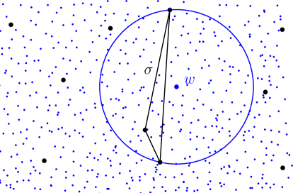
Figure 1: Blue points are the witnesses $W$ and the black points are the landmarks $L$. The simplex $\sigma$ is witnessed by $w$.

Observe that the only predicates involved in the construction of ${\rm Wit}(L,W)$ are (squared) distance comparisons, i.e. polynomials of degree $2$ in the coordinates of the points. This is to be compared with the predicate that decides whether a point lies inside, on or outside the sphere circumscribing a $d$-simplex which is a polynomial of degree $d+2$.

3 Identity of witness and Delaunay complexes

In this section, we make the connection between Delaunay and witness complexes more precise. We start with de Silva’s result [dS08]:

Theorem 3

${\rm Wit}(L,W)\subseteq{\rm Del}(L)$, and if $W=\mathbb{T}^{d}$ then ${\rm Wit}(L,W)={\rm Del}(L)$.

If $L$ is generic, we know that ${\rm Del}(L)$ is embedded in $\mathbb{T}^{d}$ by Delaunay’s theorem. It therefore follows from Theorem 3 that the same is true for ${\rm Wit}(L,W)$. In particular, the dimension of ${\rm Wit}(L,W)$ is at most $d$.

3.1 Identity from protection

When $W$ is not the entire space $\mathbb{T}^{d}$ but a finite set of points, the equality between ${\rm Del}(L)$ and ${\rm Wit}(L,W)$ no longer holds. However, by requiring that the $d$-simplices of ${\rm Del}(L)$ be $\delta$-protected, a property introduced in [BDG13], we are able to recover the inclusion ${\rm Del}(L)\subseteq{\rm Wit}(L,W)$, and establish the equality between the Delaunay complex and the witness complex with a discrete set of witnesses.

Definition 4 ($\delta$-protection)

We say that a simplex $\sigma\subset L$ is $\delta$-protected at $x\in\mathbb{T}^{d}$ if

$$\|x-q\|>\|x-p\|+\delta,\;\;\forall p\in\sigma\;\;\mbox{and}\;\;\forall q\in L\setminus\sigma.$$

We say that ${\rm Del}(L)$ is $\delta$-protected when each Delaunay $d$-simplex of ${\rm Del}(L)$ has a $\delta$-protected Delaunay center. In this sense, $\delta$-protection is in fact a property of the point set and we also say that $L$ is $\delta$-protected. If ${\rm Del}(L)$ is $\delta$-protected for some unspecified $\delta>0$, we say that $L$ is protected (equivalently $L$ is generic). We always assume $\delta<\lambda$ since it is impossible to have a larger $\delta$ if $L$ is a $\lambda$-sample. The following lemma is proved in [BDGO14]. For a subcomplex $K\in{\rm Del}(L)$, we define ${\rm star}(K;{\rm Del}(L))$ as the subcomplex consisting of all the simplices that have at least one vertex in $K$ (note that this definition departs from common usage). We will use $\mathrm{star}^{2}(p)$ as a shorthand for ${\rm star}({\rm star}(p;{\rm Del}(L));{\rm Del}(L))$.

Lemma 5 (Inheritance of protection)

Let $L$ be a $(\lambda,\bar{\mu})$-net and suppose $p\in L$. If every $d$-simplex in $\mathrm{star}^{2}(p)$ is $\delta$-protected, then all simplices in ${\rm star}(p;{\rm Del}(L))$ are at least $\delta^{\prime}$-protected where $\delta^{\prime}=\frac{\bar{\mu}\delta}{4d}$. Specifically, any Delaunay $k$-simplex $\tau$ is $\delta^{\prime}$-protected at a point $z_{\tau}$ which is the barycenter of the circumcenters of a subset of $d-k+1$ $d$-cofaces of $\tau$.

The following lemma is an easy consequence of the previous one.

Lemma 6 (Identity from protection)

Let $L$ be a $(\lambda,\bar{\mu})$-net with $p\in L$. If all the $d$-simplices in $\mathrm{star}^{2}(p)$ are $\delta$-protected and $W$ is an $\varepsilon$-sample for $\mathbb{T}^{d}$ with $\delta\geq\frac{8d\varepsilon}{\bar{\mu}}$, then ${\rm star}(p;{\rm Wit}(L,W))={\rm star}(p;{\rm Del}(L))$.

Proof.

By Theorem 3, we have

$${\rm star}(p;{\rm Wit}(L,W))\subseteq{\rm star}(p;{\rm Del}(L)).$$

We now prove the other inclusion. Let $\sigma$ be a simplex in ${\rm star}(p;{\rm Del}(L))$ and set

$$\delta^{\prime}=\frac{\bar{\mu}\delta}{4d}\geq 2\varepsilon.$$

Let $\tau\subseteq\sigma$ be a face of $\sigma$. Then, by Lemma 5, $\tau$ is $\delta^{\prime}$-protected at a point $z_{\tau}$ such that

1. $\|z_{\tau}-p_{i}\|=\|z_{\tau}-p_{j}\|=r\;\;\;\forall p_{i},p_{j}\in\tau$

2. $\|z_{\tau}-p_{l}\|>r+\delta^{\prime}\;\;\;\forall p_{l}\in L\setminus\tau$

For any $x\in B(z_{\tau},\delta^{\prime}/2)$, any $p_{i}\in\tau$ and any $p_{l}\in L\setminus\tau$, we have

$$\|x-p_{i}\|\leq\|z_{\tau}-p_{i}\|+\|z_{\tau}-x\|\leq r+\frac{\delta^{\prime}}{2}$$

and

$$\|x-p_{l}\|\geq\|z_{\tau}-p_{l}\|-\|x-z_{\tau}\|>r+\delta^{\prime}-\frac{\delta^{\prime}}{2}=r+\frac{\delta^{\prime}}{2}.$$

Hence, $x$ is a witness of $\tau$. Since $\varepsilon\leq\delta^{\prime}/2$, there must be a point $w\in W$ in $B(z_{\tau},\delta^{\prime}/2)$ which witnesses $\tau$. Since this is true for all faces $\tau\subseteq\sigma$, we have $\sigma\in{\rm star}(p;{\rm Wit}(L,W))$. ∎

We end this subsection with a result proved in [BDG13, Lemma 3.13] that will be useful in Section 5. For any vertex $p$ of a simplex $\sigma$, the face oppposite $p$ is the face determined by the other vertices of $\sigma$, and is denoted by $\sigma_{p}$. The altitude of $p$ in $\sigma$ is the distance $D(p,\sigma)=d(p,{\mbox{aff}}(\sigma_{p}))$ from $p$ to the affine hull of $\sigma_{p}$. The altitude $D(\sigma)$ of $\sigma$ is the minimum over all vertices $p$ of $\sigma$ of $D(p,\sigma)$. A poorly-shaped simplex can be characterized by the existence of a relatively small altitude. The thickness of a $j$-simplex $\sigma$ is the dimensionless quantity $\Theta(\sigma)$ that evaluates to $1$ if $j=0$ and to $\frac{D(\sigma)}{j\Delta(\sigma)}$ otherwise, where $\Delta(\sigma)$ denotes the diameter of $\sigma$, i.e. the length of its longest edge.

Lemma 7 (Thickness from protection)

Suppose $\sigma\in{\rm Del}(L)$ is a $d$-simplex with circumradius less than $\lambda$ and shortest edge length greater than or equal to $\bar{\mu}\lambda$. If every $(d-1)$-face of $\sigma$ is also a face of a $\delta$-protected $d$-simplex different from $\sigma$, then the thickness of $\sigma$ satisfies

$$\Theta(\sigma)\geq\frac{\bar{\delta}\,(\bar{\mu}+\bar{\delta})}{8d}.$$

In particular, suppose $p\in L$, where $L$ is a $(\lambda,\bar{\mu})$-net, and every $d$-simplex in $\mathrm{star}^{2}(p)$ is $\delta$-protected, then every $d$-simplex in ${\rm star}(p)$ is $\left(\frac{\bar{\delta}\,\bar{\mu}}{8d}\right)$-thick.

3.2 A combinatorial criterion for identity

The previous result will be useful in our analysis but does not help to compute ${\rm Del}(L)$ from ${\rm Wit}(L,W)$ since the $\delta$-protection assumption requires knowledge of ${\rm Del}(L)$. A more useful result in this context will be given in Lemma 10. Before stating the lemma, we need to introduce some terminology and, in particular, the notion of good links.

Figure 2: Pinched simplicial torus is an example of $2$-pseudo-manifold.

A complex $K$ is a $k$-pseudo-manifold if it is a pure $k$-complex and every $(k-1)$-simplex is the face of exactly two $k$-simplices.

Definition 8 (Good links)

Let $K$ be a complex with vertex set $L\subset\mathbb{T}^{d}$. We say $p\in L$ has a good link if ${\rm link}(p;K)$ is a $(d-1)$-pseudo-manifold. If every $p\in L$ has a good link, we say $K$ has good links.

For our purposes, a simplicial complex $K$ is a triangulation of $\mathbb{T}^{d}$ if it is a $d$-manifold embedded in $\mathbb{T}^{d}$. We observe that a triangulation has good links.

Lemma 9 (Pseudomanifold criterion)

If $K$ is a triangulation of $\mathbb{T}^{d}$ and $J\subseteq K$ has the same vertex set, then $J=K$ if and only if $J$ has good links.

Proof.

Let $L$ be the common vertex set of $K$ and $J$, and let $p$ be a point in $L$. Since $K$ is a triangulation, ${\rm link}(p;K)$ is a simplicial $(d-1)$-sphere, which is a manifold. A $(d-1)$-pseudo-manifold $C_{J}$ cannot be properly contained in a connected $(d-1)$-manifold simplicial complex $C_{K}$, because a $(d-1)$-simplex that does not belong to $C_{J}$ cannot share a $(d-2)$-face with a simplex of $C_{J}$: Every $(d-2)$-simplex of $C_{J}$ is already the face of two $(d-1)$-simplices of $C_{J}$. Since any two $(d-1)$-simplices in $C_{K}$ can be connected by a path confined to the relative interiors of $(d-1)$ and $(d-2)$-simplices, it follows that a $(d-1)$-simplex $\tau\in C_{K}$ must also belong to $C_{J}$. For an arbitrary simplex $\sigma\in C_{K}$, we have that $\sigma$ is a face of a $(d-1)$-simplex $\tau\in C_{K}$, because $C_{K}$ is a pure $(d-1)$-complex (it is a manifold). It follows that $\tau\in C_{J}$ and therefore $\sigma\in C_{J}$.

Therefore, since ${\rm link}(p;J)\subseteq{\rm link}(p;K)$, if $J$ has good links we must have ${\rm link}(p;J)={\rm link}(p;K)$. It follows that ${\rm star}(p;J)={\rm star}(p;K)$ for every $p\in L$, and therefore $J=K$. If $J$ does not have good links it is clearly not equal to $K$, which does. ∎

We can now state the lemma that is at the heart of our algorithm. It follows from Theorem 3, Lemma 9, and Delaunay’s theorem:

Lemma 10 (Identity from good links)

If $L$ is generic and the vertices of ${\rm Wit}(L,W)$ have good links, then ${\rm Wit}(L,W)={\rm Del}(L)$.

4 Turning witness complexes into Delaunay complexes

Let, as before, $L$ be a finite set of landmarks and $W$ a finite set of witnesses. In this section, we intend to use Lemma 10 to construct ${\rm Del}(L^{\prime})$, where $L^{\prime}$ is close to $L$, using only comparisons of (squared) distances. The idea is to first construct the witness complex ${\rm Wit}(L,W)$ which is a subcomplex of ${\rm Del}(L)$ (Theorem 3) that can be computed using only distance comparisons. We then check whether ${\rm Wit}(L,W)={\rm Del}(L)$ using the pseudomanifold criterion (Lemma 9). While there is a vertex $p$ of ${\rm Wit}(L,W)$ that has a bad link (i.e. a link that is not a pseudomanifold), we perturb $p^{\prime}$ and the set of vertices $I(p^{\prime})$, to be exactly defined in Section 4.3 (See Eq. 1) that are responsible for the bad link $L(p^{\prime})={\rm link}(p^{\prime},{\rm Wit}(L^{\prime},W)$, and recompute the witness complex for the perturbed points. We write $L^{\prime}$ for the set of perturbed points at some stage of the algorithm. Each point $p^{\prime}$ is randomly and independently taken from the so-called picking ball $B(p,\rho)$. Upon termination, we have ${\rm Wit}(L^{\prime},W)={\rm Del}(L^{\prime})$. The parameter $\rho$, the radius of the picking balls, must satisfy Eq. (4) to be presented later. The steps are described in more detail in Algorithm 1. The analysis of the algorithm relies on the Moser-Tardos constructive proof of Lovász local lemma.

Algorithm 1 Delaunay triangulation from witness complex

  Input: $L$, $W$, $\rho$, $\lambda$, $\mu$

  while a vertex $p^{\prime}$ of ${\rm Wit}(L^{\prime},W)$ has a bad link do

     perturb $p^{\prime}$ and the points in $I(p^{\prime})$ (defined in Eq. 1)

     update ${\rm Wit}(L^{\prime},W)$

  end while

  Output: ${\rm Wit}(L^{\prime},W)={\rm Del}(L^{\prime})$

4.1 Lovász local lemma

The celebrated Lovász local lemma is a powerful tool to prove the existence of combinatorial objects [AS08]. Let $\mathcal{A}$ be a finite collection of “bad” events in some probability space. The lemma shows that the probability that none of these events occur is positive provided that the individual events occur with a bounded probability and there is limited dependence among them.

Lemma 11 (Lovász local lemma)

Let ${\cal A}=\{A_{1},\,\dots,\,A_{N}\}$ be a finite set of events in some probability space. Suppose that each event $A_{i}$ is independent of all but at most $\Gamma$ of the other events $A_{j}$, and that $\mathsf{Pr}\left[A_{i}\right]\leq\varpi$ for all $1\leq i\leq N$. If

$$\varpi\leq\frac{1}{e(\Gamma+1)}$$

($e$ is the base of the natural logarithm), then

$$\mathsf{Pr}\left[\bigwedge_{i=1}^{N}\neg A_{i}\right]>0.$$

Assume that the events depend on a finite set of mutually independent variables in a probability space. Moser and Tardos [MT10] gave a constructive proof of Lovász lemma leading to a simple and natural algorithm that checks whether some event $A\in{\cal A}$ is violated and randomly picks new values for the random variables on which $A$ depends. We call this a resampling of the event $A$. Moser and Tardos proved that this simple algorithm quickly terminates, providing an assignment of the random variables that avoids all of the events in $\mathcal{A}$. The expected total number of resampling steps is at most $N/\Gamma$.

4.2 Three geometric lemmas

We will be using the following geometric lemmas.

We will need the following technical result to prove Lemma 15.

Lemma 12

If $L$ is a $\lambda$-sample of $\mathbb{T}^{d}$, the circumradius $R_{\sigma}$ of any simplex $\sigma$ in ${\rm Wit}(L,W)$ is less than $\lambda$. The witnesses of $\sigma$ are at a distance less than $\lambda$ from the closest vertex of $\sigma$ and at a distance less than $3\lambda$ from any vertex of $\sigma$.

Proof.

By Theorem 3, $\sigma$ is a simplex of ${\rm Del}(L)$ and, since $L$ is a $\lambda$-sample of $\mathbb{T}^{d}$, the circumradius $R_{\sigma}$ is less than $\lambda$. Let $w$ be a witness of $\sigma$ and $q$ the vertex of $\sigma$ closest to $w$. Since $L$ is a $\lambda$-sample, $\|w-q\|<\lambda$. The diameter of $\sigma$ is thus at most $2R_{\sigma}<2\lambda$, and $\|w-p\|<3\lambda$ for any vertex $p\in\sigma$. ∎

Lemma 13

If $L$ is a $(\lambda,\bar{\mu})$-net of $\mathbb{T}^{d}$ and $4\bar{\rho}<\bar{\mu}$, then $L^{\prime}$ is an $(\lambda^{\prime},\bar{\mu}^{\prime})$-net, where

$$\lambda^{\prime}=\lambda(1+\bar{\rho})\;\;\mbox{and}\;\;\bar{\mu}^{\prime}=\frac{\bar{\mu}-2\bar{\rho}}{1+\bar{\rho}}\geq\frac{\bar{\mu}}{3}.$$

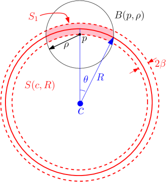
Figure 3: For Lemma 14.

Lemma 14

(See [BDG14, Lemma 5.2]) Let $S(c,R)$ be a hypersphere of $\mathbb{R}^{d}$ of radius $R$ centered at $c$ and $T_{\delta}$ the spherical shell $T_{\delta}=B(c,R+\delta)\setminus B(c,R)$. Let, in addition, $B_{\rho}$ denote any $d$-ball of radius $\rho<R$. We have

$${\rm vol}_{d}(T_{\delta}\cap B_{\rho})\leq U_{d-1}\left(\frac{\pi}{2}\rho\right)^{d-1}\delta,$$

where $U_{d-1}$ denotes the volume of a Euclidean $(d-1)$-ball with unit radius.

4.3 Correctness of the algorithm

We first bound the density radius $\lambda^{\prime}$ and the sparsity ratio $\bar{\mu}^{\prime}$ of any perturbed point set $L^{\prime}$. We will write $\rho=\bar{\rho}\lambda$ and $\mu=\bar{\mu}\lambda$, and assume $\bar{\rho}<\bar{\mu}/4$.

We refer to the terminology of the Lovász local lemma. Our variables are the points of $L^{\prime}$ which are randomly and independently taken from the picking balls $B(p,\rho)$, $p\in L$.

The events are associated to points of $L^{\prime}$, the vertices of ${\rm Wit}(L^{\prime},W)$. We say that an event happens at $p^{\prime}\in L$ when the link $L(p^{\prime})$ of $p^{\prime}$ in ${\rm Wit}(L^{\prime},W)$ is not good, i.e., is not a pseudomanifold. We know from Lemma 6 that if $p^{\prime}$ is a vertex of ${\rm Wit}(L^{\prime},W)$ and $L(p^{\prime})$ is not good, then there must exist a $d$-simplex in $\mathrm{star}^{2}(p^{\prime})$ that is not $\delta$-protected for $\delta=8d\varepsilon/\bar{\mu}$. We will denote by

• $I_{1}(p^{\prime}):$ the set of points of $L^{\prime}$ that can be in $\mathrm{star}^{2}(p^{\prime})={\rm star}({\rm star}(p^{\prime};{\rm Del}(L^{\prime});{\rm Del}(L^{\prime}))$

• $I_{2}(p^{\prime}):$ the set of points of $L^{\prime}$ that can violate the $\delta$-protected zone $Z_{\delta}(\sigma^{\prime})=B(c_{\sigma},R_{\sigma}+\delta)\setminus B(c_{\sigma},R_{\sigma})$ for some $d$-simplex $\sigma^{\prime}$ in $\mathrm{star}^{2}(p^{\prime})$

• $I(p^{\prime}):$ Since computing $I_{1}(p^{\prime})$ and $I_{2}(p^{\prime})$ exactly is difficult, we will rather compute the set

  $$I(p^{\prime})=\left\{q^{\prime}\;:\;q\in L\cap B(p,R)\;\mbox{where}\;R=5\lambda+\frac{3\bar{\mu}\lambda}{2}\right\}.$$ (1)

  Using triangle inequality, Lemma 13, and the facts that $\bar{\rho}<\bar{\mu}/4$ and $\delta\leq\lambda$, we can show that

  $$I(p^{\prime})\supseteq\tilde{I}_{1}(p^{\prime})\cup\tilde{I}_{2}(p^{\prime}),$$

  where $\tilde{I}_{i}(p^{\prime})$ is the set of points in $L$ that correspond to points in $I_{i}(p^{\prime})\subset L^{\prime}$.

• $S(p^{\prime}):$ the set of $d$-simplices with vertices in $I_{1}(p^{\prime})$ that can belong to $\mathrm{star}^{2}(p^{\prime})$

The probability $\varpi_{1}(p^{\prime})$ that $L(p^{\prime})$ is not good is at most the probability $\varpi_{2}(p^{\prime})$ that one of the simplices of $S(p^{\prime})$, say $\sigma^{\prime}$, has its $\delta$-protecting zone $Z_{\delta}(\sigma^{\prime})$ violated by some point of $L^{\prime}$. Write $\varpi_{3}(q^{\prime},\sigma^{\prime})$ for the probability that $q^{\prime}$ belongs to the $\delta$-protection zone of the $d$-simplex $\sigma^{\prime}$. We have

$$\varpi_{1}(p^{\prime})\leq\varpi_{2}(p^{\prime})\leq\sum_{q^{\prime}\in I_{2}(p^{\prime})}\,\sum_{\sigma^{\prime}\in S(p^{\prime})}\varpi_{3}(q^{\prime},\sigma^{\prime})$$ (2)

The following lemmas provide upper bounds on $|I(p^{\prime})|$, $|S(p^{\prime})|$, $\Gamma$ and $\varpi_{3}(q^{\prime},\sigma^{\prime})$.

Lemma 15

$|I(p^{\prime})|\leq I=\left(\frac{14}{\bar{\mu}}\right)^{d}$ and $|S(p^{\prime})|\leq K{=}\frac{I^{d+1}}{(d+1)!}$.

Proof.

Since any two points in $L$ are at least $\bar{\mu}\lambda$ apart, a volume argument then gives the announced bound. Referring to (1) we have

$$|I(p^{\prime})|\leq\left(\frac{5\lambda+\frac{3\bar{\mu}\lambda}{2}+\frac{\bar{\mu}\lambda}{2}}{\frac{\bar{\mu}\,\lambda}{2}}\right)^{d}\leq\left(4+\frac{10}{\bar{\mu}}\right)^{d}\leq\left(\frac{14}{\bar{\mu}}\right)^{d}.$$

We thus have

$$|S(p^{\prime})|\leq\left(\begin{array}[]{c}I\\ d+1\end{array}\right)\leq\frac{I^{d+1}}{(d+1)!}.$$

∎

Lemma 16

An event is independent of all but at most $\Gamma=\left(\frac{27}{\bar{\mu}}\right)^{d}$ other events.

Proof.

Two events $p^{\prime}$ and $q^{\prime}$ are independent if $I(p^{\prime})\cap I(q^{\prime})=\emptyset$. Referring to $R$ defined in (1), this implies $p^{\prime}$ and $q^{\prime}$ are independent if $\|p-q\|<2R=10\lambda+3\bar{\mu}\lambda$. Hence an upper bound on the number of events that may not be independent from the event at $p^{\prime}$ is given by a volume argument as in the proof of Lemma 15. Here we count points since the events are associated to points:

$$\left(\frac{10\lambda+3\bar{\mu}\lambda+\frac{\bar{\mu}\,\lambda}{2}}{\frac{\bar{\mu}\,\lambda}{2}}\right)^{d}\leq\left(7+\frac{20}{\bar{\mu}}\right)^{d}\leq\left(\frac{27}{\bar{\mu}}\right)^{d}\stackrel{{\scriptstyle{\rm def}}}{{=}}\Gamma.$$

∎

Lemma 17

$\varpi_{3}(q^{\prime},\sigma^{\prime})\leq 2\pi^{d-1}\frac{\delta}{\rho}$.

Proof.

The volume of Euclidean $d$-ball with unit radius will be denoted by $U_{d}$. The probability $\varpi_{3}(q^{\prime},\sigma^{\prime})$ is the ratio between the volume of the portion of the picking region that is in the spherical shell $B(c_{\sigma^{\prime}},R_{\sigma^{\prime}}+\delta)\setminus B(c_{\sigma^{\prime}},R_{\sigma^{\prime}})$ and the volume of the picking region. Hence, using [BDG14, Lem. 5.2] and the crude bound $\frac{U_{d-1}}{U_{d}}\leq 2^{d}$, we obtain

$$\varpi_{3}(q^{\prime},\sigma^{\prime})\leq\frac{U_{d-1}\,(\frac{\pi}{2}\,\rho)^{d-1}\,\delta}{U_{d}\,\rho^{d}}\leq 2\pi^{d-1}\,\frac{\delta}{\rho}.$$

∎

Using Eq. (2), and Lemmas 15 and 17, we conclude that

$$\varpi_{1}(p^{\prime})\leq 2\pi^{d-1}\,I\,K\,\frac{\delta}{\rho}.$$

An event depends on at most $\Gamma$ other events. Hence, to apply the Lovász Local Lemma 11, it remains to ensure that $\varpi_{1}(p^{\prime})\leq\frac{1}{(e(\Gamma+1))}$. In addition, we also need that $\delta\geq\frac{8d\varepsilon}{\bar{\mu}^{\prime}}$ to be able to apply Lemma 6. We thefore need to satisfy the following inequality:

$$\frac{8d\varepsilon}{\bar{\mu}^{\prime}}\leq\delta\leq J\rho\;\;\mbox{where}\;\;J^{-1}\stackrel{{\scriptstyle{\rm def}}}{{=}}2e\pi^{d-1}IK(\Gamma+1)=\left(\frac{2}{\bar{\mu}}\right)^{O(d^{2})}$$ (3)

Observe that $I$, $K$, $\Gamma$ and $J$ depend only on $\bar{\mu}$ and $d$. We conclude that the conditions of the Lovász local lemma hold if the parameter $\rho$ satisfies

$$\frac{\mu}{4}\geq\rho\geq\frac{24d\varepsilon}{\bar{\mu}J}$$ (4)

Hence, if $\varepsilon$ is sufficiently small, we can fix $\rho$ so that Eq. (4) holds. The algorithm is then guaranteed to terminate. By Lemma 10, the output is ${\rm Del}(L^{\prime})$.

It follows from Moser-Tardos theorem that the expected number of times the "while-loop" in Algorithm 1 runs is $O\left(\frac{|L|}{\Gamma}\right)$ and since $|I(p^{\prime})|\leq I$, we get that the number of point perturbations performed by Algorithm 1 is $O\left(\frac{I\,|L|}{\Gamma}\right)=O(|L|)$ on expectation, where the constant in the $O$ depends only on $d$ and not on the sampling parameters $\lambda$ or $\mu$. We sum up the results of this section in

Theorem 18

Under Eq. (4), Algorithm 1 terminates and outputs the Delaunay triangulation of some set $L^{\prime}$ whose distance to $L$ is at most $\rho$. The number of point perturbations performed by the algorithm is $O\left(|L|\right)$.

5 Sublinear algorithm

When the set $L^{\prime}$ is generic, $K={\rm Wit}(L^{\prime},W)$ is embedded in $\mathbb{T}^{d}$ and is therefore $d$-dimensional. It is well known that the $d$-skeleton of ${\rm Wit}(L^{\prime},W)$ can be computed in time $O((|W|+|K|)\log|L^{\prime}|)$ using only distance comparisons [BM14]. Although easy and general, this construction is not efficient when $W$ is large.

In this section, we show how to implement an algorithm with execution time sublinear in $|W|$. We will assume that the points of $W$ are located at the centers of a grid, which is no real loss of generality. The idea is to restrict our attention to a subset of $W$, namely the set of full-leaf-points introduced in Section 5.2. These are points that may be close to the circumcentre of some $d$-simplex. A crucial observation is that if a $d$-simplex has a bounded thickness, then we can efficiently compute a bound on the number of its full-leaf-points. This observation will also allow us to guarantee some protection (and therefore thickness) on the output simplices, as stated in Theorem 26 below.

The approach is based on the relaxed Delaunay complex, which is related to the witness complex, and was also introduced by de Silva [dS08]. We first introduce this, and the structural observations on which the algorithm is based.

5.1 The relaxed Delaunay complex

The basic idea used to get an algorithm sublinear in $|W|$ is to choose witnesses for $d$-simplices that are close to being circumcentres for these simplices. With this approach, we can in fact avoid looking for witnesses of the lower dimensional simplices. The complex that we will be computing is a subcomplex of a relaxed Delaunay complex:

Definition 19 (Relaxed Delaunay complex)

Let $\sigma\subset L^{\prime}$ be a simplex. An $\alpha$-center of $\sigma$ is any point $x\in\mathbb{T}^{d}$ such that

$$\|x-p\|\leq\|x-q\|+\alpha,\;\;\forall\,p,\,q\in\sigma.$$

We say that $x$ is an $\alpha$-Delaunay center of $\sigma$ if

$$\|x-p\|\leq\|x-q\|+\alpha,\;\;\forall p\in\sigma\;\mbox{and}\;\forall q\in L^{\prime}.$$

The set of simplices that have an $\alpha$-Delaunay centre in $W$ is a simplicial complex, called the $\alpha$-relaxed Delaunay complex, and is denoted ${\rm Del}^{\alpha}(L^{\prime},W)$.

We say $w\in W$ is an $\alpha$-witness for $\sigma\subset L^{\prime}$ if

$$\|w-p\|\leq\|w-q\|+\alpha,\;\;\forall p\in\sigma\;\;\mbox{and}\;\;\forall q\in L^{\prime}\setminus\sigma.$$

We observe that $w\in W$ is an $\alpha$-Delaunay center if and only if it is an $\alpha$-center and also an $\alpha$-witness.

Lemma 20

The distance between an $\alpha$-Delaunay center for $\sigma\in{\rm Del}^{\alpha}(L^{\prime},W)$ and the farthest vertex in $\sigma$ is less than $\lambda^{\prime}+\alpha$. In particular, $\Delta_{\sigma}<2\lambda^{\prime}+2\alpha$.

If $\tau\in{\rm Del}(L^{\prime})$ and $c$ is a Delaunay center of $\tau$, then any point in $B(c,r)$ is a $2r$-Delaunay centre for $\tau$. Thus ${\rm Del}(L^{\prime})\subseteq{\rm Del}^{2\varepsilon}(L^{\prime},W)$.

If, for some $\delta\geq 0$, all the $d$-simplices in ${\rm Del}^{\alpha}(L^{\prime},W)$ have a $\delta$-protected circumcentre, then we have that ${\rm Del}^{\alpha}(L^{\prime},W)\subseteq{\rm Del}(L^{\prime})$, and with $\alpha\geq 2\varepsilon$, it follows (Lemma 20) that ${\rm Del}^{\alpha}(L^{\prime},W)={\rm Del}(L^{\prime})$, and ${\rm Del}(L^{\prime})$ is itself $\delta$-protected and has good links.

Reviewing the analysis of the Moser-Tardos algorithm of Section 4.3, we observe that the exact same estimate of $\varpi_{2}(p^{\prime})$ that serves as an upper bound on the probability that one of the simplices in $\mathrm{star}^{2}(p^{\prime},{\rm Del}(L^{\prime}))$ is not $\delta$-protected at its circumcenter, also serves as an upper bound on the probability that one of the simplices in $\mathrm{star}^{2}(p^{\prime},{\rm Del}^{\alpha}(L^{\prime},\mathbb{T}^{d}))$ is not $\delta$-protected at its circumcenter, provided that $4\alpha+\delta\leq\lambda^{\prime}$ (using the diameter bound of $2\lambda^{\prime}+2\alpha$ from Lemma 20), which we will assume from now on. We can therefore modify Algorithm 1 by replacing ${\rm Wit}(L^{\prime},W)$ by ${\rm Del}^{\alpha}(L^{\prime},W)$.

We now describe how to improve this algorithm to make it efficient. For our purposes it will be sufficient to set $\alpha=2\varepsilon$. In order to obtain an algorithm sublinear in $|W|$, we will not compute the full ${\rm Del}^{2\varepsilon}(L^{\prime},W)$ but only a subcomplex we call ${\rm Del}^{2\varepsilon}_{0}(L^{\prime},W)$. The exact definition of ${\rm Del}^{2\varepsilon}_{0}(L^{\prime},W)$ will be given in Section 5.3, but the idea is to only consider $d$-simplices that show the properties of being $\Theta_{0}$-thick for some parameter $\Theta_{0}$ to be defined later (Eq. 5 and 6). This will allow us to restrict our attention to points of $W$ that lie near the circumcentre. As explained in Section 5.3, this is done without explicitly computing thickness or circumcentres.

As will be shown in Section 5.4 (Lemma 24), the modification of Algorithm 1 that computes ${\rm Del}^{2\varepsilon}_{0}(L^{\prime},W)$ instead of ${\rm Wit}(L^{\prime},W)$ will terminate and output a complex ${\rm Del}^{2\varepsilon}_{0}(L^{\prime},W)$ with good links. However, this is not sufficient to guarantee that the output is correct, i.e., that ${\rm Del}^{2\varepsilon}(L^{\prime},W)={\rm Del}(L^{\prime})$. In order to obtain this guarantee, we insert an extra procedure check(), which, without affecting the termination guarantee, will ensure that the simplices of ${\rm Del}^{2\varepsilon}_{0}(L^{\prime},W)$ have $\delta^{*}$-protected circumcenters for a positive $\delta^{*}$. It follows that ${\rm Del}^{2\varepsilon}_{0}(L^{\prime},W)\subseteq{\rm Del}(L^{\prime})$ and, by Lemma 9, that ${\rm Del}^{2\varepsilon}_{0}(L^{\prime},W)={\rm Del}(L^{\prime})$. The modification of Algorithm 1 that we will use is outlined in Algorithm 2.

Algorithm 2 Protected Delaunay triangulation from ${\rm Del}^{2\varepsilon}_{0}(L^{\prime},W)$

  input: $L$, $W$, $\rho$, $\varepsilon$, $\lambda$, $\mu$

  $L^{\prime}\leftarrow L$

  compute: ${\rm Del}^{2\varepsilon}_{0}(L^{\prime},W)$

  while a vertex $p^{\prime}$ of ${\rm Del}^{2\varepsilon}_{0}(L^{\prime},W)$ has a bad link or check$(p^{\prime})=\mathrm{FALSE}$ do

     perturb $p^{\prime}$ and the points in $I(p^{\prime})$  ($I(p^{\prime})$ is defined in Section 4.3.)

     update ${\rm Del}^{2\varepsilon}_{0}(L^{\prime},W)$

  end while

  output: ${\rm Del}^{2\varepsilon}_{0}(L^{\prime},W)={\rm Del}(L^{\prime})$ with $\delta^{*}$ protection (See Lemma 25)

We describe the details of computing ${\rm Del}^{2\varepsilon}_{0}(L^{\prime},W)$ and of the check() procedure in the following subsections.

5.2 Computing relaxed Delaunay centers

We observe that the $\alpha$-Delaunay centers of a $d$-simplex $\sigma$ are close to the circumcenter of $\sigma$, provided that $\sigma$ has a bounded thickness:

Lemma 21 (Clustered $\alpha$-Delaunay centers)

Assume that $L^{\prime}$ is a $(\lambda^{\prime},\bar{\mu}^{\prime})$-sample. Let $\sigma$ be a non degenerate $d$-simplex, and let $x$ be an $\alpha$-center for $\sigma$ at distance at most $C\lambda^{\prime}$ from the vertices of $\sigma$, for some constant $C>0$. Then $x$ is at distance at most $\frac{C\alpha}{\Theta(\sigma)\bar{\mu}^{\prime}}$ from the circumcenter $c_{\sigma}$ of $\sigma$. In particular, if $x$ is an $\alpha$-Delaunay center for $\sigma$, then

$$\|c_{\sigma}-x\|<\frac{2\alpha}{\Theta(\sigma)\bar{\mu}^{\prime}}.$$

Proof.

Using [BDG13, Lemma 4.3] and $\Delta(\sigma)\geq\bar{\mu}^{\prime}\lambda^{\prime}$, we get

$$\|w_{\sigma}-c_{\sigma}\|\leq\frac{C\lambda^{\prime}\alpha}{\Theta(\sigma)\Delta(\sigma)}\leq\frac{C\alpha}{\Theta(\sigma)\bar{\mu}^{\prime}}.$$

The second assertion follows from this together with Lemma 20, and the assumption that $\alpha<\lambda^{\prime}$. ∎

It follows from Lemma 21 that $\alpha$-Delaunay centers are close to all the bisecting hyperplanes

$$H_{pq}=\{x\in\mathbb{R}^{d}\,|\,\|x-p\|=\|x-q\|,\,\,p,q\in\sigma\}.$$

The next simple lemma asserts a kind of qualitative converse:

Lemma 22

Let $\sigma$ be a $d$-simplex and $H_{pq}$ be the bisecting hyperplane of $p$ and $q$. A point $x$ that satisfies $d(x,H_{pq})\leq\alpha$, for any $p,q\in\sigma$ is a $2\alpha$-center of $\sigma$.

Let $\sigma$ be a $d$-simplex of ${\rm Del}^{\alpha}(L^{\prime},W)$ and let $\bar{\Omega}$ be the smallest box with edges parallel to the coordinate axes that contains $\sigma$. Then the edges of $\bar{\Omega}$ have length at most $2\lambda^{\prime}+2\alpha$ (Lemma 20). Any $\alpha$-Delaunay center for $\sigma$ is at a distance at most $\lambda^{\prime}+\alpha$ from $\bar{\Omega}$. Therefore all the $\alpha$-Delaunay centers for $\sigma$ lie in an axis-aligned hypercube $\Omega$ with the same center as $\bar{\Omega}$ and with side length at most $4\lambda^{\prime}+4\alpha<5\lambda^{\prime}$. Observe that the diameter (diagonal) $z$ of $\Omega$ is at most $5\lambda^{\prime}\sqrt{d}$.

Our strategy is to first compute the $\alpha$-centers of $\sigma$ that belong to $\Omega\cap W$ and then to determine which ones are $\alpha$-witnesses for $\sigma$. Deciding if an $\alpha$-center is an $\alpha$-witness for $\sigma$ can be done in constant time since $L^{\prime}$ is a $(\lambda^{\prime},\bar{\mu}^{\prime})$-net and $\Delta_{\sigma}\leq 2\lambda^{\prime}+2\alpha$ (Lemma 20).

We take $\alpha=2\varepsilon$. To compute the $2\varepsilon$-Delaunay centers of $\sigma$, we will use a pyramid data structure. The pyramid consists of at most $\log\frac{z}{\varepsilon}$ levels. Each level $h>0$ is a grid of resolution $2^{-h}z$. The grid at level $0$ consists of the single cell, $\Omega$. Each node of the pyramid is associated to a cell of a grid. The children of a node $\nu$ correspond to a subdivision into $2^{d}$ subcells (of the same size) of the cell associated to $\nu$. The leaves are associated to the cells of the finest grid whose cells have diameter $\varepsilon$.

A node of the pyramid that is intersected by all the bisecting hyperplanes of $\sigma$ will be called a full node or, equivalently, a full cell. By our definition of $W$, a cell of the finest grid contains an element of $W$ at its centre. The full-leaf-points are the elements of $W$ associated to full cells at the finest level. By Lemma 22, the full-leaf-points are $2\varepsilon$-centers for $\sigma$. In order to identify the full-leaf cells, we traverse the full nodes of the pyramid starting from the root. Note that to decide if a cell is full, we only have to decide if two corners of a cell are on opposite sides of a bisecting hyperplane, which reduces to evaluating a polynomial of degree 2 in the input variables.

We will compute a bound $n_{\sigma}(\varepsilon)$ on the number of full cells in the pyramid. Consider a level in the pyramid and the associated grid $G_{\omega}$ whose cells have diameter $\omega$. Any point in a full cell of $G_{\omega}$ is at distance $\omega$ from the bisecting hyperplanes of $\sigma$ and so, by Lemma 22, is a $2\omega$-center for $\sigma$. By construction of $\Omega$, the distance between a point $w\in\Omega$ and a vertex $p\in\sigma$ is bounded by

$$\|w-p\|\leq(3\lambda^{\prime}+3\alpha)\sqrt{d}<4\lambda^{\prime}\sqrt{d}.$$

Therefore, it follows from Lemma 21 that all the full cells of $G_{\omega}$ are contained in a ball of radius $\frac{4\sqrt{d}\omega}{\Theta(\sigma)\bar{\mu}^{\prime}}$ centered at $c_{\sigma}$. Letting $C$ be a hypercube with the dimensions of a cell in $G_{\omega}$, a volume argument gives a bound on $n_{\omega}$, the number of full cells in $G_{\omega}$:

$$n_{\omega}\leq\frac{{\rm vol}(B)}{{\rm vol}(C)}=U_{d}\left(\frac{4\sqrt{d}\omega}{\Theta(\sigma)\bar{\mu}^{\prime}}\right)^{d}\left(\frac{\sqrt{d}}{\omega}\right)^{d}=U_{d}\left(\frac{4d}{\Theta(\sigma)\bar{\mu}^{\prime}}\right)^{d},$$

where $U_{d}$ is the volume of the Euclidean ball of unit radius.

Observe that $n_{\omega}$ does not depend on $\omega$. Hence we can apply this bound to all levels of the pyramid, from the root level to the leaves level. Since there are at most $\log\frac{5\lambda^{\prime}\sqrt{d}}{\varepsilon}$ levels, we conclude with the following lemma:

Lemma 23

The number of full cells is less than

$$n_{\sigma}(\varepsilon)=\frac{U_{d}(4d)^{d}}{(\Theta(\sigma)\bar{\mu}^{\prime})^{d}}{\log\frac{5\sqrt{d}\lambda^{\prime}}{\varepsilon}}.$$

$n_{\sigma}(\varepsilon)$ is also a bound on the time to compute the full cells.

5.3 Construction of ${\rm Del}^{2\varepsilon}_{0}(L^{\prime},W)$

By Lemma 20, all the simplices incident to a vertex $p^{\prime}$ of ${\rm Del}^{2\varepsilon}(L^{\prime})$ are contained in $N(p^{\prime})=L^{\prime}\cap B(p^{\prime},2\lambda^{\prime}+4\varepsilon)$, and it follows from the fact that $L^{\prime}$ is a $(\lambda^{\prime},\bar{\mu}^{\prime})$-net that

$$|N(p^{\prime})|\leq\frac{2^{O(d)}}{(\bar{\mu}^{\prime})^{d}}.$$

In the first step of the algorithm, we compute, for each $p^{\prime}\in L^{\prime}$, the set $N(p^{\prime})$, and the set of $d$-simplices

$$C_{d}(p^{\prime})=\left\{\sigma=\{p^{\prime}\}\cup\tilde{\sigma}:\leavevmode\nobreak\ \mbox{$|\tilde{\sigma}|=d$ and $\tilde{\sigma}\subset N(p^{\prime})\setminus\{p^{\prime}\}$}\right\}.$$

Observe that

$$|C_{d}(p^{\prime})|=\binom{|N(p^{\prime})|}{d}=\frac{2^{O(d^{2})}}{(\bar{\mu}^{\prime})^{d^{2}}}.$$

We then extract from $C_{d}(p^{\prime})$ a subset $WC_{d}(p^{\prime})$ of simplices that have a full-leaf-point that is a $2\varepsilon$-Delaunay center, and have a number of full cells less than or equal to

$$n_{0}(\varepsilon)\stackrel{{\scriptstyle\rm def}}{{=}}U_{d}\left(\frac{4d}{\Theta_{0}\bar{\mu}^{\prime}}\right)^{d}\log\frac{5\sqrt{d}\lambda^{\prime}}{\varepsilon}.$$

This is done by applying the algorithm of Section 5.2 with a twist. As soon as a $d$-simplex appears to have more than $n_{0}(\varepsilon)$ full cells, we stop considering that simplex. The union of the sets $WC_{d}(p^{\prime})$ for all $p^{\prime}\in L^{\prime}$ is a subcomplex of ${\rm Del}^{2\varepsilon}(L^{\prime})$ called ${\rm Del}^{2\varepsilon}_{0}(L^{\prime},W)$. It contains every $d$-simplex $\sigma$ in ${\rm Del}^{2\varepsilon}(L^{\prime},W)$ that has a $2\varepsilon$-Delaunay center in $W$ at a distance less than $\varepsilon$ from its actual circumcenter, and satisfies the thickness criterion $\Theta(\sigma)\geq\Theta_{0}$. Note, however, that we do not claim that every simplex that has at most $n_{0}(\varepsilon)$ full cells is $\Theta_{0}$-thick. Algorithm 3 describes the construction of ${\rm Del}^{2\varepsilon}_{0}(L,W)$. As noted above, $|N(p^{\prime})|=\frac{2^{O(d)}}{(\bar{\mu}^{\prime})^{d}}$ for any $p^{\prime}\in L^{\prime}$, and all the $N(p^{\prime})$ can be computed in $O(|L^{\prime}|^{2})$ time by a brute fore method. But assuming we have access to “universal hash functions” then we can use “grid method” described in [HP11, Chapter 1] with the sparsity condition of $L$ to get the complexity down to

$$\frac{2^{O(d)}|L^{\prime}|}{(\bar{\mu}^{\prime})^{d}}.$$

Using the facts that $\lambda^{\prime}<2\lambda$ and $\bar{\mu}^{\prime}\geq\frac{\bar{\mu}}{3}$, see Lemma 13, we conclude that the total complexity of the algorithm is

$$O\left(\frac{|L|}{\Theta^{d}_{0}\,\bar{\mu}^{d^{2}+d}}\,\log\frac{\lambda}{\varepsilon}\right)$$

and is therefore sublinear in $|W|$. The constant in $O$ depends only on $d$.

Algorithm 3 Construction of ${\rm Del}^{2\varepsilon}_{0}(L^{\prime},W)$

  input: a $(\lambda^{\prime},\bar{\mu}^{\prime})$-net $L^{\prime}$, a grid $W$ of resolution $\varepsilon$, and $\Theta_{0}$ (defined in Eq. 5 and 6))

   $\Sigma:=\emptyset$

  for each $p^{\prime}\in L^{\prime}$ do

      compute the sets $N(p^{\prime})=L^{\prime}\cap B(p^{\prime},2\lambda^{\prime}+4\varepsilon)$ and $C_{d}(p^{\prime})$

  end for

  for each $p^{\prime}\in L^{\prime}$ do

     for each $d$-simplex $\sigma\in C_{d}(p^{\prime})$ do

        // find the simplices in $C_{d}(p^{\prime})$ that are in $WC_{d}(p^{\prime})$

        if $\sigma$ has a full-leaf-point that is a $2\varepsilon$-Delaunay center and $n_{\sigma}(\varepsilon)\leq n_{0}(\varepsilon)$ then

           add $\sigma$ to $\Sigma$

        end if

     end for

  end for

  output: $\Sigma$ the set of $d$-simplices of ${\rm Del}^{2\varepsilon}_{0}(L^{\prime},W)$

5.4 Correctness of the algorithm

We will need the following lemma which is an analog of Lemma 6. The lemma also bounds $\Theta_{0}$. Its proof follows directly from Lemma 7, and the observation that any simplex with a protected circumcentre is a Delaunay simplex.

Lemma 24

Suppose that the $d$-simplices in ${\rm Del}(L^{\prime})$ are $\delta$-protected at their circumcenters, with $\delta=\bar{\delta}\lambda^{\prime}$. If $0<\Theta_{0}\leq\frac{\bar{\delta}\bar{\mu}}{24d}$, then ${\rm Del}(L^{\prime})\subseteq{\rm Del}^{2\varepsilon}_{0}(L^{\prime},W)$ and if, in addition, every $d$-simplex of ${\rm Del}^{2\varepsilon}_{0}(L^{\prime},W)$ has a protected circumcenter, then ${\rm Del}^{2\varepsilon}_{0}(L^{\prime},W)={\rm Del}(L^{\prime})$.

We first show that Algorithm 2 terminates if we deactivate the call to procedure check(). As discussed after Lemma 20, the analysis of Section 4.3 implies that the perturbations of Algorithm 2 can be expected to produce a point set $L^{\prime}$ for which all the $d$-simplices in ${\rm Del}^{2\varepsilon}(L^{\prime},\mathbb{T}^{d})$ have a $\delta$-protected circumcentre. Since this complex includes both ${\rm Del}(L^{\prime})$ and ${\rm Del}^{2\varepsilon}_{0}(L^{\prime},W)$, Lemma 24 shows that we can expect the algorithm to terminate with the condition that ${\rm Del}^{2\varepsilon}_{0}(L^{\prime},W)$ has good links.

We now examine procedure check() and show that it does not affect the termination guarantee. By Lemma 7, if ${\rm Del}(L^{\prime})$ is $\delta$-protected, then any $\sigma\in{\rm Del}(L^{\prime})$ satisfies

$$\Theta(\sigma)\geq\frac{\bar{\delta}\bar{\mu}^{\prime}}{8d}\geq\frac{\bar{\delta}\bar{\mu}}{24d}\stackrel{{\scriptstyle\text{def}}}{{=}}\Theta_{0}.$$ (5)

Consider now $\sigma\in{\rm Del}^{2\varepsilon}_{0}(L^{\prime},W)$. Since the full leaves of the pyramid data-structure for $\sigma$ are composed entirely of $2\varepsilon$-centres at a distance less than $4\sqrt{d}\lambda^{\prime}$ from any vertex of $\sigma$, Lemma 21 implies that, if $\sigma$ is $\Theta_{0}$-thick, then

$$\|x-c_{\sigma}\|\leq\frac{8\sqrt{d}\varepsilon}{\Theta_{0}\bar{\mu}^{\prime}}.$$

This means that we can restrict our definition of ${\rm Del}^{2\varepsilon}_{0}(L^{\prime},W)$ to include only simplices for which the set of full leaves has diameter less than $\frac{16\sqrt{d}\varepsilon}{\Theta_{0}\bar{\mu}^{\prime}}$. Further, we observe that if $\sigma$ is $\delta$-protected at its circumcentre, then it will have a $(\delta-2\varepsilon)$-protected full-leaf-point; this follows from the triangle inequality. The check() procedure described in Algorithm 4 ensures that all the simplices in ${\rm Del}^{2\varepsilon}_{0}(L^{\prime},W)$ have these two properties. It follows from the discussion above that activating procedure check() does not affect the termination guarantee.

Algorithm 4 procedure check$(p^{\prime})$

  if  all $d$-simplices $\sigma\in{\rm star}(p^{\prime};{\rm Del}^{2\varepsilon}_{0}(L^{\prime},W))$ satisfy

  1. The diameter of the full leaves is at most $\frac{16\sqrt{d}\varepsilon}{\Theta_{0}\bar{\mu}^{\prime}}$.

  2. There is a $(\delta-2\varepsilon)$-protected full-leaf-point  then

      check$(p^{\prime})=\mathrm{TRUE}$

  else

     check$(p^{\prime})=\mathrm{FALSE}$

  end if

The fact that the algorithm terminates yields ${\rm Del}^{2\varepsilon}_{0}(L^{\prime},W)$ with good links. In order to apply Lemma 24 to guarantee that ${\rm Del}^{2\varepsilon}_{0}(L^{\prime},W)={\rm Del}(L^{\prime})$, we need to guarantee that the simplices of ${\rm Del}^{2\varepsilon}_{0}(L^{\prime},W)$ are protected. The analysis of the Moser-Tardos algorithm in Section 4.3 provides a possible $\delta$-protection with

$$\delta=J\rho,$$ (6)

where $J$ is defined in Eq. (3). However, we cannot guarantee that this protection is actually obtained. The following lemma shows that if the perturbation $\rho$ (and consequently $\delta$) is sufficiently large, then the output point set will be $\delta^{*}$-protected for a positive $\delta^{*}$.

Lemma 25

The $d$-simplices in ${\rm Del}^{2\varepsilon}_{0}(L^{\prime},W)$ produced by Algorithm 2 are $\delta^{*}$-protected, with

$$\delta^{*}=\delta-\left(\frac{34\sqrt{d}}{\Theta_{0}\bar{\mu}^{\prime}}\right)\varepsilon,$$

where $\delta=J\rho$.

of Lemma 25.

Let $\sigma\in{\rm Del}^{2\varepsilon}_{0}(L^{\prime},W)$ be a $d$-simplex produced by Algorithm 2, and let $w$ be the full-leaf-point for $\sigma$ found by the check() procedure. Since $c_{\sigma}$ is located in a full leaf-node, the restriction on the diameter of the leaf nodes implies

$$\|c_{\sigma}-w\|<\frac{16\sqrt{d}\varepsilon}{\Theta_{0}\bar{\mu}^{\prime}}.$$

Since $w$ is a $(\delta-2\varepsilon)$ protected $2\varepsilon$-centre, we have that for all $p\in\sigma$ and $q\in L^{\prime}\setminus\sigma$:

$$\begin{split}\|q-c_{\sigma}\|&\geq\|q-w\|-\|w-c_{\sigma}\|\\ &>\|p-w\|+(\delta-2\varepsilon)-\frac{16\sqrt{d}\varepsilon}{\Theta_{0}\bar{\mu}^{\prime}}\\ &>\|p-c_{\sigma}\|+(\delta-2\varepsilon)-\frac{32\sqrt{d}\varepsilon}{\Theta_{0}\bar{\mu}^{\prime}}\\ &>\|p-c_{\sigma}\|+\left(\delta-\frac{34\sqrt{d}\varepsilon}{\Theta_{0}\bar{\mu}^{\prime}}\right).\end{split}$$

∎

In order to have $\delta^{*}>0$, we need a lower bound on $\delta$, and hence on the minimal perturbation radius through $\delta=J\rho$. Therefore we require:

$$\frac{J\mu}{4}\geq\delta>\frac{34\sqrt{d}\varepsilon}{\Theta_{0}\bar{\mu}^{\prime}}$$

(compare with (4)). Writing $\bar{\delta}=\frac{\delta}{\lambda^{\prime}}$ and $\Theta_{0}=\frac{\bar{\delta}\bar{\mu}}{24d}$, and using $\lambda^{\prime}\geq\lambda$, we obtain the conditions under which Algorithm 2 is guaranteed to produce a $\delta^{*}$-protected Delaunay triangulation:

$$\frac{J\bar{\mu}}{4}\geq\bar{\delta}>\frac{2448d^{\frac{3}{2}}}{\bar{\delta}\bar{\mu}^{2}}\frac{\varepsilon}{\lambda}.$$

The right-hand inequality is satisfied provided

$$\bar{\delta}\geq\frac{50d^{\frac{3}{4}}}{\bar{\mu}}\,\sqrt{\frac{\varepsilon}{\lambda}}.$$

We have proved

Theorem 26

If $\bar{\rho}\leq\bar{\mu}/4$ and $\bar{\rho}=\Omega\left(\frac{1}{J\bar{\mu}}\,\sqrt{\frac{\varepsilon}{\lambda}}\right)$ (with $J$ defined in Eq. (3)), Algorithm 2 terminates and outputs the Delaunay triangulation of $L^{\prime}$. The Delaunay $d$-simplices are $\delta^{*}$-protected, as defined in Lemma 25, and consequently satisfy a thickness bound of

$$\Theta(\sigma)\geq\frac{\bar{\delta}^{*}(\bar{\mu}/3+\bar{\delta}^{*})}{8d}\stackrel{{\scriptstyle\rm def}}{{=}}\Theta_{*}.$$

The complexity of the algorithm is

$$O\left(\frac{|L|}{\Theta_{*}^{d}\,\bar{\mu}^{d^{2}+d}}\log\frac{\lambda}{\varepsilon}\right).$$

The constants in $\Omega$ and $O$ depend only on $d$.

6 Boundaries and Phantom points

We work on $\mathbb{T}^{d}$ because our algorithm is not designed to compute a triangulation with boundaries. If we are given a finite set $P\subset\mathbb{R}^{d}$, we scale it into the unit box, and then extend it periodically. In effect, by working on the torus, we are adding “phantom points” to the given point set, in order to avoid the boundary problem.

The Delaunay triangulation that we compute will coincide with the Delaunay triangulation of the convex hull of $P\subset\mathbb{R}^{d}$ only for points sufficiently far from the boundary of ${\rm{conv}}(P)$. Specifically, suppose $P$ is a $\gamma$-sample of ${\rm{conv}}(P)$, and let $L=P\cup Q$ where $Q$ is a set of phantom points (e.g., periodic copies of $P$) such that $Q\cap{\rm{conv}}(P)=\emptyset$. Let ${\rm Del}_{|}(P)$ be the Delaunay triangulation of $P$ restricted to

$$D_{\gamma}(P)=\left\{x\in{\rm{conv}}(P)\,\big{|}\,d(x,\partial({\rm{conv}}(P)))\geq\gamma\right\},$$

i.e., ${\rm Del}_{|}(P)$ is the set of simplices in ${\rm Del}(P)$ that have a Delaunay ball centered in $D_{\gamma}(P)$. Then ${\rm Del}_{|}(P)\subseteq{\rm Del}(L)$. Indeed, by construction, a Delaunay ball $B$ for $\sigma\in{\rm Del}_{|}(P)$ must be contained in ${\rm{conv}}(P)$, and since $Q\cap{\rm{conv}}(P)=\emptyset$, it follows that $B$ is also a Delaunay ball in $L$.

The extended set $L\subset\mathbb{R}^{d}$ will be a $\lambda$-sample for the unit hypercube, and we observe that this sampling radius $\lambda$ may be larger than $\gamma$ in general. But that is not relevant to the above observation. The quantity $\gamma$ is only relevant for describing ${\rm Del}_{|}(P)$, but this complex is not considered by the algorithm: the algorithm is dependent only on the parameters $\lambda$ and $\bar{\mu}$ that describe $L$.

Our demand that $\lambda\leq 1/4$ is the price we pay for the convenience of working on the flat torus, where we identify the phantom points $Q$ as copies of points of $P$. This allows us to describe the algorithm by considering only the given set of points in the unit hypercube.

We now briefly describe an alternative approach which involves remaining in $\mathbb{R}^{d}$ and explicitly adding additional points to the given point set $P$ so that the boundary of the whole point set does not interfere with our guarantees on the simplices whose vertices are in $P$.

If we are interested in using witnesses to compute the Delaunay complex on a finite vertex set in $\mathbb{R}^{d}$, we need to confine our considerations to a bounded domain $D\subset\mathbb{R}^{d}$. But this is not possible if a Delaunay simplex can have an arbitrarily large circumradius.

Assuming only that the finite set of distinct points $P$ contains a non-degenerate $d$-simplex, we can introduce a set $Q$ of phantom vertices such that the set $P\cup Q$ is a $(\lambda,\bar{\mu})$-net for some ball $D\subset\mathbb{R}^{d}$ with finite radius. Without loss of generality (scaling if necessary), we can assume that $P$ is contained in the unit ball centred at the origin. Let $Q$ be the set of $2d$ points defined by the intersection of the coordinate axes with the boundary of an axis-aligned cube centred at the origin, and whose sides are of length $4\sqrt{d}$.

The convex hull of $Q$ is the cross-polytope, the dual of the cube. Each facet is an equilateral simplex with circumradius $2\sqrt{(d-1)}$. Any point of $P$ is at least unit distance from the affine hull of any boundary facet, and an elementary calculation shows that the circumradius of any simplex in ${\rm Del}(P\cup Q)$ must be less than $2d-\frac{3}{2}$. It follows then that regardless of the dimension $d$, the points of $P\cup Q$, as well as the circumcentres of all the simplices in ${\rm Del}(P\cup Q)$, are contained in a ball $D$ of radius $2d$ centred at the origin.

Any Delaunay ball for a facet of ${\rm{conv}}(Q)$ that is centred at a distance greater than $2d-1/2$ from the origin is protected in ${\rm Del}(P\cup Q)$, and being equilateral, these facets have maximal thickness. These observations imply that the guarantees of our algorithms can be shown to apply if we take $L=P\cup Q$, but only perform perturbations and link tests on the points in $P$. For the analysis in this case, the lemmas which reference ${\rm star}^{2}(p)$ would need to be modified. Specifically, by using Proposition 27 directly, instead of the simplified Lemma 5, we can still assume the protection of lower-dimensional simplices as is required for the Witness algorithm of Section 4. Similarly, the thickness of Delaunay simplices that have some vertices in $Q$ can be ensured by using the inherent thickness and protection of the simplices that have all vertices in $Q$ as a substitute for the protection of neighbouring Delaunay $d$-simplices required by Lemma 7.

Therefore, in principle the algorithm can be adapted to work with a finite set, rather than a periodic one, but there is no clear advantage. The algorithm, and its analysis would become more complicated. Also, the sampling radius $\lambda$ will be very large in this setting, implying that the sparsity parameter $\bar{\mu}$ would be very small, adversely affecting the running time. The subcomplex of ${\rm Del}(P\cup Q)$ that is guaranteed to belong to ${\rm Del}(P)$, is exactly the complex ${\rm Del}_{|}(P)$ mentioned above.

If $P\subset\mathbb{R}^{d}$ is a $\gamma$-sample for ${\rm{conv}}(P)$, and we could identify the points $\tilde{P}\subset P$ that are at a distance at least $4\gamma$ from $\partial{\rm{conv}}(P)$, then we could perform the algorithm by only applying the link test on the points of $\tilde{P}$ (the deep interior points [BDG13]). In this case, the algorithm will terminate, but only the simplices incident to points of $\tilde{P}$ would be guaranteed to be Delaunay, and this is generally a smaller subcomplex than ${\rm Del}_{|}(P)$.

7 Discussion

In earlier work [BDG14] we described a perturbation algorithm to produce a $\delta$-protected point set for Delaunay triangulations. By employing the Moser-Tardos algorithmic framework, as we have done here, we obtain a much simpler analysis for the same result. Indeed, it is precisely the construction of a $\delta$-protected point set that allows us, in Section 4, to produce a witness complex that coincides with the Delaunay triangulation. In the previous work, each point is only perturbed once, whereas here points are only perturbed as needed, but the Moser-Tardos result ensures that only a linear number of perturbations are made in total. As indicated in (3), the new analysis yields protection (and therefore thickness) of the order $(1/2)^{O(d^{2})}$, improving on the $(1/2)^{O(d^{3})}$ obtained in [BDG14].

The techniques described in this paper can also be applied to construct weighted Delaunay triangulations and Delaunay triangulations on manifolds as will be reported elsewhere.

Appendix A Inheritance of protection

If $L\subset\mathbb{R}^{d}$ is $\delta$-protected, then by definition every $d$-simplex $\sigma\in{\rm Del}(L)$ has a $\delta$-protected Delaunay ball. In this section we quantify the amount of protection this guarantees for simplices of lower dimension.

We will demonstrate:

Proposition 27

Suppose $L\subset\mathbb{R}^{d}$ is a locally finite set, and $\sigma\in{\rm Del}(L)$ is a non-degenerate $k$-simplex whose Delaunay balls all have radius less than $\lambda$. If ${\rm Vor}(\sigma)$ is bounded, and every $d$-simplex in ${\rm Del}(L)$ that has $\sigma$ as a face has circumradius at least $\frac{1}{2}\bar{\mu}\lambda$, and is $\delta$-protected, with $\delta=\bar{\delta}\lambda$, and $\bar{\delta}\leq\bar{\mu}\leq 2$, then $\sigma$ is

$$\frac{(\bar{\mu}+\bar{\delta})\delta}{4(d-k+1)}\mbox{-protected}.$$

Specifically, letting $j=d-k$, there exists $j+1$ $d$-simplices $\{\sigma_{0},\,\dots,\,\sigma_{j}\}\subseteq{\rm Del}(L)$, each having $\sigma$ as a face, and $\sigma$ is $\frac{(\bar{\mu}+\bar{\delta})\delta}{4(j+1)}$-protected at

$$c^{*}=\frac{1}{j+1}\sum_{i=0}^{j}c_{\sigma_{i}}.$$

If $k=0$, then $\sigma=\{p\}$, and it is easy to see directly that $\sigma$ must be $\delta$-protected: if $q\in L$ and $q\neq p$, then there is a $d$-simplex $\sigma^{d}\in{\rm Del}(L)$ such that $p\in\sigma^{d}$ and $q\not\in\sigma^{d}$. Since $\sigma^{d}$ is $\delta$-protected, we have $\|p-q\|>\delta$, and it follows that the trivial Delaunay ball for $p$ is $\delta$-protected. Therefore the smallest lower bound on the protection of lower dimensional simplices happens when $k=1$. With this observation, Lemma 5 follows immediately from Proposition 27, and the fact that the protection of the $d$-simplices in ${\rm star}(p)$ implies there are no degenerate simplices [BDG13, Lemma 3.5].

A standard exercise establishes that $L$ is generic if and only if the Voronoi cell associated to any $k$-simplex has dimension $j=d-k$. Rather than requiring $L$ to be generic, Proposition 27 makes the more local assumption that $\sigma$ is non-degenerate. In this setting, this is sufficient to ensure that ${\rm Vor}(\sigma)$ has dimension $d-k$. To see this, first observe that a short argument reveals that since all the $d$-simplices that contain $\sigma$ are $\delta$-protected, none of them can be degenerate. Then another short argument shows that all the faces of a non-degenerate protected $d$-simplex must have Voronoi cells of the correct dimension.

It will be convenient to work with squared distances and the “lifting map”, defined below, and so we introduce a modified notion of protection, called power-protection, to accommodate this.

A.1 Power-protection, and its relation to protection

We say that a Delaunay ball $B=B(c,r)$ for $\sigma$ is $\delta^{2}$-power-protected if

$$\|c-q\|^{2}-r^{2}>\delta^{2},\;\forall\,q\in L\setminus\sigma.$$

The following result is a special case of a result on power-protection proved in [BDGO14, Lemma 8].

Lemma 28

Suppose $L\subset\mathbb{R}^{d}$ is a locally finite set, and $\sigma\in{\rm Del}(L)$ is a non-degenerate $k$-simplex. If ${\rm Vor}(\sigma)$ is bounded, and every $d$-simplex in ${\rm Del}(L)$ that has $\sigma$ as a face is $\delta^{2}$-power-protected, then $\sigma$ is

$$\frac{\delta^{2}}{(d-k+1)}\mbox{-power-protected.}$$

Specifically, letting $j=d-k$, there exists $j+1$ $d$-simplices $\{\sigma_{0},\,\dots,\,\sigma_{j}\}\subseteq{\rm Del}(L)$, each having $\sigma$ as a face, and $\sigma$ is $\frac{\delta^{2}}{j+1}$-power-protected at

$$c^{*}=\frac{1}{j+1}\sum_{i=0}^{j}c_{\sigma_{i}}.$$

Protection implies power-protection. Specifically, Let $B=B(c,r)$ be a Delaunay ball for $\sigma$, and let $R=\min_{q\in L\setminus\sigma}\|c-q\|$. If $B$ is $\delta$-protected, then $R-r>\delta$. Assume that the circumradius of $\sigma$ is at least $\frac{1}{2}\bar{\mu}\lambda$. Then

$$r\geq\frac{1}{2}\bar{\mu}\lambda,\quad\text{and}\quad R>r+\delta\geq\frac{1}{2}\bar{\mu}\lambda+\delta.$$

Thus, using $\delta=\bar{\delta}\lambda$, we find

$$R^{2}-r^{2}=(R+r)(R-r)>(\bar{\mu}\lambda+\delta)(R-r)>\bar{\mu}\lambda\delta+\delta^{2}=(\bar{\mu}\bar{\delta}+\bar{\delta}^{2})\lambda^{2},$$

which implies:

Lemma 29

Suppose $\sigma\in{\rm Del}(L))$ has circumradius at least $\bar{\mu}\lambda$. If $\sigma$ is $\delta$-protected, then it is $((\bar{\mu}\bar{\delta}+\bar{\delta}^{2})\lambda^{2})$-power-protected.

Going the other way, assume that $\sigma$ is $\delta^{2}$-power-protected, so that $R^{2}-r^{2}=\delta^{2}$. Assume further, that $r<\lambda$, and that $\delta^{2}\leq 8\lambda^{2}$. Then $\sigma$ is $\delta^{\prime}$-protected, where

$$\delta^{\prime}=(R-r)=\frac{1}{(R+r)}(R^{2}-r^{2})>\frac{\delta^{2}}{2\lambda+\delta^{\prime}}.$$

If $\delta^{\prime}\leq 2\lambda$, then

$$\delta^{\prime}\geq\frac{\delta^{2}}{4\lambda},$$ (7)

and by assumption we have $2\lambda\geq\frac{\delta^{2}}{4\lambda}$ anyway, so Inequality (7) is always true. We have shown:

Lemma 30

Suppose $B=B(c,r)$ is a $\delta^{2}$-power-protected Delaunay ball for $\sigma\in{\rm Del}(L)$. If $r<\lambda$, and $\delta^{2}\leq 8\lambda^{2}$, then $B$ is a $\delta^{\prime}$-protected Delaunay ball for $\sigma$, where

$$\delta^{\prime}=\frac{\delta^{2}}{4\lambda}.$$

As the notation suggests, we can employ both Lemma 29, and Lemma 30 whenever $L$ is a $(\lambda,\bar{\mu})$-net.

of Proposition 27.

Given the $\delta$-protection and lower bound on the radius of the $d$-simplices that are co-faces of $\sigma$, Lemma 29 ensures that these simplices are $((\bar{\mu}+\bar{\delta})\delta\lambda)$-power-protected. Then Lemma 28 ensures that $\sigma$ is $\frac{(\bar{\mu}+\bar{\delta})\delta\lambda}{d-k+1}$-power-protected at $c^{*}$.

We observe that the condition $\bar{\delta}\leq\bar{\mu}\leq 2$, implies that $(\bar{\mu}\bar{\delta}+\bar{\delta}^{2})\lambda^{2}\leq 8\lambda^{2}$, and so the bound on the radius of the Delaunay ball for $\sigma$ centred at $c^{*}$ allows us to employ Lemma 30 to find that $\sigma$ is $\frac{(\bar{\mu}+\bar{\delta})\delta}{4(d-k+1)}$-protected at $c^{*}$. ∎

References

- [AEM07] D. Attali, H. Edelsbrunner, and Y. Mileyko. Weak witnesses for Delaunay triangulations of submanifolds. In Proc. ACM Sympos. Solid and Physical Modeling, pages 143–150, 2007.
- [AS08] N. Alon and J. H. Spencer. The Probabilistic Method. Wiley-Interscience, New York, USA, 2nd edition, 2008.
- [BDG13] J.-D. Boissonnat, R. Dyer, and A. Ghosh. The Stability of Delaunay Triangulations. Int. J. on Comp. Geom. (IJCGA), 23(4 & 5):303–333, 2013.
- [BDG14] J.-D. Boissonnat, R. Dyer, and A. Ghosh. Delaunay stability via perturbations. Int. J. Comput. Geometry Appl., 24(2):125–152, 2014.
- [BDGO14] J.-D. Boissonnat, R. Dyer, A. Ghosh, and S. Y. Oudot. Only distances are required to reconstruct submanifolds. CoRR, abs/1410.7012, 2014. Submitted to Computational Geometry: Theory and Applications.
- [BM14] J.-D. Boissonnat and C. Maria. The Simplex Tree: An Efficient Data Structure for General Simplicial Complexes. Algorithmica, 70(3):406–427, 2014.
- [Del34] B. Delaunay. Sur la sphère vide. Izv. Akad. Nauk SSSR, Otdelenie Matematicheskii i Estestvennyka Nauk, 7:793–800, 1934.
- [dS08] V. de Silva. A weak characterisation of the Delaunay triangulation. Geometriae Dedicata, 135(1):39–64, 2008.
- [dSC04] V. de Silva and G. Carlsson. Topological estimation using witness complexes. In Proc. Sympos. Point-Based Graphics, pages 157–166, 2004.
- [FKMS05] S. Funke, C. Klein, K. Mehlhorn, and S. Schmitt. Controlled perturbation for Delaunay triangulations. In Proc. 16th ACM-SIAM Symposium on Discrete Algorithms (SODA), pages 1047–1056, 2005.
- [Hal10] Dan Halperin. Controlled perturbation for certified geometric computing with fixed-precision arithmetic. In Komei Fukuda, Jorisvander Hoeven, Michael Joswig, and Nobuki Takayama, editors, Mathematical Software ICMS 2010, volume 6327 of Lecture Notes in Computer Science, pages 92–95. Springer Berlin Heidelberg, 2010.
- [HP11] S. Har-Peled. Geometric Approximation Algorithms. American Mathematical Society, 2011.
- [MS10] D. L. Millman and J. Snoeyink. Computing Planar Voronoi Diagrams in Double Precision: A Further Example of Degree-driven Algorithm Design. In Proc. 26th ACM Symp. on Computational Geometry, pages 386–392, 2010.
- [MT10] R. A. Moser and G. Tardos. A constructive proof of the generalized Lovász Local Lemma. Journal of the ACM, 57(2), 2010.
- [SSG89] D. Salesin, J. Stolfi, and L. J. Guibas. Epsilon Geometry: Building Robust Algorithms from Imprecise Computations. In Proc. 5th Ann. Symp. on Computational Geometry, pages 208–217, 1989.