Hölder gradient estimates for parabolic homogeneous $p$-Laplacian equations

Abstract

We prove interior Hölder estimates for the spatial gradient of viscosity solutions to the parabolic homogeneous $p$-Laplacian equation

$$u_{t}=|\nabla u|^{2-p}\mbox{ div}(|\nabla u|^{p-2}\nabla u),$$

where $1<p<\infty$. This equation arises from tug-of-war-like stochastic games with noise. It can also be considered as the parabolic $p$-Laplacian equation in non divergence form.

1 Introduction

For $1<p<\infty$, the $p$-Laplacian equation

$$\Delta_{p}u:=\mbox{ div}(|\nabla u|^{p-2}\nabla u)=0$$ (1.1)

is the Euler-Lagrange equation of the energy functional

$$\frac{1}{p}\int|\nabla u(x)|^{p}dx,$$ (1.2)

where $\nabla$ and div are the gradient and divergence operators in the variable $x\in\mathbb{R}^{n}$. It is a classical result that every weak solution of (1.1) in the distribution sense is $C^{1,\alpha}$ for some $\alpha>0$. This result and its various proofs can be found in, e.g., Ural’ceva [50], Uhlenbeck [49], Evans [12], DiBenedetto [8], Lewis [34], Tolksdorf [48] and Wang [51].

The negative gradient flow of the energy functional (1.2) takes the form of

$$u_{t}=\mbox{ div}(|\nabla u|^{p-2}\nabla u).$$ (1.3)

Hölder estimates for the spatial gradient of weak solutions to (1.3) were obtained by DiBenedetto and Friedman in [10] (see also Wiegner [53]), and we refer to the book of DiBenedetto [9] for an extensive overview on (1.3) and more general cases.

The equation above comes from a variational interpretation of the $p$-Laplacian operator. This is not the equation we study in this work. Our equation is motivated by the stochastic tug of war game interpretation of the $p$-Laplacian operator given by Peres and Sheffield in [41]. Such time dependent stochastic games will lead not to (1.1), but rather the equation

$$u_{t}=|\nabla u|^{2-p}\mbox{ div}(|\nabla u|^{p-2}\nabla u).$$ (1.4)

This derivation is presented in Manfredi-Parviainen-Rossi [37]. The equation (1.4) can also be written as

$$u_{t}=(\delta_{ij}+(p-2)|\nabla u|^{-2}u_{i}u_{j})u_{ij},$$ (1.5)

where the summation convention is used. Through (1.5), one can view the equation (1.4) as the parabolic $p$-Laplacian equation in non divergence form.

The majority of the previous work on elliptic and parabolic $p$-Laplace equation rely heavily on the variational structure of the equation. The equation (1.4) does not have that structure. Therefore, we must take a completely different point of view using tools for equations in non-divergence form. To begin with, our notion of solution would be a viscosity solution instead of a solution in the sense of distributions. Thus, this work has hardly anything in common with the more classical results about regularity for $p$-Laplacian type equations. We use maximum principles and geometrical methods.

Our work concerns the equation (1.4) for the values of $p\in(1,+\infty)$. In this case, the existence and uniqueness of viscosity solutions to the initial-boundary value problems for (1.4) have been established in Banerjee-Garofalo [1] and Does [11], where they also proved the Lipschitz continuity in the spatial variables and studied the long time behavior of the viscosity solution. These properties were further studied in [2, 3, 26] for (1.4) or more general equations. Manfredi, Parviainen and Rossi studied the equation (1.4) as an asymptotic limit of certain mean value properties which are related to the tug-of-war game with noise originally described in [41], when the number of rounds is bounded. One may find more results on the tug-of-war game with noise and the $p$-Laplacian operators in, e.g., [28, 33, 36, 38, 42, 43, 44].

Even though all published work about the equation (1.4) appeared only in recent years, we have seen an unpublished handwritten note by N. Garofalo from 1993 referring to this equation. In that note, there is a computation which leads to the result of Lemma 3.1 in this paper. This is, up to our knowledge, the first time when it was recognized that the equation (1.4) should have good regularization properties.

It is interesting to point out what our equation represents for $p=1$ and $p=+\infty$, even though these end-point cases are not included in our analysis. They appeared in the literature much earlier than (1.4). In these two cases, it is clear that the parabolic equation in non-divergence form (1.4) is more important and better motivated than (1.3).

When $p=1$, the equation (1.4) is the motion of the level sets of $u$ by its mean curvature, which has been studied by, e.g., Chen-Giga-Goto [6], Evans-Spruck [17, 18, 19, 20], Evans-Soner-Souganidis [16], Ishii-Souganidis [24] and Colding-Minicozzi [7]. A game of motion by mean curvature was introduced by Spencer [47] and studied by Kohn and Serfaty [29].

In another extremal case $p=+\infty$, it becomes the evolution governed by the infinity Laplacian operator. The infinity Laplacian operator $\Delta_{\infty}$ defined by $\Delta_{\infty}u=\sum_{i,j}u_{i}u_{i}u_{ij}$ appears naturally when one considers absolutely minimizing Lipschitz extensions of a function defined on the boundary of a domain. Jensen [25] proved that the absolute minimizer is the unique viscosity solution of the infinity Laplace equation $\Delta_{\infty}u=0$, of which the solutions are usually called infinity harmonic functions. Savin in [45] has shown that infinity harmonic functions are in fact continuously differentiable in the two dimensional case, and Evans-Savin [14] further proved the Hölder continuity of their gradient. Later, Evans-Smart [15] proved the everywhere differentiability of infinity harmonic functions in all dimensions. A game theoretical interpretation of this infinity Laplacian was given by Peres-Schramm-Sheffield-Wilson [40]. Finite difference methods for the infinity Laplace and $p$-Laplace equations were studied by Oberman [39]. The parabolic equation (1.4) in this extremal case $p=\infty$ has been studied by, e.g., Juutinen-Kawohl [27] and Barron-Evans-Jensen [4].

Our notion of solutions to (1.5) is the viscosity solution, which will be recalled in Definition 2.8 in Section 2. For $1<p<\infty$, one observes that

$$\min(p-1,1)I\leq\delta_{ij}+(p-2)q_{i}q_{i}|q|^{-2}\leq\max(p-1,1)I\quad\mbox{for all }q\in\mathbb{R}^{n}\setminus\{0\},$$

where $I$ is the $n\times n$ identity matrix. Therefore, the equation (1.5) is uniformly parabolic. It follows from the regularity theory of Krylov-Safonov [31] that the viscosity solution $u$ of (1.5) is Hölder continuous in the space-time variables. As mentioned earlier, Banerjee-Garofalo [1] and Does [11] proved that the solution $u$ is Lipschitz continuous in the spatial variables. Whether or not the spatial gradient $\nabla u$ is Hölder continuous was left as an interesting open question.

In this paper, we answer this question and prove the following interior Hölder estimates for the spatial gradient of viscosity solutions to (1.5).

Theorem 1.1.

Let $u$ be a viscosity solution of (1.5) in $Q_{1}$, where $1<p<\infty$. Then there exist two constants $\alpha\in(0,1)$ and $C>0$, both of which depends only on $n$ and $p$, such that

$$\|\nabla u\|_{C^{\alpha}(Q_{1/2})}\leq C\|u\|_{L^{\infty}(Q_{1})}.$$

Also, there holds

$$\sup_{(x,t),(x,s)\in Q_{1/2}}\frac{|u(x,t)-u(x,s)|}{|t-s|^{\frac{1+\alpha}{2}}}\leq C\|u\|_{L^{\infty}(Q_{1})}.$$

Here, $Q_{r}=B_{r}\times(-r^{2},0]$ is denoted as the standard parabolic cylinder, where $r>0$ and $B_{r}\subset\mathbb{R}^{n}$ is the ball of radius $r$ centered at the origin. Combining those two estimates in Theorem 1.1, we have that

$$|u(y,s)-u(x,t)-\nabla u(x,t)\cdot(y-x)|\leq C\|u\|_{L^{\infty}(Q_{1})}(|y-x|+\sqrt{|t-s|})^{1+\alpha}$$

for all $(y,s),(x,t)\in Q_{1/2}$.

The equation (1.5) is quasi-linear, and $(\delta_{ij}+(p-2)|\nabla u|^{-2}u_{i}u_{j})$ can be viewed as the coefficients of the equation. Note that these coefficients have a singularity when $\nabla u=0$. This is what causes the main difficulties in the proof of our main result. The only thing in common with previous proofs of $C^{1,\alpha}$ regularity with equations of $p$-Laplacian type is perhaps the general outline of steps necessary for the proof. The oscillation of the gradient is reduced in a shrinking sequence of parabolic cylinders. The iterative step is reduced to a dichotomy between two cases: either the value of the gradient $\nabla u$ stays close to a fixed vector $e$ for most points $(x,t)$ (in measure), or it does not. The way each of these two cases is resolved (which is the key of the proof), follows a new idea. Traditionally, the variational structure of the equation played a crucial role in the resolution of each of these two cases. The key ideas in this paper are contained in Section 4, especially in Lemmas 4.1 and 4.4. Lemma 4.4 allows us to apply a recent result by Yu Wang [52] (which is the parabolic version of a result by Savin [46]) to resolve one of the two cases in the dichotomy.

In the process of proving Lemma 4.4, we obtain Lemma 4.3 which is a general property of solutions to uniformly parabolic equations and may be interesting by itself. It states that an upper bound on the oscillation $\mbox{ osc}_{x\in B_{1}}u(x,t)$ for every fixed $t\in[a,b]$ implies an upper bound in space-time for $\mbox{ osc}_{(x,t)\in B_{1}\times[a,b]}u(x,t)$.

In future work [22], we plan to adapt the method presented in this paper to obtain the Hölder continuity of $\nabla u$ for the following generalization of (1.4):

$$u_{t}=|\nabla u|^{\kappa}\Delta_{p}u.$$

Here $\kappa$ is an arbitrary power in the range $\kappa\in(1-p,+\infty)$. The equation generalizes both the classical (scalar) parabolic $p$-Laplacian equation in divergence form (1.3) and in non divergence form (1.4).

This paper is organized as follows. In Section 2, we start by recalling some well-known regularity results for solutions of uniformly parabolic equations which will be used in our proof of Theorem 1.1, as well as the definition and two properties of the viscosity solutions of (1.5). We then introduce a regularization procedure for (1.5). In Section 3, we will establish Lipschitz estimates for the solutions $u$ of its regularized problem. The result of Section 3 is not new, but we present a new proof within our context. In Section 4, we obtain the Hölder estimates for $\nabla u$, which is the most technically challenging part and the core of this paper. Finally, Theorem 1.1 will follow from approximation arguments, whose details will be presented in Section 5.

2 Preliminaries

In this section, we recall some known regularity results for solutions of linear uniformly parabolic equations with measurable coefficients:

$$u_{t}-a_{ij}(x,t)\partial_{ij}u=0\quad\text{ in }Q_{1},$$ (2.1)

where $a_{ij}(x,t)$ is uniformly parabolic, i.e. there are constants $0<\lambda\leq\Lambda<\infty$ such that

$$\lambda I\leq a_{ij}(x,t)\leq\Lambda I\quad\text{ for all }(x,t)\in Q_{1}.$$ (2.2)

The first two in the below are the weak Harnack inequality and local maximum principle due to Krylov and Safonov. For their proofs, we refer to the lecture notes by Imbert and Silvestre [23].

Theorem 2.1 (Weak Harnack inequality).

Let $u\in C(Q_{1})$ be a non negative supersolution of (2.1) satisfying (2.2). Then there exist two positive constants $\theta$ (small) and $C$ (large), both of which depend only on $n,\lambda$ and $\Lambda$, such that

$$\|u\|_{L^{\theta}(Q^{*}_{1/2})}\leq C\inf_{Q_{1/2}}u,$$

where $Q_{1/2}^{*}=B_{1/2}\times(-1,-3/4)$.

Theorem 2.2 (Local maximum principle).

Let $u\in C(Q_{1})$ be a subsolution of (2.1) satisfying (2.2). For every $\gamma>0$, there exists a positive constant $C$ depending only on $\gamma,n,\lambda$ and $\Lambda$, such that

$$\sup_{Q_{1/2}}u\leq C\|u^{+}\|_{L^{\gamma}(Q_{1})},$$

where $u^{+}=\max(u,0)$.

The exact statement which we will use regarding to improvement of oscillation for supersolutions of (2.1) is of the following form.

Proposition 2.3 (Improvement of oscillation).

Let $u\in C(Q_{1})$ be a non negative supersolution of (2.1) satisfying (2.2). For every $\mu\in(0,1)$, there exist two positive constants $\tau$ and $\gamma$, where $\tau$ depends only on $\mu$ and $n$, and $\gamma$ depends only on $\mu,n,\lambda$ and $\Lambda$, such that if

$$|\{(x,t)\in Q_{1}:u\geq 1\}|>\mu|Q_{1}|,$$

then

$$u\geq\gamma\quad\mbox{in }Q_{\tau}.$$

Proof.

First of all, we can choose $\tau>0$ small such that $1/\tau$ is an integer, and for $\Omega:=B_{1-6\tau}\times(-1,-9\tau^{2}]$, there holds

$$|\{(x,t)\in\Omega:u\geq 1\}| \geq|\{(x,t)\in Q_{1}:u\geq 1\}|-|Q_{1}\setminus\Omega|$$

$$>\mu|Q_{1}|-C(n)\tau$$

$$>\frac{\mu}{2}|Q_{1}|,$$

where $C(n)$ is some positive constant depending on $n$. Note that this choice of $\tau$ depends on $\mu$ and $n$ only. Then, we use $N$ cylinders $Q^{(j)}\subset Q_{1}$, $Q^{(j)}\cap\Omega\neq\emptyset$, $j=1,2,\cdots,N$, all of which are of the same size as $Q_{\tau}$, to cover $\Omega$ in the way of covering the slices $B_{1-6\tau}\times(-1+(k-1)\tau^{2},-1+k\tau^{2}]$ one by one for $k=1,2,\cdots,1/\tau^{2}-9$. This integer $N$ depends only on $\tau$ and $n$. Then there exists at least one cylinder, which is denoted as $Q_{\tau}(x_{0},t_{0})=Q_{\tau}+(x_{0},t_{0})$ for some $(x_{0},t_{0})\in B_{1-5\tau}\times(-1+\tau^{2},-8\tau^{2}]$, such that

$$|\{(x,t)\in Q_{\tau}(x_{0},t_{0}):u\geq 1\}|\geq\frac{\mu}{2N}|Q_{1}|,$$

since otherwise,

$$|\{(x,t)\in\Omega:u\geq 1\}|\leq|\bigcup_{j=1}^{N}\{(x,t)\in Q^{(j)}:u\geq 1\}|\leq\sum_{j=1}^{N}|\{(x,t)\in Q^{(j)}:u\geq 1\}|<\frac{\mu}{2}|Q_{1}|,$$

which is a contradiction. By Theorem 2.1, there exists $m>0$ depending only on $\mu,n,\lambda$ and $\Lambda$ such that

$$u\geq m\quad\mbox{in }Q_{\tau}(x_{0},t_{0}+2\tau^{2}).$$

Then by applying Lemma 4.1 in [21] to $m-u$, we obtain that

$$u\geq\gamma\quad\mbox{in }Q_{\tau}$$

for some positive $\gamma$ depending only on $\mu,n,\lambda$ and $\Lambda$. ∎

A consequence of Theorem 2.1 and Theorem 2.2 is the following interior Hölder estimate by Krylov and Safonov [31].

Theorem 2.4 (Interior Hölder estimates).

Let $u\in C(Q_{1})$ be a solution of (2.1) satisfying (2.2). Then there exist two positive constants $\alpha$ (small) and $C$ (large), both of which depend only on $n,\lambda$ and $\Lambda$, such that

$$\|u\|_{C^{\alpha}(Q_{1/2})}\leq C\mbox{ osc}_{Q_{1}}u$$

Here, we write $\mbox{ osc}_{Q}\,u:=\sup_{Q}u-\inf_{Q}u$. Note that by adding or subtracting an appropriate constant, the estimate in the previous theorem is equivalent to

$$\|u\|_{C^{\alpha}(Q_{1/2})}\leq C\|u\|_{L^{\infty}(Q_{1})}.$$

Meanwhile, we shall also use a boundary regularity property. For two real numbers $a$ and $b$, we denote

$$a\vee b=\max(a,b),\ a\wedge b=\min(a,b).$$

We also denote

$$\partial_{p}Q_{r}=(\partial B_{r}\times(-r^{2},0))\cup(B_{r}\times\{(x,t):t=-r^{2}\})$$

as the so-called parabolic boundary of $Q_{r}$.

Proposition 2.5 (Boundary estimates).

Let $u\in C(\overline{Q}_{1})$ be a solution of (2.1) satisfying (2.2). Let $\varphi:=u|_{\partial_{p}Q_{1}}$ and let $\rho$ be a modulus of continuity of $\varphi$. Then there exists another modulus of continuity $\rho^{*}$ depending only on $n,\lambda,\Lambda,\rho,\|\varphi\|_{L^{\infty}(\partial_{p}Q_{1})}$ such that

$$|u(x,t)-u(y,s)|\leq\rho^{*}(|x-y|\vee\sqrt{|t-s|})$$

for all $(x,t),(y,s)\in\overline{Q}_{1}$.

The above proposition is an adaptation of Proposition 4.14 in [5] for parabolic equations, whose proof will be given in Appendix B.

Another useful result is the $W^{2,\delta}$ estimate for parabolic equations, which can be found in Theorem 1.9 and Theorem 2.3 of Krylov [30]. Such estimates were first discovered by F.-H. Lin [35] for elliptic equations.

Theorem 2.6 ($W^{2,\delta}$ estimates).

Let $u\in C(\overline{Q}_{1})\cap C^{2}(Q_{1})$ be a solution of (2.1) satisfying (2.2). Then there exist two positive constants $\delta$ (small) and $C$ (large), both of which depend only on $n,\lambda$ and $\Lambda$, such that

$$\|\nabla u\|_{L^{\delta}(Q_{1})}+\|\nabla^{2}u\|_{L^{\delta}(Q_{1})}\leq C\|u\|_{L^{\infty}(\partial_{p}Q_{1})}.$$

The last one we will use in this paper is a regularity estimate for small perturbation solutions of fully nonlinear parabolic equations, which was proved by Wang [52]. Such estimates were first proved by Savin [46] for fully nonlinear elliptic equations.

Theorem 2.7 (Regularity of small perturbation solutions).

Let $u$ be a smooth solution of (2.3) in $Q_{1}$. For each $\gamma\in(0,1)$, there exist two positive constants $\eta$ (small) and $C$ (large), both of which depends only on $\gamma,n$ and $p$, such that if $|u(x,t)-L(x)|\leq\eta$ in $Q_{1}$ for some linear function $L$ of $x$ satisfying $1/2\leq|\nabla L|\leq 2$, then

$$\|u-L\|_{C^{2,\gamma}(Q_{1/2})}\leq C.$$

Proof.

Since $L$ is a solution of (2.3), the conclusion follows from Corollary 1.2 in [52]. ∎

Now let us recall the definition of viscosity solutions to (1.5) (see Definition 2.3 in [1]).

Definition 2.8.

An upper (lower, resp.) semi-continuous function $u$ in $Q_{1}$ is called a viscosity subsolution (supersolution, resp.) of (1.5) in $Q_{1}$ if for every $\varphi\in C^{2}(Q_{1})$, $u-\varphi$ has a local maximum (minimum, resp.) at $(x_{0},t_{0})\in Q_{1}$, then

$$\varphi_{t}\leq(\geq,resp.)\Delta\varphi+(p-2)|\nabla\varphi|^{-2}\varphi_{i}\varphi_{j}\varphi_{ij}$$

at $(x_{0},t_{0})$ when $\nabla\varphi(x_{0},t_{0})\neq 0$, and

$$\varphi_{t}\leq(\geq,resp.)\Delta\varphi+(p-2)q_{i}q_{j}\varphi_{ij}$$

for some $q\in\overline{B}_{1}\subset\mathbb{R}^{n}$ at $(x_{0},t_{0})$ when $\nabla\varphi(x_{0},t_{0})=0$.

A function $u\in C(Q_{1})$ is called a viscosity solution of (1.5), if it is both a viscosity subsolution and a viscosity supersolution.

In order to circumvent the inconveniences of the lack of smoothness of viscosity solutions, we choose to approximate the equation (1.5) with a regularized problem. For $\varepsilon>0$, let $u$ be smooth and satisfy that

$$u_{t}=a_{ij}(\nabla u)u_{ij}\quad\mbox{in }Q_{1},$$ (2.3)

where

$$a_{ij}(q)=\delta_{ij}+(p-2)\frac{q_{i}q_{j}}{|q|^{2}+\varepsilon^{2}}\quad\mbox{for }q\in\mathbb{R}^{n}.$$ (2.4)

This equation (2.3) is uniformly parabolic and has smooth solutions for all $\varepsilon>0$. Such regularization techniques have been used before for the $p$-Laplace equation in several contexts. For example, see [1, 17, 34]. We will obtain a priori estimates that are independent of $\varepsilon$ and finally show that they apply to the original equation (1.5) through approximations.

In the step of approximation, we will use the following two properties on the viscosity solutions of (1.5). The first one is the comparison principle, which can be found in Theorem 3.2 in [1].

Theorem 2.9 (Comparison principle).

Let $u$ and $v$ be a viscosity subsolution and a viscosity supersolution of (1.5) in $Q_{1}$, respectively. If $u\leq v$ on $\partial_{p}Q_{1}$, then $u\leq v$ in $\overline{Q}_{1}$.

The second one is the stability of viscosity solutions of (1.5).

Theorem 2.10 (Stability).

Let $\{u_{k}\}$ be a sequence of viscosity subsolutions of (2.3) in $Q_{1}$ with $\varepsilon_{k}\geq 0$ that $\varepsilon_{k}\to 0$, and $u_{k}$ converge locally uniformly to $u$ in $Q_{1}$. Then $u$ is a viscosity subsolution of (1.5) in $Q_{1}$.

Proof.

We refer to the proof of Theorem 2.7 in [17] or the second paragraph of the proof of Theorem 4.2 in [17]. ∎

To summarize, we would like to mention what each of these results in this section will be used for in our proof of Theorem 1.1. The local maximum principle in Theorem 2.2 and the $W^{2,\delta}$ estimates in Theorem 2.6 will be used to prove Lipschitz estimates. The form of improvement of oscillation in Proposition 2.3, the interior Hölder estimates in Theorem 2.4 and the regularity of small perturbation solutions in Theorem 2.7 are the key ingredients in our proof of the Hölder gradient estimates. The boundary estimates in Proposition 2.5, as well as the comparison principle in Theorem 2.9 and the stability property in Theorem 2.10 will only be used in the technical approximation step, which do not affect the proof of the a priori estimates.

3 Lipschitz estimates in spatial variables

The interior Lipschitz estimate for solutions of (2.3) in spatial variables was essentially obtained before by Does [11]. Here, we will provide an alternative proof. Our proof appears much shorter since it uses Theorem 2.2 and Theorem 2.6, whereas, the proof given by Does [11] is based on the Bernstein technique and uses only elementary tools.

The following auxiliary lemma follows from a direct calculation. We postpone its proof to Appendix A.

Lemma 3.1.

For a smooth solution $u$ of (2.3) and $\varphi:=(|\nabla u|^{2}+\varepsilon^{2})^{\frac{p}{2}}$ we have

$$\big{(}\partial_{t}-a_{ij}(\nabla u)\partial_{ij}\big{)}\varphi\leq 0,$$

where $a_{ij}(\nabla u)$ is given in (2.4).

We now present the interior Lipschitz estimate.

Theorem 3.2.

Let $u$ be a smooth solution of (2.3) in $Q_{1}$. Then there exists a positive constant $C$ depending only on $n$ and $p$ such that

$$\|\nabla u\|_{L^{\infty}(Q_{1/2})}\leq C(\|u\|_{L^{\infty}(Q_{1})}+\varepsilon).$$

Proof.

Since $u$ satisfies (2.3), it follows from Theorem 2.6 that there exist two positive constants $\delta$ (small) and $C$ (large) both of which depend only on $n$ and $p$ such that

$$\|\nabla u\|_{L^{\delta}(Q_{3/4})}\leq C\|u\|_{L^{\infty}(Q_{1})}.$$

Let $\varphi:=(|\nabla u|^{2}+\varepsilon^{2})^{\frac{p}{2}}$. By Lemma 3.1 and Theorem 2.2, we have

$$\begin{split}\|\varphi\|_{L^{\infty}(Q_{1/2})}&\leq C\|\varphi\|_{L^{\delta/p}(Q_{3/4})}\leq C(\|\nabla u\|^{p}_{L^{\delta}(Q_{3/4})}+\varepsilon^{p})\leq C(\|u\|^{p}_{L^{\infty}(Q_{1})}+\varepsilon^{p}).\end{split}$$

It follows that

$$\|\nabla u\|_{L^{\infty}(Q_{1/2})}\leq C(\|u\|_{L^{\infty}(Q_{1})}+\varepsilon).$$

∎

4 Hölder estimates for the spatial gradients

In this section, we shall prove the Hölder estimate of $\nabla u$ at $(0,0)$. By Theorem 3.2 and normalization, we assume that $|\nabla u|\leq 1$. The idea is the following. First, we show that if the projection of $\nabla u$ onto the direction $e\in\mathbb{S}^{n-1}$ is away from $1$ in a positive portion of $Q_{1}$, then $\nabla u\cdot e$ has improved oscillation in $Q_{\tau}$ for some $\tau>0$.

Then we analyze according to the following dichotomy:

• If we can keep scaling around $(0,0)$ and iterate infinitely many times in all directions $e\in\mathbb{S}^{n-1}$, then it leads to the Hölder continuity of $\nabla u$ at $(0,0)$.

• If the iteration stops at, say, the $k$-th step in some direction $e\in\mathbb{S}^{n-1}$. This means that $\nabla u$ is close to some fixed vector in a large portion of $Q_{\tau^{k}}$. We then prove that $u$ is close to some linear function, and the Hölder continuity of $\nabla u$ will follow from Theorem 2.7.

4.1 Improvement of oscillation

Since $\nabla u$ is a vector, we shall first obtain an improvement of oscillation for $\nabla u$ projected to an arbitrary direction $e\in\mathbb{S}^{n-1}$.

Lemma 4.1.

Let $u$ be a smooth solution of (2.3) such that $|\nabla u|\leq 1$ in $Q_{1}$. For every $0<\ell<1$, $\mu>0$, there exists $\tau>0$ depending only on $\mu$ and $n$, and there exists $\delta>0$ depending only on $n,p,\mu$ and $\ell$ such that for arbitrary $e\in\mathbb{S}^{n-1}$, if

$$|\{(x,t)\in Q_{1}:\nabla u\cdot e\leq\ell\}|>\mu|Q_{1}|,$$ (4.1)

then

$$\nabla u\cdot e<1-\delta\quad\mbox{in }Q_{\tau}.$$

Proof.

Let $a_{ij}$ be as in (2.4), and denote

$$a_{ij,m}=\frac{\partial a_{ij}}{\partial q_{m}}.$$

Differentiating (2.3) in $x_{k}$, we have

$$(u_{k})_{t}=a_{ij}\big{(}u_{k})_{ij}+a_{ij,m}u_{ij}(u_{k})_{m}.$$

Then

$$(\nabla u\cdot e-\ell)_{t}=a_{ij}\big{(}\nabla u\cdot e-\ell)_{ij}+a_{ij,m}u_{ij}(\nabla u\cdot e-\ell)_{m}.$$

Therefore, for

$$v=|\nabla u|^{2},$$

we have

$$v_{t}=a_{ij}v_{ij}+a_{ij,m}u_{ij}v_{m}-2a_{ij}u_{ki}u_{kj}.$$

For $\rho=\ell/4$, let

$$w=(\nabla u\cdot e-\ell+\rho|\nabla u|^{2})^{+}.$$

Then in the region $\Omega_{+}=\{(x,t)\in Q_{1}:w>0\}$, we have

$$w_{t}=a_{ij}w_{ij}+a_{ij,m}u_{ij}w_{m}-2\rho a_{ij}u_{ki}u_{kj}.$$

Since $|\nabla u|>\ell/2$ in $\Omega_{+}$, we have

$$|a_{ij,m}|\leq\frac{4|p-2|}{\ell}\quad\mbox{in }\Omega_{+}.$$

By Cauchy-Schwarz inequality, it follows that

$$w_{t}\leq a_{ij}w_{ij}+\frac{c_{0}}{\rho\ell^{2}}|\nabla w|^{2}\quad\mbox{in }\Omega_{+},$$

for some constant $c_{0}>0$ depending only on $p$. Therefore, it satisfies in the viscosity sense that

$$w_{t}\leq a_{ij}w_{ij}+\frac{c_{0}}{\rho\ell^{2}}|\nabla w|^{2}\quad\mbox{in }Q_{1}.$$

We can choose $c_{1}$ such that if we let

$$W=1-\ell+\rho,\quad\nu=\frac{c_{1}}{\rho\ell^{2}},$$

and

$$\overline{w}=\frac{1}{\nu}(1-e^{\nu(w-W)}),$$

then we have

$$\overline{w}_{t}\geq a_{ij}\overline{w}_{ij}\quad\mbox{in }Q_{1}$$

in the viscosity sense. Since $W\geq\sup_{Q_{1}}w$, then $\overline{w}\geq 0$ in $Q_{1}$.

If $\nabla u\cdot e\leq\ell$, then $\overline{w}\geq(1-e^{\nu(\ell-1)})/\nu$. Therefore, it follows from the assumption that

$$|\{(x,t)\in Q_{1}:\overline{w}\geq(1-e^{\nu(\ell-1)})/\nu\}|>\mu|Q_{1}|.$$

By Proposition 2.3, there exist $\tau>0$ depending only $\mu$ and $n$, and $\gamma>0$ depending only on $\mu,\ell,n$ and $p$ such that

$$\overline{w}\geq\gamma\quad\mbox{in }Q_{\tau}.$$

Meanwhile, since $w\leq W$, we have

$$\overline{w}\leq W-w.$$

This implies that

$$W-w\geq\gamma\quad\mbox{in }Q_{\tau}.$$

Therefore, we have

$$\nabla u\cdot e+\rho|\nabla u|^{2}\leq 1+\rho-\gamma\quad\mbox{in }Q_{\tau}.$$

Since $|\nabla u\cdot e|\leq|\nabla u|$, we have

$$\nabla u\cdot e+\rho(\nabla u\cdot e)^{2}\leq 1+\rho-\gamma\quad\mbox{in }Q_{\tau}.$$

Therefore,

$$\nabla u\cdot e\leq\frac{-1+\sqrt{1+4\rho(1+\rho-\gamma)}}{2\rho}\leq 1-\delta\quad\mbox{in }Q_{\tau}$$

for some $\delta>0$ depending only on $p,\mu,\ell,n$. ∎

The statement of Lemma 4.1 can be illustrated in Figure 1.

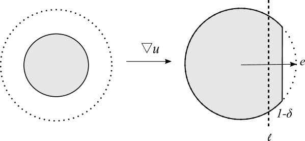
Figure 1: Improvement of oscillation for $\nabla u\cdot e$.

If the condition (4.1) is satisfied in all the directions $e\in\mathbb{S}^{n-1}$, then we obtain the improvement of oscillation for all $\nabla u\cdot e$, which lead to the improvement of oscillation for $|\nabla u|$. See Figure 2 and Corollary 4.2.

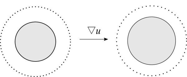
Figure 2: Improvement of oscillation for $|\nabla u|$.

Corollary 4.2.

Let $u$ be a smooth solution of (2.3) such that $|\nabla u|\leq 1$ in $Q_{1}$. For every $0<\ell<1$, $\mu>0$, there exist $\tau\in(0,1/4)$ depending only on $\mu$ and $n$, and $\delta>0$ depending only on $n,p,\mu,\ell$, such that for every nonnegative integer $k$, if

$$|\{(x,t)\in Q_{\tau^{i}}:\nabla u\cdot e\leq\ell(1-\delta)^{i}\}|>\mu|Q_{\tau^{i}}|\quad\mbox{for all }e\in\mathbb{S}^{n-1}\mbox{ and }i=0,\cdots,k,$$ (4.2)

then

$$|\nabla u|<(1-\delta)^{i+1}\quad\mbox{in }Q_{\tau^{i+1}}\ \mbox{ for all }i=0,\cdots,k.$$

Proof.

When $i=0$, it follows from Lemma 4.1 that $\nabla u\cdot e<1-\delta$ in $Q_{\tau}$ for all $e\in\mathbb{S}^{n-1}$. This implies that $|\nabla u|<1-\delta$ in $Q_{\tau}$.

Suppose this corollary holds for $i=0,\cdots,k-1$. We are going prove it for $i=k$. Let

$$v(x,t)=\frac{1}{\tau^{k}(1-\delta)^{k}}u(\tau^{k}x,\tau^{2k}t).$$

Then $v$ satisfies

$$v_{t}=\Delta v+(p-2)\frac{v_{i}v_{j}}{|\nabla v|^{2}+\varepsilon(1-\delta)^{-2k}}v_{ij}\quad\mbox{in }Q_{1}.$$

By the induction hypothesis, we also know that $|\nabla v|\leq 1$ in $Q_{1}$, and

$$|\{(x,t)\in Q_{1}:\nabla v\cdot e\leq\ell\}|>\mu|Q_{1}|\quad\mbox{for all }e\in\mathbb{S}^{n-1}.$$

Therefore, by Lemma 4.1 we have

$$\nabla v\cdot e\leq 1-\delta\quad\mbox{in }Q_{\tau}\quad\mbox{for all }e\in\mathbb{S}^{n-1}.$$

Hence, $|\nabla v|\leq 1-\delta$ in $Q_{\tau}$. Consequently,

$$|\nabla u|<(1-\delta)^{k+1}\quad\mbox{in }Q_{\tau^{k+1}}.$$

∎

4.2 Using the small oscillation

Unless $|\nabla u(0,0)|=0$, the condition in (4.2) will fail to be satisfied after finitely many steps of scaling in some direction $e\in\mathbb{S}^{n-1}$, in which we will then show that $u$ is close to some linear function so that Theorem 2.7 can be applied. See Lemma 4.4 and Figure 3.

Before that, we need a lemma which states that for a solution of a uniformly parabolic linear equation, if its oscillation in space is uniformly small in every time slice, then its oscillation in the space-time is also small.

Lemma 4.3.

Let $u\in C(\overline{Q}_{1})$ be a solution of (2.1) satisfying (2.2) and $A$ is a positive constant. Assume that for all $t\in[-1,0]$, we have

$$\mbox{ osc}_{B_{1}}u(\cdot,t)\leq A,$$

then

$$\mbox{ osc}_{Q_{1}}u\leq CA,$$

where $C$ is a positive constant depending only on $\Lambda$ and the dimension $n$.

Proof.

Let $\overline{w}(x,t)=\overline{a}+5n\Lambda At+2A|x|^{2}$, where $a$ is chosen so that $\overline{w}(\cdot,-1)\geq u(\cdot,-1)$ and $\overline{w}(\bar{x},-1)=u(\bar{x},-1)$ for some $\bar{x}\in\overline{B}_{1}$. If $\bar{x}\in\partial B_{1}$, then

$$2A=\overline{w}(\bar{x},-1)-\overline{w}(0,-1)\leq u(\bar{x},-1)-u(0,-1)\leq\mbox{ osc}_{B_{1}}u(\cdot-1)\leq A,$$

which is impossible. Therefore, $\bar{x}\in B_{1}$.

We claim that

$$\overline{w}\geq u\quad\text{in }Q_{1}.$$

If not, let $m=-\inf_{Q_{1}}(\overline{w}-u)>0$ and $(x_{0},t_{0})\in\overline{Q}_{1}$ be such that $m=u(x_{0},t_{0})-\overline{w}(x_{0},t_{0})$. By the choice of $\bar{a}$, we know that $t_{0}>-1$. Since $\overline{w}+m\geq u$ in $Q_{1}$, $\overline{w}(x_{0},t_{0})+m=u(x_{0},t_{0})$ and $\mbox{ osc}_{B_{1}}u(\cdot,t_{0})\leq A$, by the same reason in the above, we have $x_{0}\in B_{1}$. Therefore, we have that

$$(\overline{w}+m)_{t}-a_{ij}(x,t)\partial_{ij}(\overline{w}+m)\leq 0\quad\text{at }(x_{0},t_{0}).$$

This leads to

$$5n\Lambda A\leq 4A\cdot Tr(a_{ij})\leq 4n\Lambda A,$$

which is impossible. This proves the claim.

Similarly, one can show that for $\underline{w}(x,t)=\underline{a}-5n\Lambda At-2A|x|^{2}$, we have

$$\underline{w}\leq u\quad\text{in }Q_{1},$$

where $\underline{a}$ is chosen so that $\underline{w}(\cdot,-1)\leq u(\cdot,-1)$ and $\underline{w}(\underline{x},-1)=u(\underline{x},-1)$ for some $\underline{x}\in B_{1}$.

Meanwhile, since

$$\overline{w}(\bar{x},-1)-\underline{w}(\underline{x},-1)=u(\bar{x},-1)-u(\underline{x},-1)\leq osc_{B_{1}}u(\cdot,-1)\leq A,$$

we have

$$\bar{a}-\underline{a}\leq(10n\Lambda+1)A.$$

Therefore, we have

$$\mbox{ osc}_{Q_{1}}u\leq\sup_{Q_{1}}\overline{w}-\inf_{Q_{1}}\underline{w}\leq\bar{a}-\underline{a}+4A=(10n\Lambda+5)A.$$

∎

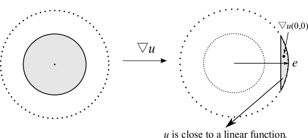
Figure 3: When $|\nabla u(0,0)|\neq 0$.

Lemma 4.4.

Let $\eta$ be a positive constant and $u$ be a smooth solution of (2.1) satisfying (2.2). Assume $|\nabla u|\leq 1$ everywhere and

$$\left|\left\{(x,t)\in Q_{1}:|\nabla u-e|>\varepsilon_{0}\right\}\right|\leq\varepsilon_{1}$$

for some $e\in\mathbb{S}^{n-1}$ and two positive constants $\varepsilon_{0},\varepsilon_{1}.$ Then, if $\varepsilon_{0}$ and $\varepsilon_{1}$ are sufficiently small, there exists a constant $a\in\mathbb{R}$, such that

$$|u(x,t)-a-e\cdot x|\leq\eta\quad\text{ for all }(x,t)\in Q_{1/2}.$$

Here, both $\varepsilon_{0}$ and $\varepsilon_{2}$ depend only on $n,\lambda,\Lambda$ and $\eta$.

Proof.

Let $f(t):=|\{x\in B_{1}:|\nabla u(x,t)-e|>\varepsilon_{0}\}|$. By the assumptions and Fubini’s theorem, we have that $\int_{-1}^{0}f(t)\mathrm{d}t\leq\varepsilon_{1}$. It follows that for $E:=\{t\in(-1,0):f(t)\geq\sqrt{\varepsilon_{1}}\}$, we obtain

$$|E|\leq\frac{1}{\sqrt{\varepsilon_{1}}}\int_{E}f(t)\mathrm{d}t\leq\frac{1}{\sqrt{\varepsilon_{1}}}\int_{-1}^{0}f(t)\mathrm{d}t\leq\sqrt{\varepsilon_{1}}.$$

Therefore, for all $t\in(-1,0]\setminus E$, with $|E|\leq\sqrt{\varepsilon_{1}}$, we have

$$|\{x\in B_{1}:|\nabla u(x,t)-e|>\varepsilon_{0}\}|\leq\sqrt{\varepsilon_{1}}.$$ (4.3)

It follows from (4.3) and Morrey’s inequality (see, e.g., Section 5.6.2 in the book [13]) that for all $t\in(-1,0]\setminus E$, we have

$$\mbox{ osc}_{B_{1/2}}(u(\cdot,t)-e\cdot x)\leq C(n)\|\nabla u-e\|_{L^{2n}(B_{1})}\leq C(n)(\varepsilon_{0}+\varepsilon_{1}^{\frac{1}{4n}}),$$ (4.4)

where $C(n)>0$ depends only on $n$.

Meanwhile, since $|\nabla u|\leq 1$ in $Q_{1}$, we have that $\mbox{ osc}_{B_{1}}u(\cdot,t)\leq 2$ for all $t\in(-1,0]$. Thus, applying Lemma 4.3, we have that $\mbox{ osc}_{Q_{1}}u\leq C$ for some constant $C$. The function $u$ is a solution of a uniformly parabolic equation. By Theorem 2.4, we have

$$\|u\|_{C^{\alpha}(Q_{1/2})}\leq C$$

for some positive constants $\alpha$ and $C$ depending only on $\lambda,\Lambda,n$. Therefore, by (4.4) and the fact that $|E|\leq\sqrt{\varepsilon_{1}}$, we obtain

$$\mbox{ osc}_{B_{1/2}}(u(\cdot,t)-e\cdot x)\leq C(\varepsilon_{0}+\varepsilon_{1}^{\frac{1}{4n}}+\varepsilon_{1}^{\frac{\alpha}{4}})$$

for all $t\in(-1/4,0]$ (that is, including $t\in E$). By Lemma 4.3, we obtain

$$\mbox{ osc}_{Q_{1/2}}(u-e\cdot x)\leq C(\varepsilon_{0}+\varepsilon_{1}^{\frac{1}{4n}}+\varepsilon_{1}^{\frac{\alpha}{4}}),$$

where $C>0$ depends only on $\lambda,\Lambda,n$. Hence, if $\varepsilon_{0}$ and $\varepsilon_{1}$ are sufficiently small, there exists a constant $a\in\mathbb{R}$, such that

$$|u(t,x)-a-e\cdot x|\leq\eta\quad\text{ for all }(x,t)\in Q_{1/2}.$$

∎

4.3 Iteration

In this section, we finish our proof of the following a priori estimates.

Theorem 4.5.

Let $u$ be a smooth solution of (2.3) in $Q_{1}$. Then there exist two positive constants $\alpha$ and $C$ depending only on $n$ and $p$ such that

$$\|\nabla u\|_{C^{\alpha}(Q_{1/2})}\leq C(\|u\|_{L^{\infty}(Q_{1})}+\varepsilon).$$

Also, there holds

$$\sup_{(x,t),(x,s)\in Q_{1/2}}\frac{|u(x,t)-u(x,s)|}{|t-s|^{\frac{1+\alpha}{2}}}\leq C(\|u\|_{L^{\infty}(Q_{1})}+\varepsilon).$$

Proof.

We first show the Hölder estimate of $\nabla u$ at $(0,0)$. Moreover, by normalization, we may assume that $u(0,0)=0$ and $|\nabla u|\leq 1$ in $Q_{1}$.

Let $\eta$ be the one in Theorem 2.7 with $\gamma=1/2$, and for this $\eta$, let $\varepsilon_{0},\varepsilon_{1}$ be two sufficiently small positive constants so that the conclusion of Lemma 4.4 holds. For $\ell=1-\varepsilon_{0}^{2}/2$ and $\mu=\varepsilon_{1}/|Q_{1}|$, if

$$|\{(x,t)\in Q_{1}:\nabla u\cdot e\leq\ell\}|\leq\mu|Q_{1}|\quad\mbox{for any }e\in\mathbb{S}^{n-1},$$

then

$$\left|\left\{(x,t)\in Q_{1}:|\nabla u-e|>\varepsilon_{0}\right\}\right|\leq\varepsilon_{1}.$$

This is because if $|\nabla u(x,t)-e|>\varepsilon_{0}$ for some $(x,t)\in Q_{1}$, then

$$|\nabla u|^{2}-2\nabla u\cdot e+1\geq\varepsilon_{0}^{2}.$$

Since $|\nabla u|\leq 1$, we have

$$\nabla u\cdot e\leq 1-\varepsilon_{0}^{2}/2.$$

Therefore, if $\ell=1-\varepsilon_{0}^{2}/2$ and $\mu=\varepsilon_{1}/|Q_{1}|$, then

$$\left\{(x,t)\in Q_{1}:|\nabla u-e|>\varepsilon_{0}\right\}\subset\{(x,t)\in Q_{1}:\nabla u\cdot e\leq\ell\},$$

from which it follows that

$$\left|\left\{(x,t)\in Q_{1}:|\nabla u-e|>\varepsilon_{0}\right\}\right|\leq\left|\{(x,t)\in Q_{1}:\nabla u\cdot e\leq\ell\}\right|\leq\mu|Q_{1}|\leq\varepsilon_{1}.$$

Let $\tau,\delta$ be the constants in Corollary 4.2. Let $k$ be the minimum nonnegative integer such that the condition (4.2) does not hold. If $k=\infty$, then it follows immediately from Corollary 4.2 that

$$|\nabla u(x,t)|\leq C(|x|+\sqrt{|t|})^{\alpha}\quad\mbox{for all }(x,t)\in Q_{1},$$

where $C=(1-\delta)^{-1}$ and $\alpha=\log(1-\delta)/\log\tau$.

If $k$ is finite, then

$$|\{(x,t)\in Q_{\tau^{k}}:\nabla u\cdot e\leq\ell(1-\delta)^{k}\}|\leq\mu|Q_{\tau^{k}}|\quad\mbox{for some }e\in\mathbb{S}^{n-1}.$$

Let

$$v(x,t)=\frac{1}{\tau^{k}(1-\delta)^{k}}u(\tau^{k}x,\tau^{2k}t).$$

Then $v$ satisfies

$$v_{t}=\Delta v+(p-2)\frac{v_{i}v_{j}}{|\nabla v|^{2}+\varepsilon(1-\delta)^{-2k}}v_{ij}\quad\mbox{in }Q_{1},$$

and

$$|\{(x,t)\in Q_{1}:\nabla v\cdot e\leq\ell\}|\leq\mu|Q_{1}|\quad\mbox{for some }e\in\mathbb{S}^{n-1}.$$

Consequently,

$$\left|\left\{(x,t)\in Q_{1}:|\nabla v-e|>\varepsilon_{0}\right\}\right|\leq\varepsilon_{1}.$$

Since condition (4.2) holds for $k-1$, then $|\nabla v|\leq 1$ in $Q_{1}$. It follows from Lemma 4.4 that there exists $a\in\mathbb{R}$ such that

$$|v(x,t)-a-e\cdot x|\leq\eta\quad\text{ for all }(x,t)\in Q_{1/2}.$$

By Theorem 2.7 that there exists $b\in\mathbb{R}^{n}$ such that

$$|\nabla v-b|\leq C(|x|+\sqrt{|t|})\quad\mbox{for all }(x,t)\in Q_{1/4}.$$

Since $|\nabla v|\leq 1$ and $|b|\leq 1$, there also holds

$$|\nabla v-b|\leq C(|x|+\sqrt{|t|})\quad\mbox{for all }(x,t)\in Q_{1}.$$

Rescaling back, we obtain

$$|\nabla u-(1-\delta)^{k}b|\leq C(1-\delta)^{k}\tau^{-k}(|x|+\sqrt{|t|})\leq C(|x|+\sqrt{|t|})^{\alpha}\quad\mbox{for all }(x,t)\in Q_{\tau^{k}}.$$

On the other hand, we know that

$$|\nabla u|<(1-\delta)^{i}\quad\mbox{in }Q_{\tau^{i}}\mbox{ and for all }i=0,\cdots,k.$$

This implies that

$$|\nabla u-(1-\delta)^{k}b|\leq C(|x|+\sqrt{|t|})^{\alpha}\quad\mbox{for all }(x,t)\in Q_{1}\setminus Q_{\tau^{k}}.$$

Therefore,

$$|\nabla u-(1-\delta)^{k}b|\leq C(|x|+\sqrt{|t|})^{\alpha}\quad\mbox{for all }(x,t)\in Q_{1}.$$

In conclusion, we have proved that there exist $q\in\mathbb{R}^{n}$ with $|q|\leq 1$, and two positive constants $\alpha,C$ such that

$$|\nabla u(x,t)-q|\leq C(|x|+\sqrt{|t|})^{\alpha}\quad\mbox{for all }(x,t)\in Q_{1}.$$

By standard translation arguments, it follows that

$$\|\nabla u\|_{C^{\alpha}(Q_{1/2})}\leq C(\|u\|_{L^{\infty}(Q_{1})}+\varepsilon).$$ (4.5)

Now, we are going to prove the $C^{\frac{1+\alpha}{2}}$ continuity of $u$ in the time variable $t$.

Let $t\in[-1/4,0)$ and $r=\sqrt{|t|}$. For $(y,s)\in Q_{r}$, let

$$w(y,s)=u(y,s)-u(0,0)-\nabla u(0,0)\cdot y.$$

By (4.5), we have

$$|u(y,s)-u(0,s)-\nabla u(0,s)\cdot y|\leq C(\|u\|_{L^{\infty}(Q_{1})}+\varepsilon)|y|^{1+\alpha},$$ (4.6)

Therefore, for $y_{1},y_{2}\in B_{r}$,

$$|w(y_{1},s)-w(y_{2},s)|$$

$$=|u(y_{1},s)-u(y_{2},s)-\nabla u(0,0)\cdot(y_{1}-y_{2})|$$

$$\leq|(\nabla u(0,s)-\nabla u(0,0))\cdot(y_{1}-y_{2})|+C(\|u\|_{L^{\infty}(Q_{1})}+\varepsilon)r^{1+\alpha}$$

$$\leq C(\|u\|_{L^{\infty}(Q_{1})}+\varepsilon)|s|^{\frac{\alpha}{2}}|y_{1}-y_{2}|+C(\|u\|_{L^{\infty}(Q_{1})}+\varepsilon)r^{1+\alpha}$$

$$\leq C(\|u\|_{L^{\infty}(Q_{1})}+\varepsilon)r^{1+\alpha},$$

where in the first inequality we used (4.6) and in the second inequality we used (4.5). Since $u$ satisfies (2.3), $w$ satisfies a uniformly parabolic equation as well. By Lemma 4.3, we have

$$\mbox{ osc}_{Q_{r}}w\leq C(\|u\|_{L^{\infty}(Q_{1})}+\varepsilon)r^{1+\alpha}.$$

In particular,

$$|u(0,t)-u(0,0)|\leq C(\|u\|_{L^{\infty}(Q_{1})}+\varepsilon)|t|^{\frac{1+\alpha}{2}}.$$

By standard translation arguments, it follows that

$$\sup_{(x,t),(x,s)\in Q_{1/2}}\frac{|u(x,t)-u(x,s)|}{|t-s|^{\frac{1+\alpha}{2}}}\leq C(\|u\|_{L^{\infty}(Q_{1})}+\varepsilon).$$

This finishes the proof of this theorem. ∎

5 Approximations and the proof of our main result

This section is devoted to the final step of our proof of Theorem 1.1, that is the approximation step.

Note that (2.3) is a uniformly parabolic quasilinear equation and its coefficients $a_{ij}(q)$ as in (2.4) are smooth with bounded derivatives (for each value of $\varepsilon>0$). The next lemma follows directly from classical quasilinear equations theory (see, e.g., Theorem 4.4 of [32] in page 560) and the Schauder estimates.

Lemma 5.1.

Let $g\in C(\partial_{p}Q_{1})$. For $\varepsilon>0$, there exists a unique solution $u^{\varepsilon}\in C^{\infty}(Q_{1})\cap C(\overline{Q}_{1})$ of (2.3) such that $u^{\varepsilon}=g$ on $\partial_{p}Q_{1}$.

We are now ready to prove Theorem 1.1 by taking $\varepsilon\to 0$ in the a priori estimate of Theorem 4.5.

Proof of Theorem 1.1.

Without loss of generality, we assume that $u\in C(\overline{Q}_{1})$. Let $\omega$ be its modulus of continuity in $\overline{Q}_{1}$. By Lemma 5.1, for $\varepsilon\in(0,1)$, there exists a unique solution $v^{\varepsilon}\in C^{\infty}(Q_{1})\cap C(\overline{Q}_{1})$ of (2.3) such that $v^{\varepsilon}=u$ on $\partial_{p}Q_{1}$. Moreover, it follows from Theorem 2.5 that there exists a modulus of continuity $\omega^{*}$, which depends only on $n,p,\omega,\|u\|_{L^{\infty}(\partial_{p}Q_{1})}$, such that

$$|v^{\varepsilon}(x,t)-v^{\varepsilon}(y,s)|\leq\omega^{*}(|x-y|\vee\sqrt{|s-t|})\quad\mbox{ for all }(x,t),(y,s)\in\overline{Q}_{1}.$$

By the maximum principle,

$$\|v^{\varepsilon}\|_{L^{\infty}(Q_{1})}\leq\|u\|_{L^{\infty}(\partial_{p}Q_{1})}.$$

It follows from Ascoli-Arzela theorem that there exists a subsequence $\{v^{\varepsilon_{k}}\}$ such that $v^{\varepsilon_{k}}\to v\in C(\overline{Q}_{1})$ uniformly in $\overline{Q}_{1}$ as $\varepsilon_{k}\to 0$. By the stability property in Theorem 2.10, $v$ is a viscosity solution of (1.5). By the comparison principle in Theorem 2.9, we obtain that $u\equiv v$ in $\overline{Q}_{1}$.

On the other hand, it follows from Theorem 4.5 that, subject to a subsequence, $\nabla v^{\varepsilon_{k}}$ converges in $C^{\alpha}(Q_{1/2})$ for some constant $\alpha$ depending only on $n$ and $p$. Therefore, $u$ is differentiable in $x$ everywhere in $Q_{1/2}$, and thus, $\nabla v^{\varepsilon_{k}}$ converges to $\nabla u$ in $C^{\alpha}(Q_{1/2})$. Since

$$\|\nabla v^{\varepsilon_{k}}\|_{C^{\alpha}(Q_{1/2})}\leq C(\|v^{\varepsilon_{k}}\|_{L^{\infty}(Q_{1})}+\varepsilon_{k})\leq C(\|u\|_{L^{\infty}(Q_{1})}+\varepsilon_{k}),$$

where $C>0$ depends only on $n$ and $p$, we obtain

$$\|\nabla u\|_{C^{\alpha}(Q_{1/2})}\leq C\|u\|_{L^{\infty}(Q_{1})}$$

by sending $k\to\infty$.

We also know from Theorem 4.5 that for all $(x,t),(x,s)\in Q_{1/2}$, there holds

$$|v^{\varepsilon_{k}}(x,t)-v^{\varepsilon_{k}}(x,s)|\leq C(\|u\|_{L^{\infty}(Q_{1})}+\varepsilon_{k})|t-s|^{\frac{1+\alpha}{2}}.$$

By sending $k\to\infty$, we obtain

$$\sup_{(x,t),(x,s)\in Q_{1/2}}\frac{|u(x,t)-u(x,s)|}{|t-s|^{\frac{1+\alpha}{2}}}\leq C\|u\|_{L^{\infty}(Q_{1})}.$$

This finishes the proof of Theorem 1.1. ∎

Appendix A Appendix A

In this section we provide a proof of Lemma 3.1

Proof of Lemma 3.1..

In the following, we denote $V=|\nabla u|^{2}+\varepsilon^{2}$. First,

$$\partial_{t}\varphi =pV^{\frac{p-2}{2}}\nabla u\cdot\nabla u_{t}$$

$$=pV^{\frac{p-2}{2}}u_{k}\Big{(}\Delta u_{k}-2(p-2)V^{-2}u_{l}u_{kl}u_{i}u_{j}u_{ij}+2(p-2)V^{-1}u_{ik}u_{ij}u_{j}$$

$$\quad\quad+(p-2)V^{-1}u_{i}u_{j}u_{ijk}\Big{)}$$

$$=pV^{\frac{p-2}{2}}\Big{(}u_{k}\Delta u_{k}-2(p-2)V^{-2}(\Delta_{\infty}u)^{2}+2(p-2)V^{-1}|\nabla^{2}u\nabla u|^{2}$$

$$\quad\quad+(p-2)V^{-1}u_{i}u_{j}u_{k}u_{ijk}\Big{)},$$

where $\Delta_{\infty}u=\sum_{i,j}u_{ij}u_{i}u_{j}$. Secondly,

$$\partial_{j}\varphi=pV^{\frac{p-2}{2}}u_{k}u_{kj},$$

and therefore,

$$\partial_{ij}\varphi =p(p-2)V^{\frac{p-4}{2}}u_{l}u_{li}u_{k}u_{kj}+pV^{\frac{p-2}{2}}u_{ki}u_{kj}+pV^{\frac{p-2}{2}}u_{k}u_{kij}.$$

Consequently,

$$a_{ij}(\nabla u)\partial_{ij}\varphi =p(p-2)V^{\frac{p-4}{2}}u_{l}u_{li}u_{k}u_{ki}+pV^{\frac{p-2}{2}}u_{ki}u_{ki}+pV^{\frac{p-2}{2}}u_{k}u_{kii}$$

$$\quad+p(p-2)^{2}V^{\frac{p-6}{2}}u_{i}u_{j}u_{l}u_{li}u_{k}u_{kj}$$

$$\quad+p(p-2)V^{\frac{p-4}{2}}u_{ki}u_{kj}u_{i}u_{j}$$

$$\quad+p(p-2)V^{\frac{p-4}{2}}u_{i}u_{j}u_{k}u_{ijk}$$

$$=2p(p-2)V^{\frac{p-4}{2}}|\nabla^{2}u\nabla u|^{2}+pV^{\frac{p-2}{2}}|\nabla^{2}u|^{2}+pV^{\frac{p-2}{2}}u_{k}\Delta u_{k}$$

$$\quad+p(p-2)^{2}V^{\frac{p-6}{2}}(\Delta_{\infty}u)^{2}$$

$$\quad+p(p-2)V^{\frac{p-4}{2}}u_{i}u_{j}u_{k}u_{ijk}.$$

Therefore,

$$\big{(}\partial_{t}-a_{ij}(\nabla u)\partial_{ij}\big{)}\varphi=pV^{\frac{p-6}{2}}\Big{(}p(2-p)(\Delta_{\infty}u)^{2}-|\nabla^{2}u|^{2}V^{2}\Big{)}\leq 0,$$

where in the last inequality we used the Hölder inequality that

$$(\Delta_{\infty}u)^{2} =\left(\sum_{i,j}u_{ij}u_{i}u_{j}\right)^{2}$$

$$\leq\left(\sum_{i,j}u_{ij}^{2}\right)\left(\sum_{i,j}u_{i}^{2}u_{j}^{2}\right)=|\nabla^{2}u|^{2}|\nabla u|^{4}\leq|\nabla^{2}u|^{2}V^{2}.$$

∎

Appendix B Appendix B

In this second appendix, we shall prove the boundary estimates in Proposition 2.5. Recall that for two real numbers $a$ and $b$, we denote $a\vee b=\max(a,b)$, $a\wedge b=\min(a,b)$.

Lemma B.1.

There exists a non negative continuous function $\psi:\mathbb{R}^{n}\times(-\infty,0]\to\mathbb{R}$ such that

• $\psi=0\quad\mbox{in }B_{1}\times\{t=0\}$;

• $\psi_{t}-a_{ij}(x,t)\psi_{ij}\geq 0\quad\mbox{in }(\mathbb{R}^{n}\setminus B_{1})\times(-\infty,0]$;

• $\psi\geq 1\quad\mbox{in }(\mathbb{R}^{n}\times(-\infty,0])\setminus(B_{2}\times[-1,0])$,

where $a_{ij}(x,t)$ satisfies (2.2).

Proof.

Let $v(x)=\sqrt{(|x|-1)^{+}}$. It follows from elementary calculations that there exists $\delta\in(0,1)$ such that

$$-a_{ij}v_{ij}\geq 1\quad\mbox{for }1<|x|<1+\delta.$$

Then $\psi=\min(\delta^{-1/2}v(x)-t,1)$ is a desired function. ∎

Lemma B.2.

Let $u\in C(\overline{Q}_{1})$ be a solution of (2.1) satisfying (2.2). Let $(x,t)\in\partial B_{1}\times(-1,0]$ be fixed, $\rho$ be a modulus of continuity such that

$$|u(y,s)-u(x,t)|\leq\rho(|x-y|\vee\sqrt{|t-s|})$$

for all $(y,s)\in\partial_{p}(B_{1}\times(-1,t])$. Then there exists another modulus of continuity $\rho^{*}$ depending only on $n,\lambda,\Lambda,\rho,\|u\|_{L^{\infty}(\partial_{p}Q_{1})}$ such that

$$|u(x,t)-u(y,s)|\leq\rho^{*}(|x-y|\vee\sqrt{|t-s|})$$

for all $(y,s)\in\overline{B}_{1}\times[-1,t]$.

Proof.

Fix $r\in(0,1)$. Let $x_{r}=(1+r)x$ and $\psi$ be as in Lemma B.1. Define

$$v(y,s)=u(x,t)+\rho(3r)+2\|u\|_{L^{\infty}(\partial_{p}Q_{1})}\psi\left(\frac{y-x_{r}}{r},\frac{s-t}{r^{2}}\right).$$

Then

$$v_{s}-a_{ij}v_{ij}\geq 0\quad\mbox{in }\Omega:=(B_{3r}(x)\cap B_{1})\times(-1,t].$$

For $(y,s)\in\partial_{p}\Omega$ and $|y-x|\vee\sqrt{|s-t|}<3r$, then

$$v(y,s)\geq u(x,t)+\rho(3r)\geq u(y,s).$$

For $(y,s)\in\partial_{p}\Omega$ and $|y-x|\vee\sqrt{|s-t|}\geq 3r$, then

$$v(y,s)\geq u(x,t)+2\|u\|_{L^{\infty}(\partial_{p}Q_{1})}=u(x,t)+2\|u\|_{L^{\infty}(Q_{1})}\geq u(y,s).$$

It follows from the maximum principle that $v\geq u$ in $\Omega$, i.e.,

$$\rho(3r)+2\|u\|_{L^{\infty}(\partial_{p}Q_{1})}\psi\left(\frac{y-x_{r}}{r},\frac{s-t}{r^{2}}\right)\geq u(y,s)-u(x,t).$$

Similarly, one can show that

$$\rho(3r)+2\|u\|_{L^{\infty}(\partial_{p}Q_{1})}\psi\left(\frac{y-x_{r}}{r},\frac{s-t}{r^{2}}\right)\geq u(x,t)-u(y,s).$$

Therefore, for $(y,s)\in\overline{\Omega}$.

$$|u(x,t)-u(y,s)|\leq\rho(3r)+2\|u\|_{L^{\infty}(\partial_{p}Q_{1})}\psi\left(\frac{y-x_{r}}{r},\frac{s-t}{r^{2}}\right).$$ (B.1)

It is clear from the definition of $\psi$ that (B.1) holds for $(y,s)\in(B_{1}\setminus B_{3r}(x))\times(-1,t]$ as well. Meanwhile

$$\psi\left(\frac{y-x_{r}}{r},\frac{s-t}{r^{2}}\right)=\psi\left(\frac{y-x_{r}}{r},\frac{s-t}{r^{2}}\right)-\psi\left(\frac{x-x_{r}}{r},0\right)\leq\overline{\rho}((|x-y|\vee\sqrt{|t-s|})/r),$$

where $\overline{\rho}$ is a modulus continuity of $\psi$. Therefore, we have for $(y,s)\in\overline{B}_{1}\times[-1,t]$,

$$|u(x,t)-u(y,s)|\leq\rho(3r)+2\|u\|_{L^{\infty}(\partial_{p}Q_{1})}\overline{\rho}((|x-y|\vee\sqrt{|t-s|})/r).$$

The conclusion then follows from the observation that

$$\rho^{*}(d)=\inf_{r\in(0,1)}\left(\rho(3r)+2\|u\|_{L^{\infty}(\partial_{p}Q_{1})}\overline{\rho}(d/r)\right)$$

is a modulus of continuity. ∎

Lemma B.3.

Let $t\in[-1,0)$ and $u\in C(\overline{B}_{1}\times[t,0])$ be a solution of (2.1) in $B_{1}\times(t,0]$ satisfying (2.2). Let $x\in\overline{B}_{1}$ be fixed, $\rho$ be a modulus of continuity such that

$$|u(y,s)-u(x,t)|\leq\rho(|x-y|\vee\sqrt{|s-t|})$$

for all $(y,s)\in\partial_{p}(B_{1}\times(t,0])$. Then there exists another modulus of continuity $\rho^{*}$ depending only on $n,\lambda,\Lambda,\rho$ and $\|u\|_{L^{\infty}(\partial_{p}(B_{1}\times(t,0]))}$ such that

$$|u(x,t)-u(y,s)|\leq\rho^{*}(|x-y|\vee\sqrt{|s-t|})$$

for all $(y,s)\in\overline{B}_{1}\times[t,0]$.

Proof.

Let $b\in C^{\infty}(\mathbb{R}^{n})$ be a nonnegative function such that $b\equiv 1$ in $\mathbb{R}^{n}\setminus B_{1}$ and $b(0)=0$. Let

$$\phi(y,s)=b(y)+Ms,$$

where $M=\sup_{B_{1}\times(t,0]}|a_{ij}|\sup_{\mathbb{R}^{n}}|\nabla^{2}b|+1$, and $\overline{\rho}$ be its modulus of continuity. Define

$$v(y,s)=u(x,t)+\rho(r)+2\|u\|_{L^{\infty}(\partial_{p}(B_{1}\times(t,0]))}\phi\Big{(}\frac{y-x}{r},\frac{s-t}{r^{2}}\Big{)}.$$

Then

$$v_{s}-a_{ij}v_{ij}\geq 0\quad\mbox{in }B_{1}\times(t,0].$$

For $(y,s)\in\partial_{p}(B_{1}\times(t,0])$ and $|y-x|\vee\sqrt{|s-t|}<r$, then

$$v(y,s)\geq u(x,t)+\rho(r)\geq u(y,s).$$

For $(y,s)\in\partial_{p}(B_{1}\times(t,0])$ and $|y-x|\vee\sqrt{|s-t|}\geq r$, then either $|y-x|\geq r$ or $|s-t|\geq r^{2}$, each of which implies that

$$v(y,s)\geq u(x,t)+2\|u\|_{L^{\infty}(\partial_{p}(B_{1}\times(t,0]))}=u(x,t)+2\|u\|_{L^{\infty}(B_{1}\times(t,0])}\geq u(y,s).$$

It follows from the maximum principle that $v\geq u$ in $\overline{Q}_{1}$, i.e.,

$$\rho(r)+2\|u\|_{L^{\infty}(\partial_{p}(B_{1}\times(t,0]))}\phi\Big{(}\frac{y-x}{r},\frac{s-t}{r^{2}}\Big{)}\geq u(y,s)-u(x,t).$$

Similarly, one can show that

$$\rho(r)+2\|u\|_{L^{\infty}(\partial_{p}(B_{1}\times(t,0]))}\phi\Big{(}\frac{y-x}{r},\frac{s-t}{r^{2}}\Big{)}\geq u(x,t)-u(y,s).$$

Meanwhile

$$\phi\left(\frac{y-x}{r},\frac{s-t}{r^{2}}\right)=\phi\left(\frac{y-x}{r},\frac{s-t}{r^{2}}\right)-\phi(0,0)\leq\overline{\rho}((|x-y|\vee\sqrt{|s-t|})/r),$$

where $\overline{\rho}$ is a modulus continuity of $\phi$. Therefore, we have

$$|u(x,t)-u(y,s)|\leq\rho(r)+2\|u\|_{L^{\infty}(\partial_{p}(B_{1}\times(t,0]))}\overline{\rho}((|x-y|\vee\sqrt{|s-t|})/r).$$

The conclusion then follows from the observation that

$$\rho^{*}(d)=\inf_{r\in(0,1)}\left(\rho(r)+2\|u\|_{L^{\infty}(\partial_{p}(B_{1}\times(t,0]))}\overline{\rho}(d/r)\right)$$

is a modulus of continuity. ∎

Lemma B.4.

Let $u\in C(\overline{Q}_{1})$ be a solution of (2.1) satisfying (2.2). Let $(x,t)\in\partial B_{1}\times(-1,0]$ be fixed, $\rho$ be a modulus of continuity such that

$$|u(y,s)-u(x,t)|\leq\rho(|x-y|\vee\sqrt{|t-s|})$$

for all $(y,s)\in\partial_{p}Q_{1}$. Then there exists another modulus of continuity $\rho^{*}$ depending only on $n,\lambda,\Lambda,\rho,\|u\|_{L^{\infty}(\partial_{p}Q_{1})}$ such that

$$|u(x,t)-u(y,s)|\leq\rho^{*}(|x-y|\vee\sqrt{|t-s|})$$

for all $(y,s)\in\overline{Q}_{1}$.

Proof.

It follows from Lemma B.2 that there exists a modulus of continuity $\rho_{1}$ depending only on $n,\lambda,\Lambda,\rho,\|u\|_{L^{\infty}(\partial_{p}Q_{1})}$ such that

$$|u(x,t)-u(y,s)|\leq\rho_{1}(|x-y|\vee\sqrt{|t-s|})$$

for all $(y,s)\in\overline{B}_{1}\times[-1,t]$. If $t<0$, by applying Lemma B.3 to the cylinder $B_{1}\times(t,0)$ and noticing that $\|u\|_{L^{\infty}(\partial_{p}(B_{1}\times(t,0]))}\leq\|u\|_{L^{\infty}(Q_{1})}\leq\|u\|_{L^{\infty}(\partial_{p}Q_{1})}$, we conclude that there exists a modulus of continuity $\rho_{2}$ depending only on $n,\lambda,\Lambda,\rho,\|u\|_{L^{\infty}(\partial_{p}Q_{1})}$ such that

$$|u(x,t)-u(y,s)|\leq\rho_{2}(|x-y|\vee\sqrt{|t-s|})$$

for all $(y,s)\in\overline{B}_{1}\times[t,0]$. Finally, the choice of $\rho^{*}=\rho_{1}+\rho_{2}$ is the desired one. ∎

Corollary B.5.

Let $u\in C(\overline{Q}_{1})$ be a solution of (2.1) satisfying (2.2). Let $(x,t)\in\partial_{p}Q_{1}$ be fixed, $\rho$ be a modulus of continuity such that

$$|u(y,s)-u(x,t)|\leq\rho(|x-y|\vee\sqrt{|t-s|})$$

for all $(y,s)\in\partial_{p}Q_{1}$. Then there exists another modulus of continuity $\tilde{\rho}$ depending only on $n,\lambda,\Lambda,\rho,\|u\|_{L^{\infty}(\partial_{p}Q_{1})}$ such that

$$|u(x,t)-u(y,s)|\leq\tilde{\rho}(|x-y|\vee\sqrt{|t-s|})$$

for all $(y,s)\in\overline{Q}_{1}$.

Proof.

It follows from Lemma B.3 and Lemma B.4. ∎

Proof of Proposition 2.5.

Let $(x,t),(y,s)\in Q_{1}$, and we assume that $t\geq s$. Let

$$d_{X}=\min(1-|x|,\sqrt{t+1}),$$

and $x_{0}$ be such that $|x-x_{0}|=1-|x|$. Let $\tilde{\rho}$ be the one in the conclusion of Corollary B.5.

Case 1: $(1-|x|)^{2}\leq(1+t)$. Then $d_{X}=1-|x|$.

If $(y,s)\in B_{d_{X}/2}(x)\times(t-d_{X}^{2}/4,t]$, then by the interior Hölder estimates Theorem 2.4, we have

$$d_{X}^{\alpha}\frac{|u(x,t)-u(y,s)|}{(|x-y|\vee\sqrt{t-s})^{\alpha}}\leq C\|u-u(x_{0},t)\|_{L^{\infty}(B_{d_{X}}(x)\times(t-d_{X}^{2},t])}\leq C\tilde{\rho}(2d_{X}).$$

Suppose that $2^{-m-1}d_{X}\leq|x-y|\vee\sqrt{t-s}\leq 2^{-m}d_{X}$ for some integer $m\geq 1$. Then

$$|u(x,t)-u(y,s)|\leq C\frac{\tilde{\rho}(2^{m+2}(|x-y|\vee\sqrt{t-s}))}{2^{m\alpha}}.$$

Notice that

$$\rho_{1}(d):=C\sup_{m\geq 1}\frac{\tilde{\rho}(2^{m+2}d)}{2^{m\alpha}}$$

is a modulus of continuity, and therefore,

$$|u(x,t)-u(y,s)|\leq\rho_{1}(|x-y|\vee\sqrt{t-s}).$$

If $(y,s)\not\in B_{d_{X}/2}(x)\times(t-d_{X}^{2}/4,t]$, then

$$\begin{split}|u(x,t)-u(y,s)|&\leq|u(x,t)-u(x_{0},t)|+|u(x_{0},t)-u(y,s)|\\ &\leq\tilde{\rho}(d_{X})+\tilde{\rho}(|x_{0}-y|\vee\sqrt{|t-s|})\\ &\leq\tilde{\rho}(2(|x-y|\vee\sqrt{|t-s|}))+\tilde{\rho}((|x-y|+d_{X})\vee\sqrt{|t-s|})\\ &\leq\tilde{\rho}(2(|x-y|\vee\sqrt{|t-s|}))+\tilde{\rho}(3(|x-y|\vee\sqrt{|t-s|}))\\ &\leq 2\tilde{\rho}(3(|x-y|\vee\sqrt{|t-s|})).\end{split}$$

Case 2: $(1-|x|)^{2}\geq(1+t)$. Then $d_{X}=t+1$.

As before, if $(y,s)\in B_{d_{X}/2}(x)\times(t-d_{X}^{2}/4,t]$, then we have

$$d_{X}^{\alpha}\frac{|u(x,t)-u(y,s)|}{(|x-y|\vee\sqrt{t-s})^{\alpha}}\leq C\|u-u(x,-1)\|_{L^{\infty}(B_{d_{X}}(x)\times(t-d_{X}^{2},t])}\leq C\tilde{\rho}(2d_{X}),$$

and therefore,

$$|u(x,t)-u(y,s)|\leq\rho_{1}(|x-y|\vee\sqrt{t-s}).$$

If $(y,s)\not\in B_{d_{X}/2}(x)\times(t-d_{X}^{2}/4,t]$, then

$$\begin{split}|u(x,t)-u(y,s)|&\leq|u(x,t)-u(x,-1)|+|u(x,-1)-u(y,s)|\\ &\leq\tilde{\rho}(d_{X})+\tilde{\rho}(|x-y|\vee\sqrt{|1+s|})\\ &\leq\tilde{\rho}(2(|x-y|\vee\sqrt{|t-s|}))+\tilde{\rho}(|x-y|\vee\sqrt{|1+t|})\\ &\leq\tilde{\rho}(2(|x-y|\vee\sqrt{|t-s|}))+\tilde{\rho}(3(|x-y|\vee\sqrt{|t-s|}))\\ &\leq 2\tilde{\rho}(3(|x-y|\vee\sqrt{|t-s|})).\end{split}$$

∎

T. Jin

Department of Mathematics, The Hong Kong University of Science and Technology
Clear Water Bay, Kowloon, Hong Kong

and

Department of Computing and Mathematical Sciences, California Institute of Technology
1200 E. California Blvd., MS 305-16, Pasadena, CA 91125, USA
Email: tianlingjin@ust.hk / tianling@caltech.edu

L. Silvestre

Department of Mathematics, The University of Chicago
5734 S. University Avenue, Chicago, IL 60637, USA
Email: luis@math.uchicago.edu

References

- [1] A. Banerjee and N. Garofalo. Gradient bounds and monotonicity of the energy for some nonlinear singular diffusion equations. Indiana Univ. Math. J., 62(2):699–736, 2013.
- [2] A. Banerjee and N. Garofalo. Modica type gradient estimates for an inhomogeneous variant of the normalized -Laplacian evolution. Nonlinear Anal., 121:458–468, 2015.
- [3] A. Banerjee and N. Garofalo. On the Dirichlet boundary value problem for the normalized -Laplacian evolution. Commun. Pure Appl. Anal., 14(1):1–21, 2015.
- [4] E. N. Barron, L. C. Evans, and R. Jensen. The infinity Laplacian, Aronsson’s equation and their generalizations. Trans. Amer. Math. Soc., 360(1):77–101, 2008.
- [5] L. A. Caffarelli and X. Cabré. Fully nonlinear elliptic equations, volume 43 of American Mathematical Society Colloquium Publications. American Mathematical Society, Providence, RI, 1995.
- [6] Y. G. Chen, Y. Giga, and S. Goto. Uniqueness and existence of viscosity solutions of generalized mean curvature flow equations. J. Differential Geom., 33(3):749–786, 1991.
- [7] T. H. Colding and W. P. Minicozzi. Differentiability of the arrival time. arXiv:1501.07899, 2015.
- [8] E. DiBenedetto. local regularity of weak solutions of degenerate elliptic equations. Nonlinear Anal., 7(8):827–850, 1983.
- [9] E. DiBenedetto. Degenerate parabolic equations. Universitext. Springer-Verlag, New York, 1993.
- [10] E. DiBenedetto and A. Friedman. Hölder estimates for nonlinear degenerate parabolic systems. J. Reine Angew. Math., 357:1–22, 1985.
- [11] K. Does. An evolution equation involving the normalized -Laplacian. Commun. Pure Appl. Anal., 10(1):361–396, 2011.
- [12] L. C. Evans. A new proof of local regularity for solutions of certain degenerate elliptic p.d.e. J. Differential Equations, 45(3):356–373, 1982.
- [13] L. C. Evans. Partial differential equations, volume 19 of Graduate Studies in Mathematics. American Mathematical Society, Providence, RI, 1998.
- [14] L. C. Evans and O. Savin. regularity for infinity harmonic functions in two dimensions. Calc. Var. Partial Differential Equations, 32(3):325–347, 2008.
- [15] L. C. Evans and C. K. Smart. Everywhere differentiability of infinity harmonic functions. Calc. Var. Partial Differential Equations, 42(1-2):289–299, 2011.
- [16] L. C. Evans, H. M. Soner, and P. E. Souganidis. Phase transitions and generalized motion by mean curvature. Comm. Pure Appl. Math., 45(9):1097–1123, 1992.
- [17] L. C. Evans and J. Spruck. Motion of level sets by mean curvature. I. J. Differential Geom., 33(3):635–681, 1991.
- [18] L. C. Evans and J. Spruck. Motion of level sets by mean curvature. II. Trans. Amer. Math. Soc., 330(1):321–332, 1992.
- [19] L. C. Evans and J. Spruck. Motion of level sets by mean curvature. III. J. Geom. Anal., 2(2):121–150, 1992.
- [20] L. C. Evans and J. Spruck. Motion of level sets by mean curvature. IV. J. Geom. Anal., 5(1):77–114, 1995.
- [21] E. Ferretti and M. V. Safonov. Growth theorems and Harnack inequality for second order parabolic equations. In Harmonic analysis and boundary value problems (Fayetteville, AR, 2000), volume 277 of Contemp. Math., pages 87–112. Amer. Math. Soc., Providence, RI, 2001.
- [22] C. Imbert, T. Jin, and L. Silvestre. Hölder gradient estimates for a class of singular or degenerate parabolic equations. In preparation.
- [23] C. Imbert and L. Silvestre. An introduction to fully nonlinear parabolic equations. In An introduction to the Kähler-Ricci flow, volume 2086 of Lecture Notes in Math., pages 7–88. Springer, Cham, 2013.
- [24] H. Ishii and P. Souganidis. Generalized motion of noncompact hypersurfaces with velocity having arbitrary growth on the curvature tensor. Tohoku Math. J. (2), 47(2):227–250, 1995.
- [25] R. Jensen. Uniqueness of Lipschitz extensions: minimizing the sup norm of the gradient. Arch. Rational Mech. Anal., 123(1):51–74, 1993.
- [26] P. Juutinen. Decay estimates in the supremum norm for the solutions to a nonlinear evolution equation. Proc. Roy. Soc. Edinburgh Sect. A, 144(3):557–566, 2014.
- [27] P. Juutinen and B. Kawohl. On the evolution governed by the infinity Laplacian. Math. Ann., 335(4):819–851, 2006.
- [28] B. Kawohl, S. Krömer, and J. Kurtz. Radial eigenfunctions for the game-theoretic -Laplacian on a ball. Differential Integral Equations, 27(7-8):659–670, 2014.
- [29] R. V. Kohn and S. Serfaty. A deterministic-control-based approach to motion by curvature. Comm. Pure Appl. Math., 59(3):344–407, 2006.
- [30] N. V. Krylov. Some -estimates for elliptic and parabolic operators with measurable coefficients. Discrete Contin. Dyn. Syst. Ser. B, 17(6):2073–2090, 2012.
- [31] N. V. Krylov and M. V. Safonov. A property of the solutions of parabolic equations with measurable coefficients. Izv. Akad. Nauk SSSR Ser. Mat., 44(1):161–175, 239, 1980.
- [32] O. A. Ladyženskaja, V. A. Solonnikov, and N. N. Ural’ceva. Linear and quasilinear equations of parabolic type. Translated from the Russian by S. Smith. Translations of Mathematical Monographs, Vol. 23. American Mathematical Society, Providence, R.I., 1968.
- [33] M. Lewicka and J. J. Manfredi. Game theoretical methods in PDEs. Boll. Unione Mat. Ital., 7(3):211–216, 2014.
- [34] J. L. Lewis. Regularity of the derivatives of solutions to certain degenerate elliptic equations. Indiana Univ. Math. J., 32(6):849–858, 1983.
- [35] F.-H. Lin. Second derivative -estimates for elliptic equations of nondivergent type. Proc. Amer. Math. Soc., 96(3):447–451, 1986.
- [36] Q. Liu and A. Schikorra. General existence of solutions to dynamic programming equations. Commun. Pure Appl. Anal., 14(1):167–184, 2015.
- [37] J. J. Manfredi, M. Parviainen, and J. D. Rossi. An asymptotic mean value characterization for a class of nonlinear parabolic equations related to tug-of-war games. SIAM J. Math. Anal., 42(5):2058–2081, 2010.
- [38] J. J. Manfredi, M. Parviainen, and J. D. Rossi. Dynamic programming principle for tug-of-war games with noise. ESAIM Control Optim. Calc. Var., 18(1):81–90, 2012.
- [39] A. M. Oberman. Finite difference methods for the infinity Laplace and -Laplace equations. J. Comput. Appl. Math., 254:65–80, 2013.
- [40] Y. Peres, O. Schramm, S. Sheffield, and D. B. Wilson. Tug-of-war and the infinity Laplacian. J. Amer. Math. Soc., 22(1):167–210, 2009.
- [41] Y. Peres and S. Sheffield. Tug-of-war with noise: a game-theoretic view of the -Laplacian. Duke Math. J., 145(1):91–120, 2008.
- [42] J. D. Rossi. Tug-of-war games and PDEs. Proc. Roy. Soc. Edinburgh Sect. A, 141(2):319–369, 2011.
- [43] J. D. Rossi. Tug-of-war games and PDEs. Proc. Roy. Soc. Edinburgh Sect. A, 141(2):319–369, 2011.
- [44] M. Rudd. Statistical exponential formulas for homogeneous diffusion. Commun. Pure Appl. Anal., 14(1):269–284, 2015.
- [45] O. Savin. regularity for infinity harmonic functions in two dimensions. Arch. Ration. Mech. Anal., 176(3):351–361, 2005.
- [46] O. Savin. Small perturbation solutions for elliptic equations. Comm. Partial Differential Equations, 32(4-6):557–578, 2007.
- [47] J. Spencer. Balancing games. J. Combinatorial Theory Ser. B, 23(1):68–74, 1977.
- [48] P. Tolksdorf. Regularity for a more general class of quasilinear elliptic equations. J. Differential Equations, 51(1):126–150, 1984.
- [49] K. Uhlenbeck. Regularity for a class of non-linear elliptic systems. Acta Math., 138(3-4):219–240, 1977.
- [50] N. N. Ural’ceva. Degenerate quasilinear elliptic systems. Zap. Naučn. Sem. Leningrad. Otdel. Mat. Inst. Steklov. (LOMI), 7:184–222, 1968.
- [51] L. Wang. Compactness methods for certain degenerate elliptic equations. J. Differential Equations, 107(2):341–350, 1994.
- [52] Y. Wang. Small perturbation solutions for parabolic equations. Indiana Univ. Math. J., 62(2):671–697, 2013.
- [53] M. Wiegner. On -regularity of the gradient of solutions of degenerate parabolic systems. Ann. Mat. Pura Appl. (4), 145:385–405, 1986.
T. Jin