The $K\bar{K}\pi$ decay of the $f_{1}(1285)$ and its nature as a $K^{*}\bar{K}-cc$ molecule

Abstract

We investigate the decay of $f_{1}(1285)\to\pi K\bar{K}$ with the assumption that the $f_{1}(1285)$ is dynamically generated from the $K^{*}\bar{K}-cc$ interaction. In addition to the tree level diagrams that proceed via $f_{1}(1285)\to K^{*}\bar{K}-cc\to\pi K\bar{K}$, we take into account also the final state interactions of $K\bar{K}\to K\bar{K}$ and $\pi K\to\pi K$. The partial decay width and mass distributions of $f_{1}(1285)\to\pi K\bar{K}$ are evaluated. We get a value for the partial decay width which, within errors, is in fair agreement with the experimental result. The contribution from the tree level diagrams is dominant, but the final state interactions have effects in the mass distributions. The predicted mass distributions are significantly different from phase space and tied to the $K^{*}\bar{K}-cc$ nature of the $f_{1}(1285)$ state.

I Introduction

The interaction of pseudoscalar mesons with vector mesons can be tackled with the use of chiral Lagrangians birse . These chiral Lagrangians are also obtained by using the local hidden gauge approach hidden1 ; hidden2 ; hidden3 ; hidden4 , exchanging vector mesons between the vectors and the pseudoscalars in the limit of small momentum transfers. Interesting developments using these Lagrangians within a unitary scheme in coupled channels led to the generation of the low lying axial vectors from the interaction of these mesons, which qualify then as dynamically generated states lutz ; roca ; thomas ; valery ; gengjuan . The states could qualify as kind of molecular states of a pair of mesons, or at least one can claim that this is the dominant component in the wave function. One of these resonances, the $a_{1}(1260)$ has been further investigated and found to require some extra components, presumably $q\bar{q}$, to explain some decay properties hideko . The extrapolation of these ideas to the charm sector has also produced new states Guo:2006rp ; daniaxial ; Guo:2009ct ; Altenbuchinger:2013vwa as the $D_{s1}^{*}(2460)$, generated from $KD^{*}$. QCD lattice simulations produce this latter state by using $KD^{*}$ interpolators sasa , suggesting a molecular nature for this resonance. A more quantitative study has been done in Ref. sasalberto and within errors of about 25 % one determines in about 60 % the amount of $KD^{*}$ component in the wave function of that resonance. The molecular nature of some resonances is catching interest, since the structure is different than the standard $q\bar{q}$ commonly accepted for mesons, and the recent developments with QCD lattice simulations have revived this topic.

One of the cleanest example of these resonances is the $f_{1}(1285)$ with quantum numbers $I^{G}(J^{P})=0^{+}(1^{++})$. This resonance appears very clean and precise in Ref. roca from the single channel $K^{*}\bar{K}-cc$, and the width is very small, as in the experiment, because it cannot decay into two pseudoscalar mesons (in principle $K\bar{K}$ in this case) for parity and angular momentum conservation reasons. An extension of the work of Ref. roca , including higher order terms in the Lagrangian, has shown that the effect of the higher order terms is negligible genghigher . Using these theoretical tools, predictions for lattice simulations in finite volume have been done in Ref. gengfinite .

The width of the $f_{1}(1285)$ is $24$ MeV, quite small for its mass, and naturally explained within the molecular picture. Then the channels contributing to it are very peculiar. For instance, the $\pi a_{0}(980)$ channel accounts for 36% of the width. This channel has been very well reproduced in Ref. jorgifran within this molecular picture for the $f_{1}(1285)$, together with a similar description of the $a_{0}(980)$ in the chiral unitary approach from the interaction of pseudoscalar mesons npa ; ramonet ; kaiser ; markushin ; juanito ; rios . In Ref. jorgifran the $\pi f_{0}(980)$ decay of the $f_{1}(1285)$ was also studied, and the rate and shape of the $\pi^{+}\pi^{-}$ mass distribution were predicted. These predictions have been confirmed in a recent BESIII experiment Ablikim:2015cob .

Earlier work on the scalar resonances started from seeds of $q\bar{q}$, which, after unitarization with the meson meson channels, gives room to these meson meson channels which become dominant in the wave function van Beveren:1986ea ; Tornqvist:1995ay ; amir ; amirscatt .

On the other hand, there is another large channel,the $K\bar{K}\pi$, which also accounts for about 9% of the width. This decay channel should be tied to the $K\bar{K}^{*}-cc$ nature of the state. The channel $K\bar{K}^{*}$ is bound for the energy of the $f_{1}(1285)$ by about 100 MeV, hence this decay is not observed experimentally pdg . However, the decay of the $K^{*}$ off shell can produce the $K\pi$ and then one has $K\bar{K}\pi$ in the final decay channel. Definitely, this decay channel is related to the coupling of the $f_{1}(1285)$ to the $K\bar{K}^{*}-cc$, and consequently to the nature of this state. Our aim in this paper is to evaluate this decay channel from this perspective. In doing so we also have to face the final state interaction (FSI) of the $K\bar{K}$ and the $\pi K$, which we do using the chiral unitary approach npa ; ramonet ; dani .

Apart from the tree level contribution, the FSI leads to loops with one vector meson and two pseudoscalars. This triangular mechanism was shown to be very important in the decay of the $\eta(1405)$ to $\pi a_{0}(980)$ BESIII:2012aa and the mixing with the isospin violated $\pi f_{0}(980)$ channel wuzhou ; liangaceti  . We follow the approach of Refs. wuzhou ; liangaceti ; jorgifran to complement the tree level contribution with the final state interaction of two mesons. We show that the tree level contribution produces a decay rate of the $f_{1}(1285)$ to $K\bar{K}\pi$ of the right order of magnitude, while the final state interaction of two mesons is needed for a more refined result, in good agreement with the experiment, hence supporting the molecular nature of the $f_{1}(1285)$ resonance.

The picture that we present for the $f_{1}(1285)$ is somewhat unconventional, and hence the need to find support for it, or otherwise. The current trend up to now was that this resonance is a simple $q\bar{q}$ state xliu ; klempt ; gavillet ; demingli ; vijande ; godfrey . In Ref. xliu the quark pair creation model is used to account for decays of this resonance in two mesons and the $\pi a_{0}(980)$ decay is addressed from this perspective. In Refs. klempt ; gavillet the $f_{1}(1285)$ is assumed to belong to a nonet of $q\bar{q}$ mesons. In Ref. sheldons the $B^{0}$ and $B^{0}_{s}$ decays into $J/\psi$ and $f_{1}(1285)$ are investigated and the results are interpreted in terms of a $q\bar{q}$ state, mostly made of $u$ and $d$ quarks. Yet, in none of the works quoted, or others, have we found an evaluation of the decay of this resonance into $K\bar{K}\pi$.

II Formalism

We study the decay of $f_{1}(1285)\to\pi K\bar{K}$ with the assumption that the $f_{1}(1285)$ is dynamically generated from the $K^{*}\bar{K}-cc$ interaction, thus this decay can proceed via $f_{1}(1285)\to K^{*}\bar{K}-cc\to\pi K\bar{K}$. The tree level diagrams are shown in Fig. 1.

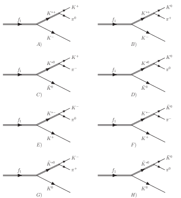
Figure 1: Tree level diagrams representing the process $f_{1}(1285)\to\pi K\bar{K}$.

II.1 Decay amplitude at tree level

In order to evaluate the partial decay width of $f_{1}(1285)\to\pi K\bar{K}$, we need the decay amplitudes of the tree level diagrams shown in Fig. 1, where the process is described as the $f_{1}(1285)$ decaying to $K^{*}\bar{K}-cc$ and then the $K^{*}$ decaying into $K\pi$. As mentioned above, the $f_{1}(1285)$ results as dynamically generated from the interaction of $K^{*}\bar{K}-c.c.$. We can write the $f_{1}(1285)K^{*}\bar{K}$ vertex as

$$-it_{1}=-ig_{f_{1}}C_{1}\epsilon^{\mu}\epsilon^{\prime}_{\mu},$$ (1)

where $\epsilon$ is the polarization vector of the $f_{1}(1285)$ state and $\epsilon^{\prime}$ is the polarization vector of the $K^{*}$ ($\bar{K}^{*}$). The $g_{f_{1}}$ is the coupling constant of the $f_{1}(1285)$ to the $K^{*}\bar{K}-cc$ channel and can be obtained from the residue in the pole of the scattering amplitude for $\bar{K}K^{*}-c.c.$ in $I=0$. We take $g_{f_{1}}=7555$ MeV in the present calculation as it comes when the pole of the $f_{1}$ is made to appear at the nominal mass of the $f_{1}(1285)$ resonance. This result is in line but a bit bigger than the value of $7230$ MeV found in Ref. roca , where a global fit to the axial vectors was conducted.  We shall take the results with these two couplings as a measure of the theoretical uncertainties. Besides, the factors $C_{1}$ account for the weight of each $K^{*}\bar{K}$ ($\bar{K}^{*}K$) component in the $I=0$ and $C=+$ combination of $K^{*}\bar{K}$ mesons, which is represented by

$$\frac{1}{\sqrt{2}}(K^{*}\bar{K}-\bar{K}^{*}K) = -\frac{1}{2}(K^{*+}K^{-}+K^{*0}\bar{K}^{0}$$ (2)

$$-K^{*-}K^{+}-\bar{K}^{*0}K^{0})\ .$$

We take the convention $CK^{*}=-\bar{K}^{*}$, which is consistent with the standard chiral Lagrangians. Then we can easily obtain the factors $C_{1}$ for each diagram shown in Fig. 1,

$$C^{A,B}_{1}=-\frac{1}{2};\ \ C^{C,D}_{1}=-\frac{1}{2};\ \ C^{E,F}_{1}=\frac{1}{2};\ \ C^{G,H}_{1}=\frac{1}{2}\ .$$ (3)

To compute the decay amplitude, we also need the structure of the $K^{*}K\pi$ vertices which can be derived using the hidden gauge symmetry Lagrangian describing the vector-pseudoscalar-pseudoscalar ($VPP$) interaction hidden1 ; hidden2 ; hidden3 ; hidden4 , given by

$${\cal L}_{VPP}=-ig<V^{\mu}[P,\partial_{\mu}P]>\ ,$$ (4)

where $g=\frac{m_{V}}{2f}$ with $m_{V}\approx m_{\rho}$ and $f=93$ MeV the pion decay constant. The symbol $<>$ stands for the trace in $SU(3)$, while the $P$ and $V$ matrices contain the nonet of pseudoscalar and vector mesons, respectively.

From the Lagrangian of Eq. (4), the vertex of $K^{*}K\pi$ can be written as

$$-it_{2}=igC_{2}(k-p)^{\mu}\epsilon^{\prime}_{\mu},$$ (5)

where $k$ and $p$ are the momenta of $\pi$ and $K$ mesons, respectively. From Eq. (4) and from the explicit expressions of the $P$ and $V$ matrices, the factors $C_{2}$ for each diagram shown in Fig. 1 can be obtained,

$$C^{A,H}_{2}=\frac{1}{\sqrt{2}};\ \ C^{B,C}_{2}=1;\ \ C^{D,E}_{2}=-\frac{1}{\sqrt{2}};\ \ C^{F,G}_{2}=-1.$$ (6)

We can now sum the amplitudes of the diagrams that have same final state. By means of Eqs. (1) and (5) and taking into account the values of $C_{1}$ and $C_{2}$, the decay amplitude is obtained straightforwardly:

$$\begin{split}&M_{\rm tree}^{A+E}=M_{\rm tree}^{D+H}=M_{\rm tree}\ ,\\ &M_{\rm tree}^{B+G}=M_{\rm tree}^{C+F}=\sqrt{2}M_{\rm tree}\ ,\end{split}$$ (7)

with

$$M_{\rm tree} = \frac{gg_{f_{1}}}{2\sqrt{2}}\big{(}[-(k-p)_{\mu}+\frac{m^{2}_{\pi}-m^{2}_{K}}{m^{2}_{K^{*}}}(k+p)_{\mu}]D_{1}$$ (8)

$$+ [-(k-p^{\prime})_{\mu}+\frac{m^{2}_{\pi}-m^{2}_{K}}{m^{2}_{K^{*}}}(k+p^{\prime})_{\mu}]D_{2}\big{)}\epsilon^{\mu}$$

$$= \frac{gg_{f_{1}}}{2\sqrt{2}}\big{(}[(\vec{k}-\vec{p})-\frac{m^{2}_{\pi}-m^{2}_{K}}{m^{2}_{K^{*}}}(\vec{k}+\vec{p})]D_{1}$$

$$+ [(\vec{k}-\vec{p^{\prime}})+\frac{m^{2}_{\pi}-m^{2}_{K}}{m^{2}_{K^{*}}}(\vec{k}+\vec{p^{\prime}})]D_{2}\big{)}\cdot\vec{\epsilon},$$

where

$$D_{1} = \frac{1}{(k+p)^{2}-m^{2}_{K^{*}}+im_{K^{*}}\Gamma_{K^{*}}},$$ (9)

$$D_{2} = \frac{1}{(k+p^{\prime})^{2}-m^{2}_{K^{*}}+im_{K^{*}}\Gamma_{K^{*}}}\ .$$ (10)

Taking diagrams A) and E) for reference to calculate $M_{\rm tree}$, the variables $p$, $p^{\prime}$ and $k$ refer to the $K^{+}$, $K^{-}$ and $\pi^{0}$, and $\Gamma_{K^{*}}$ is the total decay width of the $K^{*}$ meson.

Since the dominant decay channel of $K^{*}$ is $K\pi$, we can take

$$\Gamma_{K^{*}}=\Gamma_{\rm on}\left(\frac{q_{\rm on}}{q_{\rm off}}\right)^{3},$$ (11)

with $\Gamma_{\rm on}=49.1$ MeV, and

$$q_{\rm on} = \frac{\lambda^{1/2}(M^{2}_{K^{*}},m^{2}_{K},m^{2}_{\pi})}{2M_{K^{*}}},$$ (12)

$$q_{\rm off} = \frac{\lambda^{1/2}(M^{2}_{\rm inv},m^{2}_{K},m^{2}_{\pi})}{2M_{\rm inv}}\theta(M_{\rm inv}\!-m_{K}\!-m_{\pi}),$$ (13)

where $\lambda$ is the Källen function, with $\lambda(x,y,z)=(x-y-z)^{2}-4yz$, and $M_{\rm inv}$ is the invariant mass of the $\pi K$ system, which is $\sqrt{(k+p)^{2}}$ for the $D_{1}$ propagator and $\sqrt{(k+p^{\prime})^{2}}$ for $D_{2}$.

II.2 Decay amplitude for the triangular loop

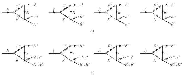
Figure 2: Triangular loop contributions to the $f_{1}(1285)\to\pi K\bar{K}$ decay.

In addition to the tree level diagrams shown in Fig. 1, we study also the contributions of the $K\bar{K}$ and $\pi K$ FSIs. We use the triangular mechanism contained in the diagrams shown in Fig. 2, consisting in the rescattering of the $K\bar{K}$ and $\pi K$ pairs. Since the $f_{1}(1285)$ has $I=0$, considering only isospin conserving terms, the $K\bar{K}$ will be in $I=1$ and the $\pi K$ in $I=1/2$. The rescattering of the $K\bar{K}$ and $\pi K$ pairs with this isospin dynamically generates in coupled channels the $a_{0}(980)$ and $\kappa(800)$ resonances, respectively. We write for simplicity the $K\bar{K}\to K\bar{K}$ and $\pi K\to\pi K$ rescattering amplitudes as,

$$t^{K\bar{K}}_{\rm FSI}(M_{K\bar{K}}) = t^{I=1}_{K\bar{K}\to K\bar{K}}(M_{K\bar{K}}),$$ (14)

$$t^{\pi K}_{\rm FSI}(M_{\pi K}) = t^{I=1/2}_{\pi K\to\pi K}(M_{\pi K}),$$ (15)

where $M_{K\bar{K}}$ and $M_{\pi K}$ are the invariant masses for the $K\bar{K}$ and $\pi K$ systems, respectively. The quantities $t^{I=1}_{K\bar{K}\to K\bar{K}}$ and $t^{I=1/2}_{\pi K\to\pi K}$ stand for the scattering amplitudes of $K\bar{K}\to K\bar{K}$ in $I=1$ and $\pi K\to\pi K$ in $I=1/2$, respectively, and they can be obtained using the Bethe-Salpeter equation

$$t=(1-VG)^{-1}V,$$ (16)

with the potential $V$ taken from Ref. npa . The $G$ function in the above equation is the loop function for the propagators of the intermediate particles

$$G(P^{2})=\int\frac{d^{4}q}{(2\pi)^{4}}\frac{1}{q^{2}-m^{2}_{1}+i\epsilon}\frac{1}{(P-q)^{2}-m^{2}_{2}+i\epsilon},$$ (17)

where $P$ is the total four-momentum ($s=P^{2}$ is the invariant mass square of the two particles in the loop) and $m_{1}$, $m_{2}$ the masses of the particles in the considered channel. We take $K\bar{K}$ and $\pi\eta$ channels for the case of $K\bar{K}$ FSI, while for $\pi K$ FSI, we take $\pi K$ and $\eta K$ channels. After the regularization by means of a cutoff npa , we obtain

$$G(s)=\int_{|\vec{q}|<q_{\rm max}}\frac{d^{3}q}{(2\pi)^{3}}\frac{\omega_{1}+\omega_{2}}{2\omega_{1}\omega_{2}}\frac{1}{s-(\omega_{1}+\omega_{2})^{2}+i\epsilon},$$ (18)

with $\omega_{i}=\sqrt{|\vec{q}|^{2}+m^{2}_{i}}$. For a good description of $a_{0}(980)$ and $\kappa(800)$ we take a cutoff $q_{\rm max}=900$ MeV, for both $K\bar{K}$ and $\pi K$ FSIs.

With the ingredients given above, we can explicitly write the decay amplitude for the diagrams in Fig. 2. As for the tree level case, we sum the diagrams with the same final state. In Fig. 2 A), we show the four possible final states for the $K\bar{K}$ FSI. The amplitude corresponding to the first diagram, that is the $\pi^{0}K^{+}K^{-}$ final state, is then given by

$$M^{K\bar{K}}_{\rm FSI}=-\frac{gg_{f_{1}}}{2\sqrt{2}}(2I_{1}+I_{2})2t^{I=1}_{K\bar{K}\to K\bar{K}}(M_{K\bar{K}})\vec{\epsilon}\cdot\vec{k},$$ (19)

with $M_{K\bar{K}}=\sqrt{(p+p^{\prime})^{2}}$. Here we have summed explicitly the contributions of four diagrams corresponding to the intermediate states $K^{*}K\bar{K}$: $K^{*+}K^{-}K^{+}$, $K^{*0}\bar{K}^{0}K^{0}$, $K^{*-}K^{+}K^{-}$ and $\bar{K}^{*0}K^{0}\bar{K}^{0}$, easily done taking into account the $C_{1}$ and $C_{2}$ coefficients and the fact that

$$t^{I=1}_{K\bar{K}\to K\bar{K}} = t_{K^{+}K^{-}\to K^{+}K^{-}}-t_{K^{+}K^{-}\to K^{0}\bar{K}^{0}}$$ (20)

$$= t_{K^{0}\bar{K}^{0}\to K^{0}\bar{K}^{0}}-t_{K^{+}K^{-}\to K^{0}\bar{K}^{0}},$$

with the phase convention $|K^{-}\rangle=-|1/2,-1/2\rangle$. The quantities $I_{1}$ and $I_{2}$ for the case of $M^{K\bar{K}}_{\rm FSI}$ are given by

$$I_{1} = -\int\frac{d^{3}q}{(2\pi)^{3}}\frac{1}{8\omega(q)\omega^{\prime}(q)\omega^{*}(q)}\frac{1}{k^{0}-\omega^{\prime}(q)-\omega^{*}(q)+i\epsilon}\frac{1}{P^{0}-\omega^{*}(q)-\omega(q)+i\epsilon}$$ (21)

$$\times\frac{2P^{0}\omega(q)+2k^{0}\omega^{\prime}(q)-2(\omega(q)+\omega^{\prime}(q))(\omega(q)+\omega^{\prime}(q)+\omega^{*}(q))}{(P^{0}-\omega(q)-\omega^{\prime}(q)-k^{0}+i\epsilon)(P^{0}+\omega(q)+\omega^{\prime}(q)-k^{0}-i\epsilon)},$$

$$I_{2} = -\int\frac{d^{3}q}{(2\pi)^{3}}\frac{\vec{k}\cdot\vec{q}/|\vec{k}|^{2}}{8\omega(q)\omega^{\prime}(q)\omega^{*}(q)}\frac{1}{k^{0}-\omega^{\prime}(q)-\omega^{*}(q)+i\epsilon}\,\frac{1}{P^{0}-\omega^{*}(q)-\omega(q)+i\epsilon}$$ (22)

$$\times\frac{2P^{0}\omega(q)+2k^{0}\omega^{\prime}(q)-2(\omega(q)+\omega^{\prime}(q))(\omega(q)+\omega^{\prime}(q)+\omega^{*}(q))}{(P^{0}-\omega(q)-\omega^{\prime}(q)-k^{0}+i\epsilon)(P^{0}+\omega(q)+\omega^{\prime}(q)-k^{0}-i\epsilon)},$$

where $\omega(q)=\sqrt{\vec{q}^{~{}2}+m^{2}_{K}}$, $\omega^{\prime}(q)=\sqrt{(\vec{q}+\vec{k})^{2}+m^{2}_{K}}$, and $\omega^{*}(q)=\sqrt{\vec{q}^{~{}2}+m^{2}_{K^{*}}}$ are the energies of the $K$ ($\bar{K}$), $\bar{K}$ ($K$), and $K^{*}$ in the triangular loop, respectively. A more detailed derivation can be found in Ref. jorgifran .

It is worth mentioning that after performing the integrations, the $I_{1}$ and $I_{2}$ integrals in the above equations depend only on the modulus of the momentum of the $\pi^{0}$, which can be easily related to the invariant mass of the $K\bar{K}$ system via $M^{2}_{K\bar{K}}=M^{2}_{f_{1}}+m^{2}_{\pi}-2M_{f_{1}}\sqrt{|\vec{k}|^{2}+m^{2}_{\pi}}$. The $d^{3}q$ integrations are done with a cutoff $q_{\rm max}=900$ MeV.

In the group B) of diagrams in Fig. 2, we show the possible final states corresponding to the $\pi K$ FSI. Each one of the diagrams has two possible $\pi\bar{K}$ or $\pi K$ final states. In addition, each one of the diagrams has two possible $K^{*}\bar{K}$ or $\bar{K}^{*}K$ intermediate states: in the first diagram we can have $K^{*+}K^{-}$ or $K^{*0}\bar{K}^{0}$ and this leads, after considering the $C_{1}$ and $C_{2}$ coefficients to the combination $t_{\pi^{0}K^{-}\rightarrow\pi^{0}K^{-}}+\sqrt{2}t_{\pi^{-}K^{0}\rightarrow\pi^{0}K^{-}}$, proportional to the $t^{I=1/2}_{\pi K\rightarrow\pi K}$. The sum of the first and third diagram with $\pi^{0}K^{+}K^{-}$ in the final state is then easily done and can be cast as

$$\begin{split}M^{\pi K}_{\rm FSI}&=\frac{gg_{f_{1}}}{2\sqrt{2}}(2I_{1}^{\prime}+I_{2}^{\prime})t^{I=1/2}_{\pi K\to\pi K}(M^{(1)}_{\pi K})\vec{\epsilon}\cdot\vec{p}\\ &+\frac{gg_{f_{1}}}{2\sqrt{2}}(2I_{1}^{\prime\prime}+I_{2}^{\prime\prime})t^{I=1/2}_{\pi K\to\pi K}(M^{(2)}_{\pi K})\vec{\epsilon}\cdot\vec{p^{\prime}},\end{split}$$ (23)

where now $I_{1}^{\prime}$, $I_{2}^{\prime}$ are evaluated with Eqs. (21) and (22) replacing one kaon propagator by a pion and simply putting $\omega^{\prime}(q)=\sqrt{(\vec{q}+\vec{p})^{2}+m_{\pi}^{2}}$ and substituting $k^{0}$ by $p^{0}$. Similarly $I_{1}^{\prime\prime}$ and $I_{2}^{\prime\prime}$ are also evaluated with Eqs. (21) and (22) putting $\omega^{\prime}(q)=\sqrt{(\vec{q}+\vec{p}^{\ \prime})^{2}+m_{\pi}^{2}}$ and substituting $k^{0}$ by $p^{\prime 0}$. The integrals $I_{1}^{\prime}$, $I_{2}^{\prime}$ are functions of $|\vec{p}|$ and $I_{1}^{\prime\prime}$, $I_{2}^{\prime\prime}$ of $|\vec{p}^{\ \prime}|$, which can be written in terms of the invariant masses $M_{\pi K}^{(1)}=\sqrt{(k+p^{\prime})^{2}}$ and $M_{\pi K}^{(2)}=\sqrt{(k+p)^{2}}$ respectively, similarly as done before for the $K\bar{K}$ interaction terms.

The relative minus sign between Eqs. (19) and (23) is easily traced back to the sign of the $K^{*}\to K\pi$ when we have either the $K$ or the $\pi$ in the loop.

III Numerical results

With the decay amplitudes obtained above, we can easily get the total decay width of $f_{1}(1285)\to\pi K\bar{K}$ which is

$$\begin{split}\Gamma&=6\frac{1}{64\pi^{3}M_{f_{1}}}\int\int d\omega_{K^{+}}d\omega_{K^{-}}\overline{\sum}|M|^{2}\\ &\times\theta(1-{\rm cos}^{2}\theta_{K\bar{K}})\theta(M_{f_{1}}-\omega_{K^{+}}-\omega_{K^{-}}-m_{\pi}),\end{split}$$ (24)

where $M$ is the full amplitude of the process $f_{1}(1285)\rightarrow\pi^{0}K^{+}K^{-}$ including the FSIs,

$$M=M_{\rm tree}+M^{K\bar{K}}_{\rm FSI}+M^{\pi K}_{\rm FSI},$$ (25)

with $M_{f_{1}}=1281.9$ MeV the mass of $f_{1}(1285)$ state and $\omega_{K^{+}}=\sqrt{m^{2}_{K}+\vec{p}^{~{}2}}$ and $\omega_{K^{-}}=\sqrt{m^{2}_{K}+\vec{p^{\prime}}^{~{}2}}$ the energies of the $K^{+}$ and $K^{-}$ mesons, respectively. The symbol $\overline{\sum}$ stands for the average over the polarizations of the initial $f_{1}(1285)$ state. The factor 6 in the formula of $\Gamma$ accounts for the different final charges for $\pi K\bar{K}$: $\pi^{0}K^{+}K^{-}$, $\pi^{+}K^{0}K^{-}$, $\pi^{-}K^{+}\bar{K}^{0}$, and $\pi^{0}K^{0}\bar{K}^{0}$, having weights 1, 2, 2, and 1, respectively, which can be easily obtained using simple Clebsch-Gordan coefficients. Besides, the ${\rm cos}\theta_{K\bar{K}}$ is defined by energy conservation as

$${\rm cos}\theta_{K\bar{K}} = \frac{1}{2|\vec{p}||\vec{p}^{\ \prime}|}[M^{2}_{f_{1}}+2m^{2}_{K}-2M_{f_{1}}(\omega_{K^{+}}+\omega_{K^{-}})$$ (26)

$$+2\omega_{K^{+}}\omega_{K^{-}}-m^{2}_{\pi}].$$

With the full amplitude of Eq. (25), the numerical result for the partial decay width is, using $g_{f1}=7555$ MeV, $\Gamma=1.9$ MeV, which corresponds to a branching ratio

$$B.R.[f_{1}(1285)\to\pi K\bar{K}]=7.8\%.$$ (27)

If we use the coupling of Ref. roca , $g_{f1}=7230$ MeV, then we get $\Gamma=1.74$ MeV, corresponding to a branching ratio

$$B.R.[f_{1}(1285)\to\pi K\bar{K}]=7.2\%.$$ (28)

This gives a band of theoretical results of

$$B.R.[f_{1}(1285)\to\pi K\bar{K}]=(7.2-7.8)\%,$$ (29)

which is in fair agreement with the experimental value: $(9.0\pm 0.4)\%$ pdg ; Barberis:1997vf ; Barberis:1998by . The result would be $9.1\%$, with the big $g_{f1}$ coupling, if we considered only the tree level diagrams. This indicates that the contribution from the FSIs is small. This occurs because of the relative minus sign in Eqs. (19) and (23), which makes the effects of the FSIs for $K\bar{K}$ and $\pi K$ go in opposite directions bringing a partial cancelation in $\Gamma$.

We should take into account that in order to get the $f_{1}(1285)$ state, cut offs of the order of $1000$ MeV in the $G$ function of $\bar{K}K^{*}$ are used. On the other hand for the $G$ function of $K\bar{K}$ and $\pi K$ a cut off of $900$ MeV was used. In the triangular loop function of Fig. 2 we have then $\theta(1000-|\vec{q}|)~{}\theta(900-|\vec{q}|)=\theta(900-|\vec{q}|)$ (in MeV). This justifies the choice of $q_{\rm max}$ in that loop function. We can see the variation of our results by changing these cut offs in a range such that the masses of the $f_{1}(1285)$ and $a_{0}(980)$ are not much changed with respect to the experimental values. In this sense, changes of $q_{\rm max}$ from $980$ MeV to 1040 MeV bring changes in the mass of the $f_{1}(1285)$ by $12$ MeV and only $1\%$ changes in the couplings. These changes are smaller than the range of couplings accepted in Eq. (29). Similarly, changes in $q_{\rm max}$ for $a_{0}(980)$ from $860$ MeV to $940$ MeV change the mass of the $a_{0}(980)$ in $7$ MeV. Reevaluating the branching ratios with values of $q_{\rm max}$ within this range, change the result that we quote in Eq. (29) to

$$B.R.[f_{1}(1285)\to\pi K\bar{K}]=(7.2-8.3)\%,$$ (30)

with the upper limit a little closer to the experimental value.

Next, we study the invariant mass distribution of the $f_{1}(1285)\to\pi^{0}K^{+}K^{-}$ decay to see the effect of the $K^{*}$ propagator in the tree level and of the $K\bar{K}$ and $\pi K$ FSIs.

The invariant mass distributions are given by the formulas

$$\frac{d\Gamma}{dM_{K^{+}K^{-}}} = \frac{M_{K^{+}K^{-}}}{64\pi^{3}M^{2}_{f_{1}}}\int d\omega_{K^{+}}\overline{\sum}|M|^{2}\theta(1-{\rm cos}^{2}\theta_{K\bar{K}})\times$$ (31)

$$\!\!\!\!\!\theta(M_{f_{1}}-\omega_{K^{+}}-\omega_{K^{-}}-m_{\pi})\theta(\omega_{K^{-}}-m_{K}),$$

$$\frac{d\Gamma}{dM_{\pi^{0}K^{+}}} = \frac{M_{\pi^{0}K^{+}}}{64\pi^{3}M^{2}_{f_{1}}}\int d\omega_{K^{+}}\overline{\sum}|M|^{2}\theta(1-{\rm cos}^{2}\theta_{K\bar{K}})\times$$ (32)

$$\!\!\!\!\!\theta(M_{f_{1}}-\omega_{K^{+}}-\omega_{K^{-}}-m_{\pi})\theta(\omega_{K^{-}}-m_{K}),$$

where

$$\omega_{K^{-}}=\frac{1}{2M_{f_{1}}}(M^{2}_{K^{+}K^{-}}+M^{2}_{f_{1}}-m^{2}_{\pi})-\omega_{K^{+}},$$ (33)

for $\frac{d\Gamma}{dM_{K^{+}K^{-}}}$, while

$$\omega_{K^{-}}=\frac{1}{2M_{f_{1}}}(M^{2}_{f_{1}}+m^{2}_{K}-M^{2}_{\pi^{0}K^{+}}),$$ (34)

for $\frac{d\Gamma}{dM_{\pi^{0}K^{+}}}$.

The results for $\frac{d\Gamma}{dM_{K^{+}K^{-}}}$ and $\frac{d\Gamma}{dM_{\pi^{0}K^{+}}}$ are shown in Fig. 3 and Fig. 4, respectively. It is very interesting to compare the different curves in Figs. 3 and 4. We show there the results assuming just a phase space distribution ($\overline{\sum}|M|^{2}$ in Eqs. (31) and (32) is set to a constant), and with the tree level or tree level plus final state interaction of $K\bar{K}$ and $\pi K$. For the sake of comparison, the curves are normalized to the same $\Gamma$. In Fig. 3 we see that the tree level alone shows a distinct shape, very different from phase space, with a peak at low $M_{K^{+}K^{-}}$. This must be attributed to the effect of the $K^{*}$ off shell propagator. The implementation of FSI, particularly the $K\bar{K}$ in this case, is responsible for a further shift of the mass distribution to lower invariant masses, closer to the $K\bar{K}$ threshold, where the $a_{0}(980)$ resonance appears.

Figure 3: The mass distribution $\frac{d\Gamma}{dM_{K^{+}K^{-}}}$ for $f_{1}(1285)\to\pi^{0}K^{+}K^{-}$ as a function of the invariant mass of the $K^{+}K^{-}$ system.

In Fig. 4, where the $\pi K$ invariant mass distribution is plotted, we see a similar behaviour. The tree level alone already produces a shape quite different from phase space, with a peak at high values of $M_{\pi K}$, to be attributed once again to the off shell $K^{*}$ propagator. The implementation of FSI, particularly the $\pi K$ in this case, pushes the peak of the mass distributions to higher $M_{\pi K}$, closer to the region where the $\kappa(800)$ resonance appears.

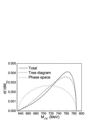
Figure 4: The mass distribution $\frac{d\Gamma}{dM_{\pi^{0}K^{+}}}$ for $f_{1}(1285)\to\pi^{0}K^{+}K^{-}$ as a function of the invariant mass of the $\pi^{0}K^{+}$ system.

The two figures show how the most drastic change in the shape of the two mass distributions is already caused by the tree level alone and, as mentioned before, this is tied to the $K^{*}$ propagators, which appears at tree level because of the $\bar{K}^{*}K-cc$ nature of the $f_{1}(1285)$ state that we have assumed. These mass distributions have not been measured yet and it is clear from the present study that their observation would be very important to determine the nature of this resonance.

So far we have assumed that the $f_{1}(1285)$ resonance is fully made from $K\bar{K}^{*}$. There are hints that the resonance could have also other components. Indeed, in the study of this resonance in finite volume gengfinite it was shown that applying the compositeness sum rule hyodo1 ; hyodo2 ; sekihara to this case with the chiral potential, the $K\bar{K}^{*}$ molecular component accounted for about $50\%$ of the probability of the wave function, but there could still be a sizable fraction for other non $K\bar{K}^{*}$ components. The size of these components is uncertain because it relies on the energy dependence contained in the chiral potential and it is unclear that this accounts for missing channels (see Ref. acetidelta ), but it really hints at the possibility to have some non negligible non $K\bar{K}^{*}$ molecular component in the $f_{1}(1285)$ wave function. This might seem to be in conflict with our claims of a basically molecular state for this resonance. This requires some explanation. Different parts of the wave function revert in different ways on certain observables. The easiest such case is the nucleon form factor, which at low momentum transfer is dominated by the meson baryon components of the nucleon, while at high momentum transfers it is the core of quarks that is responsible for it thomasrep ; ulfrep . In this sense, it is logical that the decay of the $f_{1}(1285)$ into $K\bar{K}\pi$ and related channels is mostly due to the $K\bar{K}^{*}$ molecular component of the wave function, and other components would show up in other reactions. In this sense it is interesting to note that in Ref. sheldons the $B^{0}$ and $B^{0}_{s}$ decays into $J/\psi$ and $f_{1}(1285)$ are investigated and the interpretation in terms of a $q\bar{q}$ state leads to a $f_{1}(1285)$ state mostly made of $u$ and $d$ quarks. In our case we have four quarks to start with and a sizable fraction of strange quarks in our $K\bar{K}^{*}$ molecular component, so the models seem to be contradictory. Yet, one must recall that in this latter case we have production of the resonance in $B$ decays and the resonance must be formed starting from a $q\bar{q}$ component. The investigation done in Refs. liang ; liangmela of the $B$ decays, and the ratio of the rates of $\bar{B}^{0}\to J/\psi f_{0}(500)$ Aaij:2013zpt and $\bar{B}^{0}\to J/\psi\rho$ pdg , show that the hadronization of the primary $q\bar{q}$ component to give two mesons has a penalty factor that reverts into a factor of $0.37$ decrease in the partial decay width. In this sense, the decays of heavy mesons leading to light ones might reveal themselves into a source of information on the non molecular components of states like the present one. Further research considering both the molecular and $q\bar{q}$ components for this resonance in the $B$ decays would be most welcome after the discussion made here.

IV Summary

In this work, we evaluate the partial decay width of the $f_{1}(1285)\to\pi K\bar{K}$ with the assumption that the $f_{1}(1285)$ is dynamically generated from the $\bar{K}^{*}K-cc$ interaction. The tree level diagrams proceeding via $f_{1}(1285)\to K^{*}\bar{K}-cc\to\pi K\bar{K}$ are considered. Besides, we also take into account the final state interactions of $K\bar{K}\to K\bar{K}$ and $\pi K\to\pi K$. It is found that the contributions from the FSIs are small compared to the tree level diagrams to the partial decay width, but they change the mass distributions of the $f_{1}(1285)\to\pi K\bar{K}$ decay.

The result that we obtained for the width is compatible with experiment within errors. Yet, we find some relevant features in the $K\bar{K}$ and $\pi K$ mass distributions, which turn out to be very different from phase space. The FSI is partly responsible for the shapes obtained but we found that the tree level contribution, which is dominant in the process, is mostly responsible for this different shape, which must be attributed to the off shell $K^{*}$ propagator appearing in the process under the assumption that the $f_{1}(1285)$ is a $K^{*}\bar{K}-cc$ molecule. The experimental observations of those mass distributions would then provide very valuable information on the relevance of this component in the $f_{1}(1285)$ wave function.

References

- [1] M. C. Birse, Z. Phys. A 355, 231 (1996).
- [2] M. Bando, T. Kugo, S. Uehara, K. Yamawaki and T. Yanagida, Phys. Rev. Lett. 54, 1215 (1985).
- [3] M. Bando, T. Kugo and K. Yamawaki, Phys. Rept. 164, 217 (1988).
- [4] M. Harada and K. Yamawaki, Phys. Rept. 381, 1 (2003).
- [5] U. G. Meissner, Phys. Rept. 161, 213 (1988).
- [6] M. F. M. Lutz and E. E. Kolomeitsev, Nucl. Phys. A 730, 392 (2004).
- [7] L. Roca, E. Oset and J. Singh, Phys. Rev. D 72, 014002 (2005).
- [8] A. Faessler, T. Gutsche, S. Kovalenko and V. E. Lyubovitskij, Phys. Rev. D 76, 014003 (2007).
- [9] A. Faessler, T. Gutsche, V. E. Lyubovitskij and Y. L. Ma, Phys. Rev. D 76, 114008 (2007).
- [10] C. Garcia-Recio, L. S. Geng, J. Nieves and L. L. Salcedo, Phys. Rev. D 83, 016007 (2011).
- [11] H. Nagahiro, K. Nawa, S. Ozaki, D. Jido and A. Hosaka, Phys. Rev. D 83, 111504 (2011).
- [12] F. K. Guo, P. N. Shen and H. C. Chiang, Phys. Lett. B 647, 133 (2007).
- [13] D. Gamermann and E. Oset, Eur. Phys. J. A 33, 119 (2007).
- [14] F. K. Guo, C. Hanhart and U. G. Meissner, Eur. Phys. J. A 40, 171 (2009).
- [15] M. Altenbuchinger, L.-S. Geng and W. Weise, Phys. Rev. D 89, no. 1, 014026 (2014).
- [16] C. B. Lang, L. Leskovec, D. Mohler, S. Prelovsek and R. M. Woloshyn, Phys. Rev. D 90, 034510 (2014).
- [17] A. M. Torres, E. Oset, S. Prelovsek and A. Ramos, JHEP 1505, 153 (2015).
- [18] Y. Zhou, X. L. Ren, H. X. Chen and L. S. Geng, Phys. Rev. D 90, no. 1, 014020 (2014).
- [19] L. S. Geng, X. L. Ren, Y. Zhou, H. X. Chen and E. Oset, Phys. Rev. D 92, no. 1, 014029 (2015).
- [20] F. Aceti, J. M. Dias and E. Oset, Eur. Phys. J. A 51, no. 4, 48 (2015).
- [21] J. A. Oller and E. Oset, Nucl. Phys. A 620, 438 (1997) [Erratum-ibid. A 652, 407 (1999)].
- [22] J. A. Oller, E. Oset and J. R. Pelaez, Phys. Rev. D 59, 074001 (1999) [Erratum-ibid. D 60, 099906 (1999)] [Erratum-ibid. D 75, 099903 (2007)].
- [23] N. Kaiser, Eur. Phys. J. A 3, 307 (1998).
- [24] M. P. Locher, V. E. Markushin and H. Q. Zheng, Eur. Phys. J. C 4, 317 (1998).
- [25] J. Nieves and E. Ruiz Arriola, Nucl. Phys. A 679, 57 (2000).
- [26] J. R. Pelaez and G. Rios, Phys. Rev. Lett. 97, 242002 (2006).
- [27] M. Ablikim et al. [BESIII Collaboration], Phys. Rev. D 92, no. 1, 012007 (2015).
- [28] E. van Beveren, T. A. Rijken, K. Metzger, C. Dullemond, G. Rupp and J. E. Ribeiro, Z. Phys. C 30 (1986) 615.
- [29] N. A. Tornqvist and M. Roos, Phys. Rev. Lett. 76 (1996) 1575.
- [30] A. H. Fariborz, R. Jora and J. Schechter, Phys. Rev. D 79, 074014 (2009).
- [31] A. H. Fariborz, N. W. Park, J. Schechter and M. Naeem Shahid, Phys. Rev. D 80, 113001 (2009).
- [32] K. A. Olive et al. [Particle Data Group Collaboration], Chin. Phys. C 38, 090001 (2014).
- [33] D. Gamermann, E. Oset, D. Strottman and M. J. Vicente Vacas, Phys. Rev. D 76, 074016 (2007).
- [34] M. Ablikim et al. [BESIII Collaboration], Phys. Rev. Lett. 108, 182001 (2012).
- [35] J. J. Wu, X. H. Liu, Q. Zhao and B. S. Zou, Phys. Rev. Lett. 108, 081803 (2012).
- [36] F. Aceti, W. H. Liang, E. Oset, J. J. Wu and B. S. Zou, Phys. Rev. D 86, 114007 (2012).
- [37] N. N. Achasov, A. A. Kozhevnikov and G. N. Shestakov, Phys. Rev. D 92, no. 3, 036003 (2015).
- [38] K. Chen, C. Q. Pang, X. Liu and T. Matsuki, Phys. Rev. D 91, no. 7, 074025 (2015) [arXiv:1501.07766 [hep-ph]].
- [39] E. Klempt and A. Zaitsev, Phys. Rept. 454, 1 (2007).
- [40] P. Gavillet, R. Armenteros, M. Aguilar-Benitez, M. Mazzucato and C. Dionisi, Z. Phys. C 16, 119 (1982).
- [41] D. M. Li, H. Yu and Q. X. Shen, Chin. Phys. Lett. 17, 558 (2000).
- [42] J. Vijande, F. Fernandez and A. Valcarce, J. Phys. G 31, 481 (2005).
- [43] S. Godfrey and J. Napolitano, Rev. Mod. Phys. 71, 1411 (1999).
- [44] R. Aaij et al. [LHCb Collaboration], Phys. Rev. Lett. 112, no. 9, 091802 (2014).
- [45] D. Barberis et al. [WA102 Collaboration], Phys. Lett. B 413, 225 (1997).
- [46] D. Barberis et al. [WA102 Collaboration], Phys. Lett. B 440, 225 (1998).
- [47] T. Hyodo, D. Jido and A. Hosaka, Phys. Rev. C 85, 015201 (2012).
- [48] T. Hyodo, Int. J. Mod. Phys. A 28, 1330045 (2013).
- [49] T. Sekihara, T. Hyodo and D. Jido, PTEP 2015, no. 6, 063D04.
- [50] F. Aceti, L. R. Dai, L. S. Geng, E. Oset and Y. Zhang, Eur. Phys. J. A 50, 57 (2014).
- [51] A. W. Thomas, Ad. Nucl. Phys. 13, 1 (1984).
- [52] V. Bernard, N. Kaiser and U. G. Meissner, Int. J. Mod. Phys. E 4, 193 (1995).
- [53] W. H. Liang and E. Oset, Phys. Lett. B 737, 70 (2014).
- [54] M. Bayar, W. H. Liang and E. Oset, Phys. Rev. D 90, no. 11, 114004 (2014).
- [55] R. Aaij et al. [LHCb Collaboration], Phys. Rev. D 87, no. 5, 052001 (2013).