Abstract

We construct the Killing(–Yano) tensors for a large class of charged black holes in higher dimensions and study general properties of such tensors, in particular, their behavior under string dualities. Killing(–Yano) tensors encode the symmetries beyond isometries, which lead to insights into dynamics of particles and fields on a given geometry by providing a set of conserved quantities. By analyzing the eigenvalues of the Killing tensor, we provide a prescription for constructing several conserved quantities starting from a single object, and we demonstrate that Killing tensors in higher dimensions are always associated with ellipsoidal coordinates. We also determine the transformations of the Killing(–Yano) tensors under string dualities, and find the unique modification of the Killing–Yano equation consistent with these symmetries. These results are used to construct the explicit form of the Killing(–Yano) tensors for the Myers–Perry black hole in arbitrary number of dimensions and for its charged version.

1 Introduction and summary

Symmetries of dynamical equations have always played very important role in string theory. Conformal symmetry of the worldsheet led to Polyakov’s reformulation of the theory [1], making it amenable to quantization, and provided powerful tools for performing calculations [2]. Study of string dualities [3] led to great insights into dynamics of string theory at strong coupling and to formulation of the gauge/gravity duality [4]. More recently discovery of hidden symmetries of equations for a classical string led to the discovery of integrability [5, 6], which stimulated a great progress in understanding of string dynamics and gauge/gravity duality (see [7] for the review and list of references). To gain additional insights into properties of quantum gravity and strong interactions it is very important to look for new examples of integrable string backgrounds. Since at low energies strings behave as point–like particles, integrable structures must give rise to hidden symmetries of supergravity, which will be investigated in this article.

Integrability of classical strings on certain backgrounds is guaranteed by an infinite number of conserved quantities which can be extracted from reformulating the dynamical equations as a linear Lax pair [8]. Unfortunately, there is no algorithmic procedure for constructing such pairs, and they have to be guessed. Interestingly, there exists a procedure for demonstrating that a particular background does not have a Lax pair, and it has been applied in [9, 10] to rule out several promising candidates, such as strings on a conifold and on asymptotically–flat geometry produced by D3 branes. Unfortunately, this procedure for ruling out integrability is rather complicated, and it has to be applied on a case–by–case basis, so in [11] we used a different approach based on the study of geodesics. Since at low energies strings behave as point particles, integrability must survive as a hidden symmetry of such objects, and this gives a very coarse necessary condition for integrability, which can be tested for large classes of backgrounds. Interestingly, this condition was sufficient for ruling out integrability on all known supersymmetric geometries produced by D–branes, with an exception of AdS${}_{p}\times$S^q and a couple of other examples [11]. Of course, to analyze the integrability of geodesics one has to start with explicit solutions, and the nontrivial integrable deformations of AdS${}_{p}\times$S^q [12, 13] had to be constructed using special techniques rather than obtained as members of known families. This article is a continuation of the program initiated in [11]: it extends the earlier results to geometries without supersymmetry, and, more importantly, it uncovers the hidden symmetries underlying integrability of geodesics. In spite of this continuity, this paper does not require familiarity with [11].

Study of geodesics has a long history in general relativity, and the most powerful methods are based on the analysis of the Hamilton–Jacobi (HJ) equation. It is well-know that such equation separates if the background contains cyclic (ignorable) directions, but sometimes separation happens even between non–cyclic coordinates. The simplest example of such ‘accidental separation’ comes from the three–dimensional flat space in spherical coordinates: the polar angle $\theta$ separates in the HJ equation, although the metric depends on this coordinate. In this case the separation can be attributed to the SU(2) symmetries of the sphere, but similar argument cannot be applied to the Kerr black hole, which has only U(1)$\times$U(1) isometry, although the $\theta$ coordinate still separates. The technical aspects of this separation will be reviewed in section 2.2, and here we just recall that the separation is associated with a hidden symmetry encoded in the Killing tensor (KT) [15, 16]. The same tensor also leads to separation of the Klein–Gordon equation even beyond the eikonal approximation. The Kerr metric also gives rise to separable Dirac equation, this is guaranteed by an additional symmetry encoded in the Killing–Yano tensor (KYT) [17]. Over the last four decades Killing(–Yano) tensors have been found for other geometries both in general relativity [18] and in string theory [19], and in this article we will construct KYT for a large class geometries in arbitrary numbers of dimensions, which contains most of the known examples as special cases.

Killing(–Yano) tensors encode all continuous symmetries of solutions in general relativity, but string theory also has discrete symmetries associated with dualities, which can be promoted to a continuous group of solution-generating transformations in supergravity. This leads to a very natural question: what happens with Killing(–Yano) tensors under action by this group? Answering this question is one of the main goals of this paper. A slightly different question was answered in the article [20], which identified the subset of duality transformation leaving the Killing–Yano tensor invariant. As we will see, in general both Killing and Killing–Yano tensors are changed by the dualities, even the equation for the KYT is modified. However, for the special cases discussed in [20] our results agree with that paper. In this article we focus on dualities in the NS–NS sector since our preliminary study of the Ramond–Ramond backgrounds indicates that T duality applied to such geometries may change the rank of the KYT and even produce Killing–Yano tensors of mixed rank. A very brief discussion of this point is given in section 4.3.

This paper has the following organization.

In sections 2.1 and 2.3 we review some well-known properties of Killing(–Yano) tensors, and in section 2.2 we rewrite them in a slightly unusual form which becomes crucial for the subsequent discussion. Usually one uses the Killing tensor to produce a conserved quantity which leads to separation of the HJ and Klein–Gordon equations, and only one such quantity can be constructed from a given Killing tensor. In section 2.2 we argue that if one looks further and studies the eigenvalues of the Killing tensor, then a single KT can lead to a family of conserved quantities since the detailed analysis of eigenvalues allows one to construct a family of Killing tensors from a single representative using an algebraic procedure (i.e., without solving differential equations). As a bi–product of this analysis we also demonstrate that separation caused by nontrivial Killing tensors in any number of dimensions can only happen in (degenerate) ellipsoidal coordinates, this generalizes the earlier result of [11] to non–supersymmetric geometries. In section 2.3 we also show that the eigenvectors of the Killing tensors lead to simple expressions for the Killing–Yano tensors when the latter exist.

After developing this general technology we apply it in section 3 to write the Killing–Yano and Killing tensors for the Myers–Perry black holes [21] in arbitrary number of dimensions with arbitrary number of rotations. In section 5.1 this construction is extended to charged solutions built from Myers–Perry geometries by application of the solution–generating dualities, and relatively simple explicit expressions for the Killing(–Yano) tensors are derived.

The general effects of string dualities on Killing(–Yano) tensors are discussed in section 4, where it is demonstrated that Killing vectors (KV) and Killing tensors survive under dualities if certain conditions on the Kalb–Ramond field are satisfied, and the resulting transformations for the KV and KT are derived. For the Killing–Yano tensors the situation is rather different: while dualities generically destroy the standard KYT, they preserve the modified version of the KYT equation, which is derived in section 4.3. We demonstrate that such duality–invariant modification is unique and derive the transformation laws for the Killing–Yano tensor. Several examples of the modified KY tensors are discussed in section 5.

While studying massless particles, one encounters Conformal Killing(–Yano) tensors (CKT and CKYT), and their behavior under string dualities has some unusual aspects. The conformal objects are discussed throughout the paper along with their standard counterparts. Some technical details are presented in appendices.

2 Killing(–Yano) tensors in higher dimensions

2.1 Killing tensors and Killing–Yano tensors

Symmetries play very important role in physics, and symmetries of geometries are encoded in Killing vectors and Killing tensors. In this section we will review some well–known properties of these objects and establish the notation which will be used in the rest of the paper.

We begin with recalling that the Killing vector (KV) is defined as a vector field $V$ which leaves the metric invariant. In other words, the Lie derivative of the metric along $V$ must vanish:

$${\cal L}_{V}g_{MN}=0,$$ (2.1)

Relation (2.1) can be rewritten as

$${\cal L}_{V}g_{MN}=V^{P}\partial_{P}g_{MN}+\partial_{M}V^{P}g_{PN}+\partial_{N}V^{P}g_{MP}=\nabla_{M}V_{N}+\nabla_{N}V_{M}=0,$$ (2.2)

and it implies that the metric does not change under an infinitesimal transformation

$$x^{\prime M}=x^{M}+\epsilon V^{M}.$$ (2.3)

Since Killing vectors encode symmetries, they are always associated with conserved quantities. Specifically, the expression

$$I=V_{M}\frac{dx^{M}}{ds}$$ (2.4)

is conserved along any geodesic.

The correspondence between Killing vectors and integrals of motion is not one–to-one: some conserved quantities are not associated with KV. However, it was shown by Penrose and Walker [16] that any integral of motion that depends on momentum comes either from a Killing vector or from a rank–two Killing tensor as

$$I=K_{MN}\frac{dx^{M}}{ds}\frac{dx^{N}}{ds},$$ (2.5)

where $K_{MN}$ satisfies a linear equation

$$\nabla_{M}K_{NP}+\nabla_{N}K_{MP}+\nabla_{P}K_{MN}=0.$$ (2.6)

To determine whether the integrals of motion survive in quantum theory as well, one should analyze separability of the Klein–Gordon equation, and as shown in [23], the relevant conserved quantity must be associated with eigenvalues of the differential operator

$${\hat{K}}\equiv\frac{1}{\sqrt{-g}}\partial_{M}\left[\sqrt{-g}K^{MN}\partial_{N}\right]+k(x)$$ (2.7)

with some function $k(x)$. As demonstrated in [24, 23], operator ${\hat{K}}$ commutes with $\nabla_{M}\nabla^{M}$ if and only if $K^{MN}$ satisfies equation (2.6) and one more condition which will not be discussed here.

In general, presence of the Killing tensor does not imply separability of the Dirac equation, this requires existence of an anti–symmetric Killing–Yano tensor (KYT) $Y_{MN}$ which satisfies the defining equation [17]

$$\nabla_{M}Y_{NP}+\nabla_{N}Y_{MP}=0.$$ (2.8)

This equation can be generalized to tensors of arbitrary rank as [25]

$$\nabla_{(M}Y_{N)P_{1}\dots P_{k-1}}=0,\quad Y_{P_{1}\dots P_{k}}=Y_{[P_{1}\dots P_{k}]}.$$ (2.9)

In four dimensions KYT of rank $k>2$ can be dualized into vectors and scalars, but in string theory one encounters interesting solutions of (2.9), which will be discussed throughout this paper. It is also possible to define Killing tensors of rank $k>2$ as solutions of the equation [16]

$$\nabla_{(M_{1}}K_{M_{2}\dots M_{k+1})}=0,$$ (2.10)

but such objects will not play any role in our discussion.

Any KYT gives rise to a Killing tensor of rank two via the relation

$${K}_{MN}={Y}_{M}{}^{A_{1}\dots A_{k-1}}{Y}_{NA_{1}\dots A_{k-1}}.$$ (2.11)

This equation has a simple interpretation: separability of the Dirac equation implies one for the Klein–Gordon equation in the same coordinates. In section 2.2 we will present a detailed analysis of Killing tensors and outline a procedure for “extracting the square root” from them which allows one to construct the Killing–Yano tensors, if they exist.

So far we discussed the integrals of motion for massive particles, but some additional symmetries might arise in the massless case. For example, while the metric

$$ds^{2}=dr^{2}+r^{2}d\phi^{2}$$ (2.12)

is not invariant under rescaling of $r$ coordinate, massless particles are not sensitive to such rescaling, so while

$${\cal V}=r\partial_{r}$$ (2.13)

is not a Killing vector, it does lead to conserved quantities for massless particles. Such conformal Killing vectors (CKV) satisfy equation

$$\nabla_{M}{\cal V}_{N}+\nabla_{N}{\cal V}_{M}=vg_{MN},$$ (2.14)

where $v$ is an arbitrary functions of all coordinates. If $v$ is a constant, then the corresponding CKV is called homothetic [26], and such vectors will play an important role in the analysis presented in section 4.1.3.

The conformal Killing(–Yano) tensors (CKT and CKYT) are defined as solutions of equations

$$\nabla_{(M_{1}}{\cal K}_{M_{2}...M_{k+1})}=W_{(M_{1}...M_{k-1}}g_{M_{k}M_{k+1})},$$ (2.15)

$$\nabla_{(M_{1}}{\cal Y}_{M_{2})...M_{k+1}}=g_{M_{1}M_{2}}Z_{M_{3}...M_{k+1}}+\sum_{i=3}^{k+1}(-1)^{i}g_{M_{i}(M_{1}}Z_{M_{2})...{M_{i-1}}M_{i+1}...M_{k+1}}.$$

with coordinate–dependent tensors $W$ and $Z$. Notice that under rescaling of the metric, CKV, CKT and CKYT transform in a simple way, so they survive S duality and transition from the string to the Einstein frame. Ordinary Killing vectors have the same feature, as long as we impose a reasonable restriction on the dilaton:

$${\cal L}_{V}e^{2\Phi}=V^{M}\partial_{M}e^{2\Phi}=0.$$ (2.16)

On the other hand, the ordinary KT and KYT are usually destroyed by coordinate–dependent rescaling of the metric, so they exist only in one frame. Conformal transformations of the KT and KYT are discussed in Appendix A.

We will mostly focus on rank–2 KT and CKT, and they can be constructed by squaring KYT or CKYT:

$${\cal K}_{MN}={\cal Y}_{M}{}^{A_{1}\dots A_{k-1}}{\cal Y}_{NA_{1}\dots A_{k-1}},\quad W_{M}=2{\cal Y}_{MA_{1}\dots A_{k-1}}Z^{A_{1}\dots A_{k-1}}.$$ (2.17)

For rank-1 and rank–2 (C)KYT this construction is well-known, and direct computation shows that it works for all $k$.

Conformal Killing tensors ${\cal K}_{MN}$ with $W_{M}=-\nabla_{M}\phi$ have a special property: they can be extended to the standard KT $K_{MN}$ by

$$K_{MN}={\cal K}_{MV}+\phi g_{mn}.$$ (2.18)

To see this one can take a covariant derivative of (2.18) and symmetrize the result:

$$\nabla_{(M}K_{NP)}=\nabla_{(M}{\cal K}_{NP)}+\nabla_{(M}\phi g_{NP)}=0.$$ (2.19)

This construction will be illustrated in section 2.3 by comparing KT and CKT for rotating black holes.

2.2 Killing tensors and the Hamilton–Jacobi equation

Solutions of the equation for the KT,

$$\nabla_{P}K_{MN}+\nabla_{M}K_{NP}+\nabla_{N}K_{PM}=0$$ (2.20)

form a linear space, in particular, a ‘trivial subspace’ is spanned by combinations of the metric and Killing vectors,

$$K^{triv}_{MN}=e_{0}g_{MN}+\sum_{i,j}e_{ij}V^{(i)}_{M}V^{(j)}_{N},$$ (2.21)

with constant coefficients $e_{0}$, $e_{ij}$. In this subsection we will establish a one–to–one correspondence between nontrivial Killing tensors and separation of variables in the Hamilton–Jacobi equation

$$g^{MN}\partial_{M}S\partial_{N}S+\mu^{2}=0.$$ (2.22)

2.2.1 Killing tensors from the Hamilton–Jacobi equation

There are several notions of separability for equation (2.22), and we focus on the standard one by assuming that

$$S=S(x_{1},\dots x_{k})+S(x_{k+1}\dots x_{n}).$$ (2.23)

This assumption can be generalized to R–separability as

$$S=S(x_{1},\dots x_{k})+S(x_{k+1}\dots x_{n})+S_{0}(x_{1}\dots x_{n}),$$ (2.24)

where $S_{0}(x_{1}\dots x_{n})$ is a known function of its arguments [27]. However, this generalization will not play any role in our discussion.

Equation (2.22) separates as (2.23) if and only if three conditions are satisfied:

1. Coordinates $x^{M}$ can be divided into cyclic coordinates $z$ and two other groups, which will be denoted by $x$ and $y$. The metric does not depend on coordinates $z$.

2. There exists a separation function $f$, such that

   $$g^{MN}=\frac{1}{f}\left(X^{MN}+Y^{MN}\right),\quad\partial_{x}Y^{MN}=\partial_{y}X^{MN}=0,\ X^{y^{i}M}=0,\ Y^{x^{i}M}=0.$$ (2.25)

3. Function $f$ can be decomposed as

   $$f=f_{x}-f_{y},\qquad\partial_{y}f_{x}=0,\quad\partial_{x}f_{y}=0,\quad\partial_{z}f_{x}=\partial_{z}f_{y}=0.$$ (2.26)

Conditions (a)–(c) allow us to rewrite equation (2.22) as

$$X^{MN}\partial_{M}S\partial_{N}S+\mu^{2}f_{x}=-Y^{MN}\partial_{M}S\partial_{N}S+\mu^{2}f_{y},$$ (2.27)

where the left–hand side depends only on $x$, and the right–hand side depends only on $y$. This implies that

$$I\equiv\left[X^{MN}-f_{x}g^{MN}\right]\partial_{M}S\partial_{N}S$$ (2.28)

must be an integral of motion, and as such it must be associated with a Killing tensor:

$$I=K^{MN}\partial_{M}S\partial_{N}S.$$ (2.29)

We conclude that separation of variables (a)–(c) is associated with Killing tensor

$$K^{MN}=X^{MN}-\frac{f_{x}}{f}\left(X^{MN}+Y^{MN}\right)=-\frac{f_{y}X^{MN}+f_{x}Y^{MN}}{f}.$$ (2.30)

If condition (c) is not satisfied, then equation (2.22) separates only for $\mu=0$, and the associated conformal Killing tensor is

$$K^{MN}=X^{MN}.$$ (2.31)

After reviewing the standard procedure for extracting the Killing tensor from separation of variables [15, 16], we discuss the inverse problem: recovery of separation from a given Killing tensor.

2.2.2 Separation of variables from Killing tensor

Every Killing tensor gives rise to an integral of motion via (2.29), and such constant must be associated with separation of variables as in (2.28). While the separation functions $(f_{x},f_{y})$ and the corresponding tensors $(X^{MN},Y^{MN})$ are encoded in the Killing tensor, extracting them requires further analysis, and as we will demonstrate, this analysis may lead to an entire family of the Killing tensors which can be constructed algebraically from one representative. Schematically our results can be represented as

$$\begin{array}[]{c}\mbox{Eigenvalues}\\ \mbox{of KT}\end{array}\quad\Rightarrow\quad\mbox{separation}\quad\Rightarrow\quad\begin{array}[]{c}m\mbox{--parameter}\\ \mbox{family of KTs}\end{array}\,\quad\Leftrightarrow\quad\begin{array}[]{c}m\,\mbox{conserved}\\ \mbox{charges}\end{array}$$ (2.38)

To justify the usefulness of eigenvalues we recall equations (2.25) and (2.30):

$$g^{MN}=\frac{1}{f}\left(X^{MN}+Y^{MN}\right),\qquad K^{MN}=-\frac{f_{y}X^{MN}+f_{x}Y^{MN}}{f}$$ (2.39)

and consider an eigenvalue problem:

$$K^{MN}Z_{N}=\Lambda g^{MN}Z_{N}.$$ (2.40)

Assuming that metric has at least one non–cyclic direction $x$ and that there is at least one component $K^{xN}\neq 0$, the $M=x$ component of (2.40) becomes

$$-\frac{f_{y}}{f}X^{xN}Z_{N}=\Lambda\frac{1}{f}\,X^{xN}Z_{N}\quad\Rightarrow\quad\Lambda=-f_{y}.$$ (2.41)

In other words, some eigenvalues of the Killing tensor give the separation functions, and corresponding eigenvectors can be used to recover the relevant tensors $(X^{MN},Y^{MN})$. The cyclic coordinates complicate this construction, so they should be ignored to recover the separation function and added back in the end. Specifically, we propose the following procedure for extracting the separation function from the Killing tensor:

1. Find the eigenvalues and eigenvectors of the KT:

   $$K_{MN}=\sum_{a}\Lambda_{a}e^{(a)}_{M}e^{(a)}_{N},\qquad g_{MN}=\sum_{a}e^{(a)}_{M}e^{(a)}_{N}.$$ (2.42)

   Notice that some eigenvalues may vanish of be degenerate.

2. Build the projectors

   $$P^{(a)}_{MN}=e^{(a)}_{M}e^{(a)}_{N}.$$

   Projector $P$ will be called cyclic if

   $$\sum_{N}{[P^{(a)}]_{M}}^{N}\partial_{N}\Lambda_{b}=0\quad\mbox{for all}\quad(a,b).$$ (2.43)

   If all projectors are cyclic, the Killing tensor can be built from Killing vectors and the metric.

3. Remove all directions associated with cyclic projectors and construct the reduced metric and Killing tensor:

   $$K^{red}_{MN}=\left[{\sum_{a}}\Lambda_{a}e^{(a)}_{M}e^{(a)}_{N}\right]_{red},\qquad g^{red}_{MN}=\left[{\sum_{a}}e^{(a)}_{M}e^{(a)}_{N}\right]_{red}.$$

   Non–cyclic components of equation (2.20) imply that $K^{red}_{MN}$ is a Killing tensor for $g^{red}_{MN}$. Nontrivial $K^{red}_{MN}$ and $g^{red}_{MN}$ imply that Killing tensor cannot be constructed from the Killing vectors and the metric.

4. Separation of variables implies that

   $$\sum_{M}e^{(a)}_{M}dx^{M}=\sqrt{g_{a}}dx^{a},\qquad\partial_{j}\partial_{k}\ln g_{m}=0\ \mbox{for different}\ (i,j,k).$$ (2.44)

   Then analysis of the Killing equations shows that generically the reduced metric and Killing tensor must have the form

   $$ds^{2}_{red}=\sum_{k}g_{k}(dx_{k})^{2},\quad K_{red}=\sum_{k}\Lambda_{k}g_{k}(dx_{k})^{2},$$

   $$g_{k}=h_{k}(x_{k})\prod_{j\neq k}[x_{k}-x_{j}],\quad\Lambda_{j}=\partial_{j}\Lambda,$$ (2.45)

   where $\Lambda(x_{1}\dots x_{n})$ is a linear polynomial in every $(x_{1}\dots x_{n})$ symmetric under interchange of every pair of arguments.

5. Separation of variables in the reduced metric is accomplished by multiplying the reduced HJ equation by

   $$\rho_{k}=\prod_{j\neq k}[x_{k}-x_{j}].$$ (2.46)

   Then the reduced HJ equation can be written as

   $$\frac{1}{h_{k}}(\partial_{k}S)^{2}=\sum_{p=0}^{n-1}(x_{k})^{p}I^{(k)}_{p}(x_{1}\dots x_{k-1},x_{k+1}\dots x_{n}),$$ (2.47)

   which implies that all $I^{(k)}_{p}$ must be constant. This construction separates variable $x_{k}$, and other coordinates can be separated in the same fashion

6. After coordinates $(x_{1}\dots x_{n})$ have been constructed, cyclic directions can be added back, and upon multiplication by (2.46) the complete $d$–dimensional HJ equation takes the form (2.47). This follows from the fact that $K$ from (2.42) was a Killing tensor for the $d$–dimensional metric.

7. A given Killing tensor corresponds to a particular function $\Lambda$ in (4), and a family of Killing tensors for the reduced metric can be constructed by keeping the same coordinates and introducing an arbitrary polynomial $\Lambda$.

Steps (1)–(7) outline our construction, and the details and justification are presented in the Appendix B.1. A different approach to separation functions and Killing tensors was developed in [28], and our results are consistent with theirs.

Expressions (4) generalize Jacobi’s ellipsoidal coordinates [29] to curved space, and we derived them assuming that the dependence on $(x_{1}\dots x_{n})$ is generic. Specifically we assumed that $g_{1}$ depends on all $n$ coordinates. It is also possible to have some degenerate cases where some $x_{j}$ does not appears in $g_{1}$, but such solutions can be obtained by taking some singular limits of the ellipsoidal coordinates. In the appendix B.2 we review such singular limits for the ellipsoidal coordinates in flat three–dimensional space.

To summarize, in this subsection we clarified the relation between Killing tensors and separation of variables. It is well–known that separation of variables leads to a Killing tensor, which is associated with a conserved quantity [15, 16], but in higher dimensions, where the metric can depend on three or more variables and may admit more than one nontrivial Killing tensor, the correspondence is more interesting. As illustrated in the diagram (2.38), a single separation of variables may give rise to a family of Killing tensors, and the entire family can be constructed from a single member by studying its eigenvalues. In section 3 our construction will be applied to an important example of the Myers–Perry black hole, and in section 5.1 it will be extended to the charged version of that solution. But first we discuss the additional symmetry structures which appear when the geometry admits a Killing–Yano tensor.

2.3 Killing–Yano tensors of various ranks

While Killing–Yano tensors (KYT) of rank two are well-known from general relativity in four dimensions, the objects with higher rank are less familiar, so in this subsection we will present several examples of such Killing–Yano tensors and discuss their relation to Killing tensors.

Recall that the Killing–Yano tensors are defined as solutions of equation (2.9)

$$\nabla_{(M}Y_{N)P_{1}\dots P_{k-1}}=0,\quad Y_{P_{1}\dots P_{k}}=Y_{[P_{1}\dots P_{k}]}.$$ (2.48)

As reviewed in section 2.1, any Killing–Yano tensor leads to a Killing tensor via (2.11). For example, any $d$–dimensional space admits a trivial KYT of rank $d$, which is defined as a volume form, and it squares to the metric. Nontrivial KYT may square to the metric as well, as illustrated by our first example: a space that has a factorized form

$$ds^{2}=g_{mn}(x)dx^{m}dx^{n}+h_{\mu\nu}(y)dy^{\mu}dy^{\nu},$$ (2.49)

where two subspaces have the same dimensionality $n$. Then volume forms on $x$ and $y$ spaces give rise to a family of Killing–Yano tensors:

$$Y=c_{1}\mbox{Vol}_{g}+c_{2}\mbox{Vol}_{h}\quad\Rightarrow$$

$$K_{MN}dX^{M}dX^{N}=(n-1)!\left[c_{1}^{2}g_{mn}(x)dx^{m}dx^{n}+c_{2}^{2}h_{\mu\nu}(y)dy^{\mu}dy^{\nu}\right].$$ (2.50)

It is clear that a non–trivial KY tensor can square to the metric as long as $c_{1}^{2}=c_{2}^{2}$. For generic values of constants $c_{1}$ and $c_{2}$ Killing tensor has two distinct eigenvalues, and each of them has degeneracy $n$.

A large class of geometries admitting Killing–Yano tensors comes from rotating black holes, and in the next section we will construct the KYTs for black holes with arbitrary number of rotations. Before performing this general analysis we review the situation for the well–known example of the Kerr black hole [31] and extract important lessons from it. The non–trivial Killing tensor for the Kerr geometry was constructed by Carter [15], and we begin with rewriting the metric in convenient frames defined as eigenvectors of that KT:

$$ds^{2} = -e_{t}^{2}+e_{r}^{2}+e_{\theta}^{2}+e_{\phi}^{2},$$

$$e_{t} = \frac{\sqrt{\Delta}}{\rho}(dt-as_{\theta}^{2}d\phi),\quad e_{\phi}=\frac{s_{\theta}}{\rho}\left[(r^{2}+a^{2})d\phi-adt\right],\quad e_{r}=\frac{\rho}{\sqrt{\Delta}}dr,\quad e_{\bf\theta}=\rho d\theta,$$

$$\Delta = r^{2}+a^{2}-2mr,\quad\rho^{2}=r^{2}+a^{2}c_{\theta}^{2},\quad c_{\theta}=\cos\theta,\quad s_{\theta}=\sin\theta.$$ (2.51)

Then expressions for the Killing and Killing–Yano tensors become very compact:

$$K = r^{2}\left[e_{\phi}^{2}+e_{\theta}^{2}\right]+(ac_{\theta})^{2}\left[e_{t}^{2}-e_{r}^{2}\right],\quad Y=re_{\theta}\wedge e_{\phi}+(ac_{\theta})e_{r}\wedge e_{t}.$$ (2.52)

We observe that the eigenvalues of $K$ ($r^{2}$ and $-(ac_{\theta})^{2}$) appear in pairs, and $Y$ is constructed from these eigenvalues and corresponding eigenvectors in a simple way. As we will see in the next section, this double degeneracy persists in all even dimensions. Notice that the separating function defined in the previous subsection is equal to the difference of eigenvalues, and in the present case equation (2.26) becomes

$$f_{x}=r^{2},\quad f_{y}=-(ac_{\theta})^{2},\quad f=r^{2}+(ac_{\theta})^{2}.$$ (2.53)

In odd dimensions the situation is different, and to get some insights, we look at a rotating black hole in five dimensions [21]. Solving equations for the Killing–Yano tensor, constructing the corresponding KT, and defining the frames as its eigenvalues, we find

$$ds^{2} = -e_{t}^{2}+e_{r}^{2}+e_{\theta}^{2}+e_{\phi}^{2}+e_{\psi}^{2},$$

$$K = r^{2}\left[e_{\phi}^{2}+e_{\theta}^{2}\right]+(ac_{\theta})^{2}\left[e_{t}^{2}-e_{r}^{2}\right]+[r^{2}-(ac_{\theta})^{2}]e_{\psi}^{2},$$ (2.54)

$$Y = \left[re_{\theta}\wedge e_{\phi}+(ac_{\theta})e_{r}\wedge e_{t}\right]\wedge e_{\psi}.$$

The frames are defined by

$$e_{t} = \frac{\sqrt{\Delta}}{\rho}(dt-as_{\theta}^{2}d\phi),\quad e_{\phi}=\frac{s_{\theta}}{\rho}\left[(r^{2}+a^{2})d\phi-adt\right],$$

$$e_{r} = \frac{\rho}{\sqrt{\Delta}}dr,\quad e_{\bf\theta}=\rho d\theta,\quad e_{\psi}=rc_{\theta}d\psi,$$ (2.55)

$$\Delta = r^{2}+a^{2}-M,\quad\rho^{2}=r^{2}+a^{2}c_{\theta}^{2}.$$

Notice that eigenvalues of $K$ come in two pairs and one special value corresponding to $e_{\psi}$. In the next section we will demonstrate that this pattern persists in all odd dimensions with arbitrary number of rotations. As expected from (2.26), the separating function $f$ is equal to the difference of two non–cyclic eigenvalues

$$f_{x}=r^{2},\quad f_{y}=-(ac_{\theta})^{2},\quad f=r^{2}+(ac_{\theta})^{2},$$ (2.56)

but now the Killing tensor has an additional eigenvector $e_{\psi}$ associated with cyclic coordinates, and the corresponding eigenvalue is

$$\Lambda_{\psi}=f_{x}+f_{y}=r^{2}-(ac_{\theta})^{2}.$$ (2.57)

Analysis of section 2.2 did not put any restrictions on cyclic eigenvectors and eigenvalues.

In addition to the standard KYT, rotating black holes may admit a conformal KYT, which satisfies equations (2.15) and gives rise to a conformal KT (CKT) via (2.17). In particular, the CKYT and CKT for the Kerr metric (2.3) are

$$\mathcal{Y} = re_{r}\wedge e_{t}-(ac_{\theta})e_{\theta}\wedge e_{\phi},\quad Z=dt-\frac{2mr}{\rho\sqrt{\Delta}}e_{t},$$

$$\mathcal{K} = r^{2}[e_{t}^{2}-e_{r}^{2}]+(ac_{\theta})^{2}[e_{\theta}^{2}+e_{\phi}^{2}],\quad W=-d[r^{2}-a^{2}c_{\theta}^{2}],$$ (2.58)

and for the rotating black hole in five dimensions (2.3) they are given by

$$\mathcal{Y} = re_{r}\wedge e_{t}-(ac_{\theta})e_{\theta}\wedge e_{\phi},\quad Z=dt-\frac{M}{\rho\sqrt{\Delta}}e_{t},$$

$$\mathcal{K} = r^{2}[e_{t}^{2}-e_{r}^{2}]+(ac_{\theta})^{2}[e_{\theta}^{2}+e_{\phi}^{2}],\quad W=-d[r^{2}-a^{2}c_{\theta}^{2}].$$ (2.59)

Notice that vectors $W$ appearing in (2.3) and (2.3) are written as gradients of scalar functions, which means that they give rise to standard Killing tensors via (2.18). Direct calculations show that application of (2.18) to (2.3) and (2.3) leads to the Killing tensors given in (2.52) and (2.3). Conformal KYT (2.3) and (2.3) will play an important role in the general analysis presented in section 4.

3 Example: Killing–Yano tensors for the Myers–Perry black hole

In this section we construct a family of Killing–(Yano) tensors for the Myers–Perry black hole using the techniques introduced in section 2.2. The cases of odd and even dimensions have to be treated differently, so we begin with MP solution in even dimensions ($d=2n+2$) [21, 32]:

$$ds^{2} = -dt^{2}+\frac{mr}{FR}\Big{(}dt+\sum_{i=1}^{n}a_{i}\mu_{i}^{2}d\phi_{i}\Big{)}^{2}+\frac{FRdr^{2}}{R-mr}+\sum_{i=1}^{n}(r^{2}+a_{i}^{2})\Big{(}d\mu_{i}^{2}+\mu_{i}^{2}d\phi_{i}^{2}\Big{)}$$ (3.1)

$$+r^{2}d\alpha^{2}.$$

Here variables $(\mu_{i},\alpha)$ are subject to constraint

$$\alpha^{2}+\sum_{i=1}^{n}\mu_{i}^{2}=1,$$ (3.2)

and functions $F$, $R$ are defined by

$$F=1-\sum_{k=1}^{n}\frac{a_{k}^{2}\mu_{k}^{2}}{r^{2}+a_{k}^{2}},\quad R=\prod_{k=1}^{n}(r^{2}+a_{k}^{2}).$$ (3.3)

To find the KYT for the geometry (3.1) we observe that the square of the KYT gives a KT with some components along non–cyclic coordinates, so following the general procedure outlined in section 2.2, we begin with looking at the non–cyclic part of the metric:

$$ds_{NC}^{2}=\frac{FRdr^{2}}{R-mr}+\sum_{i=1}^{n}(r^{2}+a_{i}^{2})d\mu_{i}^{2}+r^{2}\Big{(}d[1-\sum_{i=1}^{n}\mu_{i}^{2}]^{1/2}\Big{)}^{2}.$$ (3.4)

As demonstrated in section 2.2.2, in the appropriate frames the Killing tensor and geometry (3.4) must have the form

$$K_{mn}dx^{m}dx^{n}=\sum_{m}\Lambda_{m}(e^{m})^{2},\quad ds_{NC}^{2}=\sum_{m}(e^{m})^{2},$$ (3.5)

where

$$e^{m}=h_{m}(x_{m})\left[\prod_{k\neq m}[x_{m}-x_{k}]\right]dx^{m},\quad\Lambda_{m}=\partial_{m}\Lambda(x_{0}\dots x_{n}),$$ (3.6)

and $\Lambda$ is a symmetric polynomial linear in every argument. To determine the new coordinates $(x_{1}\dots x_{n+1})$ in terms of $(r,\mu_{1}\dots\mu_{n})$ we begin with $m=0$ case when metric (3.4) becomes flat and the relation between $(x_{0}\dots x_{n+1})$ and $(r,\mu_{1}\dots\mu_{n})$ is given in terms of well–known ellipsoidal coordinates [27]:

$$x_{0}=r^{2},\quad(a_{i}\mu_{i})^{2}=\frac{1}{c_{i}^{2}}\prod_{k=1}^{n}(a_{i}^{2}+x_{k}),\quad c_{i}^{2}=\prod_{k\neq i}(a_{i}^{2}-a_{k}^{2}).$$ (3.7)

Note that here the variables are arranged in the following order

$$r^{2}>0>x_{1}>-a_{1}^{2}>x_{2}>-a_{2}^{2}>\cdots>x_{n}>-a_{n}^{2}.$$ (3.8)

It turns out that mass does not spoil this relation, and in terms of $(x_{0}\dots x_{n})$ metric (3.4) takes the form (3.5)–(3.6):

$$e^{r}=\frac{dr}{\sqrt{R-mr}}\sqrt{\prod_{k}(r^{2}-x_{k})},\qquad e^{x_{i}}=\frac{1}{2}dx_{i}\sqrt{\frac{(r^{2}-x_{i})}{-x_{i}H_{i}}\prod_{k\neq i}(x_{i}-x_{k})}.$$ (3.9)

From now on Latin indices take values $(1\dots n)$, and we also define convenient quantities $d_{i}$, $H_{i}$ and rewrite $FR$ in terms of the new coordinates:

$$d_{i}=\prod_{k\neq i}(x_{i}-x_{k}),\quad H_{i}=\prod_{k}(x_{i}+a_{k}^{2}),\quad FR=\prod_{k}(r^{2}-x_{k}).$$ (3.10)

So far we have ignored the cyclic coordinates since components of the Killing tensor in these directions contain an ambiguity of adding an arbitrary combination of Killing vectors:

$$K^{MN}\rightarrow K^{MN}+\sum_{a,b}c_{ab}V^{M}_{a}V^{N}_{b},\quad V_{0}=\partial_{t},\quad V_{i}=\partial_{\phi_{i}}.$$ (3.11)

Once the proper non–cyclic coordinates $(x_{0}\dots x_{n})$ are found, we can determine the remaining components of the Killing tensor by studying the separation of variables associated with it. Specifically, we look at the Hamilton–Jacobi equation associated with (3.1) and write it in coordinates $(x_{0}\dots x_{n})$:

$$\sum_{i}\frac{4H_{i}(-x_{i})}{(r^{2}-x_{i})d_{i}}(\partial_{i}S)^{2}+\frac{R-mr}{FR}(\partial_{r}S)^{2}+g^{ab}\partial_{a}S\partial_{b}S=-\mu^{2}.$$ (3.12)

To separate $r$ coordinate, we have to multiply the last relation by

$$\rho_{r}=RF=\prod_{k}(r^{2}-x_{k})$$ (3.13)

and introduce integrals of motion $I_{k}$ as coefficients in front of various powers of $r$. Then we will find

$$(R-mr)(\partial_{r}S)^{2}=\sum_{k=0}^{n}I_{k}r^{2k}.$$ (3.14)

Notice that one Killing tensor leads to several integrals of motion, while the standard prescription [15, 16] allows us to construct only one:

$$I=K^{MN}\partial_{M}S\partial_{N}S.$$ (3.15)

The ‘extra’ conserved quantities came as the result of our analysis of eigenvalues: the coordinates $(r^{2},x_{1}\dots x_{n})$ define a family of the Killing tensors parameterized by the polynomial $\Lambda$, and the coordinates can be extracted from any special solution. Then starting with any member of the family and analyzing its eigenvalues, we can recover other Killing tensors by changing coefficients in $\Lambda$, as summarized by (2.38).

Extraction of the explicit expressions for $I_{k}$ is straightforward, but we will be interested in a different aspect of (3.14). To extend the relations (3.5) beyond non–cyclic variables, we should identify the relevant cyclic frames, in particular, they should form pairs with $e_{r}$ and $e_{x_{i}}$. To extract the partner of $e_{r}$, we set $(r^{2}-x_{i})\rightarrow 0$ in (3.14), then the right–hand side coming from (3.12) contains only one frame:

$$e_{t}\propto\partial_{t}-\sum_{i}\frac{a_{i}}{r^{2}+a_{i}^{2}}\partial_{\phi_{i}}$$ (3.16)

Raising the index and normalizing this frame, we find

$$e^{t}=\sqrt{\frac{R-mr}{FR}}\left[dt+\sum_{i}\frac{G_{i}}{a_{i}c_{i}^{2}}d\phi_{i}\right],\quad G_{i}\equiv\prod_{k}(x_{k}+a^{2}_{i})$$ (3.17)

To extract the remaining frames, we write a counterpart of (3.14) by multiplying (3.12) by

$$\rho_{i}=(r^{2}-x_{i})\prod_{k\neq i}(x_{i}-x_{k})=(r^{2}-x_{i})d_{i}.$$ (3.18)

This gives

$$\sum_{i}4H_{i}x_{i}(\partial_{i}S)^{2}=\sum_{k=0}^{n}I^{(i)}_{k}(x_{i})^{2k}.$$

As before, we formally replace $(r^{2}-x_{i})$ and $(x_{j}-x_{i})$ by zero to extract

$$e_{i}\propto\partial_{t}-\sum_{k}\frac{a_{k}}{a_{k}^{2}+x_{i}}\partial_{\phi_{i}}\quad\Rightarrow\quad e^{i}=\sqrt{\frac{H_{i}}{d_{i}(r^{2}-x_{i})}}\left[dt+\sum_{k}\frac{G_{k}(r^{2}+a_{k}^{2})}{a_{k}c_{k}^{2}(x_{i}+a_{k}^{2})}d\phi_{k}\right].$$ (3.19)

For future reference we summarize the frames and notation associated with Myers–Perry black hole in even dimensions

$$e^{t} = \sqrt{\frac{R-mr}{FR}}\left[dt+\sum_{k}\frac{G_{k}}{a_{k}c_{k}^{2}}d\phi_{k}\right],\quad e^{r}=\sqrt{\frac{FR}{{R-mr}}}dr,$$

$$e^{i} = \sqrt{\frac{H_{i}}{d_{i}(r^{2}-x_{i})}}\left[dt+\sum_{k}\frac{G_{k}(r^{2}+a_{k}^{2})}{a_{k}c_{k}^{2}(x_{i}+a_{k}^{2})}d\phi_{k}\right],\quad e^{x_{i}}=\sqrt{-\frac{(r^{2}-x_{i})d_{i}}{4x_{i}H_{i}}}dx_{i}$$

$$e_{t} = -\sqrt{\frac{R^{2}}{FR(R-mr)}}\left[\partial_{t}-\sum_{k}\frac{a_{k}}{r^{2}+a_{k}^{2}}\partial_{\phi_{k}}\right],\quad e_{r}=\sqrt{\frac{R-mr}{FR}}\partial_{r},$$

$$e_{i} = -\sqrt{\frac{H_{i}}{d_{i}(r^{2}-x_{i})}}\left[\partial_{t}-\sum_{k}\frac{a_{k}}{x_{i}+a_{k}^{2}}\partial_{\phi_{k}}\right],\quad e_{x_{i}}=\sqrt{-\frac{4x_{i}H_{i}}{d_{i}(r^{2}-x_{i})}}\partial_{x_{i}}$$ (3.20)

$$d_{i} = \prod_{k\neq i}(x_{i}-x_{k}),\quad H_{i}=\prod_{k}(x_{i}+a_{k}^{2}),\quad G_{i}=\prod_{k}(x_{k}+a^{2}_{i}),$$

$$R = \prod_{k}(r^{2}+a_{k}^{2}),\quad FR=\prod_{k}(r^{2}-x_{k}),\quad c_{i}^{2}=\prod_{k\neq i}(a_{i}^{2}-a_{k}^{2}).$$

In terms of frames (3) the metric and the Killing tensor become

$$ds^{2}=-(e^{t})^{2}+(e^{r})^{2}+\sum_{k}[(e^{x_{k}})^{2}+(e^{k})^{2}],$$

$$K_{MN}dx^{M}dx^{N}=\Lambda_{r}[-(e^{t})^{2}+(e^{r})^{2}]+\sum_{k}\Lambda_{k}[(e^{x_{k}})^{2}+(e^{k})^{2}].$$ (3.21)

Here $\Lambda_{r}$ and $\Lambda_{k}$ are symmetric polynomials, as guaranteed by the general construction of section 2.2. The most general KT is obtained by adding Killing vectors (see (3.11)) and the metric to the last expression, and this leads to modification of eigenvalues. We are primarily interested in KT that comes from squaring a Killing–Yano tensor, this requires a double degeneracy in the eigenvalues, so (3) is the most natural choice.

The simplest KYT is the volume form,

$$Y^{(2n)}=e^{t}\wedge e^{r}\wedge\prod_{k}\left[e^{x_{k}}\wedge e^{k}\right],$$ (3.22)

and its square gives a trivial KT with $\Lambda_{r}=\Lambda_{k}=1$ in (3). Experience with KYT for the Kerr metric suggests that there is also a KYT of rank $2(n-1)$ and it should have the form

$$Y^{(2n-2)}=\lambda_{r}\prod_{k}\left[e^{x_{k}}\wedge e^{k}\right]+e^{t}\wedge e^{r}\left[\sum_{i}\lambda_{i}\prod_{k\neq i}\left[e^{x_{k}}\wedge e^{k}\right]\right].$$ (3.23)

In the four–dimensional Kerr metric we had

$$\lambda_{r}=\sqrt{r^{2}},\quad\lambda_{1}=\sqrt{-x_{1}},\quad\Lambda_{r}=x_{1},\quad\Lambda_{1}=r^{2},$$ (3.24)

and generalization to higher dimensions is straightforward:

$$\lambda_{r}=\sqrt{r^{2}},\quad\lambda_{k}=-\sqrt{-x_{k}},\quad\Lambda_{r}=\sum_{k}x_{k},\quad\Lambda_{i}=r^{2}+\sum_{k\neq i}x_{k}.$$ (3.25)

Direct calculation shows that (3.23) with (3.25) solves the equation for the KYT. A clear pattern appears:

To construct a KYT of rank $2(n-k)$ one should start with (3.22) and symmetrically remove $k$ pairs using the rule

$$e^{t}\wedge e^{r}\rightarrow\sqrt{r^{2}},\quad e^{x_{i}}\wedge e^{i}\rightarrow-\sqrt{-x_{i}}.$$ (3.26)

Then the square of this KYT is the KT (3) with

$$\Lambda_{r}=\partial_{x_{0}}\Lambda,\quad\Lambda_{i}=\partial_{i}\Lambda,\quad\Lambda=x_{0}x_{1}\dots x_{k}+perm,\quad x_{0}=r^{2}.$$ (3.27)

For example, for $k=2$ this procedure gives

$$Y^{(2n-4)} = \lambda_{r}\sum_{j}\lambda_{j}\prod_{k\neq j}\left[e^{x_{k}}\wedge e^{k}\right]+e^{t}\wedge e^{r}\left[\sum_{j<m}\lambda_{j}\lambda_{m}\wedge\prod_{k\neq j,m}\left[e^{x_{k}}\wedge e^{k}\right]\right],$$ (3.28)

$$\lambda_{r} = \sqrt{r^{2}},\quad\lambda_{k}=-\sqrt{-x_{k}},\quad\Lambda_{r}=\sum_{k<m}x_{k}x_{m},\quad\Lambda_{i}=r^{2}\sum_{k}x_{k}+\sum_{j<k}x_{j}x_{k}.$$

Rather than proving the procedure (3.26) we connect it to a very nice discussion of [33, 34, 35, 36], where it was shown that a family of KYT can be constructed starting from

$$h=\sum_{i}a_{i}\mu_{i}d\mu_{i}\wedge\Big{[}a_{i}dt+(r^{2}+a_{i}^{2})d\phi_{i}\Big{]}+rdr\wedge\Big{[}dt+\sum_{i}a_{i}\mu_{i}^{2}d\phi_{i}\Big{]}$$ (3.29)

by applying an operation

$$Y^{2(n-k)}=\star\left[\wedge h^{k}\right].$$ (3.30)

While our equations (3.26), (3.27) give simpler expressions for the KYT and KT due to the use of convenient frames, they reduce to the construction (3.29)–(3.30) once (3.29) is rewritten in the frames (3):

$$h=re^{r}\wedge e^{t}+\sum_{i}\sqrt{-x_{i}}e^{x_{i}}\wedge e^{i}.$$ (3.31)

Construction (3.30)–(3.31) is proven in Appendix C, and here we just outline the steps:

1. Expression (3.31) gives a conformal Killing–Yano tensor (CKYT) for the Myers–Perry black hole, and the two–form $h$ is closed.

2. The product ${\cal Y}=[\wedge h^{k}]$ has the same properties as $h$ (i.e., it is a closed CKYT).

3. A Hodge dual of any closed CKYT is a KYT.

Justifications of these statements are scattered throughout the literature [37, 33, 35], and Appendix C provides streamlined derivations. Construction (3.30)–(3.31) of the KYT will be extended to a charged black hole in section 5.1.

We conclude this section by a brief discussion of the Myers–Perry black hole in odd dimensions. Instead of starting with (3.1) one should begin with

$$ds^{2}=-dt^{2}+\frac{mr^{2}}{FR}\Big{(}dt+\sum_{i=1}^{n}a_{i}\mu_{i}^{2}d\phi_{i}\Big{)}^{2}+\frac{FRdr^{2}}{R-mr^{2}}+\sum_{i=1}^{n}(r^{2}+a_{i}^{2})\Big{(}d\mu_{i}^{2}+\mu_{i}^{2}d\phi_{i}^{2}\Big{)},$$ (3.32)

then repetition of the previous analysis leads to the counterpart of (3):

$$e^{t} = \sqrt{\frac{R-mr^{2}}{FR}}\left[dt+\sum_{k}\frac{a_{k}G_{k}}{c_{k}^{2}}d\phi_{k}\right],\quad e^{r}=\sqrt{\frac{FR}{R-mr^{2}}}dr,$$

$$e^{i} = \sqrt{-\frac{H_{i}}{x_{i}d_{i}(r^{2}-x_{i})}}\left[dt+\sum_{k}\frac{G_{k}a_{k}(r^{2}+a_{k}^{2})}{c_{k}^{2}(x_{i}+a_{k}^{2})}d\phi_{k}\right],\quad e^{x_{i}}=\sqrt{\frac{d_{i}(r^{2}-x_{i})}{4H_{i}}}dx_{i},$$

$$e_{t} = -\sqrt{\frac{R^{2}}{FR(R-mr^{2})}}\left[\partial_{t}-\sum_{k}\frac{a_{k}}{r^{2}+a_{k}^{2}}\partial_{\phi_{k}}\right],\quad e_{r}=\sqrt{\frac{R-mr^{2}}{FR}}\partial_{r},$$ (3.33)

$$e_{i} = -\sqrt{-\frac{H_{i}}{x_{i}d_{i}(r^{2}-x_{i})}}\left[\partial_{t}-\sum_{k}\frac{a_{k}}{x_{i}+a_{k}^{2}}\partial_{\phi_{k}}\right],\quad e_{x_{i}}=\sqrt{\frac{4H_{i}}{d_{i}(r^{2}-x_{i})}}\partial_{x_{i}},$$

and to one more frame that was not present in the even–dimensional case:

$$e^{\psi}=\sqrt{\frac{\prod a_{i}^{2}}{r^{2}\prod(-x_{k})}}\left[dt+\sum_{k}\frac{G_{k}(r^{2}+a_{k}^{2})}{c^{2}_{k}a_{k}}d\phi_{k}\right],~{}e_{\psi}=-\sqrt{\frac{\prod a_{i}^{2}}{r^{2}\prod(-x_{k})}}\left[\partial_{t}-\sum_{k}\frac{1}{a_{k}}\partial_{\phi_{k}}\right].$$ (3.34)

Notice that one of the relations (3.7) between Myers–Perry and ellipsoidal coordinates is modified:

$$\mu_{i}^{2}=\frac{1}{c_{i}^{2}}\prod_{k=1}^{n-1}(a_{i}^{2}+x_{k}).$$ (3.35)

This leads to a new expression for

$$FR=r^{2}\prod_{k}(r^{2}-x_{k})$$ (3.36)

and we still have the remaining relations

$$d_{i} = \prod_{k\neq i}(x_{i}-x_{k}),\quad H_{i}=\prod_{k}^{n}(x_{i}+a_{k}^{2}),\quad G_{i}=\prod_{k}^{n-1}(x_{k}+a^{2}_{i}),$$

$$R = \prod_{k}^{n}(r^{2}+a_{k}^{2}),\quad c_{i}^{2}=\prod_{k\neq i}(a_{i}^{2}-a_{k}^{2}).$$ (3.37)

Note a very special form of the relative coefficients in frames $e_{a}$: they depend only on $r$ in $e_{t}$, only on $x_{i}$ in $e_{i}$, and they are constant in $e_{\psi}$.

The Killing–Yano tensors are still given by construction (3.30) with

$$h=re^{r}\wedge e^{t}+\sum_{i}\sqrt{-x_{i}}e^{x_{i}}\wedge e^{i}.$$ (3.38)

The separation factors are

$$\rho_{r}=r^{2}\prod_{j}^{n-1}(r^{2}-x_{j}),\quad\rho_{i}=x_{i}(r^{2}-x_{i})\prod_{k\neq i}[x_{i}-x_{k}].$$ (3.39)

This reduces to (3.13), (3.18) if we introduce $x_{n}\equiv 0$.

4 Killing(–Yano) tensors and string dualities

In this section we will analyze transformations of various tensors under string dualities. Specifically, we will focus on T dualities along $U(1)$ isometries and assume that Killing–(Yano) tensors do not depend on coordinates parameterizing the isometries. We will also consider larger classes of U duality transformations. Our results are summarized below:

• Generically, the Killing vectors depending on the direction of T duality are destroyed (as we will show in section 4.1.2), and Killing vectors with trivial dependence on the duality direction survive the duality, as long as original fluxes respect the symmetry associated with Killing vectors (see section 4.1.1).

• Conformal Killing vectors are destroyed by the T duality with an exception of the homothetic CKV. The latter acquire nontrivial dependence upon the duality direction in the dual geometry (see section 4.1.3).

• KT equation remains the same, but there are constraints on the $B$ field and the dilaton (4.112), (4.96), (see section 4.2).

• Extension of T duality to the CKT is possible only for special solutions, and some examples are presented in Appendix D.5.

• KYT equation is modified by terms containing the Kalb–Ramond field (4.117), and there is an additional constraint (4.118) (or, more generally, (4.122)) on this field (see section 4.3).

• Extension of T duality to CKYT is possible only for special solutions.

We will now discuss all theses properties in detail.

4.1 Killing vectors and T duality

In this subsection we will analyze the transformations of the Killing vectors under combinations of T dualities and reparametrizations. The most natural formalism for such study is provided by the Double Field Theory (DFT) [22], which is reviewed in Appendix H, and a very simple interpretation of our results in terms of this approach is presented in the end of section 4.1.1.

We will begin with a pure metric

$$ds^{2}=e^{C}[dz+A_{i}dx^{i}]^{2}+\hat{g}_{ij}dx^{i}dx^{j},\quad B_{MN}=0$$ (4.1)

that admits two Killing vectors, $Z=\partial_{z}$ and $V=V^{M}\partial_{M}$, and study the transformation of vector $V$ under T duality along $z$ direction. We will look at three situations and the results are summarized as follows:

1. The $z$–independent vectors $V$ (i.e., vectors commuting with $Z$) have counterparts after T duality, and the transformation law is derived in section 4.1.1.

2. The $z$–dependent vectors $V$ (i.e., vectors with $[V,Z]\neq 0$) may be destroyed by the duality transformation, and in general the numbers of such vectors before and after T duality do not match. Some examples are discussed in section 4.1.2.

3. Conformal Killing Vectors of the original geometry are destroyed by T duality unless one introduces $z$–dependence in the dual frame. This construction is discussed in section 4.1.3.

In case (a) we will find an additional constraint on the Kalb–Ramond field after duality:

$$H_{MNP}V^{P}=\nabla_{M}W_{N}-\nabla_{N}W_{M},\quad\mbox{with arbitrary}\quad W_{N},$$ (4.2)

and we will demonstrate that any geometry that has a Killing vector $V$ satisfying (4.2) can be dualized in a direction commuting with $V$ without destroying the Killing vector. We will also show that condition (4.2) arises naturally from the equation for a Killing vector in DFT.

4.1.1 Killing vectors commuting with T duality direction

Let us first assume that geometry (4.1) solves Einstein’s equations without $B$ field, and that it admits a Killing vector $V$:

$$\nabla_{M}V_{N}+\nabla_{N}V_{M}=0$$ (4.3)

which commutes with $Z=\partial_{z}$. In Appendix D.2 we perform dimensional reduction of this equation in geometry (4.1) before and after T duality in $z$ direction. Using tildes to denote the quantities after T duality, we find various components of (4.3) and its dual counterpart:

$$\begin{array}[]{|r|c|c|}\hline\cr&\nabla_{M}V_{N}+\nabla_{M}V_{N}=0&\Big{.}\nabla_{M}\tilde{V}_{N}+\nabla_{N}\tilde{V}_{M}=0\\ \hline\cr zz:&\partial_{r}CV^{r}=0&\Big{.}\partial_{r}C\tilde{V}^{r}=0\\ mz:&F_{mr}V^{r}=\partial_{m}(e^{-C}V_{z})&\partial_{m}(e^{C}\tilde{V}_{z})=0\\ mn:&\hat{\nabla}^{m}V^{n}+\hat{\nabla}^{n}V^{m}=0&\Big{.}\hat{\nabla}^{m}\tilde{V}^{n}+\hat{\nabla}^{n}\tilde{V}^{m}=0\\ \hline\cr\end{array}$$ (4.8)

Here $\hat{\nabla}$ denotes the covariant derivative corresponding to metric ${\hat{g}}_{ij}$.

Comparison of two columns on (4.8) leads to the transformation law

$$\tilde{V}^{r}=V^{r},\quad\tilde{V}^{z}\equiv e^{C}\tilde{V}_{z}=\mbox{const}.$$ (4.9)

Relation (4.9) ensures that the Killing equations after T duality are satisfied, but the $(mz)$ component of the original equation imposes a constraint on the new $B$ field:

$${\tilde{B}}_{mz}=A_{m}\quad\Rightarrow\quad{\tilde{H}}_{zmp}V^{p}=\partial_{m}(e^{-C}V_{z}).$$ (4.10)

Notice that this is the only relation in the dual frame that contains the original $V_{z}$.

The implications of the constraint (4.10) are analyzed in Appendix D.3, where it is shown that a pair of relations

$$\nabla_{M}V_{N}+\nabla_{M}V_{N}=0,$$ (4.11)

$$H_{MNP}V^{P}=\nabla_{M}W_{N}-\nabla_{N}W_{M}$$

is preserved by T duality as long as one imposes the the transformation

$${\tilde{V}}^{a}=V^{a},\quad{\tilde{W}}_{z}=-e^{-C}V_{z},\quad{\tilde{V}}_{z}=-e^{-C}W_{z},$$

$${\tilde{W}}_{n}=W_{n}-{\tilde{A}}_{n}e^{-C}V_{z}-A_{n}W_{z}+\partial_{n}f,$$ (4.12)

with arbitrary function $f$. Although we motivated (4.11) by starting with a pure metric, the map (4.1.1) leaves (4.11) invariant for arbitrary configurations of the $B$ field before and after the duality.

The system (4.11) is the unique extension of the equation for Killing vector consistent with T duality, and in Appendix H we show that (4.11) can be written as a single equation for a Killing vector on an extended space used in the Double Field Theory (DFT). Specifically, if the metric and the $B$ field are combined in a single matrix (H.1)

$$\mathcal{H}_{IJ}=\begin{pmatrix}g^{ij}&-g^{ik}B_{kj}\\ B_{ik}g^{kj}&g_{ij}-B_{ik}g^{kl}B_{lj}\end{pmatrix},$$ (4.13)

then equations (4.11) appear as different components of a single equation for $\xi^{P}$:

$${L}_{\xi}\mathcal{H}_{MN}\equiv\xi^{P}\partial_{P}\mathcal{H}_{MN}+(\partial_{M}\xi^{P}-\partial^{P}\xi_{M})\mathcal{H}_{PN}+(\partial_{N}\xi^{P}-\partial^{P}\xi_{N})\mathcal{H}_{MP}=0$$ (4.14)

Here $\xi^{I}=(\tilde{\lambda}_{i},\lambda^{i})$ is the generalized gauge parameter, where $\tilde{\lambda}_{i}$ corresponds to the gauge transformation of the Kalb–Ramond field $B_{ij}$ and $\lambda^{i}$ generates diffeomorphisms. Equation (4.14), which involves the generalized Lie derivative in double space $L_{\xi}$, implies that the system (4.11) is covariant under combinations of diffeomorphisms and T–dualities.

4.1.2 Killing vectors with $z$ dependence

In the previous subsection we assumed that components of the Killing vector $V$ did not depend on the direction of T duality and demonstrated that components of the Killing vector transform in a simple way (4.1.1). Here we will use several examples to argue that situation for the $z$–dependent Killing vectors is rather different: even the number of such vectors can be changed by application of T duality.

We begin with the simplest example of a pure metric

$$ds^{2}=f(dz^{2}+dy^{2})+g_{mn}dx^{m}dx^{n}$$ (4.15)

which admits a Killing vector corresponding to rotations in the $(y,z)$ plane:

$$V=y\partial_{z}-z\partial_{y}.$$ (4.16)

Performing the T duality along $z$ direction and solving equations for the Killing vector in the dual configuration,

$$ds^{2}=\frac{dz^{2}}{f}+fdy^{2}+g_{mn}dx^{m}dx^{n},$$ (4.17)

we find that there are only two KVs with nontrivial $(y,z)$ components:

$$V=c_{1}\partial_{y}+c_{2}\partial_{z}$$ (4.18)

unless $f=const$, where there is also a counterpart of (4.16):

$$V=f^{2}y\partial_{z}-z\partial_{y}.$$ (4.19)

We conclude that the $z$–dependent Killing vector (4.16) disappears unless $f$ is equal to constant.

The same phenomenon can be seen in a more interesting geometry produced by smeared fundamental strings [38]:

$$ds^{2} = H^{-1}(dz^{2}-dt^{2})+dr^{2}+r^{2}d\Omega_{p}^{2}+\sum_{k=1}^{7-p}dx_{k}dx_{k},$$

$$B = (H^{-1}-1)dt\wedge dz,\quad e^{2\Phi}=H^{-1},\quad H=1+\frac{Q}{r^{p-1}}.$$ (4.20)

The most general Killing vector with $(z,t)$ components has the form

$$V=c_{1}\partial_{t}+c_{2}\partial_{z}+c_{3}(t\partial_{z}+z\partial_{t}).$$ (4.21)

T duality along $z$ direction leads to a metric produced by a plane wave, which has only two independent Killing vectors with components in $(t,z)$ directions:

$$V=c_{1}\partial_{t}+c_{2}\partial_{z}.$$ (4.22)

Once again, $z$–dependent Killing vector disappears after T duality. In section 4.3 we will encounter a similar situation with Killing–Yano tensors (KYT): at first sight they seem to be destroyed by T duality. To cure this problem we will modify the equation for KYT by adding an extra term containing the Kalb–Ramond field. This solution would not work in the present case: since the geometry dual to (4.1.2) does not contain matter fields, the original equation (4.3) is the unique relation consistent with invariance under diffeomorphisms.

To summarize, we conclude that $z$–dependent Killing vectors can appear and disappear under T dualities, so they don’t have well–defined transformation properties. We expect the situation to be at least as bad for the Killing(–Yano) tensors, so in sections 4.2 and 4.3 we will focus only on $z$–independent objects. However, $z$–dependence can lead to very interesting effects for conformal Killing vectors, which will be discussed now.

4.1.3 Conformal Killing Vectors and T duality.

Conformal Killing vectors (CKV) do not leave the metric invariant, but rather they lead to rescalings by a conformal factor. Such vectors satisfy differential equation

$$\nabla_{M}{\cal V}_{N}+\nabla_{N}{\cal V}_{M}=g_{MN}v,$$ (4.23)

with some function $v$. Dimensional reduction of this equation gives the counterpart of (4.8) :

$$\begin{array}[]{|c|c|c|}\hline\cr&\nabla_{M}{\cal V}_{N}+\nabla_{N}{\cal V}_{M}=g_{MN}v&\Big{.}\tilde{\nabla}_{M}\tilde{\cal V}_{N}+\tilde{\nabla}_{N}\tilde{\cal V}_{M}=\tilde{g}_{MN}\tilde{v}\\ \hline\cr zz&{1\over 2}\partial_{r}e^{C}{\cal V}^{r}=e^{C}v&\Big{.}{1\over 2}\partial_{r}e^{-C}\tilde{\cal V}^{r}=e^{-C}\tilde{v}\\ mz&F_{mr}{\cal V}^{r}=\partial_{m}(e^{-C}{\cal V}_{z})&\partial_{m}(e^{C}\tilde{\cal V}_{z})=0\\ mn&\tilde{\nabla}^{m}{\cal V}^{n}+\tilde{\nabla}^{n}{\cal V}^{m}=g^{mn}v&\Big{.}\hat{\nabla}^{m}\tilde{\cal V}^{n}+\hat{\nabla}^{n}\tilde{\cal V}^{m}=g^{mn}\tilde{v}\\ \hline\cr\end{array}$$ (4.28)

Imposing the relation ${\cal V}^{n}=\tilde{\cal V}^{n}$, we conclude that $v={\tilde{v}}$, then $(zz)$ components lead to contradiction unless $C$ is a constant or $v$ is equal to zero. To cure this problem, we allow $z$ dependence in the conformal Killing tensor after duality and replace (4.28) by

$$\begin{array}[]{|c|c|c|}\hline\cr&\nabla_{M}{\cal V}_{N}+\nabla_{N}{\cal V}_{M}=g_{MN}v&\Big{.}\tilde{\nabla}_{M}\tilde{\cal V}_{N}+\tilde{\nabla}_{N}\tilde{\cal V}_{M}=\tilde{g}_{MN}\tilde{v}\\ \hline\cr zz&{1\over 2}\partial_{r}e^{C}{\cal V}^{r}=e^{C}v&\Big{.}\partial_{z}{\tilde{\cal V}}_{z}+{1\over 2}\partial_{r}e^{-C}\tilde{\cal V}^{r}=e^{-C}\tilde{v}\\ mz&F_{mr}{\cal V}^{r}=\partial_{m}(e^{-C}{\cal V}_{z})&\partial_{m}(e^{C}\tilde{\cal V}_{z})+\partial_{z}{\tilde{\cal V}}_{m}=0\\ mn&\hat{\nabla}^{m}{\cal V}^{n}+\hat{\nabla}^{n}{\cal V}^{m}=g^{mn}v&\Big{.}\hat{\nabla}^{m}\tilde{\cal V}^{n}+\hat{\nabla}^{n}\tilde{\cal V}^{m}=g^{mn}\tilde{v}\\ \hline\cr\end{array}$$ (4.33)

Once again setting

$$\tilde{\cal V}^{n}={\cal V}^{n},\quad\tilde{v}=v,$$ (4.34)

we find a system of equations for ${\tilde{\cal V}}^{z}$:

$${\cal V}^{r}\partial_{r}C=2v,\quad\partial_{z}{\tilde{\cal V}}^{z}=2\tilde{v},\quad\partial_{m}{\tilde{\cal V}}^{z}=0$$ (4.35)

since the original CKV ${\cal V}$ does not depend of $z$. Integrability conditions for the last two equations imply that ${\tilde{v}}$ must be constant, so the CKV ${\cal V}$ must be homothetic. A simple example of a homothetic KV comes from rescaling of the flat space by a constant factor:

$$ds^{2}=\eta_{MN}dx^{M}dx^{N},\quad{\cal V}_{M}dx^{M}=\eta_{MN}x^{N}dx^{M},\quad v=1.$$ (4.36)

To summarize, for every homothetic CKV we find the complete set of transformations,

$${\tilde{\cal V}}^{m}={\cal V}^{m},\quad{\tilde{v}}=v=\mbox{const},\quad{\tilde{\cal V}}^{z}=2zv+const$$ (4.37)

that produces a CKV after T duality. Non–homothetic conformal Killing Vectors are destroyed by T duality.

4.2 Killing tensors in the NS sector

In this subsection we study the behavior of Killing tensors (KT) under $O(d,d)$ transformations, which include boosts, T dualities and rotations, and then extend the construction to the full NS sector by incorporating transformations involving S dualities.

As discussed in section 2.2 equation (2.20) has reducible solution spanned by combinations of the metric and Killing vectors,

$$K^{triv}_{MN}=e_{0}g_{MN}+\sum_{ij}e_{ij}V^{(i)}_{M}V^{(j)}_{N},$$ (4.38)

with constant coefficients $e_{0}$, $e_{ij}$. In section 4.1 we showed that Killing vectors are preserved by the $O(d,d)$ transformations if conditions (4.11) are satisfied. This implies that the expression (4.38) for the “trivial Killing tensor” holds for the entire $O(d,d)$ orbit. Here we will focus on non–trivial Killing tensors, which can be either destroyed or modified by T duality, and we identify a subset of $O(d,d)$ transformations which do not lead to destruction of a nontrivial KT. The non–trivial Killing tensors can be found either by solving equation (2.20) or by separating the Hamilton–Jacobi equation [15], and the second approach is more convenient for the study of T duality. The relationship between Killing tensors and separation of the massive Hamilton–Jacobi equation has been reviewed in section 2.2, and in this subsection these results will be extended to charged solutions. An alternative approach based on dimensional reduction of KT equation is discussed in Appendix D.4.

In subsection 4.2.1 we focus on the $O(d,d)$ orbit which generates fundamental strings from pure metric, and in subsection 4.2.3 these results are extended to general F1–NS5 solutions. As we will see, existence of KT imposes certain restrictions on the Kalb–Ramond field, and they are discussed in subsection 4.2.4. Finally in subsection 4.2.2 we use an alternative method (dimensional reduction) to derive the covariant form of the constraint on the $B$ field.

4.2.1 Killing tensors and $O(d,d)$ transformations

We begin with a pure metric that solves source–free Einstein equations in $D$ dimensions, admits a Killing tensor, and has $d$ cyclic directions $\phi^{a}$. Such geometry can be written in a reduced form:

$$ds^{2}=G_{ab}(d\phi^{a}+V^{a}_{m}dx^{m})(d\phi^{b}+V^{b}_{n}dx^{n})+h_{mn}dx^{m}dx^{n}.$$ (4.39)

This metric has an obvious $GL(d)$ symmetry that rotates cyclic directions into each other, but in supergravity this symmetry is enhanced to $O(d,d)$, which acts on the metric and on the Kalb–Ramond $B$ field [40, 41]. This symmetry is extended further to $O(D,D)$ via the Double Field Theory (DFT) formalism [22], which is reviewed in Appendix H.

Specifically, a $2D\times 2D$ matrix written in $D\times D$ blocks

$$M=\left[\begin{array}[]{cc}G^{-1}&-G^{-1}B\\ BG^{-1}&G-BG^{-1}G\end{array}\right]$$ (4.42)

is transformed under a global $O(D,D)$ as

$$M\rightarrow\Omega M\Omega^{T},$$ (4.43)

where

$$\Omega\eta\Omega^{T}=\eta,\qquad\eta=\left[\begin{array}[]{cc}0&1\\ 1&0\end{array}\right].$$ (4.46)

Here $\eta$ is a metric for a group $O(D,D)$.

Since we are starting with a pure metric, the initial matrix $M$ is given by

$$M=\left[\begin{array}[]{cc|cc}g^{ab}&q^{am}&0&0\\ q^{ma}&h^{mn}&0&0\\ \hline\cr 0&0&G_{ab}&G_{am}\\ 0&0&G_{ma}&G_{mn}\\ \end{array}\right].$$ (4.51)

Parameterizing the $O(d,d)$ rotations by $d\times d$ matrices $A,C,D,E$ as

$$\Omega=\left[\begin{array}[]{cc|cc}A&0&E&0\\ 0&I_{D-d}&0&0\\ \hline\cr C&0&D&0\\ 0&0&0&I_{D-d}\\ \end{array}\right],\quad\left[\begin{array}[]{cc}A^{T}&C^{T}\\ E^{T}&D^{T}\end{array}\right]\left[\begin{array}[]{cc}0&I_{d}\\ I_{d}&0\end{array}\right]\left[\begin{array}[]{cc}A&E\\ C&D\end{array}\right]=\left[\begin{array}[]{cc}0&I_{d}\\ I_{d}&0\end{array}\right]$$ (4.64)

we find the transformed metric with upper indices

$$\Omega M\Omega^{T}=\left[\begin{array}[]{c|c}\begin{array}[]{cc}AgA^{T}+EGE^{T}&Aq\\ qA^{T}&h\end{array}&\bullet\\ \hline\cr\bullet&\bullet\end{array}\right]$$ (4.69)

Here and below $G$ denotes a $d\times d$ matrix with components $G_{ab}$. The survival of the Killing tensor under transformation with arbitrary $A$ and $B$ implies that the following four quantities must separate:

$$fg^{ab},\quad fq^{am},\quad fh^{mn},\quad fG_{ab}.$$ (4.70)

The first three conditions are satisfied before the $O(d,d)$ transformation since metric (4.39) had a Killing tensor. Separation in the dual frame requires $fG_{ab}$ to separate with the same function $f$. Combining this with results of section 2.2 we arrive at the following conclusion:

1. Every KT is associated with a unique function $f$, which can be determined from the HJ equation or from eigenvalues, and with corresponding variables $(x,y)$.

2. T dualities and rotations in a sector spanned by cyclic coordinates $\phi_{a}$ do not spoil separation of variables for a given KT if and only if

   $$\partial_{x}\partial_{y}[fG_{ab}]=0.$$ (4.71)

So far we have separated coordinates into cyclic and non–cyclic, but equation (4.71) suggests a more refined distinction: among cyclic coordinates $\phi^{a}$ we identify the subsector where (4.71) holds and call the corresponding cyclic directions translational, and the remaining directions will be called rotational. A simple example demonstrates the origin of these names: in the metric

$$ds^{2}=dr^{2}+r^{2}d\theta^{2}+r^{2}\sin^{2}\theta(d\phi^{1})^{2}+(d\phi^{2})^{2}$$ (4.72)

coordinate $\phi^{2}$ would be called translational and coordinate $\phi^{1}$ would be called rotational since in this case $x=r$, $y=\theta$, and $f=r^{2}$. For many aspects of our discussion rotational coordinates appear on the same footing as non–cyclic ones.

Once we have demonstrated that the Killing tensor is not destroyed by the $O(d,d)$ transformations as long as expressions (4.70) separate, we can ask about transformation laws for this tensor. Recall that Killing vectors with upper components were unaffected by the $O(d,d)$ transformations, but Killing tensor has a more interesting behavior. The third expression in (4.70) indicates that the separation function cannot be affected by the $O(d,d)$ transformations since $h^{mn}$ is invariant under them. This implies simple relations for the Killing tensors before and after T duality:

$$K^{MN} = X^{MN}-f_{x}g^{MN},\quad{\tilde{K}}^{MN}={\tilde{X}}^{MN}-f_{x}{\tilde{g}}^{MN}.$$ (4.73)

We use tildes to denote the expressions after T duality. As discussed in section 2.2, separation in the original metric implies that

$$g^{MN}=\frac{1}{f}\left[X^{MN}+Y^{MN}\right],$$

and the last condition in (4.70) leads to an additional relation

$$G_{ab}=\frac{1}{f}\left[{\hat{X}}_{ab}+{\hat{Y}}_{ab}\right],$$ (4.74)

where $X,{\hat{X}}$ are functions of $x$ and $Y,{\hat{Y}}$ are functions of $y$. Then transformation (4.69),

$${\tilde{g}}^{ab}=\left[AgA^{T}+EGE^{T}\right]^{ab},\quad{\tilde{g}}^{am}=A_{ab}g^{bm},\quad{\tilde{g}}^{mn}=g^{mn}$$

gives

$${\tilde{X}}^{ab}=\left[AXA^{T}+E{\hat{X}}E^{T}\right]^{ab},\quad{\tilde{X}}^{am}=A_{ab}X^{bm},\quad{\tilde{X}}^{mn}=X^{mn}.$$ (4.75)

Along with (4.73) this completely determines the transformation of the Killing tensor under the action of $O(d,d)$.

To summarize, we have demonstrated that transformation (4.69) preserve the Killing tensor as long as all directions $\phi^{a}$ in (4.39) are chosen to be translational, and all cyclic rotational directions are absorbed in $h_{mn}$. Notice, however, that some components on the Killing tensor are modified according to (4.73), (4.75). Transformations (4.69) allow one to generate a large class of charged solutions of supergravity starting from a simple neutral “seed”, and this technique has been used to generate large classes of charged black holes in [42, 43]. One can also start with a “seed” which already contains a nontrivial Kalb–Ramond field, and the generalization of our analysis is straightforward.

Suppose that metric (4.39) is supported by the $B$ field and the dilaton which are invariant under translations in $\phi$ directions:

$$\partial_{\phi^{a}}e^{2\Phi}=0,\quad{\cal L}_{\phi^{a}}B=0.$$ (4.76)

Then application of the rotation (4.43) with $\Omega$ given by (4.64) to the initial moduli matrix

$$M=\left[\begin{array}[]{cc|cc}g^{ab}&q^{am}&-Q^{aM}B_{Mb}&-Q^{aM}B_{Mm}\\ q^{nb}&h^{nm}&-Q^{nM}B_{Mb}&-Q^{nM}B_{Mm}\\ \hline\cr B_{aM}Q^{Mb}&B_{aM}Q^{Mm}&G_{ab}-B_{aM}Q^{MN}B_{Nb}&G_{am}-B_{aM}Q^{MN}B_{Nm}\\ B_{nM}Q^{Mb}&B_{nM}Q^{Mm}&G_{nb}-B_{nM}Q^{MN}B_{Nb}&G_{nm}-B_{nM}h^{MN}B_{Nm}\\ \end{array}\right]$$ (4.81)

gives

$$\Omega M\Omega^{T}=\left[\begin{array}[]{c|c}\begin{array}[]{cc}AgA^{T}-AQBE^{T}+EBQA^{T}+E(G-BQB)E^{T}&Aq+EBQ\\ hA^{T}-QBE^{T}&h\end{array}&\bullet\\ \hline\cr\bullet&\bullet\end{array}\right].$$ (4.86)

The new metric admits a Killing tensor if and only if the following combinations of the original quantities separate:

$$\boxed{fg^{ab},\quad fB_{aM}g^{Mb},\quad fB_{aM}g^{Mm},\quad f(g_{ab}-B_{aM}g^{MN}B_{Nb}),\quad fg^{am},\quad fg^{mn}.}$$ (4.87)

In spite of the appearances, conditions (4.87) are invariant under gauge transformations of the $B$ field. We will demonstrate this for the most interesting case where $B_{aM}$ has both legs in the cyclic directions (one of them translational and the other one is either translational or rotational). Indeed, separability of the second and third expressions in coordinates $(x,y)$ implies that

$$\partial_{x}\partial_{y}(fg^{NM}B_{Mb})=0,$$ (4.88)

next recalling that that $\partial_{x}\partial_{y}(fg^{NM})=0$, the last condition can be rewritten in the gauge–invariant form:

$$\partial_{y}(fg^{NM})H_{xMb}+\partial_{x}(fg^{NM})H_{yMb}+fg^{NM}\partial_{x}H_{yMb}=0.$$ (4.89)

Similarly, separability of the fourth expression in (4.87) can be rewritten as

$$\partial_{x}\partial_{y}(fg_{ab})-fg^{MN}H_{yaM}H_{xNb}-fg^{MN}H_{xaM}H_{yNb}=0.$$ (4.90)

By construction, constraints on the $B$ field for any point on an $O(d,d)$ trajectory passing through a pure metric are just separability conditions for the initial metric (4.70).

4.2.2 Conditions on the $B$ field from dimensional reduction

So far we have been studying transformation of Killing tensors under $O(d,d)$ rotations using separation of HJ equation. Now we will use an alternative approach based on dimensional reduction to derive the unique covariant form of the constraint on the $B$ field, and the result is given by (4.96).

Let us start with a standard Killing tensor equation

$$\nabla_{M}K_{NP}+\nabla_{N}K_{MP}+\nabla_{P}K_{MN}=0,$$ (4.91)

and perform dimensional reduction of the metric along $z$ direction:

$$ds^{2}=e^{C}[dz+A_{i}dx^{i}]^{2}+\hat{g}_{ij}dx^{i}dx^{j}.$$ (4.92)

The details of such reduction are given in Appendix D.4, in particular $mnp$ components of the Killing tensor equation (4.91)

$$\hat{\nabla}^{m}K^{np}+\hat{\nabla}^{n}K^{mp}+\hat{\nabla}^{p}K^{mn}=0$$ (4.93)

transform under T duality into

$$\hat{\nabla}^{m}\tilde{K}^{np}+\hat{\nabla}^{n}\tilde{K}^{mp}+\hat{\nabla}^{p}\tilde{K}^{mn}=0.$$ (4.94)

We conclude that the KT equation is not modified by the $B$ field, in contrast to Killing-Yano tensor case, which will be discussed in section 4.3. Next we look at the $mnz$ components

$${\hat{g}}^{ma}\left[\hat{\nabla}_{a}(e^{-C}K^{n}{}_{z})+F_{ba}K^{nb}\right]+(m\leftrightarrow n)=0.$$ (4.95)

Under T duality along $z$ direction $F_{mn}$ transforms into $H_{mnz}$ ($H=dB$), so we conclude that T dual counterpart of (4.95) should give an equation involving the $B$ field. As demonstrated in Appendix D.4, the only covariant form of such equation is

$${\tilde{H}}_{AMP}\tilde{K}_{N}{}^{A}+{\tilde{H}}_{ANP}\tilde{K}_{M}{}^{A}=e^{C/2}{\tilde{\nabla}}_{M}[e^{-C/2}{\tilde{W}}_{NP}]+e^{C/2}{\tilde{\nabla}}_{N}[e^{-C/2}{\tilde{W}}_{MP}].$$ (4.96)

Recall that we had a similar expression as a constraint on the $B$ field for a Killing vector (4.11).

Notice that the equation (4.95) has an interesting interpretation in terms of Lie derivatives. As shown in Appendix D.4 for the KT constructed from squaring a Killing vector as $K^{mn}=V^{m}V^{n}$, equation (4.95) reduces to a combination of Lie derivatives of $A_{m}$ (recall that $F_{mn}=\partial_{m}A_{n}-\partial_{n}A_{m}$) along the Killing vector $V^{m}$

$$lhs=V^{n}\mathcal{L}_{V}A^{m}+V^{m}\mathcal{L}_{V}A^{n}.$$ (4.97)

To summarize we have used dimensional reduction to demonstrate that requirement of covariance of Killing tensor under T duality leads to the unique constraint on the $B$ field (4.96) similar to the equation on the $B$ field satisfied by Killing vectors. We will now discuss the behavior of Killing tensors under the U–duality group that extends $O(d,d)$ transformations, and demonstrate that covariance under such dualities leads to additional constraints on the Kalb–Ramond field.

4.2.3 Extension beyond $O(d,d)$

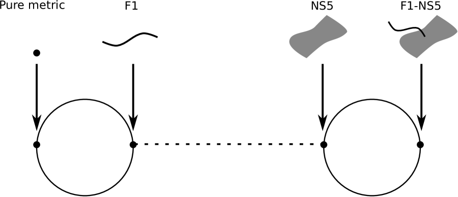
Figure 1: Pictorial representation of the duality chain (4.99). Applying $O(d,d)$ transformations (the left solid circle) to a pure metric, one produces solutions of the ‘F1 type’, then the ‘bridge’ (dashed line) discussed in section 4.2.3 connects the F1 geometry with a pure NS5. Additional $O(d,d)$ transformations, represented by the solid circle on the right, produce the general F1–NS5 solution.

In this article we are studying the symmetries of the NS sector of string theory, and so far we have only discussed the geometries related to pure metric by $O(d,d)$ transformations. Inclusion of S duality allows one to produce more general NS–NS backgrounds, and in this subsection our construction is extended to such geometries.

In the context of black hole physics $O(d,d)$ transformation are often used to generate solutions with electric $B$ field, so we will call them ‘F1 geometries’, even if they do not describe fundamental strings. To generate NS5 branes from black holes one has to use a specific combination of T and S dualities, and we will denote the resulting geometry by ‘NS5’, even though it can contain more general fluxes. This chain of dualities is shown in Figure 1.

To generate the ‘NS5 geometry’ we begin with a ten–dimensional metric reduced on $T^{p}\times T^{4}$:

$$ds_{P}^{2}=H_{\alpha\beta}[dy^{\alpha}+Y^{\alpha}][dy^{\beta}+Y^{\beta}]+G_{ab}(dz^{a}+A^{a})(dz^{b}+A^{b})+h_{mn}dx^{m}dx^{n}$$ (4.98)

To generate a magnetic NS flux, we perform the following dualities [45, 46]:

$$P\stackrel{{\scriptstyle T_{y}}}{{\longrightarrow}}F\stackrel{{\scriptstyle S}}{{\longrightarrow}}D1\stackrel{{\scriptstyle T_{z}}}{{\longrightarrow}}D5\stackrel{{\scriptstyle S}}{{\longrightarrow}}NS5.$$ (4.99)

Notice that various labels just indicate the type of flux (i.e., F1 is an electric $B$–field, D5 is a magnetic $C^{(2)}$ and so on) rather than presence of branes.

T dualities along $y$ directions produces F1 solution, and subsequent S duality gives

$$ds_{D1}^{2} = \sqrt{\mbox{det}\,H}\left[{\tilde{H}}_{\alpha\beta}dy_{\alpha}dy_{\beta}+G_{ab}(dz^{a}+A^{a})(dz^{b}+A^{b})+h_{mn}dx^{m}dx^{n}\right],$$

$$e^{2\Phi} = {\mbox{det}\,H},\quad C^{(2)}=dy_{\alpha}\wedge Y^{\alpha},\quad{\tilde{H}}_{\alpha\beta}=[H^{-1}]_{\alpha\beta}.$$

The outcome of four T dualities along $z$ directions depends on the presence of $z^{a}$ in $Y^{\alpha}$. If $Y^{\alpha}$ has no legs along $z$ directions, then T dualities produce a six–form, which can be dualized back to $C^{(2)}$. Any leg pointing in $z$ direction leads to $C^{(4)}$, and this RR flux can’t be removed by S duality. Thus to end up with NS system we require $Y$ to point only in the non–compact directions. Then T dualities along $z$ directions give

$$ds_{D5}^{2} = \sqrt{\mbox{det}\,H}\left[{\tilde{H}}_{\alpha\beta}dy_{\alpha}dy_{\beta}+h_{mn}dx^{m}dx^{n}\right]+\frac{1}{\sqrt{\mbox{det}\,H}}{\tilde{G}}_{ab}dz_{a}dz_{b},$$

$$e^{2\Phi} = \frac{1}{{\mbox{det}}\,H{\mbox{det}}\,G},\quad C^{(2)}=dy_{\alpha}\wedge Y^{\alpha}\wedge\prod(dz^{a}+A^{a}),\quad B=dz_{a}\wedge A^{a},$$

where ${\tilde{G}}$ is the inverse matrix of $G$. To avoid the RR fields after S duality, we must require $A^{a}=0$, this leads to the final result:

$$ds_{NS5}^{2} = \sqrt{\mbox{det}\,G}\left[\mbox{det}\,H{\tilde{H}}_{\alpha\beta}dy_{\alpha}dy_{\beta}+{\mbox{det}\,H}h_{mn}dx^{m}dx^{n}+{\tilde{G}}_{ab}dz_{a}dz_{b}\right],$$

$$e^{2\Phi} = {{\mbox{det}}\,H{\mbox{det}}\,G},\quad B=dy_{\alpha}\wedge Y^{\alpha}\wedge\prod(dz^{a}+A^{a}).$$ (4.100)

Separation of the Hamilton–Jacobi equation in the geometry (4.98) implies (among other things) the separation of

$$fh^{mn}\partial_{m}S\partial_{n}S,\quad fH^{\alpha\beta},$$ (4.101)

and for the geometry (4.2.3) we need

$$\frac{\tilde{f}}{{\mbox{det}\,H}\sqrt{{\mbox{det}~{}}G}}h^{mn}\partial_{m}S\partial_{n}S,\quad\frac{\tilde{f}}{{{\mbox{det}\,H}\sqrt{{\mbox{det}~{}}G}}}{\tilde{H}}^{\alpha\beta},\qquad\frac{\tilde{f}}{\sqrt{{\mbox{det}~{}}G}}{\tilde{G}}^{ab}$$ (4.102)

to separate for some function ${\tilde{f}}$. Setting

$${\tilde{f}}={f}{{\mbox{det}\,H}}{\sqrt{{\mbox{det}~{}}G}}$$ (4.103)

we must require

$$\partial_{x}\partial_{y}[{f}h^{mn}\partial_{m}S\partial_{n}S]=0,\quad\partial_{x}\partial_{y}[f{\tilde{H}}^{\alpha\beta}]=0,\ \partial_{x}\partial_{y}{\tilde{f}}=0,\ \partial_{x}\partial_{y}[f{{\mbox{det}\,H}}{\tilde{G}}^{ab}]=0.$$ (4.104)

The first condition is automatic, the second one is similar to the requirement for T duality (recall that ${\tilde{H}}=H^{-1}$), and the last two relations are new. As before, the old and the new Killing tensors are expressed as (4.73)

$$K^{MN}=X^{MN}-f_{x}g^{MN},\quad{\tilde{K}}^{MN}={\tilde{X}}^{MN}-{\tilde{f}}_{x}{\tilde{g}}^{MN},$$ (4.105)

although now tildes refer to the NS5 system. Repeating the steps which led to (4.75), we find

$${\tilde{X}}^{\alpha\beta}=\left[fH^{\alpha\beta}\right]_{x},\ {\tilde{X}}^{ab}=\left[f{{\mbox{det}\,H}}{\tilde{G}}^{ab}\right]_{x},\ {\tilde{X}}^{mn}=X^{mn},\quad{\tilde{f}}_{x}=[{f}{{\mbox{det}\,H}}{\sqrt{{\mbox{det}~{}}G}}]_{x}.$$ (4.106)

Equations (4.103), (4.105), (4.106) give the Killing tensor ${\tilde{K}}$ in terms of the the original metric, in particular, we observe that the expression for ${\tilde{K}}$ in terms of $K$ is rather complicated. This reinforces the principle introduced in section 2.2: to study the Killing tensors and their transformations under dualities, it is convenient to begin with finding the eigenvectors and eigenvalues of the tensors since the map (4.106) between $X$ and ${\tilde{X}}$ is relatively simple. Several explicit examples of Killing tensors for F1–NS5 systems are presented in Appendix G.

4.2.4 Conditions on the $B$ field from separation of variables

Equation (4.104) gives the separability condition for the NS5 metric, and now we present the constraints on the $B$ field. In Section 4.2.1 such restrictions were found by requiring separability of the metrics on any $O(d,d)$ orbit which starts from a pure metric, and now we impose the same requirement on the $O(d,d)$ orbit staring from an NS5 solution. We will find that separability of F1–NS5–P geometries is guaranteed by (4.104) and constraints (4.110), (4.112), (4.113) on the Kalb–Ramond field of the original F1 system.

We start with constraints (4.89) and (4.90) derived for the F1 orbit

$$\partial_{y}(fg^{mM})H_{xMb}+\partial_{x}(fg^{mM})H_{yMb}+fg^{mM}\partial_{x}H_{yMb}=0,$$

$$\partial_{x}\partial_{y}(fg_{ab})-fg^{MN}H_{yaM}H_{xNb}-fg^{MN}H_{xaM}H_{yNb}=0,$$ (4.107)

and require them to hold for NS5 solutions as well. Then using the relation between metrics for F1 and NS5 (4.2.3),

$$g_{MN}^{NS5}=Fg_{MN}^{F1},\quad f^{NS5}=Ff^{F1},\quad F\equiv\sqrt{\mbox{det}G}\,\mbox{det}H=e^{-2\Phi_{F1}}$$ (4.108)

and electric–magnetic duality transformation, we can rewrite (4.2.4) in terms of the metric and the $B$ field for F1. The detailed calculations presented in the Appendix E give

$$\partial_{x}\partial_{y}[g_{ab}fF]+\frac{f}{F}g_{ab}\Big{[}\partial_{x}\ln F\partial_{y}\ln F+\frac{1}{2}H_{xMN}H_{y}{}^{MN}\Big{]}=0$$ (4.109)

and

$$\partial_{y}(fg^{mM})H_{xMb}+\partial_{x}(fg^{mM})H_{yMb}+fg^{mM}\partial_{x}H_{yMb}=0,$$ (4.110)

$$\partial_{y}(fg^{mM})\tilde{H}_{xMb}+\partial_{x}(fg^{mM})\tilde{H}_{yMb}+\frac{1}{F}fg^{mM}\partial_{x}(F\tilde{H}_{yMb})=0,$$

where $\tilde{H}=\star_{6}H^{(F1)}$ is the Hodge dual dual of $H^{(F1)}$ with respect to the metric $h_{mn}$.

Interestingly, in all examples we have considered, two terms in equation (4.109) vanish separately, and perhaps such ‘coincidence’ is guaranteed by equations of motion of supergravity for the NS5 brane, but we have not investigated this further. Vanishing of the first term in equation (4.109) implies separation of a very interesting duality–invariant quantity

$$g^{(F1)}_{ab}f^{(F1)}e^{-2\Phi_{F1}}=g^{(NS5)}_{ab}f^{(NS5)}e^{-2\Phi_{NS5}}.$$ (4.111)

Then vanishing of the second term in (4.109) implies a relation in the F1 frame:

$$\partial_{x}\Phi\partial_{y}\Phi+\frac{1}{8}H_{xMN}H_{y}{}^{MN}=0.$$ (4.112)

To summarize, the separability of the F1–NS5–P geometries obtained form the F1 system is guaranteed by equation (4.104), conditions (4.110), (4.112) on the $B$ field of the original F1 system, and

$$\partial_{x}\partial_{y}[g_{ab}fe^{-2\Phi}]=0.$$ (4.113)

4.3 T duality and the modified Killing–Yano equation

In this subsection we investigate the behavior of (conformal) Killing–Yano tensors under T dualities. We will show that generically T duality destroys Killing–Yano tensors, but there is a unique modification of the KYT equation which is invariant under T duality. For the geometries without Kalb–Ramond field, this modified Killing–Yano (mKY) equation reduces to the standard one (2.9), but in general it also contains contributions from the $B$ field. To motivate the mKYT equation, we apply T duality to a pure metric. This leads to the unique modification of KYT equation in the dual frame, and we will demonstrate that such modification remains invariant under any combination of diffeomorphisms and T dualities.

Let us start with a standard equation for the Killing–Yano tensor (2.8)

$$\nabla_{M}Y_{NP}+\nabla_{N}Y_{MP}=0$$ (4.114)

and perform a dimensional reduction of the metric along $z$ direction:

$$ds^{2}=e^{C}[dz+A_{i}dx^{i}]^{2}+\hat{g}_{ij}dx^{i}dx^{j}.$$ (4.115)

In the first step of our analysis we also assume that geometry (4.115) has a trivial Kalb–Ramond field. The details of the reduction are given in Appendix D.2, in particular, the $(mnp)$ component of the KY equation can be read off from (D.2) by setting $L=Y$:

$$\nabla^{m}Y^{np}+{1\over 2}F^{mp}Y^{n}{}_{z}+(m\leftrightarrow n)=0,$$ (4.116)

where $F=dA$ is the field strength associated with graviphoton. We will now look for the modification of the KYT equation in the dual frame that satisfies five requirements:

1. The equation should be linear in the dual Killing-Yano tensor ${\tilde{Y}}$.

2. Its $(mnp)$ component must reproduce (4.116) and other components must be consistent with dimensional reduction of (4.114).

3. The equation must be invariant under gauge transformations of the $B$ field.

4. The new terms to be at most linear in $B$ field since equations (4.116) are linear in $F_{ab}$. This implies that the modified KY equation should be linear in $H_{MNP}$.

5. The square of the modified KYT should give a Killing tensor in the dual frame.

As demonstrated in the in Appendix D.6, there exists a unique modification of equation (4.114) which satisfies all these requirements, and it reads

$$\boxed{{\tilde{\nabla}}_{M}{\tilde{Y}}_{NP}+{\tilde{\nabla}}_{N}{\tilde{Y}}_{MP}+\frac{1}{2}\tilde{H}_{MPA}{\tilde{g}}^{AB}{\tilde{Y}}_{NB}+\frac{1}{2}\tilde{H}_{NPA}{\tilde{g}}^{AB}{\tilde{Y}}_{MB}=0.}$$ (4.117)

Moreover, the Kalb–Ramond field in the dual frame satisfies a constraint

$${{\tilde{H}}_{Q[MN}{\tilde{Y}}_{P]}^{\ \ Q}+\partial_{[P}C\,{\tilde{Y}}_{MN]}=-\partial_{[P}{\tilde{W}}_{MN]}}$$ (4.118)

with some antisymmetric tensor ${\tilde{W}}_{MN}$. Under the T duality the components of the mKYT transform as

$$\tilde{Y}^{mn}=Y^{mn},\quad\tilde{Y}^{n}{}_{z}=e^{-C}Y^{n}{}_{z}.$$ (4.119)

The counterpart of the constraint (4.118) in the original metric (4.115) is

$$dC\wedge dY=0.$$ (4.120)

Notice that (4.117) can be interpreted as a standard KYT equation with connection modified by torsion [47]

$$\Gamma_{MN}^{P}\rightarrow\Gamma_{MN}^{P}-\frac{1}{2}H^{P}{}_{MN}.$$ (4.121)

In Appendix I we discuss transformation of Kähler structure under T duality and demonstrate that a counterpart of the transformation (4.119) maps the Kähler form into complex structure satisfying the Strominger’s system for manifolds with torsion [47].

Although equation (4.117) was derived by applying T duality to a pure metric, the result is invariant under any combination of T dualities and diffeomorphisms. In Appendix D.6 we demonstrate that T duality maps any solution $Y_{MN}$ of (4.117) in an arbitrary geometry (4.115) supported by the $B$ field into a solution ${\tilde{Y}}_{MN}$ of the same equation in the dual frame. The transformation (4.119) between tensors can be viewed as an extension of Buscher’s rules to Killing–Yano tensors. The constraint (4.118) is generalized as

$$g^{ms}\partial_{s}C{\hat{Y}}^{n}{}_{z}-g^{ns}\partial_{s}C{\hat{Y}}^{m}{}_{z}+g^{ns}G_{sr}Y^{rm}-g^{ms}G_{sr}Y^{rn}=0,$$ (4.122)

$$\quad G_{mn}\equiv e^{C/2}F_{mn}-e^{-C/2}{\tilde{F}}_{mn},\quad{\hat{Y}}_{z}{}^{s}\equiv e^{-C/2}Y_{z}{}^{s}\,,$$

where $F_{mn}$ and ${\tilde{F}}_{mn}$ are graviphotons in the original and dual frames. Notice that ${\hat{Y}}_{z}{}^{s}$ remains invariant under T duality, and $G_{mn}$ changes sign.

To summarize, we have demonstrated that the requirement of covariance under T duality leads to the unique equation (4.117) for the KYT, and the original equation (4.114) is transformed into the system (4.117)–(4.118). In other words, unlike the KV and KT equations which are unaffected by the Kalb–Ramond field, the equation for the Killing–Yano tensor is modified, which is not very surprising since fermions interact with the $B$ field. In all three cases (KV, KT, mKYT) the Kalb–Ramond field satisfies additional constraints in the dual frame (see (4.11), (4.96), (4.118)).

Although Ramond–Ramond fluxes appeared in the intermediate stages of the duality chain (4.99), neither the initial nor the final point contained such fields. Unfortunately an extension of our analysis to Ramond–Ramond backgrounds leads to certain complications, which we now discuss. Starting with a pure metric and performing a T duality, we find the new mKYT from (4.119):

$$\tilde{Y}^{mn}=Y^{mn},\quad\tilde{Y}^{n}{}_{z}=e^{-C}Y^{n}{}_{z}.$$ (4.123)

Since the mKYT equation is written in the string frame, S duality induces a conformal rescaling of such metric, so generically the modified Killing–Yano tensor is destroyed by such operation. To save it we have two option for the equation after the duality:

1. Postulate that in the presence of the Ramond–Ramond fluxes, the covariant derivatives appearing in the mKYT should be computed using $g^{\prime}_{MN}=e^{-\Phi}g_{MN}$ rather that $g_{MN}$, and $H_{3}$ should be replaced by $F_{3}$. While consistent with S duality, this prescription does not reduce to the standard KYT in the NS–NS backgrounds with non–trivial dilaton, so it should be abandoned.

2. Postulate that the modified KYT equation survives S duality only if the constraint

   $$g^{AB}\partial_{B}\Phi Y_{AM}=0$$ (4.124)

   is satisfied. Then the discussion presented in the Appendix A.2 implies that the mKYT transforms according to (A.8)

   $$Y^{\prime}_{NP}=e^{-3\Phi/2}{\tilde{Y}}_{NP},$$ (4.125)

   where ${\tilde{Y}}_{NP}$ satisfies equation (4.117) before S duality, and $\Phi$ is the dilaton for the NS system.

Although option (b) is not ruled out, the constraint (4.124) is rather restrictive. Moreover, even assuming that this constraint is satisfied, and equation (4.117) does hold for the type IIB theory with replacement $H_{3}\rightarrow F_{3}$, an additional T duality to type IIA supergravity leads to rather unusual structures. By applying the dimensional reduction and T duality to Ramond–Ramond background, we found that the KY equation in the dual frame mixes tensors of different ranks. For example, starting with mKYT $Y_{MN}$ one produces an equation that mixes $Y^{(1)}_{M}$ and $Y^{(3)}_{MNP}$. This is not surprising since something similar happens for components of $F_{3}$, but KYT become rather complicated. While it would be very interesting to study the properties of such objects with mixed ranks and perhaps embed them in the democratic formalism [48], this direction will not be pursued here.

Finally we comment on behavior of conformal Killing(–Yano) tensors. As demonstrated in section 4.1.3, T duality introduces $z$–dependence in conformal Killing vectors, so such dependence should be allowed in CKT as well. Dimensional reduction for a relatively simple case $A_{m}=0$ is performed in Appendix D.5, where we demonstrate that generically CKTs are destroyed by T duality. However, the CKT does survive the duality if two additional conditions (D.57) and (D.5) are satisfied. The same conclusion holds for a conformal mKYT: it survives T duality only in very special cases.

5 Examples of the modified KYT for F1–NS5 system

In this section we present several examples of the modified Killing–Yano tensors introduced in section 4.3. As we saw in section 3, the ordinary Killing–Yano tensors exist for a large class of black holes described by the Myers–Perry solutions, and these geometries automatically solve our modified equation since they do not have a Kalb–Ramond field. However, string theory provides a very nice generating technique that allows one to start with a known solution of general relativity and construct black holes with various charges by applying string dualities [42, 43, 49]. In this article we are focusing only on the NS–NS sector of string theory, so we will use the special cases of the general techniques introduced in [42, 43, 49] to produce black holes with fundamental string and NS5–brane charges. For such special cases, it is convenient to specify the duality transformations more explicitly.

We will start with a rotating black hole in $d<10$ dimensions and boost it in one of the $10-d$ direction. Then application of T duality along that direction produces a non–extremal fundamental string. To arrive at an NS5–brane (and more generally at a combination of strings and NS5–branes), one has to apply a more sophisticated procedure introduced in [45, 46]:

1. Start with a rotating Myers–Perry black hole with mass $m$ in $d<6$ dimensions, perform a trivial embedding into the ten–dimensional type IIA supergravity, and identify a five–dimensional torus $T^{4}\times S^{1}$ orthogonal to the black hole.

2. Perform a boost by $\alpha$ along $S^{1}$ direction and T–dualize along $S^{1}$. This produces a black fundamental string wrapping one of the compact directions.

3. Perform an S duality followed by four T dualities along $T^{4}$ and another S duality. The resulting metric describes a non–extremal rotating NS5 brane.

4. Perform another boost by $\beta$ in the $S^{1}$ direction followed by T duality. This gives a non–extremal F1–NS5 system with mass $m$ and charges

   $$Q_{1}=m\sinh^{2}\beta,\qquad Q_{5}=m\sinh^{2}\alpha.$$ (5.1)

For future reference we summarize the duality chain using a simple diagram:

$$\mbox{BH}\ \rightarrow\ \mbox{P}_{\alpha}\ \rightarrow\ \mbox{F1}_{\alpha}\ \rightarrow\ \mbox{D1}_{\alpha}\ \rightarrow\ \mbox{D5}_{\alpha}\ \rightarrow\ \mbox{NS5}_{\alpha}\ \rightarrow\ \left(\begin{array}[]{c}\mbox{NS5}_{\alpha}\\ P_{\beta}\end{array}\right)\ \rightarrow\left(\begin{array}[]{c}\mbox{NS5}_{\alpha}\\ F1_{\beta}\end{array}\right).$$ (5.6)

In this section we use $y$ to denote the $S^{1}$ direction. Notice that if we are adding only the F1 charge, the duality chain stops after the first two steps, and four–dimensional torus is not needed. Thus such charge can be added to the Myers–Perry black hole in $d<10$ dimensions, and we derive the explicit expression for the corresponding mKYT in section 5.1. On the other hand, addition of the NS5 charge needs $T^{4}\times S^{1}$, so it only works for black holes with $d<6$. Since we are interested in asymptotically–flat geometries, the BTZ black hole [50] will not appear in the discussion, so $d$ can take only two values ($d=4,5$). These cases are discussed in sections 5.2 and 5.3. Our results are summarized in table 1.

	4D		5D
	extremal	non–extremal	extremal	non-extremal
F1	M	M	M	M
NS5	M	–	M	M
F1–NS5($Q_{1}=Q_{5}$)	–	–	C,M	M
F1–NS5($Q_{1}\neq Q_{5}$)	–	–	M	M

Table 1: Summary of the results for the F1–NS5 system constructed from four– and five–dimensional black holes using the procedure (5.6). Here M denotes the modified KYT and C correspond to the conformal KYT.

5.1 Charged Myers–Perry black hole

In our first example we add charges to the Myers–Perry black hole discussed in section 3 by applying the duality chain (5.6) and discuss the modified Killing–Yano tensor for the resulting solution. The transition from F1 to NS5 in (5.6) involves the electric–magnetic duality, which depends on the dimension of the black hole, so it is convenient to study individual black holes separately, and we will do that in sections 5.2, 5.3. In this section we will focus the first two algebraic steps in the duality chain (5.6) to generate a rotating black hole with F1 charge.

As demonstrated in Appendix F, the charged Myers–Perry black hole admits a family of modified Killing–Yano tensors, which generalizes (3)–(3.31): the tensors are still given by (3.30), (3.31)

$$Y^{(2n-2p)}=\star\left[\wedge h^{p}\right],\quad h=re^{r}\wedge e^{t}+\sum_{k}\sqrt{-x_{k}}e^{x_{k}}\wedge e^{k}\,,$$ (5.7)

but the frames are modified

$$e^{r} = \sqrt{\frac{FR}{R-mr}}dr,\quad e^{x_{i}}=\sqrt{-\frac{(r^{2}-x_{i})d_{i}}{4x_{i}H_{i}}}dx_{i},$$

$$e^{t} = \frac{1}{h_{1}}\sqrt{\frac{R-mr}{FR}}\left[\,\mbox{ch}_{\alpha}dt+\,\mbox{sh}_{\alpha}dy+\sum_{k}\frac{G_{k}}{a_{k}c_{k}^{2}}d\phi_{k}\right],$$

$$e^{y} = \frac{1}{h_{1}}\left[\,\mbox{sh}_{\alpha}dt+\,\mbox{ch}_{\alpha}dy-\frac{mr\,\mbox{sh}_{\alpha}}{FR}dt-\frac{mr\,\mbox{sh}_{\alpha}\,\mbox{ch}_{\alpha}}{FR}\sum_{k}\frac{d\phi_{k}}{a_{k}c_{k}^{2}}\right],$$ (5.8)

$$e^{i} = \frac{1}{h_{1}}\sqrt{\frac{H_{i}}{d_{i}(r^{2}-x_{i})}}\left[\,\mbox{ch}_{\alpha}dt+\,\mbox{sh}_{\alpha}dy+\sum_{k}\frac{G_{k}(r^{2}+a_{k}^{2})}{c_{k}^{2}a_{k}(x_{i}+a_{k}^{2})}\left\{1+\frac{mr\,\mbox{sh}^{2}_{\alpha}(r^{2}-x_{i})}{FR(r^{2}+a_{k}^{2})}\right\}d\phi_{i}\right].$$

The expressions for $c_{i},d_{i},H_{i},G_{i},(FR)$ are still given by (3), and

$$h_{1}=1+\frac{m\,\mbox{sh}_{\alpha}^{2}}{FR}.$$ (5.9)

Expressions for the inverse frames exhibit a clear separation between non–cyclic coordinates $(r,x_{i})$:

$$e_{r} = \sqrt{\frac{R-mr}{FR}}\partial_{r},\quad e_{x_{i}}=\sqrt{-\frac{4x_{i}H_{i}}{d_{i}(r^{2}-x_{i})}}\partial_{x_{i}},\quad e_{y}=\,\mbox{ch}_{\alpha}\partial_{y}-\,\mbox{sh}_{\alpha}\partial_{t},$$

$$e_{t} = -\sqrt{\frac{R^{2}}{FR(R-mr)}}\left[\,\mbox{ch}_{\alpha}\partial_{t}-\frac{\,\mbox{sh}_{\alpha}}{R}(R-mr)\partial_{y}-\sum_{k}\frac{a_{k}}{r^{2}+a_{k}^{2}}\partial_{\phi_{k}}\right],$$ (5.10)

$$e_{i} = -\sqrt{\frac{H_{i}}{d_{i}(r^{2}-x_{i})}}\left[\,\mbox{ch}_{\alpha}\partial_{t}-\,\mbox{sh}_{\alpha}\partial_{y}-\sum_{k}\frac{a_{k}}{x_{i}+a_{k}^{2}}\partial_{\phi_{k}}\right].$$

For the odd dimensions we find

$$e^{r} = \sqrt{\frac{FR}{R-mr^{2}}}dr,\quad e^{x_{i}}=\sqrt{\frac{d_{i}(r^{2}-x_{i})}{4H_{i}}}dx_{i},$$

$$e^{t} = \frac{1}{h_{1}}\sqrt{\frac{R-mr^{2}}{FR}}\left[\,\mbox{ch}_{\alpha}dt+\,\mbox{sh}_{\alpha}dy+\sum_{k}\frac{a_{k}G_{k}}{c_{k}^{2}}d\phi_{k}\right],$$

$$e^{y} = \frac{1}{h_{1}}\left[\,\mbox{sh}_{\alpha}dt+\,\mbox{ch}_{\alpha}dy-\frac{m\,\mbox{sh}_{\alpha}}{FR}dt-\frac{m\,\mbox{sh}_{\alpha}\,\mbox{ch}_{\alpha}}{FR}\sum_{k}\frac{a_{k}d\phi_{k}}{c_{k}^{2}}\right],$$ (5.11)

$$e^{i} = \frac{1}{h_{1}}\sqrt{-\frac{H_{i}}{x_{i}d_{i}(r^{2}-x_{i})}}\left[\,\mbox{ch}_{\alpha}dt+\,\mbox{sh}_{\alpha}dy+\sum_{k}\frac{G_{k}a_{k}(r^{2}+a_{k}^{2})}{c_{k}^{2}(x_{i}+a_{k}^{2})}\left\{1+\frac{m\,\mbox{sh}^{2}_{\alpha}(r^{2}-x_{i})}{FR(r^{2}+a_{k}^{2})}\right\}d\phi_{k}\right],$$

$$e^{\psi} = \frac{1}{h_{1}}\sqrt{\frac{\prod a_{i}^{2}}{r^{2}\prod x_{k}}}\left[\,\mbox{ch}_{\alpha}dt+\,\mbox{sh}_{\alpha}dy+\sum\frac{G_{k}(r^{2}+a_{k}^{2})}{c^{2}_{k}a_{k}}\left\{1-\frac{a^{2}_{k}m\,\mbox{sh}_{\alpha}^{2}}{FR(r^{2}+a_{k}^{2})}\right\}d\phi_{k}\right].$$

and

$$e_{r} = \sqrt{\frac{R-mr^{2}}{FR}}\partial_{r},\quad e_{x_{i}}=\sqrt{\frac{4H_{i}}{d_{i}(r^{2}-x_{i})}}\partial_{x_{i}},\quad e_{y}=\,\mbox{ch}_{\alpha}\partial_{y}-\,\mbox{sh}_{\alpha}\partial_{t},$$

$$e_{t} = -\sqrt{\frac{R^{2}}{FR(R-mr^{2})}}\left[\,\mbox{ch}_{\alpha}\partial_{t}-\frac{\,\mbox{sh}_{\alpha}}{R}(R-mr^{2})\partial_{y}-\sum_{k}\frac{a_{k}}{r^{2}+a_{k}^{2}}\partial_{\phi_{k}}\right],$$ (5.12)

$$e_{i} = -\sqrt{-\frac{H_{i}}{x_{i}d_{i}(r^{2}-x_{i})}}\left[\,\mbox{ch}_{\alpha}\partial_{t}-\,\mbox{sh}_{\alpha}\partial_{y}-\sum_{k}\frac{a_{k}}{x_{i}+a_{k}^{2}}\partial_{\phi_{k}}\right],$$

$$e_{\psi} = -\sqrt{\frac{\prod a_{i}^{2}}{r^{2}\prod x_{k}}}\left[\,\mbox{ch}_{\alpha}\partial_{t}-\,\mbox{sh}_{\alpha}\partial_{y}-\sum_{k}\frac{1}{a_{k}}\partial_{\phi_{k}}\right].$$

The expressions for $c_{i},d_{i},H_{i},G_{i},(FR)$ are still given by (3.36), (3), and $h_{1}$ is given by (5.9).

5.2 F1–NS5 system from the Kerr black hole.

Application of the duality chain (5.6) to the Kerr black hole (2.3) gives a rotating F1–NS5 system, and the complete solution is presented in Appendix G.1 (see equation (G.1)). Explicit calculations show that the modified Killing–Yano equation (4.117) does not have nontrivial solutions, so in this subsection we will focus on two special cases when the mKYT exists: the non–extremal fundamental string and the extremal NS5 brane. In the first case the existence of solution is guaranteed by the general construction presented in section 4.3 as long as condition (4.120) is satisfied, and in the second case the mKYT comes from solving the Killing equations.

Application of the first two steps in the duality sequence (5.6) to Kerr geometry (2.3) leads to the system which we called F1_α, and the corresponding geometry describes a non–extremal fundamental string with charge $Q_{1}=2m\,\mbox{sh}_{\alpha}^{2}$:

$$ds^{2} = \frac{dy^{2}}{h_{\alpha}}+\frac{\rho^{2}}{\Delta}dr^{2}+\rho^{2}d\theta^{2}-\left[\frac{\Delta}{\rho^{2}}+\frac{4(mr\,\mbox{sh}_{\alpha})^{2}}{\rho^{4}h}\right](\,\mbox{ch}_{\alpha}dt-as_{\theta}^{2}d\phi)^{2}$$ (5.13)

$$\qquad+\frac{s_{\theta}^{2}}{\rho^{2}}\left[(r^{2}+a^{2})d\phi-a\,\mbox{ch}_{\alpha}dt\right]^{2}+(\,\mbox{sh}_{\alpha}dt)^{2}$$

$$B_{2} = \frac{2mr\,\mbox{sh}_{\alpha}}{\rho^{2}h}\left[\,\mbox{ch}_{\alpha}dt-as_{\theta}^{2}d\phi\right]\wedge dy,\qquad e^{2\Phi}=\frac{1}{h_{\alpha}}.$$

Here we defined

$$\rho^{2}=r^{2}+a^{2}c^{2}_{\theta},\quad\Delta=r^{2}+a^{2}-2mr,\quad h_{\alpha}=1+\frac{2mr\,\mbox{sh}_{\alpha}^{2}}{\rho^{2}}.$$

Transformation (4.119) leads to the modified Killing–Yano tensor for (5.13)

$$Y = \frac{1}{h_{\alpha}}\left\{rs_{\theta}d\theta\wedge\left[(r^{2}+a^{2})d\phi-a\,\mbox{ch}_{\alpha}dt\right]+ac_{\theta}dr\wedge\left[\,\mbox{ch}_{\alpha}dt-as_{\theta}^{2}d\phi\right]\right\}$$ (5.14)

$$+\frac{\,\mbox{sh}_{\alpha}}{h_{\alpha}}(ac_{\theta}dr-ars_{\theta}d\theta)\wedge dy+\frac{h_{\alpha}-1}{h_{\alpha}}r^{3}s_{\theta}d\theta\wedge d\phi.$$

To compare it with (2.52), we construct the Killing tensor $K_{MN}=-Y_{MA}{Y^{A}}_{N}$, define the frames as eigenvectors of this tensor, and rewrite the answer in terms of them:

$$ds^{2} = -e_{t}^{2}+e_{y}^{2}+e_{r}^{2}+e_{\theta}^{2}+e_{\phi}^{2},$$

$$Y = re_{\theta}\wedge e_{\phi}+ac_{\theta}e_{r}\wedge e_{t},\quad K=r^{2}[e_{\theta}^{2}+e_{\phi}^{2}]+(ac_{\theta})^{2}[e_{t}^{2}-e_{r}^{2}]$$

$$e_{t} = \frac{\sqrt{\Delta}}{\rho h_{\alpha}}\left(\,\mbox{sh}_{\alpha}dy+\,\mbox{ch}_{\alpha}dt-as^{2}_{\theta}d\phi\right),\quad e_{r}=\frac{\rho}{\sqrt{\Delta}}dr,\quad e_{\theta}=\rho d\theta,$$ (5.15)

$$e_{y} = \frac{1}{h_{\alpha}}\left[\,\mbox{ch}_{\alpha}dy+\,\mbox{sh}_{\alpha}\left(1-\frac{2mr}{\rho^{2}}\right)dt+\frac{amrs^{2}_{\theta}\,\mbox{sh}_{2\alpha}}{\rho^{2}}d\phi\right],$$

$$e_{\phi} = \frac{s_{\theta}}{\rho h_{\alpha}}\left(-a\,\mbox{sh}_{\alpha}dy-a\,\mbox{ch}_{\alpha}dt+(r^{2}+a^{2}+2mr\,\mbox{sh}^{2}_{\alpha})d\phi\right).$$

Notice that eigenvalues of the Killing tensor and mKYT do not depend on the boost parameter $\alpha$.

The duality sequence (5.6) involves D-branes supported by Ramond–Ramond flux, and the analysis presented in section 4.3 does not apply to T duality performed in such systems. It would be interesting to generalize our discussion of mKYT to the geometries with Ramond–Ramond fields, but such analysis goes beyond the scope of this article. Instead we applied the duality chain (5.6) to the Kerr black hole and solved the mKYT equations for the resulting F1–NS5 geometry. We found that the mKYT does not exist in the system involving NS5 branes unless one takes an extremal limit and sets the F1 charge to zero:

$$m\rightarrow 0,\ Q_{1}\rightarrow 0,\quad\mbox{fixed}\quad Q_{5}=2m\sinh^{2}\alpha.$$ (5.16)

The resulting geometry,

$$ds^{2} = -dt^{2}+h\left[\frac{\rho^{2}}{r^{2}+a^{2}}dr^{2}+\rho^{2}d\theta^{2}+(r^{2}+a^{2})s_{\theta}^{2}d\phi^{2}+dy^{2}\right],$$

$$B_{2} = \frac{Q_{5}(r^{2}+a^{2})c_{\theta}}{\rho^{2}}d\phi\wedge dy,\quad e^{2\Phi}=h,\quad h=1+\frac{Q_{5}r}{r^{2}+a^{2}},$$ (5.17)

admits the unique mKYT

$$Y = hdy\wedge(rs_{\theta}d\theta-c_{\theta}dr)+hd\phi\wedge[rs_{\theta}^{2}dr+(r^{2}+a^{2})s_{\theta}c_{\theta}d\theta]$$ (5.18)

$$= hd\left[rc_{\theta}dy-\frac{1}{2}(r^{2}+a^{2})s_{\theta}^{2}d\phi\right]$$

which was found by the direct calculation. Introducing convenient frames, we can rewrite this KYT and its square as

$$Y = e_{r}\wedge e_{y}-e_{\theta}\wedge e_{\phi},\qquad K\equiv-Y_{MA}Y^{A}{}_{N}dx^{M}dx^{N}=e_{r}^{2}+e_{y}^{2}+e^{2}_{\theta}+e^{2}_{\phi},$$

$$e_{t} = dt,\quad e_{r}=\sqrt{\frac{\rho^{2}+Qr}{r^{2}+a^{2}}}dr,\quad e_{\theta}=\sqrt{\rho^{2}+Qr},$$ (5.19)

$$e_{y} = \frac{1}{\rho^{2}}\sqrt{(r^{2}+a^{2})(\rho^{2}+Qr)}\left[\cos\theta dy+r\sin^{2}\theta d\phi\right],$$

$$e_{\phi} = \frac{\sin\theta}{\rho^{2}}\sqrt{(\rho^{2}+Qr)}\left[rdy-(r^{2}+a^{2})\cos\theta d\phi\right].$$

Notice that square of the KYT gives the spacial part of the metric, which can be viewed as a linear combination of two ‘trivial’ Killing tensors: one coming form the metric and one built from the square of the Killing vector $\partial_{t}$.

An additional T duality along $y$ direction in (5.2) produces a metric of the extremal KK monopole, and application of (4.119) to (5.18) gives the standard KYT for the monopole:

$$Y=dr\wedge[(Q+r\sin^{2}\theta)d\phi+\cos\theta dy]+d\theta\wedge[\cos\theta\sin\theta(a^{2}+r^{2})d\phi-r\sin\theta dy].$$ (5.20)

In the frames we find

$$Y = e_{r}\wedge e_{y}-e_{\theta}\wedge e_{\phi},\qquad K=e_{r}^{2}+e_{y}^{2}+e^{2}_{\theta}+e^{2}_{\phi},$$

$$e_{t} = dt,\quad e_{r}=\sqrt{\frac{\rho^{2}+Qr}{r^{2}+a^{2}}}dr,\quad e_{\theta}=\sqrt{\rho^{2}+Qr},$$

$$e_{y} = \sqrt{\frac{r^{2}+a^{2}}{\rho^{2}+Qr}}\left[\cos\theta dy+(Q+r\sin^{2}\theta)d\phi\right],$$ (5.21)

$$e_{\phi} = \frac{\sin\theta}{\sqrt{\rho^{2}+Qr}}\left[rdy-\cos\theta(r^{2}+a^{2})d\phi\right].$$

Once again, the KYT squares to a ‘trivial” Killing tensor.

5.3 F1–NS5 system from the five–dimensional black hole.

Application of the duality chain (5.6) to the five–dimensional black hole gives another example of the rotating F1–NS5 system, the complete geometry was found in [49, 51], and it is given by equation (G.2). This subsection discusses the modified Killing–Yano tensor for this solution.

Recalling that even the neutral five–dimensional black hole had the KYT of rank three rather than two (see section 2.3), we should look at the obvious extension of (4.117) to such objects:

$${\nabla}_{M}{Y}_{NPQ}+{\nabla}_{N}{Y}_{MPQ}+\frac{1}{2}H_{MPA}{g}^{AB}{Y}_{NBQ}+\frac{1}{2}H_{MQA}{g}^{AB}{Y}_{NPB}$$

$$+\frac{1}{2}H_{NPA}{g}^{AB}{Y}_{MBQ}+\frac{1}{2}H_{NQA}{g}^{AB}{Y}_{MPB}=0.$$ (5.22)

The general construction of section 4.3 guarantees existence of the mKYT for $\alpha=0$ (as long as constraint (4.120) is satisfied), but the generation of the NS5 branes goes through Ramond–Ramond fluxes, which can potentially destroy the modified KYT. Remarkably, the tensor survives, and solution of (5.3) for the geometry (G.2) is

$$Z^{-1}Y = -ad[r^{2}\cos^{2}\theta]dtd\psi-a\mu_{A}\mu_{B}d[(r^{2}+a^{2}-M)\sin^{2}\theta]d\phi dy$$

$$+a\mu_{A}d[(r^{2}+a^{2}-M)\sin^{2}\theta]dtd\phi-a\mu_{B}d[r^{2}\cos^{2}\theta]dyd\psi+\sigma d[\sin^{2}\theta]d\phi d\psi$$

with

$$Z = \frac{r^{2}+A^{2}+a^{2}c_{\theta}^{2}}{r^{2}+B^{2}+a^{2}c_{\theta}^{2}},\quad\sigma=\frac{(a^{2}-M)A^{2}B^{2}-[a^{2}+A^{2}+B^{2}]Mr^{2}-Mr^{4}}{\sqrt{A^{2}+M}\sqrt{B^{2}+M}},$$

$$\mu_{A} = \frac{A}{\sqrt{M+A^{2}}},\quad\mu_{B}=\frac{B}{\sqrt{M+B^{2}}},\quad s_{\theta}=\sin\theta,\quad c_{\theta}=\cos\theta,$$ (5.24)

$$A = \sqrt{M}\sinh\alpha,\qquad B=\sqrt{M}\sinh\beta.$$

Although expression (5.3) is already relatively simple, we also rewrite it in frames to connect to the general analysis presented in section 2.3. Constructing the Killing tensor $K_{MN}=-Y_{MA}{Y^{A}}_{N}$ and defining the frames as its eigenvectors, we find

$$ds^{2} = -e_{t}^{2}+e_{y}^{2}+e_{r}^{2}+e_{\theta}^{2}+e_{\phi}^{2}+e_{\psi}^{2},$$

$$Y = \left(a\sqrt{2A^{2}+2Mc^{2}_{\theta}}\,e_{r}\wedge e_{t}+\sqrt{2M(A^{2}+r^{2})-2a^{2}A^{2}}e_{\theta}\wedge e_{\phi}\right)\wedge e_{\psi},$$

$$K = -\frac{1}{2}Y_{MA}{Y^{A}}_{N}=[M(A^{2}+r^{2})-a^{2}A^{2}][e^{2}_{\theta}+e^{2}_{\phi}]+a^{2}(A^{2}+Mc_{\theta}^{2})[e^{2}_{t}-e^{2}_{r}]$$ (5.25)

$$+[a^{2}(A^{2}+Mc_{\theta}^{2})-(M(A^{2}+r^{2})-a^{2}A^{2})]e_{\psi}^{2},$$

where the frames are given by

$$e_{t} = \frac{r}{\rho^{2}H_{1}}\sqrt{\frac{M\Delta\rho^{2}H_{5}}{M(A^{2}+r^{2})-a^{2}A^{2}}}\left[\,\mbox{ch}_{\beta}dt+\,\mbox{sh}_{\beta}dy-a(\,\mbox{sh}_{\alpha}c_{\theta}^{2}d\psi-\,\mbox{ch}_{\alpha}s_{\theta}^{2}d\phi)\right],$$

$$e_{y} = \frac{1}{2\rho^{2}H_{1}}\Bigg{[}2\,\mbox{sh}_{\beta}\left(\rho^{2}-M\right)dt+2\rho^{2}\,\mbox{ch}_{\beta}dy+aM\,\mbox{sh}_{2\beta}(\,\mbox{sh}_{\alpha}c_{\theta}^{2}d\psi-\,\mbox{ch}_{\alpha}s_{\theta}^{2}d\phi)\Bigg{]},$$

$$e_{r} = \sqrt{\frac{A^{2}+\rho^{2}}{\Delta}}dr,\quad e_{\theta}=\sqrt{A^{2}+\rho^{2}}d\theta,$$ (5.26)

$$e_{\phi} = \frac{s_{\theta}c_{\theta}}{\rho H_{1}}\sqrt{\frac{MH_{5}}{A^{2}+Mc^{2}_{\theta}}}\Bigg{[}a\,\mbox{ch}_{\beta}dt+a\,\mbox{sh}_{\beta}dy+(B^{2}+r^{2})(\,\mbox{sh}_{\alpha}d\psi+\,\mbox{ch}_{\alpha}d\phi)+a^{2}\,\mbox{ch}_{\alpha}d\phi\Bigg{]},$$

$$e_{\psi} = \frac{1}{\rho^{2}H_{1}\sqrt{A^{2}+Mc^{2}_{\theta}}\sqrt{M(A^{2}+r^{2})-a^{2}A^{2}}}\Bigg{[}$$

$$[r^{2}+(a^{2}-M)c_{\theta}^{2}]\left(\frac{1}{2}aM\,\mbox{sh}_{2\alpha}(\,\mbox{ch}_{\beta}dt+\,\mbox{sh}_{\beta}dy)+Ma^{2}\,\mbox{sh}_{\alpha}s_{\theta}^{2}d\phi\right)$$

$$+\left[M(r^{2}+A^{2})(r^{2}+B^{2})+MA^{2}c_{\theta}^{2}r^{2}-A^{2}B^{2}a^{2}\right](\,\mbox{sh}_{\alpha}s_{\theta}^{2}d\phi-\,\mbox{ch}_{\alpha}c_{\theta}^{2}d\psi)\Bigg{]}.$$

For $\alpha=0$ we find

$$e_{t} = \frac{1}{\rho^{2}H_{1}}\sqrt{{\Delta\rho^{2}}}\left[\,\mbox{ch}_{\beta}dt+\,\mbox{sh}_{\beta}dy+as_{\theta}^{2}d\phi\right],$$

$$e_{y} = \frac{1}{2\rho^{2}H_{1}}\Bigg{[}2\,\mbox{sh}_{\beta}\left(\rho^{2}-M\right)dt+2\rho^{2}\,\mbox{ch}_{\beta}dy-aM\,\mbox{sh}_{2\beta}s_{\theta}^{2}d\phi\Bigg{]},$$

$$e_{r} = \sqrt{\frac{\rho^{2}}{\Delta}}dr,\quad e_{\theta}=\sqrt{\rho^{2}}d\theta,\quad e_{\psi}=r\cos\theta d\psi,$$ (5.27)

$$e_{\phi} = \frac{s_{\theta}}{\rho H_{1}}\Bigg{(}a\,\mbox{ch}_{\beta}dt+a\,\mbox{sh}_{\beta}dy+(a^{2}+M\,\mbox{sh}^{2}_{\beta}+r^{2})d\phi\Bigg{)}.$$

This is the special case of (5.1) for $n=1$ and one rotation parameter. Finally we give the expression for the mKYT (5.3) in the extremal limit ($M=0$ with fixed $A,B$):

$$Z^{-1}Y = -\frac{1}{2}d\left[(dt+dy)\left\{(r^{2}c_{\theta}^{2})d\psi-(r^{2}+a^{2})s_{\theta}^{2}d\phi\right\}+ABa\cos^{2}\theta d\phi d\psi\right].$$ (5.28)

5.4 Conformal Killing–Yano tensors

We conclude this section with discussing the CKYT for rotating F1–NS5 systems. Explicit calculations show that the geometry obtained by application of (5.6) to the Kerr solution (2.3) does not have CKYT. On the other hand F1–NS5 system constructed from the five–dimensional black hole (2.3) does admit a CKYT if and only if $Q_{1}=Q_{5}$. In this case the metric has the form

$$ds^{2} = -e_{t}^{2}+e_{\phi}^{2}+e_{y}^{2}+e_{\psi}^{2}+e_{r}^{2}+e_{\theta}^{2},$$

$$e_{t} = \frac{\sqrt{\Delta}}{\rho}(dt-as_{\theta}^{2}d\phi),\quad e_{\phi}=\frac{s_{\theta}}{\rho}\left[(r^{2}+a^{2}+Q)d\phi-adt\right],$$ (5.29)

$$e_{r} = \frac{\rho}{\sqrt{\Delta}}dr,\quad e_{\bf\theta}=\rho d\theta,\quad e_{\psi}=\frac{c_{\theta}}{\rho}[(Q+r^{2})d\psi-ady],\quad e_{y}=\frac{r}{\rho}[dy+ac_{\theta}^{2}d\psi],$$

$$\Delta = r^{2}+a^{2}-M,\quad\rho^{2}=r^{2}+a^{2}c_{\theta}^{2}+Q,$$

and the corresponding CKYT and CKT are given by

$${\cal Y} = \rho(e_{r}\wedge e_{t}\wedge e_{y}+e_{\theta}\wedge e_{\phi}\wedge e_{\psi}),\quad Z=\frac{1}{\rho^{2}}(ac_{\theta}e_{\psi}-re_{y})\wedge(\sqrt{\Delta}e_{t}+as_{\theta}e_{\phi}),$$

$${\cal K} = \rho^{2}[e_{t}^{2}-e_{r}^{2}-e_{y}^{2}+e_{\theta}^{2}+e_{\psi}^{2}+e_{\phi}^{2}],\quad W=-d[r^{2}-a^{2}c_{\theta}^{2}].$$ (5.30)

Since $W$ is a total derivative, the general prescription (2.18) can be used to construct a standard Killing tensor

$$K=-[2(ac_{\theta})^{2}+Q][-e_{t}^{2}+e_{r}^{2}+e_{y}^{2}]+[2r^{2}+Q][e_{\theta}^{2}+e_{\psi}^{2}+e_{\phi}^{2}].$$ (5.31)

Conformal Killing tensors for four– and five–dimensional black holes discussed in this section were constructed in [52] via separation of variables.

6 Discussion

In this article we analyzed hidden symmetries of stringy geometries and their behavior under string dualities. In particular, we demonstrated that in the presence of the Kalb–Ramond field the equation for the Killing–Yano tensor is modified as (4.117), and this is the unique modification consistent with string dualities. The transformations laws for the Killing vectors, tensors, and Killing–Yano tensors are given by (4.1.1), (4.73)–(4.75), (4.119). We have also demonstrated that nontrivial Killing tensors in arbitrary number of dimensions are always associated with ellipsoidal coordinates, and we used this observation to construct the (modified) Killing(–Yano) tensors for the Myers–Perry black hole ((3), (3.30), (3.31)), its charged version (5.7)–(5.1), and for several examples of F1–NS5 geometries ((5.2), (5.3)–(5.3)).

This work has several implications. First and foremost, the modified equation for the Killing–Yano tensor (4.117) provides a new powerful tool for studying symmetries of stringy geometries, which can extend the successful applications of the standard Killing–Yano tensors to physics of black holes [52, 53]. Also, the understanding of hidden symmetries developed in this article can be used to extend the ‘no-go theorems’ for integrability [11] to backgrounds without supersymmetry. Finally, the explicit Killing–Yano tensors for the Myers–Perry black hole and its charged version constructed in sections 3 and 5.1 generalize most of the previously known examples and provide the largest known class of KYT.

Appendix A Conformal transformations of Killing tensors

In this appendix we analyze the behavior of Killing vectors and tensors under conformal rescaling of the metric. In the context of string theory such rescalings appear when one goes from the string to the Einstein frame or when one compares the string frames before and after S duality. In this appendix we will find the restrictions on the dilaton which guarantee that Killing vectors and tensors survive after S duality. We study general conformal Killing vectors and tensors, and reduction to the standard objects is obtained by setting the conformal factors to zero.

A.1 Killing vectors

We begin with considering an equation for the conformal Killing vector (CKV):

$$\nabla_{M}V_{N}+\nabla_{N}V_{M}=2g_{MN}v$$ (A.1)

and writing its counterpart in the rescaled metric:

$$g^{\prime}_{MN}=e^{C}g_{MN}:\qquad\nabla^{\prime}_{M}V^{\prime}_{N}+\nabla^{\prime}_{N}V^{\prime}_{M}=2g^{\prime}_{MN}v^{\prime}.$$ (A.2)

Recalling the transformation of the connections,

$$(\Gamma^{M}_{NP})^{\prime}=\Gamma^{M}_{NP}+\frac{1}{2}\left[\delta^{M}_{P}\partial_{N}C+\delta^{M}_{N}\partial_{P}C-g_{NP}g^{MA}\partial_{A}C\right].$$ (A.3)

we can rewrite the equation for $V^{\prime}$ in terms of the original covariant derivatives:

$$\nabla_{M}(e^{-C}V^{\prime}_{N})+\nabla_{N}(e^{-C}V^{\prime}_{M})=2g_{MN}(v^{\prime}+\frac{1}{2}V^{\prime A}\partial_{A}e^{-C}).$$ (A.4)

Comparing this to (A.1), we find the transformation law for the CKV:

$$V^{\prime}_{M} = e^{C}V_{M}\quad\Rightarrow\quad V^{\prime M}=g^{\prime MN}V^{\prime}_{N}=V^{M},$$

$$v^{\prime} = v-\frac{1}{2}V^{A}\partial_{A}e^{-C}.$$ (A.5)

This implies that CKV always survives the conformal rescaling, but the KV (which must have $v=0$) disappears unless

$$V^{A}\partial_{A}e^{-C}=0.$$ (A.6)

In the context of S duality and transition between string and Einstein frames, the last condition implies that Lie derivatives of the dilaton along the Killing vector must vanish, which is a very natural requirement.

A.2 Killing(–Yano) tensors

Next we look at transformation properties of the conformal Killing–Yano tensor, which satisfies equation

$$\nabla_{M}Y_{NP}+\nabla_{N}Y_{MP}=2g_{MN}W_{P}-g_{MP}W_{N}-g_{NP}W_{M}.$$ (A.7)

Using (A.3) we can rewrite the left hand side of (A.7) in the rescaled frame as

$$\nabla^{\prime}_{M}Y^{\prime}_{NP}+\nabla^{\prime}_{N}Y^{\prime}_{MP}=\nabla_{M}Y^{\prime}_{NP}-\frac{1}{2}\left[\partial_{M}CY^{\prime}_{NP}+\partial_{N}CY^{\prime}_{MP}-g_{MN}g^{AB}\partial_{B}CY^{\prime}_{AP}\right]$$

$$\qquad-\frac{1}{2}\left[\partial_{M}CY^{\prime}_{NP}+\partial_{P}CY^{\prime}_{NM}-g_{MP}g^{AB}\partial_{B}CY^{\prime}_{NA}\right]+(M\leftrightarrow N)$$

$$=\nabla_{M}Y^{\prime}_{NP}-\frac{3}{2}\partial_{M}CY^{\prime}_{NP}+\frac{1}{2}g_{MN}g^{AB}\partial_{B}CY^{\prime}_{AP}+\frac{1}{2}g_{MP}g^{AB}\partial_{B}CY^{\prime}_{NA}+(M\leftrightarrow N)$$

and the full equation becomes

$$e^{3C/2}\nabla_{M}(e^{-3C/2}Y^{\prime}_{NP})+e^{3C/2}\nabla_{N}(e^{-3/2C}Y^{\prime}_{MP})$$

$$\qquad=2g_{MN}(W^{\prime}_{P}e^{C}-\frac{1}{2}g^{AB}\partial_{B}CY^{\prime}_{AP})-\left[g_{MP}(W^{\prime}_{N}e^{C}-\frac{1}{2}g^{AB}\partial_{B}CY^{\prime}_{AN})+(M\leftrightarrow N)\right].$$

To recover the original equation (A.7), we must set

$$Y^{\prime}_{NP}=e^{3C/2}Y_{NP},\quad W^{\prime}_{M}=e^{C/2}(W_{M}+\frac{1}{2}g^{AB}\partial_{B}CY_{AM}).$$ (A.8)

The conformal Killing–Yano tensors of higher rank can be analyzed in a similar fashion, and for the rank $k$ tensor we find

$$Y^{\prime}_{M_{1}\dots M_{k}} = e^{(k+1)C/2}Y_{M_{1}\dots M_{k}},$$ (A.9)

$$W^{\prime}_{M_{2}\dots M_{k}} = e^{(k-1)C/2}W_{M_{2}\dots M_{k}}+\frac{e^{(3k-5)C/2}}{2}g^{AB}\partial_{B}CY_{A{M_{2}\dots M_{k}}}$$

The same calculations show that for Killing tensors we have

$$K^{\prime}_{MN}=e^{2C}K_{MN},\quad W^{\prime}_{M}=e^{C}(W_{M}+g^{AB}\partial_{B}CK_{AM}).$$ (A.10)

Equations (A.9) and (A.10) summarize the behavior of Killing(–Yano) tensors under conformal rescalings.

Appendix B Killing tensors and ellipsoidal coordinates

In this appendix we will justify the procedure for extracting separation of variables from a nontrivial Killing tensor and review an example of ellipsoidal coordinates and their degeneration.

B.1 Ellipsoidal coordinates from Killing tensors

As discussed in section 2.2, existence of a non–trivial Killing tensor leads to separation of variables, and in this appendix we will provide some details of the procedure for extracting the relevant coordinates and the separation function.

We will focus on studying the reduced metric (4), and to simplify the notation we will drop the subscript $red$. Assuming that non–cyclic coordinates separate, we find

$$ds^{2}=\sum g_{k}dx_{k}^{2},\quad K=\sum\Lambda_{k}g_{k}dx_{k}^{2}$$ (B.1)

where $g_{k}$ and $\Lambda_{k}$ are functions of all coordinates. Equations for the Killing tensor give

$$\partial_{i}\Lambda_{i}=0,\quad\partial_{j}\ln g_{i}=\partial_{j}\ln(\Lambda_{i}-\Lambda_{j}),\quad j\neq i$$ (B.2)

and there are no summations in these relations. We will now make an additional assumption of separability:

$$\partial_{j}\partial_{k}\ln g_{m}=0\quad\mbox{for different}\quad(i,j,k).$$ (B.3)

and determine the form of $g_{k}$ and $\Lambda_{k}$. The procedure involves several steps:

1. Equation (B.3) leads to factorization of $g_{1}$

   $$g_{1}=\prod f_{1j}(x_{1},x_{j}),\quad\partial_{j}\ln f_{1j}(x_{1},x_{j})=\partial_{j}\ln(\Lambda_{1}-\Lambda_{j})$$ (B.4)

   which implies factorization of

   $$\Lambda_{1}-\Lambda_{2}=f_{12}(x_{1},x_{2})g_{12}(x_{1},x_{3}\dots).$$ (B.5)

   The same expression can also be obtained by starting with $g_{2}$, but this leads to a different factorization:

   $$\Lambda_{1}-\Lambda_{2}=f_{21}(x_{2},x_{1})g_{21}(x_{2},x_{3}\dots).$$ (B.6)

   Applying $\partial_{1}\partial_{3}$ to the logs of (B.5), (B.6), we conclude that $x_{1}$ dependence factorizes in $g_{12}$. Absorbing the $x_{1}$–dependent factor in $f_{12}(x_{1},x_{2})$, we find

   $$\Lambda_{1}-\Lambda_{2}=f_{12}(x_{1},x_{2})g_{12}(x_{3}\dots).$$

   The left–hand side of the last relation is killed by $\partial_{1}\partial_{2}$ (recall the first relation in (B.2)), so

   $$f_{12}(x_{1},x_{2})=f_{12}^{(1)}(x_{1})-f_{12}^{(2)}(x_{2}).$$ (B.7)

   Repeating the same steps for $x_{3},\dots,x_{n}$, we conclude that

   $$g_{1}=h_{1}(x_{1})\prod_{j}[f_{1j}^{(1)}(x_{1})-f_{1j}^{(j)}(x_{j})],$$

   $$\Lambda_{1}-\Lambda_{j}=[f_{1j}^{(1)}(x_{1})-f_{1j}^{(j)}(x_{j})]g_{1j}(x_{3}\dots x_{n}),\quad\partial_{j}g_{1j}=0.$$ (B.8)

   Since coordinate $x_{1}$ is not special, the last equation can be generalized:

   $$\Lambda_{k}-\Lambda_{j}=[f_{kj}^{(k)}(x_{k})-f_{kj}^{(j)}(x_{j})]g_{kj}(x_{1}\dots x_{n}),\quad\partial_{j}g_{kj}=\partial_{k}g_{kj}=0.$$ (B.9)

2. Assuming that $f_{1j}^{(j)}(x_{j})$ are nontrivial functions of their arguments, we can define new coordinates by setting

   $${\tilde{x}}_{j}\equiv f_{1j}^{(j)}(x_{j}),\quad j>1.$$ (B.10)

   and dropping the tildes. We still have the freedom of making a linear transformation of $x_{k}$, which will be fixed later. Taking a second derivative of (1) with respect to $x_{j}$,

   $$\partial^{2}_{j}\Lambda_{1}=\partial^{2}_{j}\Lambda_{j}+\partial^{2}_{j}\Big{(}[f_{1j}^{(1)}(x_{1})-x_{j}]g_{1j}(x_{2}\dots x_{n})\Big{)}=0.$$

   we conclude that $\Lambda_{1}$ is a linear polynomial in every coordinate $(x_{2},\dots x_{n})$. Furthermore, since $\partial_{2}\Lambda_{2}=0$ we find

   $$\Lambda_{2}=\Lambda_{1}-[f_{12}^{(1)}(x_{1})-x_{2}]g_{12}(x_{3},\dots,x_{n})=\Lambda_{1}+[f_{12}^{(1)}(x_{1})-x_{2}]\partial_{2}\Lambda_{1}$$

   and similarly

   $$\Lambda_{j}=\Lambda_{1}+[f_{1j}^{(1)}(x_{1})-x_{j}]\partial_{j}\Lambda_{1}.$$ (B.11)

3. Next we look at

   $$\Lambda_{2}-\Lambda_{3}=(f_{12}^{(1)}(x_{1})-x_{2})\partial_{2}\Lambda_{1}-(f_{13}^{(1)}(x_{1})-x_{3})\partial_{3}\Lambda_{1}$$

   $$\quad=[f_{12}^{(1)}\partial_{2}\Lambda_{1}-f_{13}^{(1)}\partial_{3}\Lambda_{1}]_{0}+x_{3}[f_{12}^{(1)}\partial_{2}\partial_{3}\Lambda_{1}+\partial_{3}\Lambda_{1}]_{0}-x_{2}[f_{13}^{(1)}\partial_{2}\partial_{3}\Lambda_{1}+\partial_{2}\Lambda_{1}]_{0}$$

   Expressions in the square brackets are evaluated at $x_{2}=x_{3}=0$. Equation (B.9) implies that $(x_{2},x_{3})$ dependence in the last equation must factorize, and this is possible only if

   $$f_{13}^{(1)}(x_{1})=c_{32}f_{12}^{(1)}(x_{1})+d_{32},\quad[f_{12}^{(1)}\partial_{2}\Lambda_{1}-f_{13}^{(1)}\partial_{3}\Lambda_{1}]_{0}=e_{32}$$ (B.12)

   with constant $(c_{32},d_{32},e_{32})$. Similar arguments demonstrate that all $f_{1j}(x_{1})$ are linear polynomials in $f_{12}^{(1)}(x_{1})$, so by re-defining this coordinate,

   $$x_{1}\rightarrow f_{12}^{(1)}(x_{1}),$$

   we conclude that all $f_{1j}(x_{1})$ are linear functions of their arguments. For example,

   $$f_{13}^{(1)}(x_{1})-x_{3}=c_{32}x_{1}+d_{32}-x_{3},$$

   so by making a linear transformation of $x_{3}$, we can simplify the last expression:

   $$f_{13}^{(1)}(x_{1})-x_{3}\rightarrow c_{32}(x_{1}-x_{3}).$$

   Repeating this for $(x_{4}\dots x_{n})$, we find

   $$g_{1}=h_{1}(x_{1})\prod_{j}[x_{1}-x_{j}],\qquad\Lambda_{j}=\Lambda_{1}+[x_{1}-x_{j}]\partial_{j}\Lambda_{1}.$$ (B.13)

4. We will now demonstrate that polynomial $\Lambda_{1}(x_{2},\dots,x_{n})$ must be symmetric under interchange of any pair of its arguments. Without the loss of generality, we focus on $x_{2}$ and $x_{3}$ and write $\Lambda_{1}$ as

   $$\Lambda_{1}=P_{1}x_{2}x_{3}+P_{2}x_{2}+P_{3}x_{3}+P_{4},$$ (B.14)

   where $P_{k}$ are polynomials in $(x_{4}\dots x_{n})$. The second equation in (B.12) gives

   $$e_{32}=x_{1}[\partial_{2}\Lambda_{1}-\partial_{3}\Lambda_{1}]_{0}=x_{1}[P_{2}-P_{3}].$$ (B.15)

   Consistency of this relation requires $P_{2}=P_{3}$, i.e., symmetry of $\Lambda_{1}$ under the interchange of $x_{2}$ and $x_{3}$.

5. Once we established that $\Lambda_{1}(x_{2}\dots x_{n})$ is symmetric, it is convenient to introduce a “generating” linear polynomial $\Lambda(x_{1}\dots x_{n})$ symmetric in its arguments and define

   $$\Lambda_{1}=\partial_{1}\Lambda.$$ (B.16)

   Then the second relation in (B.13) implies

   $$\Lambda_{j}=\partial_{1}\Lambda+(x_{1}-x_{j})\partial_{1}\partial_{j}\Lambda=\partial_{1}\Lambda|_{x_{j}=0}+x_{1}\partial_{1}\partial_{j}\Lambda=\partial_{j}\Lambda|_{x_{1}=0}+x_{1}\partial_{1}\partial_{j}\Lambda=\partial_{j}\Lambda.$$

To summarize, we have demonstrated that in the generic case existence of the Killing tensor in the non–cyclic part of the metric (B.1) implies that

$$g_{k}=h_{1}(x_{k})\prod_{j\neq k}[x_{k}-x_{j}],\qquad\Lambda_{j}=\partial_{j}\Lambda,$$ (B.17)

where $\Lambda(x_{1}\dots x_{n})$ is a linear polynomial in every $(x_{1}\dots x_{n})$ symmetric under interchange of every pair of arguments. This completes the justification of (4)–(2.47), which summarize the extraction of the separable coordinates from a Killing tensor.

B.2 Ellipsoidal coordinates in flat space

In section 2.2 we demonstrated that separation of non–cyclic coordinates generically leads to ellipsoidal coordinates. Our derivation was based on the assumption of generality: we postulated that metric components have non–trivial dependence on all non–cyclic coordinates. If this assumption is dropped, one recovers degenerate cases of ellipsoidal coordinates, and in this appendix we will illustrate this using a well-known example of flat three–dimensional space. Degeneration in higher dimensions is very similar, but its detailed discussion is beyond the scope of this article.

Consider a flat three–dimensional space with a metric

$$ds^{2}=dr_{1}^{2}+dr_{2}^{2}+dr_{3}^{2}.$$ (B.18)

The ellipsoidal coordinates $(x_{0},x_{1},x_{2})$ are defined as three solutions of a cubic equation for $x$ [29]:

$$\frac{r_{1}^{2}}{x-a}+\frac{r_{2}^{2}}{x-b}+\frac{r_{3}^{2}}{x-c}=1,$$ (B.19)

Without the loss of generality we assume that non–degenerate coordinates have $a>b>c$ and the roots are arranged in the following order:

$$x_{0}>a>x_{1}>b>x_{2}>c.$$ (B.20)

Cartesian coordinates $(r_{1},r_{2},r_{3})$ can be expressed in terms of $(x_{0},x_{1},x_{2})$ as

$$r_{1}=\left[\frac{(x_{0}-a)(x_{1}-a)(x_{2}-a)}{(a-b)(a-c)}\right]^{1/2},\quad r_{2}=\left[\frac{(x_{0}-b)(x_{1}-b)(x_{2}-b)}{(b-a)(b-c)}\right]^{1/2},\quad$$ (B.21)

$$r_{3}=\left[\frac{(x_{0}-c)(x_{1}-c)(x_{2}-c)}{(c-a)(c-b)}\right]^{1/2}.$$

This transformation turns the metric (B.18) into

$$ds^{2} = \frac{(x_{0}-x_{1})(x_{0}-x_{2})dx_{0}^{2}}{4(x_{0}-a)(x_{0}-b)(x_{0}-c)}+\frac{(x_{1}-x_{0})(x_{1}-x_{2})dx_{1}^{2}}{4(x_{1}-a)(x_{1}-b)(x_{1}-c)}$$ (B.22)

$$+\frac{(x_{2}-x_{0})(x_{2}-x_{1})dx_{2}^{2}}{4(x_{2}-a)(x_{2}-b)(x_{2}-c)}.$$

Shifting six quantities $(x_{i},a,b,c)$ by $c$, one usually sets $c=0$, and we will follow this convention.

The degenerate cases of the ellipsoidal coordinates are discussed in great detail in [27], and we will focus only on oblate spheroidal and spherical coordinates. Oblate spheroidal coordinates are obtained from (B.21) by writing

$$x_{0}=a+\xi_{0},\quad x_{1}=a-a\xi_{1},\quad x_{2}=b\xi_{2}$$ (B.23)

and sending $b$ to zero. Then metric (B.22) becomes

$$ds^{2} = \frac{(\xi_{0}+a\xi_{1})d\xi_{0}^{2}}{4\xi_{0}(\xi_{0}+a)}+\frac{(\xi_{0}+a\xi_{1})d\xi_{1}^{2}}{4\xi_{1}(1-\xi_{1})}+(\xi_{0}+a)(1-\xi_{1})\frac{d\xi_{2}^{2}}{4\xi_{2}(1-\xi_{2})}.$$ (B.24)

This expression has a very simple interpretation: $\xi_{2}$ gives rise to a new cyclic coordinate $\zeta$ ($\xi_{2}=\cos^{2}\zeta$), while $(\xi_{0},\xi_{1})$ form two–dimensional elliptic coordinates. This is in a perfect agreement with general analysis of non–cyclic directions presented in section 2.2.

As a next example we consider spherical coordinates, which can be obtained by writing

$$b=a-\epsilon,\quad x_{0}=\xi_{0},\quad x_{1}=a-\epsilon\xi_{1},\quad x_{2}=a\xi_{2},$$ (B.25)

sending $\epsilon$ to zero, and setting $a=0$ in the resulting expression. This gives

$$ds^{2} = \frac{d\xi_{0}^{2}}{4\xi_{0}}+\frac{\xi_{0}(1-\xi_{2})d\xi_{1}^{2}}{4\xi_{1}(1-\xi_{1})}+\frac{\xi_{0}d\xi_{2}^{2}}{4(1-\xi_{2})\xi_{2}}=dr^{2}+r^{2}\sin^{2}\theta d\phi^{2}+d\theta^{2}.$$ (B.26)

We see that although $\xi_{2}$ (which is related to the polar angle $\theta$) remains a non–cyclic coordinate, it does not appear in $g_{11}$, so spherical coordinates violate one of the assumptions made in section 2.2. Nevertheless such parameterization can be obtained as a degenerate case of ellipsoidal coordinates, and we conjecture that any separable frame in the non–cyclic coordinates can be obtained as a similar singular limit from the systems derived in section 2.2.2. The proof of this conjecture is beyond the scope of this paper.

Appendix C Principal CKYT for the Myers–Perry black hole

In section 3 we found a family of the Killing–Yano tensors (3.30) for the Myers–Perry black hole, and the construction was based on three statements:

1. The anti–symmetric tensor $h$ defined by (3.29) is a Conformal Killing–Yano tensor and the form (3.29) is closed. Such tensors are called Principal Conformal Killing–Yano tensors (PCKYT) [33].

2. A wedge product of two PCKY tensors is again a PCKYT, so the expression $\wedge h^{n}$ is a PCKYT for any value of $n$.

3. If ${\cal Y}$ is a PCKYT then $Y=\star{\cal Y}$ is a Killing–Yano tensor.

The proofs of these statements are scattered throughout the literature [37, 33, 35], and the goal of this appendix is to present a simpler derivation of properties 1-3. We will begin with properties 2 and 3 since they are not specific to the Myers–Perry black hole.

We begin with writing the condition $d{\cal Y}=0$ for a Principal Conformal Killing–Yano tensor ${\cal Y}$ of rank $p$:

$$\nabla_{a}{\cal Y}_{bcd\dots}-\nabla_{b}{\cal Y}_{acd\dots}-\nabla_{c}{\cal Y}_{bad\dots}+\dots=0.$$ (C.1)

There are $p$ terms in this equation. Using the defining relation (2.15) for the CKYT,

$$\nabla_{b}{\cal Y}_{acd\dots}=-\nabla_{a}{\cal Y}_{bcd\dots}+2g_{ab}Z_{cd\dots}-[g_{ca}Z_{bd\dots}+g_{cb}Z_{ad\dots}]+\dots,$$ (C.2)

equation (C.1) can be rewritten as

$$\nabla_{a}{\cal Y}_{bcd\dots}=g_{ab}Z_{cd\dots}-g_{ac}Z_{bd\dots}+\dots=pg_{a[b}Z_{cd\dots]}.$$ (C.3)

The PCKYT is defined as an object satisfying relations (C.1), (C.2), but one can use the equivalent set of defining relation (C.1) and (C.3) instead. In particular, we observe that any Killing–Yano tensor which is also closed must be covariantly constant. Such objects are closely related to complex structures on Kähler manifolds, which are discussed in the Appendix I.

To prove property 2, we observe that a product of two PCKYT, ${\cal Y}^{(p)}\wedge{\cal Y}^{(q)}$ is closed, and it satisfies equation (C.3) with

$$Z^{(p+q)}=\frac{1}{p+q}\left[pZ^{(p)}\wedge{\cal Y}^{(q)}+(-1)^{p+q}qZ^{(q)}\wedge{\cal Y}^{(p)}\right].$$ (C.4)

To prove property 3, we consider

$$\nabla_{m}\left[\varepsilon_{a_{1}\dots a_{q}}{}^{b_{1}\dots b_{p}}{\cal Y}_{b_{1}\dots b_{p}}\right]=\varepsilon_{a_{1}\dots a_{q}}{}^{b_{1}\dots b_{p}}pg_{m[b_{1}}Z_{b_{2}\dots b_{p}]}=p\varepsilon_{a_{1}\dots a_{q}m}{}^{b_{2}\dots b_{p}}Z_{b_{2}\dots b_{p}}.$$ (C.5)

Symmetrization over $(m,a_{1})$ gives zero, so $Y_{a_{1}\dots a_{q}}\equiv\varepsilon_{a_{1}\dots a_{q}}{}^{b_{1}\dots b_{p}}{\cal Y}_{b_{1}\dots b_{p}}$ is a Killing–Yano tensor. This completes the proof of properties 2 and 3 which hold for all spaces admitting PCKYT.

Next we focus on the Myers–Perry black hole and demonstrate that the closed form

$$h = {1\over 2}\sum a_{i}d\mu_{i}^{2}\wedge\left[a_{i}dt+(r^{2}+a_{i}^{2})d\phi_{i}\right]+{1\over 2}dr^{2}\wedge\left[dt+a_{i}\mu_{i}^{2}d\phi_{i}\right]$$ (C.6)

$$= {1\over 2}d[r^{2}+\sum a_{i}^{2}\mu_{i}^{2}]\wedge dt+{1\over 2}\sum d[a_{i}(r^{2}+a_{i}^{2})\mu_{i}^{2}]\wedge d\phi_{i}$$

is a Conformal Killing–Yano tensor. The proof will go in two steps: first we will verify the CKYT equation for $m=0$, and then we will show that $m$ dependence does not affect the result.

For $m=0$ the geometry (3.32) is flat, and it is convenient to rewrite it in the Cartesian coordinates. In odd dimensions such coordinates are defined by

$$X_{k}+iY_{k}=\sqrt{r^{2}+a_{k}^{2}}\mu_{k}e^{i\phi_{k}},\quad ds^{2}=-dt^{2}+\sum[(dX_{k})^{2}+(dY_{k})^{2}],$$ (C.7)

and the two–form $h$ becomes

$$h={1\over 2}d[\sum(X_{k}^{2}+Y_{k}^{2})]\wedge dt+\sum a_{k}dX_{k}\wedge dY_{k}\,.$$ (C.8)

This gives interesting relations for the derivatives of $h_{MN}$,

$$\nabla_{M}h_{NP}+\nabla_{N}h_{MP}=0,\quad\mbox{if}\quad(MNP)\neq t,$$

$$\nabla_{M}h_{Nt}+\nabla_{N}h_{Mt}=2[\delta_{MN}-\delta_{Mt}\delta_{Nt}],$$ (C.9)

$$\nabla_{M}h_{tP}+\nabla_{t}h_{MP}=-[\delta_{MP}-\delta_{Mt}\delta_{Pt}],$$

which can be summarized as an equation for the CKYT (2.15):

$$\nabla_{M}h_{NP}+\nabla_{N}h_{MP}=2g_{MN}Z_{P}-g_{MP}Z_{N}-g_{NP}Z_{M},\quad Z^{M}\partial_{M}=\partial_{t}.$$ (C.10)

The argument for even dimensions works in a similar way. This concludes the first part of the proof ($h$ is a CKYT for the flat space), and now we will demonstrate that (C.10) holds for $m\neq 0$ as well.

While it is possible to verify (C.10) using the explicit form of the Christoffel’s symbols, this calculation is tedious and not very instructive since it does not take advantage of the high degree of symmetry of the Myers–Perry solution. We will use an alternative method based on spin connections, which gives the answer in an easier and more transparent way. First we rewrite (C.10) in terms of frame indices:

$$\nabla_{a}h_{bc}+\nabla_{b}h_{ac}=2\eta_{ab}Z_{c}-\eta_{ac}Z_{b}-\eta_{bc}Z_{a}$$ (C.11)

$$h=re^{\hat{r}}\wedge e^{\hat{t}}+\sum_{i}\sqrt{-x_{i}}e^{{\hat{x}^{i}}}\wedge e^{\hat{i}},\quad Z_{a}=e_{at}$$

To derive the desired result we should analyze the $m$–dependence of

$$T_{abc}\equiv\nabla_{a}h_{bc}+\nabla_{b}h_{ac}$$ (C.12)

Covariant derivatives of the objects with frame indices are evaluated using the standard relations

$$\nabla_{a}V^{b}=e_{a}^{M}\partial_{M}V^{b}+\omega_{a,}{}^{b}{}_{c}V^{c},\quad\nabla_{a}W_{b}=e_{a}^{M}\partial_{M}W_{b}-\omega_{a,}{}^{c}{}_{b}W_{c},$$ (C.13)

and the spin connection $\omega_{a,}{}^{b}_{e}$ is related to the anholonomy coefficients $\Gamma_{a,be}$ by

$$\omega_{c,ab}=\frac{1}{2}\left[\Gamma_{c,ab}+\Gamma_{b,ac}-\Gamma_{a,bc}\right],\quad de^{a}=\frac{1}{2}\Gamma^{a}{}_{,bc}e^{b}\wedge e^{c}$$ (C.14)

In particular, the explicit expressions for $e^{\hat{t}}$ in (3) and (3) imply that

$$\Gamma^{\hat{t}}{}_{,\beta\hat{r}}=0.$$ (C.15)

Here and below the greek letters denote the frame indices excluding $(\hat{r},\hat{t})$. Although it is not obvious from $e^{\hat{i}}$ and $e^{\hat{\phi}_{i}}$, the anholonomy coefficients $\Gamma_{\alpha,\hat{t}\gamma}$ vanish as well. To see this, we use an alternative expression for $\Gamma$:

$$\Gamma_{a,bc} = (de_{a})_{\mu\nu}e^{\mu}_{b}e^{\nu}_{c}=(\partial_{\mu}e_{a\nu}-\partial_{\nu}e_{a\mu})e^{\mu}_{b}e^{\nu}_{c}=-e^{\mu}_{b}e_{a\nu}\partial_{\mu}e^{\nu}_{c}+e^{\mu}_{c}e_{a\nu}\partial_{\mu}e^{\nu}_{b},$$ (C.16)

which gives for (3) and (3):

$$\Gamma_{\alpha,\hat{t}\gamma} = e^{\mu}_{\gamma}e_{\alpha\nu}\partial_{\mu}e^{\nu}_{\hat{t}}=-\frac{1}{2}e^{\mu}_{\gamma}e_{\alpha\nu}e^{\nu}_{\hat{t}}\partial_{\mu}\ln F=-\frac{1}{2}e^{\mu}_{\gamma}\eta_{\alpha\hat{t}}\,\partial_{\mu}\ln F=0.$$ (C.17)

Next we use the frames (3) and (3) to compute the anholonomy $\Gamma_{a,bc}$ coefficients and spin connections $\omega_{a,bc}$ in terms of their counterparts ${\tilde{\Gamma}}_{a,bc}$ and ${\tilde{\omega}}_{a,bc}$ for $m=0$. The simplicity of the $m$ dependence in the frames combined with relations $\Gamma_{\alpha,\hat{t}\gamma}=\Gamma^{\hat{t}}{}_{,\beta\hat{r}}=0$ allows us to write the answers without doing complicated calculations which are normally associated with evaluation of the spin connection. Introducing convenient notation

$$S=\left\{\begin{array}[]{ll}\sqrt{\frac{R-mr}{R}},&\mbox{even\ }d\\ \sqrt{\frac{R-mr^{2}}{R}},&\mbox{odd\ }d\end{array}\right.\,,$$ (C.20)

we can summarize the anholonomy coefficients as

$$\Gamma^{\alpha}{}_{,\beta\gamma}={\tilde{\Gamma}}^{\alpha}{}_{,\beta\gamma},\quad\Gamma^{\alpha}{}_{,\beta\hat{r}}=S{\tilde{\Gamma}}^{\alpha}{}_{,\beta\hat{r}},\quad\Gamma^{\hat{r}}{}_{,\beta\hat{r}}={\tilde{\Gamma}}^{\hat{r}}{}_{,\beta\hat{r}},$$

$$\Gamma^{\alpha}{}_{,\beta\hat{t}}=0,\quad\Gamma^{\hat{t}}{}_{,\beta\hat{t}}={\tilde{\Gamma}}^{\hat{t}}{}_{,\beta t},\quad\Gamma^{\hat{t}}{}_{,\beta\gamma}=S{\tilde{\Gamma}}^{\hat{t}}{}_{,\beta\gamma}$$ (C.21)

$$\Gamma^{\hat{t}}{}_{,\beta\hat{r}}=0,\quad\Gamma^{\alpha}{}_{,\hat{t}\hat{r}}={\tilde{\Gamma}}^{\alpha}{}_{,\hat{t}\hat{r}},\quad\Gamma^{\hat{t}}{}_{,\hat{t}\hat{r}}=S{\tilde{\Gamma}}^{\hat{t}}{}_{,\hat{t}\hat{r}}-\frac{1}{F}\partial_{r}S,\quad\Gamma^{\hat{r}}_{\hat{r}\hat{t}}=0,$$

and the spin connections as

$$\omega_{\alpha,\beta\gamma}={\tilde{\omega}}_{\alpha,\beta\gamma},\quad\omega_{\hat{r},\alpha\beta}=S{\tilde{\omega}}_{\hat{r},\alpha\beta},\quad\omega_{\alpha,\hat{r}\beta}=S{\tilde{\omega}}_{\alpha,\hat{r}\beta},\quad\omega_{\hat{r},\hat{r}\beta}={\tilde{\omega}}_{\hat{r},\hat{r}\beta},$$

$$\omega_{\hat{t},\hat{t}\alpha}={\tilde{\omega}}_{\hat{t},\hat{t}\alpha},\quad\omega_{\hat{t},\alpha\beta}=S{\tilde{\omega}}_{\hat{t},\alpha\beta},\quad\omega_{\alpha,\beta\hat{t}}=S{\tilde{\omega}}_{\alpha,\beta\hat{t}},$$ (C.22)

$$\omega_{\alpha,\hat{r}\hat{t}}={\tilde{\omega}}_{\alpha,\hat{r}\hat{t}},\quad\omega_{\hat{r},\alpha\hat{t}}={\tilde{\omega}}_{\hat{r},\alpha\hat{t}},\quad\omega_{\hat{t},\alpha\hat{r}}={\tilde{\omega}}_{\hat{t},\alpha\hat{r}},\quad\omega_{\hat{r},\hat{r}\hat{t}}=0,\quad\omega_{\hat{t},\hat{t}\hat{r}}=\Gamma_{\hat{t},\hat{t}\hat{r}}.$$

Substituting the expressions (C.14) into (C.12) and introducing ${\hat{\partial}}_{a}\equiv e_{a}^{M}\partial_{M}$, we find

$$T_{abc} = {\hat{\partial}}_{a}h_{bc}+{\hat{\partial}}_{b}h_{ac}+\left[\omega_{a,be}+\omega_{b,ae}\right]h^{e}{}_{c}+\omega_{a,ce}h_{b}{}^{e}+\omega_{b,ce}h_{a}{}^{e}$$ (C.23)

$$= {\hat{\partial}}_{a}h_{bc}+{\hat{\partial}}_{b}h_{ac}+(\Gamma_{a,be}+\Gamma_{b,ae})h^{e}{}_{c}+\omega_{a,ce}h_{b}{}^{e}+\omega_{b,ce}h_{a}{}^{e}$$

and the explicit expressions (C), (C) give

$$T_{\alpha\beta\gamma}={\tilde{T}}_{\alpha\beta\gamma},\quad T_{\alpha{\hat{m}}{\hat{n}}}={\tilde{T}}_{\alpha{\hat{m}}{\hat{n}}},\quad T_{{\hat{m}}{\hat{n}}\alpha}={\tilde{T}}_{{\hat{m}}{\hat{n}}\alpha},\quad T_{{\hat{m}}\beta\gamma}=S{\tilde{T}}_{{\hat{m}}\beta\gamma},\quad T_{\alpha\beta{\hat{m}}}=S{\tilde{T}}_{\alpha\beta{\hat{m}}},$$ (C.24)

where $({\hat{m}},{\hat{n}})$ take values ${\hat{t}}$ or ${\hat{r}}$. The remaining components are

$$T_{\hat{r}\hat{r}\hat{r}} = 0,\quad T_{\hat{t}\hat{t}\hat{t}}=0,\quad T_{\hat{r}\hat{t}\hat{t}}=0,\quad T_{\hat{t}\hat{r}\hat{t}}=0,$$

$$T_{\hat{r}\hat{r}\hat{t}} = 2{\hat{\partial}}_{\hat{r}}h_{\hat{r}\hat{t}}+2\Gamma_{\hat{r},\hat{r}\hat{r}}h^{\hat{r}}{}_{\hat{t}}+2\omega_{\hat{r},\hat{t}\hat{t}}h_{\hat{r}}{}^{\hat{t}}=2{\hat{\partial}}_{\hat{r}}h_{\hat{r}\hat{t}}=S{\tilde{T}}_{\hat{r}\hat{r}\hat{t}},$$ (C.25)

$$T_{\hat{t}\hat{r}\hat{r}} = {\hat{\partial}}_{\hat{r}}h_{\hat{t}\hat{r}}+\Gamma_{\hat{t},\hat{r}\hat{t}}h^{\hat{t}}{}_{\hat{r}}+2\omega_{\hat{t},\hat{r}\hat{t}}h_{\hat{r}}{}^{\hat{t}}={\hat{\partial}}_{\hat{r}}h_{\hat{t}\hat{r}}=S{\tilde{T}}_{\hat{t}\hat{r}\hat{r}}\,.$$

Recalling that

$$Z_{\alpha}=e_{\alpha t}={\tilde{Z}}_{\alpha},\quad Z_{\hat{t}}=e_{\hat{t}t}=S{\tilde{Z}}_{\hat{t}},\quad Z_{\hat{r}}=0,$$ (C.26)

we conclude that equation (C.11),

$$T_{abc}=2\eta_{ab}Z_{c}-\eta_{ac}Z_{b}-\eta_{bc}Z_{a},$$ (C.27)

is equivalent to

$${\tilde{T}}_{abc}=2\eta_{ab}{\tilde{Z}}_{c}-\eta_{ac}{\tilde{Z}}_{b}-\eta_{bc}{\tilde{Z}}_{a},$$ (C.28)

which has been verified earlier. This completes the proof of the relation (C.10) for the Myers–Perry black hole and verification of statements 1-3 made in the beginning of this appendix.

Appendix D Dimensional reduction and T duality

This appendix discusses dimensional reduction of equations for Killing vectors, Killing–(Yano) tensors and their conformal counterparts. Section D.1 sets up the conventions, section D.2 discusses dimensional reduction of arbitrary tensors, and these results are applied to Killing vectors in section D.3, to symmetric Killing tensors in section D.4, and to Killing–Yano tensors in section D.6. Conformal Killing tensors are discussed in section D.5, conformal Killing vectors are analyzed in section 4.1.3 and some comments about conformal Killing–Yano tensors are made in the end of section 4.3.

We demonstrate that equations for the KV and KT are consistent with T duality, but equation for the KYT should be modified, and we find the unique modification. Also we find that consistency between continuous symmetries and T duality leads to constraints on the Kalb–Ramond field if one is present, and such constraints suggest an interesting generalization of a standard Lie derivative along vector field to the derivative along Killing tensors. This construction is discussed in section D.4.1.

D.1 Conventions

We begin with setting up the conventions. Consider a geometry which admits a Killing vector $\partial_{z}$ and write the metric and the Kalb–Ramond field in the form

$$ds^{2} = e^{C}[dz+A_{m}dx^{m}]^{2}+\hat{g}_{mn}dx^{m}dx^{n},$$

$$B = {\tilde{A}}_{n}dx^{n}\wedge[dz+\frac{1}{2}A_{m}dx^{m}]+\frac{1}{2}{\hat{B}}_{mn}dx^{m}\wedge dx^{m}.$$ (D.1)

Here $(m,n)$ run over all coordinates excluding $z$, and an unusual notation for $B$ field will be justified below. Ramond–Ramond fields may also be present, but they will not affect our discussion. For future reference we also write the metric and its inverse in matrix form:

$$g_{MN}=\begin{pmatrix}e^{C}&e^{C}A_{i}\\ e^{C}A_{j}&e^{C}A_{i}A_{j}+\hat{g}_{ij}\end{pmatrix},\qquad g^{MN}=\left(\begin{array}[]{cc}e^{-C}+A_{i}A^{i}&-A^{i}\\ -A^{j}&\hat{g}^{ij}\end{array}\right).$$ (D.4)

Since $z$ is a cyclic coordinate in (D.1), it is possible to perform T duality along this direction using the Buscher’s rules

$$\tilde{g}_{zz} = \frac{1}{g_{zz}},\quad e^{2\tilde{\Phi}}=\frac{e^{2\Phi}}{g_{zz}},\quad\tilde{g}_{mz}=\frac{B_{mz}}{g_{zz}},\qquad\tilde{B}_{mz}=\frac{g_{mz}}{g_{zz}},$$ (D.5)

$$\tilde{g}_{mn} = g_{mn}-\frac{G_{mz}G_{nz}-B_{mz}B_{nz}}{g_{zz}},\quad\tilde{B}_{mn}=B_{mn}-\frac{B_{mz}g_{nz}-g_{mz}B_{nz}}{g_{zz}}.$$

Application of this procedure to (D.1) gives

$$d\tilde{s}^{2}=e^{-C}(dz+{\tilde{A}}_{m}dx^{m})^{2}+\hat{g}_{mn}dx^{m}dx^{n},\quad\tilde{B}={A}_{n}dx^{n}\wedge[dz+\frac{1}{2}\tilde{A}_{m}dx^{m}]+\frac{1}{2}{\hat{B}}_{mn}dx^{m}\wedge dx^{m}.$$ (D.6)

Notice that $A_{m}$ and ${\tilde{A}}_{m}$ are interchanged by T duality making the notation (D.1) very natural.

In this paper we use the following conventions:

• capital letters run through all the coordinates, $\{M,N,...\}=\{1,...,d\}$;

• lower case letters run through all the coordinates except $z$, $\{m,n,...\}=\{1,...,d-1\}$;

• objects after T duality are marked with tilde, e.g. $\tilde{V}_{i}$, $\tilde{K}_{mn}$;

• objects not affected by T duality are marked by hat, e.g. $\hat{g}_{ij}$, $\hat{\nabla}_{m}$.

D.2 Dimensional reduction and covariant derivatives

In this appendix we will express covariant derivatives in the geometry (D.1) in terms of derivatives on the base $d{\hat{s}}^{2}$ assuming that all objects are $z$–independent.

We begin with analyzing covariant derivatives of a vector:

$$W_{MN}=\nabla_{M}V_{N}.$$ (D.7)

The connections corresponding to the metric (D.1) are:

$$\Gamma^{z}_{zz}=\frac{1}{2}A^{a}\partial_{a}e^{C},\quad\Gamma^{m}_{zz}=-\frac{1}{2}{\hat{g}}^{ma}\partial_{a}e^{C},\quad\Gamma^{z}_{mz}=\frac{1}{2}\left[\partial_{m}C-A^{a}e^{C}F_{ma}-2A^{a}A_{[a}\partial_{m]}e^{C}\right],$$

$$\Gamma^{m}_{nz}=\frac{1}{2}{\hat{g}}^{ma}(e^{C}F_{na}-A_{n}\partial_{a}e^{C}),\quad\Gamma^{z}_{mn}=-A_{a}{\hat{\Gamma}}^{a}_{mn}+\frac{1}{2}e^{-C}(\partial_{m}g_{nz}+\partial_{n}g_{mz})$$ (D.8)

$$\Gamma^{s}_{mn}={\hat{\Gamma}}^{s}_{mn}-\frac{1}{2}A^{s}(\partial_{m}g_{nz}+\partial_{n}g_{mz}).$$

Indices of the gauge field $A_{i}$ are raised using ${\hat{g}}^{ij}$, and ${\hat{\Gamma}}^{s}_{mn}$ denotes Christoffel symbols on the base.

Explicit calculations give various components of $W$:

$$W_{zz} = \frac{1}{2}V^{a}\partial_{a}e^{C},$$

$${W_{z}}^{n} = \frac{1}{2}{\hat{g}}^{nb}e^{C}F_{ab}V^{a}-\frac{1}{2}{\hat{g}}^{na}V_{z}\partial_{a}C,$$ (D.9)

$${W^{n}}_{z} = \hat{g}^{na}\partial_{a}V_{z}-\frac{1}{2}\hat{g}^{na}V_{z}\partial_{a}C-\frac{1}{2}\hat{g}^{nb}e^{C}F_{ba}V^{a},$$

$$W^{mn} = {\hat{\nabla}}^{m}V^{n}+\frac{1}{2}\hat{g}^{ma}\hat{g}^{nb}F_{ab}V_{z}.$$

All components of $W_{MN}$ can be obtained by taking linear combinations of the expressions written above, for example,

$$W_{zm} = g_{ma}{W_{z}}^{a}+g_{mz}{W_{z}}^{z}=g_{ma}{W_{z}}^{a}+\frac{g_{mz}}{g_{zz}}\left[W_{zz}-g_{az}{W_{z}}^{a}\right]=A_{m}W_{zz}+{\hat{g}}_{ma}{W_{z}}^{a}$$ (D.10)

$$= -\frac{1}{2}V_{z}\partial_{m}C-\frac{1}{2}e^{C}F_{ma}V^{a}+\frac{1}{2}A_{m}V^{a}\partial_{a}e^{C}.$$

The relation (D.2), (D.10) are used in section 4.1. While discussing conformal Killing vectors in section 4.1.3 we also need generalization of (D.2) to derivatives of a $z$–dependent vector:

$$W_{zz} = \partial_{z}V_{z}+{1\over 2}V^{a}\partial_{a}e^{C},$$

$$W^{m}{}_{z}+W_{z}{}^{m} = \hat{g}^{ma}\left[\partial_{a}V_{z}-\partial_{a}CV_{z}-e^{C}F_{ab}V^{b}+\hat{g}_{ab}\partial_{z}V^{b}-A_{a}\partial_{z}V_{z}\right],$$ (D.11)

$$W^{mn}+W^{nm} = \hat{\nabla}^{m}V^{n}+\hat{\nabla}^{n}V^{m}-A^{m}\partial_{z}V^{n}-A^{n}\partial_{z}V^{m}.$$

Once the action of covariant derivatives on various types of indices is specified, their application to a tensor of rank 2 becomes straightforward:

$$\nabla_{z}L_{zz} = \frac{1}{2}[{L^{a}}_{z}+{L_{z}}^{a}]\partial_{a}e^{C},$$

$$\nabla_{z}{L_{z}}^{n} = \frac{1}{2}{L^{an}}\partial_{a}e^{C}+\frac{1}{2}{\hat{g}}^{nb}e^{C}F_{ab}{L_{z}}^{a}-\frac{1}{2}{\hat{g}}^{na}L_{zz}\partial_{a}C,$$

$$\nabla_{z}L^{mn} = \frac{1}{2}[{\hat{g}}^{mb}L^{an}+{\hat{g}}^{nb}L^{ma}]e^{C}F_{ab}-\frac{1}{2}[{\hat{g}}^{ma}{L_{z}}^{n}+{\hat{g}}^{na}{L^{m}}_{z}]\partial_{a}C,$$

$$\nabla^{n}{L_{zz}} = \hat{g}^{na}\partial_{a}L_{zz}-\hat{g}^{na}L_{zz}\partial_{a}C-\frac{1}{2}\hat{g}^{nb}e^{C}F_{ba}[{L^{a}}_{z}+{L_{z}}^{a}],$$ (D.12)

$$\nabla^{m}{L_{z}}^{n} = {\hat{\nabla}}^{m}{L_{z}}^{n}-\frac{1}{2}\hat{g}^{ma}{L_{z}}^{n}\partial_{a}C-\frac{1}{2}\hat{g}^{mb}e^{C}F_{ba}L^{an}+\frac{1}{2}\hat{g}^{ma}\hat{g}^{nb}F_{ab}L_{zz},$$

$${\nabla}^{m}L^{np} = {\hat{\nabla}}^{m}L^{np}+\frac{1}{2}\hat{g}^{ma}\hat{g}^{nb}F_{ab}{L_{z}}^{p}+\frac{1}{2}\hat{g}^{ma}\hat{g}^{pb}F_{ab}{L^{n}}_{z}.$$

These formulas are used in section 4 to study the reduction of Killing–(Yano) tensors.

D.3 Dimensional reduction for Killing vectors

In this subsection we will consider the behavior of Killing vectors under T duality. We will start with an object which satisfies the Killing equation

$$\nabla_{M}V_{N}+\nabla_{N}V_{M}=0,$$ (D.13)

in the geometry (D.1) supported by the NS–NS fields. T duality along $z$ direction gives the geometry (D.6) which has the same form with replacements

$$C\rightarrow-C,\quad A\leftrightarrow{\tilde{A}},\quad e^{2\phi}\rightarrow e^{2\phi-C},\quad\mbox{fixed}\quad{\hat{g}}_{mn},\ {\hat{B}}_{mn},$$ (D.14)

If present, Ramond–Ramond fields would also transform under such duality, but such fields will not affect our analysis.

Let us assume that before T duality geometry (D.1) admitted a Killing vector that satisfied equation

$$Z_{MN}=0,\qquad Z_{MN}\equiv\nabla_{M}V_{N}+\nabla_{N}V_{M}.$$ (D.15)

As demonstrated in section D.2, equation (D.15) can be written as a system

$$Z_{zz} = V^{a}\partial_{a}e^{C}=0,$$

$$Z^{mn} = {\hat{\nabla}}^{m}V^{n}+{\hat{\nabla}}^{n}V^{m}=0,$$ (D.16)

$${Z_{z}}^{m} = {\hat{g}}^{ma}\partial_{a}(e^{-C}V_{z})-{\hat{g}}^{mb}F_{ba}V^{a}=0.$$

T duality (D.14) leaves the first two equations invariant as long as we make identification

$${\tilde{V}}^{a}=V^{a},$$ (D.17)

and it maps the last equation (D.3) into a restriction on the $B$ field:

$${\hat{g}}^{ma}\partial_{a}{\tilde{W}}_{z}+{\hat{g}}^{mb}{\tilde{H}}_{baz}V^{a}=0,\qquad{\tilde{W}}_{z}\equiv-e^{-C}V_{z}.$$ (D.18)

Similarly, before the T duality we must have

$${\hat{g}}^{ma}\partial_{a}{W}_{z}+{\hat{g}}^{mb}{H}_{baz}V^{a}=0,\qquad{W}_{z}\equiv-e^{C}{\tilde{V}}_{z}.$$ (D.19)

The last equation is a $(mz)$ component of a covariant relation:

$$H_{MNS}V^{S}=\nabla_{M}W_{N}-\nabla_{N}W_{M},$$ (D.20)

as now we will discuss its origin and implications coming from the remaining components.

To give a geometrical interpretation of (D.20) we look at a Lie derivative of the $B$ field along the Killing vector $V$:

$${\cal L}_{V}B_{MN} = V^{A}\nabla_{A}B_{MN}+B_{AN}\nabla_{M}V^{A}+B_{MA}\nabla_{N}V^{A}$$

$$= V^{A}H_{MNA}-\nabla_{M}(V^{A}B_{AN})+\nabla_{N}(V^{A}B_{AM})$$

and recall that if $V^{A}$ is a Killing vector, then this derivative must be a pure gauge, i.e.,

$${\cal L}_{V}B_{MN}=\nabla_{M}W^{\prime}_{N}-\nabla_{N}W^{\prime}_{M}$$ (D.21)

for some vector $W^{\prime}_{M}$. Combining the last two relations, we find

$$V^{A}H_{MNA}=\nabla_{M}(W^{\prime}_{N}+V^{A}B_{AN})-\nabla_{N}(W^{\prime}_{M}+V^{A}B_{AM}),$$

which coincides with (D.20) if we define

$$W_{N}=W^{\prime}_{N}+V^{A}B_{AN}.$$ (D.22)

At this point we have demonstrated that condition (D.20) comes from requiring that the Lie derivative of the $B$ field is a pure gauge, and we found the T duality map for various components of $V$ and $W$:

$${\tilde{V}}^{a}=V^{a},\quad{\tilde{W}}_{z}=-e^{-C}V_{z},\quad{\tilde{V}}_{z}=-e^{-C}W_{z}.$$ (D.23)

To complete the proof that the system

$$\left\{\begin{array}[]{l}\nabla_{M}V_{N}+\nabla_{N}V_{M}=0\\ H_{MNS}V^{S}=\nabla_{M}W_{N}-\nabla_{N}W_{M}\end{array}\right.$$ (D.26)

remains invariant, we have to analyze the $(mn)$ components of the last equation and find the map between $W_{m}$ and ${\tilde{W}}_{m}$.

Let us start with a $B$ field that satisfies the constraint (D.20) in the original frame. In particular this implies

$$\nabla_{m}W_{n}-\nabla_{n}W_{m}=H_{mna}V^{a}+H_{mnz}V^{z}=[d{\hat{B}}+\frac{1}{2}d({\tilde{A}}\wedge A)]_{mna}V^{a}+{\tilde{F}}_{mn}V^{z}.$$ (D.27)

Assuming that the counterpart of this relation after T duality is also satisfied, we can subtract it from the last relation to find

$$\nabla_{m}(W_{n}-{\tilde{W}}_{n})-\nabla_{n}(W_{m}-{\tilde{W}}_{m})=[d({\tilde{A}}\wedge A)]_{mna}V^{a}+{\tilde{F}}_{mn}V^{z}-F_{mn}{\tilde{V}}^{z}$$

$$\qquad={\tilde{F}}_{mn}[e^{-C}V_{z}-A_{a}V^{a}]-F_{mn}[e^{C}{\tilde{V}}_{z}-{\tilde{A}}_{a}V^{a}]+[d({\tilde{A}}\wedge A)]_{mna}V^{a}$$

$$\qquad={\tilde{F}}_{mn}e^{-C}V_{z}-F_{mn}e^{C}{\tilde{V}}_{z}-[{\tilde{F}}_{ma}A_{n}-F_{ma}{\tilde{A}}_{n}-(m\leftrightarrow n)]V^{a}.$$ (D.28)

Using the last equation in (D.3) and its counterpart after T duality, we can simplify the last bracket:

$$\nabla_{m}(W_{n}-{\tilde{W}}_{n})-\nabla_{n}(W_{m}-{\tilde{W}}_{m})$$

$$\qquad={\tilde{F}}_{mn}e^{-C}V_{z}-F_{mn}e^{C}{\tilde{V}}_{z}-[\partial_{m}(e^{C}{\tilde{V}}_{z})A_{n}-\partial_{m}(e^{-C}V_{z}){\tilde{A}}_{n}-(m\leftrightarrow n)]$$

$$\qquad=\partial_{m}[{\tilde{A}}_{n}e^{-C}V_{z}-A_{n}e^{C}{\tilde{V}}_{z}]-\partial_{n}[{\tilde{A}}_{m}e^{-C}V_{z}-A_{m}e^{C}{\tilde{V}}_{z}].$$ (D.29)

We conclude that the system (D.26) remains invariant under T duality if the standard rules (D.14) are supplemented by

$${\tilde{V}}^{a}=V^{a},\quad{\tilde{W}}_{z}=-e^{-C}V_{z},\quad{\tilde{V}}_{z}=-e^{-C}W_{z},$$

$${\tilde{W}}_{n}=W_{n}-{\tilde{A}}_{n}e^{-C}V_{z}-A_{n}W_{z}+\partial_{n}f,$$ (D.30)

where $f$ is an arbitrary function. The last line can also be written as

$${\tilde{W}}^{n}=W^{n}+{\hat{g}}^{na}\partial_{a}f,$$ (D.31)

and the transformation law can be made symmetric between $V$ and $W$ by setting $f=0$.

D.4 Dimensional reduction of the Killing tensor equation

Next we look at the equation for the Killing tensor:

$$M_{MNP}=0,\quad M_{MNP}\equiv\nabla_{M}K_{NP}+\nabla_{N}K_{MP}+\nabla_{P}K_{MN},\quad K_{MN}=K_{NM}.$$ (D.32)

Assuming that geometry (D.1) does not have a $B$ field and that all components of $K_{MN}$ are $z$–independent, we can use (D.2) to perform dimensional reduction along $z$ direction:

$$M_{zzz} = {K^{a}}_{z}\partial_{a}e^{C},$$

$${M_{zz}}^{p} = {K^{an}}\partial_{a}e^{C}+2{\hat{g}}^{pb}e^{C}F_{ab}{K_{z}}^{a}-2{\hat{g}}^{pa}K_{zz}\partial_{a}C+{\hat{g}}^{pa}\partial_{a}K_{zz},$$ (D.33)

$$M^{mn}{}_{z} = {\hat{\nabla}}^{m}{K_{z}}^{n}+{\hat{\nabla}}^{n}{K_{z}}^{m}+[{\hat{g}}^{mb}K^{an}+{\hat{g}}^{nb}K^{ma}]e^{C}F_{ab}-[{\hat{g}}^{ma}{K_{z}}^{n}+{\hat{g}}^{na}{K_{z}}^{m}]\partial_{a}C,$$

$$M^{mnp} = {\hat{\nabla}}^{m}K^{np}+{\hat{\nabla}}^{n}K^{mp}+{\hat{\nabla}}^{p}K^{mn}.$$

and match equations for the Killing tensor before and after the duality:

$$\begin{array}[]{|r|l|l|}\hline\cr zzz&K_{z}^{\ t}\partial_{t}e^{C}=0&\tilde{K}_{z}{}^{t}\partial_{t}e^{-C}=0\Big{.}\\ zzp&2{\hat{g}}^{pa}F_{ba}K_{z}^{\ b}e^{-C}=\partial_{a}e^{-C}K^{ap}-{\hat{g}}^{pa}\partial_{a}(e^{-2C}K_{zz})&\partial_{a}e^{C}\tilde{K}^{ap}-{\hat{g}}^{pa}\partial_{a}(e^{2C}\tilde{K}_{zz})=0\Big{.}\\ mnz&{\hat{g}}^{ma}\left[\hat{\nabla}_{a}(e^{-C}K^{n}{}_{z})+F_{ba}K^{nb}\right]+(m\leftrightarrow n)=0&\hat{\nabla}^{m}(e^{C}\tilde{K}^{n}{}_{z})+(m\leftrightarrow n)=0\Big{.}\\ mnp&{\hat{\nabla}}^{m}K^{np}+{\hat{\nabla}}^{n}K^{mp}+{\hat{\nabla}}^{p}K^{mn}=0&{\hat{\nabla}}^{m}\tilde{K}^{np}+{\hat{\nabla}}^{n}\tilde{K}^{mp}+{\hat{\nabla}}^{p}\tilde{K}^{mn}=0\Big{.}\\ \hline\cr\end{array}$$ (D.38)

From $mnp$ components we obtain

$$\tilde{K}^{mn}=K^{mn}.$$ (D.39)

Next we rewrite the $(mnz)$ components before T duality using the relation ${\tilde{H}}_{mnz}=F_{mn}$:

$$g^{ma}\left[{\tilde{H}}_{abz}K^{nb}-{\hat{\nabla}}_{a}(e^{-C}K^{n}_{\ z})\right]+(m\leftrightarrow n)=0.$$ (D.40)

Using the general reduction (D.2) after duality, we find

$${\tilde{\nabla}}^{m}{L_{z}}^{n} = {\hat{\nabla}}^{m}{L_{z}}^{n}+\frac{1}{2}g^{ma}{L_{z}}^{n}\partial_{a}C\quad\Rightarrow\quad{\hat{\nabla}}^{m}{L_{z}}^{n}=e^{C/2}{\tilde{\nabla}}^{m}[e^{-C/2}{L_{z}}^{n}],$$

and applying this relation to ${L_{z}}^{n}=e^{-C/2}K^{n}_{\ z}$, we find a constraint on the Kalb–Ramond field after duality.

$${\tilde{g}}^{ma}{\tilde{H}}_{abz}{\tilde{K}}^{nb}+{\tilde{g}}^{na}{\tilde{H}}_{abz}{\tilde{K}}^{mb}=e^{C/2}{\tilde{\nabla}}^{m}[e^{-C/2}K^{n}_{\ z}]+e^{C/2}{\tilde{\nabla}}^{n}[e^{-C/2}K^{m}_{\ \ z}]$$ (D.41)

The only covariant extension of this equation for the $B$–field is

$${\tilde{H}}_{AMP}\tilde{K}_{N}{}^{A}+{\tilde{H}}_{ANP}\tilde{K}_{M}{}^{A}=e^{C/2}{\tilde{\nabla}}_{M}[e^{-C/2}{\tilde{W}}_{NP}]+e^{C/2}{\tilde{\nabla}}_{N}[e^{-C/2}{\tilde{W}}_{MP}].$$ (D.42)

Equation (D.41) recovers the $(mnz)$ component of this constraint, but other components require additional analysis. Here we just mention that the constraint (D.42) admits a special solution

$$\tilde{K}^{n}{}_{z}=0,\quad W^{n}{}_{z}=-e^{-C}K^{n}{}_{z},\quad W_{zz}=0,\quad W_{mn}=0,$$ (D.43)

$$F_{pa}K_{n}{}^{a}-F_{na}K_{p}{}^{a}+2F_{np}\tilde{K}_{z}{}^{z}=\tilde{\nabla}_{n}(-e^{-C}K_{zp})-\tilde{\nabla}_{p}(-e^{-C}K_{zn}),$$

$$\partial_{a}e^{C}g_{pb}K^{ab}-\partial_{p}(e^{2C}\tilde{K}_{zz})=0.$$

To summarize, we found that T duality maps equations for KT to a combination of the same equation and a constraint on the $B$ field:

$$\nabla_{(M}K_{NP)}=0\Longleftrightarrow\left\{\begin{array}[]{l}\nabla_{(M}\tilde{K}_{NP)}=0,\\ H_{AP(M}\tilde{K}_{N)}{}^{A}+e^{C/2}\nabla_{(M}[e^{-C/2}W_{N)P}]=0.\end{array}\right.$$ (D.46)

D.4.1 Lie derivative along KT

Note that the third equation in (D.4) has an interesting interpretation in terms of Lie derivatives. To see this, we rewrite the $M^{mn}{}_{z}$ as

$$0 = {\hat{g}}^{ma}\left[{\hat{\nabla}}_{a}(e^{-C}K^{n}{}_{z})+({\hat{\nabla}}_{b}A_{a}-{\hat{\nabla}}_{a}A_{b})K^{nb}\right]+(m\leftrightarrow n)$$

$$= g^{ma}\left[{\tilde{\nabla}}_{a}(e^{-C}K^{n}_{\ z}-A_{b}K^{nb})+{\hat{\nabla}}_{b}A_{a}K^{nb}+A_{b}{\hat{\nabla}}_{a}K^{nb}\right]+(m\leftrightarrow n)$$

$$= \left[{{\hat{\nabla}}}^{m}(e^{-C}K^{n}_{\ z}-A_{b}K^{nb})+(m\leftrightarrow n)\right]+{\hat{\nabla}}_{b}A^{m}K^{nb}+{\hat{\nabla}}_{b}A^{n}K^{mb}-A_{b}{\hat{\nabla}}^{b}K^{mn}.$$

At the final step we used the equation for the Killing tensor. The last equation implies an interesting relation for the Killing tensor

$${\nabla_{a}A^{m}K^{na}+\nabla_{a}A^{n}K^{ma}-A_{a}\nabla^{a}K^{mn}=\nabla^{m}W^{n}+\nabla^{n}W^{m},}$$ (D.48)

which generalizes the expression (D.21) involving the Lie derivative of the $B$ field along a Killing vector. Specifically, rewriting (D.48) as

$$A_{a}\nabla^{a}K_{mn}-K_{m}^{\ a}\nabla_{a}A_{n}-K_{n}^{\ a}\nabla_{a}A_{m}=-\nabla^{m}W^{n}-\nabla^{n}W^{m}$$ (D.49)

we are tempted to interpret the left–hand side of the last equation as a “Lie derivative of $A_{m}$ along a Killing tensor”. Although the analogy with the usual Lie derivative has limitations (for example, the rank of the lhs is higher than the rank of $A_{m}$), equation (D.49) does reduce to the combination of Lie derivative if Killing tensor has a form $K^{mn}=\lambda^{m}\lambda^{n}$:

$$lhs = \lambda^{n}\lambda^{a}\nabla_{a}A^{m}+\nabla_{a}A^{n}\lambda^{m}\lambda^{a}-A_{r}\nabla^{a}(\lambda^{m}\lambda^{n})$$

$$= \lambda^{n}\left[\lambda^{a}\nabla_{a}A^{m}-A_{a}\nabla^{a}\lambda^{m}\right]+\lambda^{m}\left[\lambda^{a}\nabla_{a}A^{n}-A_{a}\nabla^{a}\lambda_{n}\right]$$

$$= \lambda^{n}\left[\lambda^{a}\nabla_{a}A^{m}+A_{a}\nabla^{m}\lambda^{a}\right]+\lambda^{m}\left[\lambda^{a}\nabla_{a}A^{n}+A_{a}\nabla_{n}\lambda^{a}\right]$$

$$= \lambda^{n}{\cal L}_{\lambda}A^{m}+\lambda^{m}{\cal L}_{\lambda}A^{n}.$$

It would be interesting to investigate the relation between (D.49) and Lie derivatives further.

D.5 Extension to CKT

In this appendix our results are extended to the conformal Killing tensor assuming that the original geometry has vanishing $B$ field and that there is no mixture between $z$ and other coordinates. Starting with equation for the CKT,

$$3\nabla_{(M}{\cal K}_{NP)}=g_{MN}W_{P}+g_{MP}W_{N}+g_{NP}W_{M},$$ (D.51)

and performing reduction with $A_{m}=0$, we find

$$zzz: \partial_{z}{\cal K}_{zz}+{{\cal K}_{z}}^{m}\partial_{m}e^{C}=e^{C}W_{z}$$

$$mnz: \left[{\tilde{\nabla}}^{m}{{\cal K}^{n}}_{z}-{{\cal K}^{n}}_{z}\nabla^{n}C\right]+(m\leftrightarrow n)+\partial_{z}{\cal K}^{mn}=W_{z}g^{mn}$$

$$zzp: {\cal K}^{ap}\partial_{a}e^{C}-2{\cal K}_{zz}\nabla^{p}C+\nabla^{p}{\cal K}_{zz}+2\partial_{z}{{\cal K}_{z}}^{p}=e^{C}W^{p}$$ (D.52)

$$mnp: \nabla^{m}{\cal K}^{np}+\nabla^{n}{\cal K}^{mp}+\nabla^{n}{\cal K}^{mp}=W^{m}g^{np}+W^{n}g^{mp}+W^{p}g^{nm}$$

Motivated by the discussion of the CKV in subsection 4.1.3 we allowed the components of CKT to depend on the $z$ coordinate. We will assume that $\partial_{z}=0$ before T duality, but the $z$–dependence appears afterward.

To satisfy the $(mnp)$ equations before and after duality, we require

$${\tilde{W}}^{p}=W^{p},\qquad{\tilde{\cal K}}^{mn}={\cal K}^{mn}.$$ (D.53)

Comparing $(mnz)$ equations before and after duality, and taking into account that $\partial_{z}{\cal K}^{mn}=0$, we set

$${\tilde{W}}_{z}=e^{-2C}W_{z}+2ve^{-C},\quad{\tilde{\cal K}^{n}}_{\ \ z}=e^{-2C}{{\cal K}^{n}}_{z}+e^{-C}{\cal V}^{n},$$ (D.54)

where ${\cal V}^{n}$ is a CKV with conformal factor $v$. Then $(zzz)$ equation after T duality gives

$$\partial_{z}{\tilde{\cal K}}_{zz} = 2e^{-3C}W_{z}+e^{-2C}({\cal V}^{a}\partial_{a}C+2v),$$

$${\tilde{\cal K}}_{zz} = z\left[2e^{-3C}W_{z}+e^{-2C}({\cal V}^{a}\partial_{a}C+2v)\right]+N_{zz},$$ (D.55)

where $N_{zz}$ is $z$–independent “integration constant”.

Comparing the $(zzp)$ equations before and after duality,

$$e^{-C}\nabla^{p}(e^{2C}\tilde{\cal K}_{zz})+e^{C}\nabla^{p}(e^{-2C}{\cal K}_{zz})+2e^{C}\partial_{z}{\tilde{\cal K}_{z}}^{\ p}=2W^{p},$$

$$e^{-C}\nabla^{p}(e^{2C}\tilde{\cal K}_{zz})-e^{C}\nabla^{p}(e^{-2C}{\cal K}_{zz})+2e^{C}\partial_{z}{\tilde{\cal K}_{z}}^{\ p}=2{\cal K}^{ap}\partial_{a}C,$$ (D.56)

and assuming that $\partial_{z}{\cal V}^{n}=0$ (and thus $\partial_{z}{\tilde{\cal K}_{z}}^{\ p}=0$), we conclude that $z$–dependence disappears from the last two equations if

$$\partial_{p}\left[2e^{-C}W_{z}+({\cal V}^{a}\partial_{a}C+2v)\right]=0,$$

$$\partial_{p}\left[2{\tilde{W}}^{z}+({\cal V}^{a}\partial_{a}C-2v)\right]=0.$$ (D.57)

The last equation is a counterpart of the homothety condition for the CKV. The remaining equations are (D.5):

$$e^{-C}\nabla^{p}(e^{2C}N_{zz})+e^{C}\nabla^{p}(e^{-2C}{\cal K}_{zz})=2W^{p},$$

$$e^{-C}\nabla^{p}(e^{2C}N_{zz})-e^{C}\nabla^{p}(e^{-2C}{\cal K}_{zz})=2{\cal K}^{ap}\partial_{a}C.$$ (D.58)

To summarize, we have to satisfy two constraints (D.57) and (D.5) on constraints on $W^{p}$ and ${\cal K}^{tp}\partial_{t}C$, then all equations can be solved.

D.6 mKTY equation and the constraint on the $B$ field

This subsection is dedicated to the derivation of our main result: invariance of the modified Killing–Yano (mKYT) equation (4.117),

$$\nabla_{M}Y_{NP}+{1\over 2}H_{MPA}g^{AB}Y_{NB}+(M\leftrightarrow N)=0,$$ (D.59)

under the T–duality transformations. Starting with a geometry (D.1) that admits a modified Killing–Yano tensor (mKYT) satisfying (D.59), we will show that the system (D.6) related to (D.1) by T duality admits a mKYT ${\tilde{Y}}_{MN}$ with components

$${\tilde{Y}}^{mn}=Y^{mn},\qquad{\tilde{Y}}_{z}{}^{s}=e^{-C}Y_{z}{}^{s}.$$ (D.60)

To demonstrate the invariance of the mKYT equation, we perform a dimensional reduction of

$$T_{MNP}\equiv\nabla_{M}Y_{NP}+{1\over 2}H_{MPA}g^{AB}Y_{NB}+(M\leftrightarrow N)\,.$$ (D.61)

As discussed in section D.2, it is sufficient to look only at components with covariant indices $z$ and contravariant indices $(m,n\dots)$, and since tensor $T_{MNP}$ is symmetric in the first two indices, we have to analyze five types of components:

$${T_{zz}}^{p},\quad{T^{m}}_{zz},\quad{T^{mn}}_{z},\quad{T_{z}}^{mp},\quad T^{mnp}.$$ (D.62)

and demonstrate that they are invariant under the T duality (D.5).

1. $(zzp)$ component.

The first component in (D.62) is

$${T_{zz}}^{p} = 2\nabla_{z}Y_{z}{}^{p}+H_{z}{}^{p}{}_{A}Y_{z}{}^{A}=\partial_{a}e^{C}Y^{ap}+g^{pa}e^{C}F_{ba}Y_{z}{}^{b}+H_{zsa}g^{sp}Y_{z}{}^{a}{}$$

$$=\partial_{a}e^{C}Y^{ap}+g^{pa}e^{C}F_{ba}Y_{z}{}^{b}+\tilde{F}_{ab}g^{ap}Y_{z}{}^{b}.$$

Here we used expression (D.2) for the covariant derivative $\nabla_{z}L_{z}{}^{p}$ of an arbitrary rank–2 tensor. Rewriting the last equation as

$$e^{-C}{T_{zz}}^{p}=\partial_{a}CY^{ap}+g^{pa}F_{ba}Y_{z}{}^{b}-g^{ap}e^{-C}\tilde{F}_{ba}Y_{z}{}^{b},$$ (D.64)

we observe that is it invariant under the T duality transformation (D.5) if we require that

$$Y^{mn}\rightarrow Y^{mn},\qquad Y_{z}{}^{m}\rightarrow e^{C}Y_{z}{}^{m}.$$ (D.65)

To keep track of the last rescaling in the remaining equations, we introduce

$${\hat{Y}}_{z}{}^{m}\equiv e^{-C/2}Y_{z}{}^{m}$$ (D.66)

that remains invariant under T duality. Then equation (D.64) becomes more symmetric:

$${T_{zz}}^{p}=\partial_{a}CY^{ap}+g^{pa}F_{ba}e^{C/2}{\hat{Y}}_{z}{}^{b}-g^{ap}e^{-C/2}\tilde{F}_{ba}{\hat{Y}}_{z}{}^{b}$$ (D.67)

and invariance of equation ${T_{zz}}^{p}=0$ under T duality becomes explicit.

2. $(mzz)$ component.

The second component in (D.62),

$${T^{m}}_{zz}=\nabla_{z}{Y^{m}}_{z}+\frac{1}{2}{H^{m}}_{zA}{Y^{A}}_{z}=-\frac{1}{2}{T_{zz}}^{m},$$ (D.68)

is also invariant under T duality.

3. $(mnz)$ component.

The third component of (D.62) is

$${T^{mn}}_{z} = \nabla^{m}{Y^{n}}_{z}+{1\over 2}{H^{m}}_{zA}Y^{An}+(m\leftrightarrow n)$$

$$= \hat{\nabla}^{m}Y^{n}{}_{z}-{1\over 2}g^{ma}\partial_{a}CY^{n}{}_{z}-{1\over 2}g^{ma}e^{C}F_{ar}Y^{nr}+{1\over 2}g^{ma}H_{azb}Y^{nb}+(m\leftrightarrow n)$$

Here we used (D.2) to express $\nabla^{m}Y^{n}{}_{z}$ in terms of the covariant derivative $\hat{\nabla}^{m}Y^{n}{}_{z}$ in the reduced metric ${\hat{g}}_{mn}$. Rewriting the last equation in terms of the field strengths $(F_{ij},{\tilde{F}}_{ij})$,

$${T^{mn}}_{z}={\hat{\nabla}}^{m}Y^{n}{}_{z}-{1\over 2}g^{ma}\partial_{a}CY^{n}{}_{z}-{1\over 2}g^{ma}\left[e^{C}F_{ar}+\tilde{F}_{ab}\right]Y^{nb}+(m\leftrightarrow n),$$ (D.69)

and expressing the result in terms of ${\hat{Y}}$ defined by (D.66), we find

$${T^{mn}}_{z}={\hat{\nabla}}^{m}[{\hat{Y}}^{n}{}_{z}]-{1\over 2}g^{ma}\left[e^{C/2}F_{ab}+e^{-C/2}\tilde{F}_{ab}\right]Y^{nb}+(m\leftrightarrow n).$$ (D.70)

Clearly this expression is invariant under T duality.

4. $(zmp)$ component.

To simplify the fourth component of (D.62) we again use (D.2):

$${T_{z}}^{mp} = \nabla^{m}Y_{z}{}^{p}+\nabla_{z}Y^{mp}+{1\over 2}H^{mpA}Y_{Az}+{1\over 2}{H_{z}}^{pA}{Y^{m}}_{A}$$

$$= {\hat{\nabla}}^{m}Y_{z}{}^{p}-{1\over 2}g^{ma}\partial_{a}CY_{z}{}^{p}-{1\over 2}g^{ma}e^{C}F_{ab}Y^{bp}$$

$$-{1\over 2}g^{ma}\partial_{a}CY_{z}{}^{p}+{1\over 2}g^{ma}e^{C}F_{ba}Y^{bp}-{1\over 2}g^{pa}\partial_{a}CY^{m}{}_{z}+{1\over 2}g^{pa}e^{C}F_{ba}Y^{mb}$$

$$+{1\over 2}{H^{mp}}_{a}{Y^{a}}_{z}+{1\over 2}{H^{mp}}_{z}{Y^{z}}_{z}+{1\over 2}{{H_{z}}^{p}}_{a}{Y}^{ma}$$

Using expressions

$${H^{mp}}_{s}{Y^{s}}_{z} = g^{ma}g^{pb}\left[H_{abs}-A_{a}H_{zbs}-A_{b}H_{azs}\right]{Y^{s}}_{z}=g^{ma}g^{pb}\left[H_{abs}-A_{a}{\tilde{F}}_{bs}-A_{b}{\tilde{F}}_{sa}\right]{Y^{s}}_{z}\,,$$

$${H^{mp}}_{z}{Y^{z}}_{z} = g^{ma}g^{pb}{\tilde{F}}_{ab}~{}\frac{1}{g_{zz}}\left[Y_{zz}-g_{zs}{Y^{s}}_{z}\right]=-g^{ma}g^{pb}A_{s}{\tilde{F}}_{ab}{Y^{s}}_{z}\,,$$

$${{H_{z}}^{p}}_{s}{Y}^{ms} = g^{pa}{\tilde{F}}_{as}{Y}^{ms}\,,$$

we find

$${T_{z}}^{mp} = {\hat{\nabla}}^{m}Y_{z}{}^{p}-g^{ms}\partial_{s}CY_{z}{}^{p}+g^{ms}e^{C}F_{sr}Y^{pr}-{1\over 2}g^{ps}\partial_{s}CY^{m}{}_{z}+{1\over 2}g^{ps}e^{C}F_{rs}Y^{mr}$$ (D.71)

$$+\frac{1}{2}g^{ma}g^{pb}\left[H-A\wedge{\tilde{F}}\right]_{abs}{Y^{s}}_{z}+\frac{1}{2}g^{pa}{\tilde{F}}_{as}{Y}^{ms}$$

Recalling the expression for $H$ in terms of duality–invariant ${\hat{B}}$ (see (D.1), (D.6)),

$$H=d{\hat{B}}+\frac{1}{2}({\tilde{A}}\wedge A),$$ (D.72)

we observe that

$${\hat{H}}\equiv H-A\wedge{\tilde{F}}=d{\hat{B}}-\frac{1}{2}[A\wedge\tilde{F}+{\tilde{A}}\wedge F]$$ (D.73)

is invariant under T duality. To demonstrate the invariance of (D.71), we rewrite that expression as

$${T_{z}}^{mp} = {\hat{\nabla}}^{m}{\hat{Y}}_{z}{}^{p}+\frac{1}{2}g^{ms}(e^{C/2}F_{sr}+e^{-C/2}{\tilde{F}}_{sr})Y^{pr}+\frac{1}{2}g^{ma}g^{pb}{\hat{H}}_{abs}{{\hat{Y}}^{s}}{}_{z}$$ (D.74)

$$+\frac{1}{2}\left[g^{ms}\partial_{s}C{\hat{Y}}^{p}{}_{z}-g^{ps}\partial_{s}C{\hat{Y}}^{m}{}_{z}+g^{ps}G_{sr}Y^{rm}-g^{ms}G_{sr}Y^{rp}\right]$$

$$G_{sr} \equiv e^{C/2}F_{sr}-e^{-C/2}{\tilde{F}}_{sr}.$$

The first line of this equation is invariant under T–duality, while the second line changes sign. Thus to make ${T_{z}}^{mp}$ invariant, we must impose a constraint on $F_{mn}$ and ${\tilde{F}}_{mn}$:

$${\tilde{S}}^{mp} \equiv \left[g^{ms}\partial_{s}C{\hat{Y}}^{p}{}_{z}-g^{ps}\partial_{s}C{\hat{Y}}^{m}{}_{z}+g^{ps}G_{sr}Y^{rm}-g^{ms}G_{sr}Y^{rp}\right]=0,$$ (D.75)

$$G_{sr} \equiv e^{C/2}F_{sr}-e^{-C/2}{\tilde{F}}_{sr}$$

The physical meaning of this constraint is discussed in section 4.3.

5. $(mnp)$ component.

The final component of (D.62) gives

$$T^{mnp}=\hat{\nabla}^{m}Y^{np}+{1\over 2}F^{mp}Y^{n}{}_{z}+{1\over 2}H^{mp}{}_{A}Y^{nA}+(m\leftrightarrow n).$$ (D.76)

Simplifying the term that involves flux

$$H^{mp}{}_{D}Y^{nD}=g^{mA}g^{pB}H_{ABD}Y^{nD}$$

$$=g^{mz}g^{pb}H_{zbc}Y^{nc}+g^{ma}g^{pz}H_{azc}Y^{nc}+g^{ma}g^{pb}H_{abz}Y^{nz}+g^{ma}g^{pb}H_{abc}Y^{nc}$$

$$=-A^{m}g^{pb}\tilde{F}_{bc}Y^{nc}+g^{ma}A^{p}\tilde{F}_{ac}Y^{nc}+g^{ma}g^{pb}\tilde{F}_{ab}(e^{-C}Y^{n}{}_{z}-A_{c}Y^{nc})+g^{ma}g^{pb}H_{abc}Y^{nc}$$

$$=g^{ma}g^{pb}e^{-C}\tilde{F}_{ab}Y^{n}{}_{z}+g^{ma}g^{pb}Y^{nc}(H_{abc}-A_{a}\tilde{F}_{bc}+A_{b}\tilde{F}_{ac}-A_{c}\tilde{F}_{ab})$$

$$=g^{ma}g^{pb}e^{-C}\tilde{F}_{ab}Y^{n}{}_{z}+g^{ma}g^{pb}Y^{nc}(H-A\wedge\tilde{F})_{abc}$$ (D.77)

and recalling expression (D.73) for the duality–invariant $\hat{H}$, we find

$$H^{mp}{}_{A}Y^{nA}=g^{ma}g^{pb}e^{-C}\tilde{F}_{ab}Y^{n}{}_{z}+g^{ma}g^{pb}Y^{nc}{\hat{H}}_{abc}$$ (D.78)

Then equation (D.76) becomes

$$T^{mnp}=\tilde{\nabla}^{m}Y^{np}+{1\over 2}g^{ma}g^{pb}\Big{[}[F_{ab}+e^{-C}\tilde{F}_{ab}]Y^{n}{}_{z}+Y^{nc}{\hat{H}}_{abc}\Big{]}+(m\leftrightarrow n),$$ (D.79)

and rewriting it in terms of ${\hat{Y}}$

$$T^{mnp}=\tilde{\nabla}^{m}Y^{np}+{1\over 2}g^{ma}g^{pb}\Big{[}[e^{C/2}F_{ab}+e^{-C/2}\tilde{F}_{ab}]{\hat{Y}}^{n}{}_{z}+Y^{nc}{\hat{H}}_{abc}\Big{]}+(m\leftrightarrow n)$$ (D.80)

make the invariance under T duality explicit.

The constraint (D.75) treat $z$ direction in a special way, but it would be nice to write it in a covariant form. This can be accomplished in an important special case when $F_{mn}=0$, which implies the T–dual configuration has no $B$ field. Then (D.75) reduces to

$$H_{naz}g^{ab}Y_{bp}+H_{zpa}g^{ab}Y_{nb}+[\partial_{n}C\check{Y}_{zp}-\partial_{p}C\check{Y}_{zn}]=0.$$ (D.81)

The unique covariant form of this relation is

$$H_{AMP}\tilde{Y}_{N}{}^{A}-H_{ANP}\tilde{Y}_{M}{}^{A}-H_{AMN}\tilde{Y}_{P}{}^{A}-(\partial_{M}C\tilde{Y}_{NP}-\partial_{N}C\tilde{Y}_{MP}-\partial_{P}C\tilde{Y}_{NM})$$ (D.82)

$$=\partial_{M}W_{NP}-\partial_{N}W_{MP}-\partial_{P}W_{NM},$$

where $W$ is auxiliary field introduced to satisfy the $mnp$ components of the last equation, which would be too restrictive otherwise.

To summarize, we have demonstrated that all independent components of $T_{MNP}$ given by (D.62) can be written in a way that makes invariance under T duality (D.5) very explicit (see (D.67), (D.68), (D.70), (D.74), (D.80)), as long as constraint (D.75) is satisfied.

D.6.1 KT from mKYT

Finally we show that the modified Killing-Yano equation reduces to a standard Killing tensor equation. To do so we begin with the modified equation for KYT

$$\nabla_{M}Y_{NP}+\nabla_{N}Y_{MP}+\frac{1}{2}H_{MPA}{Y_{N}}^{A}+\frac{1}{2}H_{NPA}{Y_{M}}^{A}=0$$ (D.83)

and construct various combinations:

$${Y_{B}}^{P}\left[\nabla_{M}Y_{NP}+\nabla_{N}Y_{MP}+\frac{1}{2}H_{MPA}{Y_{N}}^{A}+\frac{1}{2}H_{NPA}{Y_{M}}^{A}\right]=0,$$

$${Y_{N}}^{P}\left[\nabla_{M}Y_{BP}+\nabla_{B}Y_{MP}+\frac{1}{2}H_{MPA}{Y_{B}}^{A}+\frac{1}{2}H_{BPA}{Y_{M}}^{A}\right]=0,$$

$${Y_{M}}^{P}\left[\nabla_{B}Y_{NP}+\nabla_{N}Y_{BP}+\frac{1}{2}H_{BPA}{Y_{N}}^{A}+\frac{1}{2}H_{NPA}{Y_{B}}^{A}\right]=0.$$

Adding these equations, we find the standard Killing tensor equation

$$\nabla_{M}K_{BN}+\nabla_{N}K_{MB}+\nabla_{B}K_{MN}+\frac{1}{2}\left[H_{MPA}({Y_{N}}^{A}{Y_{B}}^{P}+{Y_{N}}^{P}{Y_{B}}^{A})+perm\right]=0,$$

$$\nabla_{M}K_{BN}+\nabla_{N}K_{MB}+\nabla_{B}K_{MN}=0.$$ (D.84)

Here

$$K_{MN}\equiv{Y_{M}}^{A}Y_{NA}.$$ (D.85)

To summarize, we demonstrated that the standard relation “KT=KYT²” persists for the modified Killing–Yano tensors as well.

Appendix E The restrictions on the $B$ field from the F1 $\to$ NS5 duality chain

In Section 4.2.1 we derived the restrictions on the metric and the B-field (4.87) by requiring separability of the Hamilton–Jacobi equation along all $O(d,d)$ orbits which start with a pure metric. In this section we will extend those results to $O(d,d)$ orbits starting with NS5 solutions (thus generating the entire F1–NS5–P family) and show that separability leads to additional constraints (4.110), (4.112), (4.113) on the $B$ field.

We start with conditions on the $B$ field (4.89) and (4.90)

$$\partial_{x}\partial_{y}(fg_{ab})-fg^{MN}H_{yaM}H_{xNb}-fg^{MN}H_{xaM}H_{yNb}=0,$$ (E.1)

$$\partial_{y}(fg^{mM})H_{xMb}+\partial_{x}(fg^{mM})H_{yMb}+fg^{mM}\partial_{x}H_{yMb}=0.$$

Next we consider the first equation and require this constraint to hold on the entire $O(d,d)$ orbit containing NS5 brane. Comparing (E.1) for F1 orbit with its counterpart for NS5, we find

$$\partial_{x}\partial_{y}(fg_{ab})-fH_{yaM}H_{x}{}^{M}{}_{b}-fH_{xaM}H_{y}{}^{M}{}_{b}=0,$$ (E.2)

$$\partial_{y}\partial_{x}[F^{2}fg_{ab}]-fF(H^{(NS5)}_{yaM}H^{(NS5)}_{x}{}^{M}{}_{b}+H^{(NS5)}_{xaM}H^{(NS5)}_{y}{}^{M}{}_{b})=0.$$

Here we used the transformation law for the metric and defined a convenient function $F$

$$g_{MN}^{NS5}=Fg_{MN}^{F1},\quad f^{NS5}=Ff^{F1},\quad F\equiv\sqrt{\mbox{det}G}\,\mbox{det}H.$$ (E.3)

Expressions without superscript in (E.2) refer to the fundamental string. The field strengths of the Kalb–Ramond fields for NS5 and F1 systems are related by the electric–magnetic duality

$$H^{(NS5)}_{yaM}=\frac{1}{7!}e^{2\Phi_{NS5}}e_{yaM}{}^{xNPz_{1}z_{2}z_{3}z_{4}}G^{(NS5)}_{xNPz_{1}z_{2}z_{3}z_{4}}=\frac{1}{7!}e^{2\Phi_{NS5}}e_{yaM}{}^{xNPz_{1}z_{2}z_{3}z_{4}}H^{(F1)}_{xNP}.$$ (E.4)

In particular, the product of the field strengths is

$$H^{(NS5)}_{yaM}H^{(NS5)}_{x}{}^{M}{}_{b} = \frac{e^{4\Phi_{NS5}}}{(3!)^{2}}e_{yaM}{}^{xNP}e_{x}{}^{M}{}_{b}{}^{y}{}_{A}{}^{B}H_{xNP}H_{y}{}^{A}{}_{B}=\frac{e^{4\Phi_{NS5}}}{(2!)^{2}}e_{aM}{}^{NP}e^{M}{}_{bA}{}^{B}H_{xNP}H_{y}{}^{A}{}_{B}$$ (E.5)

$$= e^{4\Phi_{NS5}}\left[-H_{xbM}H_{y}{}^{M}{}_{a}-\frac{1}{2}H_{xMN}H_{y}{}^{MN}g_{ab}^{(NS5)}\right]_{g^{(NS5)}}.$$

In the last line all indices are contracted with $g_{MN}^{(NS5)}$. In terms of the F1 metric we find

$$H^{(NS5)}_{yaM}H^{(NS5)}_{x}{}^{M}{}_{b}=F\left[-H_{xbM}H_{y}{}^{M}{}_{a}-\frac{1}{2}H_{xMN}H_{y}{}^{MN}g_{ab}\right].$$ (E.6)

We can now rewrite the conditions (E.2) in terms of the F1 fields:

$$\partial_{x}\partial_{y}(fg_{ab})-fH_{yaM}H_{x}{}^{M}{}_{b}-fH_{xaM}H_{y}{}^{M}{}_{b}=0,$$ (E.7)

$$\partial_{x}\partial_{y}\Big{[}fg_{ab}F^{2}\Big{]}+fF^{2}(H_{yaM}H_{x}{}^{M}{}_{b}+(x\to y)+H_{xMN}H_{y}{}^{MN}g_{ab})=0.$$

Subtracting the first equation from the second one we get the relation

$$\partial_{x}\partial_{y}\Big{[}fg_{ab}F^{2}\Big{]}+F^{2}(\partial_{x}\partial_{y}[fg_{ab}]+fH_{xMN}H_{y}{}^{MN}g_{ab})=0,$$

which can be rewritten as

$$\partial_{x}\partial_{y}[g_{ab}fF]+\frac{f}{F}g_{ab}\Big{[}\partial_{x}\ln F\partial_{y}\ln F+\frac{1}{2}H_{xMN}H_{y}{}^{MN}\Big{]}=0.$$ (E.8)

Remarkably in all our examples the two terms entering this expression vanish separately, so we conjecture that this will always happen for the systems obtained from fundamental stings via the duality chain, although we will not attempt to prove this fact. Recalling that $F=e^{-2\Phi_{F1}}$, we conclude that vanishing of the first term in (E.8) implies separation of the duality–invariant expression

$$g^{(F1)}_{ab}f^{(F1)}e^{-2\Phi_{F1}}=g^{(NS5)}_{ab}f^{(NS5)}e^{-2\Phi_{NS5}}.$$ (E.9)

In other words vanishing of the first term in (E.8) can be written as

$$\partial_{x}\partial_{y}\left[g_{ab}fe^{-2\Phi}\right]=0$$ (E.10)

in every frame containing only NS–NS fields. Vanishing of the second term in (E.8) gives the relation in the F1 frame

$$\partial_{x}\Phi\partial_{y}\Phi+\frac{1}{8}H_{xMN}H_{y}{}^{MN}=0.$$ (E.11)

Now we consider the the second condition in (E.1)

$$\partial_{y}(fg^{mM})H_{xMb}+\partial_{x}(fg^{mM})H_{yMb}+fg^{mM}\partial_{x}H_{yMb}=0.$$ (E.12)

Writing it for F1 and for NS5, and using (E.3) we get

$$\partial_{y}(fg^{mM})H_{xMb}+\partial_{x}(fg^{mM})H_{yMb}+fg^{mM}\partial_{x}H_{yMb}=0,$$ (E.13)

$$\partial_{y}(fg^{mM})\tilde{H}_{xMb}+\partial_{x}(fg^{mM})\tilde{H}_{yMb}+\frac{f}{F}g^{mM}\partial_{x}(F\tilde{H}_{yMb})=0.$$

Here $\tilde{H}=\star_{6}H^{(F1)}$ is six–dimensional Hodge dual of the field strength for F1. Note that the first equation (and its dual counterpart) can be written in two different ways (using $\partial_{x}H_{yMb}=\partial_{y}H_{xMb}$). The difference gives equation of motion for the $B$ field

$$g^{mM}\Big{[}\partial_{x}(e^{2\Phi_{NS5}}\tilde{H}_{yMb})-\partial_{y}(e^{2\Phi_{NS5}}\tilde{H}_{xMb})\Big{]}=0,\quad e^{2\Phi_{NS5}}=\mbox{det}H\sqrt{\mbox{det}G}.$$ (E.14)

To summarize we have found two additional constrains (E.8), (E.13) on the $B$ field that guarantee separability of F1–NS5. Remarkably in the studied examples the first condition decouples into two very simple equations - separation condition (E.10) and the field equation (E.11).

Appendix F Modified KY tensor for the charged Myers–Perry black hole

In section 5.1 we presented the modified Killing–Yano tensor for the charged counterpart of the Myers–Perry black hole. In this appendix we will outline the derivation of (5.7)–(5.1).

We begin with the original Myers–Perry metric and its Killing–Yano tensor written in terms of frames (3) and apply the first two steps in the duality chain (5.6). The boost leads to replacements

$$\begin{array}[]{l}dt\rightarrow\,\mbox{ch}_{\alpha}dt+\,\mbox{sh}_{\alpha}dy\\ dy\rightarrow\,\mbox{ch}_{\alpha}dy+\,\mbox{sh}_{\alpha}dt\\ \end{array},\qquad\begin{array}[]{l}\partial_{t}\rightarrow\,\mbox{ch}_{\alpha}\partial_{t}-\,\mbox{sh}_{\alpha}\partial_{y}\\ \partial_{y}\rightarrow\,\mbox{ch}_{\alpha}\partial_{y}-\,\mbox{sh}_{\alpha}\partial_{t}\end{array}$$ (F.5)

in the frames (3), but it does not modify the expressions (3.30), (3.31). T duality along $y$ direction leaves the contravariant components $g^{mn}={\hat{g}}^{mn}$ and $Y^{mn}$ invariant, so it is reasonable to assume that neither expressions (3.30), (3.31) nor components of $e_{A}$ which don’t involve $y$ are modified. In other words, we will assume that after T duality the frames have the form

$$e_{r} = \sqrt{\frac{R-mr}{FR}}\partial_{r},\quad e_{x_{i}}=\sqrt{-\frac{4x_{i}H_{i}}{d_{i}(r^{2}-x_{i})}}\partial_{x_{i}},\quad e_{y}=C_{y}\,\mbox{ch}_{\alpha}\partial_{y}-\,\mbox{sh}_{\alpha}\partial_{t},$$

$$e_{t} = \sqrt{\frac{R^{2}}{FR(R-mr)}}\left[\,\mbox{ch}_{\alpha}\partial_{t}-C_{t}{\,\mbox{sh}_{\alpha}}\partial_{y}-\sum_{k}\frac{a_{k}}{r^{2}+a_{k}^{2}}\partial_{\phi_{k}}\right],$$ (F.6)

$$e_{i} = \sqrt{\frac{H_{i}}{d_{i}(r^{2}-x_{i})}}\left[\,\mbox{ch}_{\alpha}\partial_{t}-C_{i}\,\mbox{sh}_{\alpha}\partial_{y}-\sum_{k}\frac{a_{k}}{x_{i}+a_{k}^{2}}\partial_{\phi_{k}}\right]$$

with some functions $(C_{y},C_{t},C_{i})$. This assumption will be justified by the explicit calculation that recovers transformation rules (D.1), (D.6) and (D.60) and determines the functions $(C_{y},C_{t},C_{i})$.

We begin with recovering the relation ${\tilde{g}}^{ym}=0$, which must hold after T duality. Equations (F) give

$${\tilde{g}}^{ym}\partial_{m} = -C_{y}\,\mbox{ch}_{\alpha}\,\mbox{sh}_{\alpha}\partial_{t}+{\frac{R^{2}}{FR(R-mr)}}C_{t}{\,\mbox{sh}_{\alpha}}\left[\,\mbox{ch}_{\alpha}\partial_{t}-\sum_{k}\frac{a_{k}}{r^{2}+a_{k}^{2}}\partial_{\phi_{k}}\right]$$ (F.7)

$$-\sum_{i}\left[{\frac{(-x_{i})H_{i}}{d_{i}(r^{2}-x_{i})}}C_{i}\,\mbox{sh}_{\alpha}\left[\,\mbox{ch}_{\alpha}\partial_{t}-\sum_{k}\frac{a_{k}}{x_{i}+a_{k}^{2}}\partial_{\phi_{k}}\right]\right]=0.$$

Coefficients in front of $\partial_{t}$ and all $\partial_{\phi_{k}}$ must vanish, so we find $n$ equations for $(n+1)$ variables $(C_{y},C_{t},C_{i})$, which are completely determined up to one overall factor. Thus it is sufficient to guess the solution and check the result. To determine the coefficients $(C_{y},C_{t},C_{i})$ we set $m=0$ in the boosted frames before T duality, which can be extracted from (F) by setting $C_{y}=C_{t}=C_{i}=1$. This gives the off–diagonal components before T duality

$${g}^{yp}\partial_{p}|_{m=0} = -\,\mbox{ch}_{\alpha}\,\mbox{sh}_{\alpha}\partial_{t}+{\frac{R}{F}}{\,\mbox{sh}_{\alpha}}\left[\,\mbox{ch}_{\alpha}\partial_{t}-\sum_{k}\frac{a_{k}}{r^{2}+a_{k}^{2}}\partial_{\phi_{k}}\right]$$ (F.8)

$$-\sum_{i}\left[{\frac{(-x_{i})H_{i}}{d_{i}(r^{2}-x_{i})}}\,\mbox{sh}_{\alpha}\left[\,\mbox{ch}_{\alpha}\partial_{t}-\sum_{k}\frac{a_{k}}{x_{i}+a_{k}^{2}}\partial_{\phi_{k}}\right]\right]=0.$$

The last expression must vanish since for $m=0$ time and $y$ coordinate enter the Myers–Perry metric (3.1) only through the boost–invariant combination $-dt^{2}+dy^{2}$. Comparison of (F.7) with (F.8) gives the unique expressions for the unknown functions in terms of $C_{y}$:

$$C_{i}=C_{y},\quad C_{t}=\frac{R-mr}{R}C_{y}.$$ (F.9)

To determine the last remaining coefficient we compute ${\tilde{g}}^{yy}$:

$${\tilde{g}}^{yy} = C_{y}^{2}\left[\,\mbox{ch}^{2}\alpha-\frac{(R-mr)}{FR}\,\mbox{sh}^{2}\alpha+\sum_{i}\left[{\frac{(-x_{i})H_{i}}{d_{i}(r^{2}-x_{i})}}\,\mbox{sh}^{2}\alpha\right]\right]$$ (F.10)

$$= C_{y}^{2}\left[1+\frac{mr}{FR}\,\mbox{sh}^{2}\alpha\right].$$

To simplify this expression we again used the trick of setting $m$ to zero. For the boosted version of (3.1) we find

$$g_{yy}=1+\frac{mr}{FR}\,\mbox{sh}^{2}\alpha.$$ (F.11)

Matching this with ${\tilde{g}}^{yy}$, we conclude that $C_{y}=1$.

To summarize, we have demonstrated that the frames (F) with

$$C_{i}=C_{y}=1,\quad C_{t}=\frac{R-mr}{R}$$ (F.12)

reproduce the metric after T duality and expression (5.7) recovers the correct components $Y^{mn}$, it only remains to check that the correct transformation of $Y_{z}{}^{s}$ is also recovered.

According to our conjecture (5.7), the mKYT in the original and T dual frames are given by

$$Y^{(p)}=\sum A_{a_{1},\dots a_{p}}e^{a_{1}}\wedge\dots\wedge e^{a_{p}},\quad{\tilde{Y}}^{(p)}=\sum A_{a_{1},\dots a_{p}}{\tilde{e}}^{a_{1}}\wedge\dots\wedge{\tilde{e}}^{a_{p}}$$ (F.13)

with the same coefficients $A_{a_{1},\dots a_{p}}$. The original frames $e^{a}$ are given by (F) with $C_{i}=C_{y}=C_{t}=1$, and the dual frames $\tilde{e}^{a}$ have different values of coefficients (F.12). Observing that

$$\tilde{e}^{a}_{y}=\frac{1}{h_{1}}e^{a}_{y},\quad\tilde{e}_{a}^{m}=e_{a}^{m},$$ (F.14)

we find the perfect agreement with transformation (4.119),

$${\tilde{Y}}^{m_{1}\dots m_{p}}=Y^{m_{1}\dots m_{p}},\qquad{\tilde{Y}}_{z}{}^{m_{2}\dots m_{p}}=e^{-C}{Y}_{z}{}^{m_{2}\dots m_{p}},$$ (F.15)

since

$$e^{C}\equiv g_{yy}=1+\frac{mr}{FR}\,\mbox{sh}^{2}\alpha=h_{1}.$$ (F.16)

This concludes the derivation of the Killing–Yano tensors (5.7), (5.1), (5.1) for the charged Myers–Perry black holes in even dimensions. The arguments for the odd dimensions are identical, and the answer is given by (5.1), (5.1).

Appendix G Killing tensors for the F1–NS5 system

In this appendix we will present some technical details of calculations leading to the Killing tensors for the examples discussed in section 5.

G.1 F1–NS5 from the four–dimensional Kerr metric

Starting with Kerr metric (2.3) and using the duality chain (5.6), we generate the F1–NS5 solution

$$ds^{2} = \frac{1}{h_{\beta}}dy^{2}+\frac{4ma\,\mbox{sh}_{\beta}\,\mbox{sh}_{\alpha}\cos\theta}{\rho^{2}h_{\beta}}dzdy-\left(1-\frac{2mr\,\mbox{ch}^{2}_{\beta}}{\rho^{2}h_{\beta}}\right)dt^{2}-\frac{4mra\,\mbox{ch}_{\alpha}\,\mbox{ch}_{\beta}\sin^{2}\theta}{\rho^{2}h_{\beta}}dtd\phi$$

$$+\Bigg{[}(r^{2}+a^{2})h_{\alpha}+\frac{2mra^{2}\sin^{2}\theta}{\rho^{2}}-\frac{(2mar\,\mbox{ch}_{\alpha}\,\mbox{sh}_{\beta}\sin\theta)^{2}}{\rho^{4}h_{\beta}}\Bigg{]}\sin^{2}\theta d\phi^{2}$$

$$+\frac{h_{\alpha}\rho^{2}}{\Delta}dr^{2}+h_{\alpha}\rho^{2}d\theta^{2}+\Big{[}1+\frac{2m\,\mbox{sh}^{2}_{\alpha}(2m\,\mbox{sh}^{2}_{\beta}+r)}{\rho^{2}h_{\beta}}\Big{]}dz^{2},$$

$$B_{2} = \frac{mr\,\mbox{sh}_{2\beta}}{h_{\beta}\rho^{2}}dy\wedge dt-\frac{2amr\,\mbox{ch}_{\alpha}\,\mbox{sh}_{\beta}\sin^{2}\theta}{h_{\beta}\rho^{2}}dy\wedge d\phi+\frac{2am\cos\theta\,\mbox{ch}_{\beta}\,\mbox{sh}_{\alpha}}{h_{\beta}\rho^{2}}dt\wedge dz$$

$$-\frac{m\cos\theta\,\mbox{sh}_{2\alpha}(a^{2}+2mr\,\mbox{sh}^{2}_{\beta}+r^{2})}{h_{\beta}\rho^{2}}d\phi\wedge dz,$$

$$e^{2\Phi} = \frac{h_{\alpha}}{h_{\beta}},$$

$$\Delta = r^{2}+a^{2}-2mr,\quad\rho^{2}=r^{2}+a^{2}\cos^{2}\theta,\quad h_{\alpha}=1+\frac{2mr\,\mbox{sh}^{2}_{\alpha}}{\rho^{2}},\quad h_{\beta}=1+\frac{2mr\,\mbox{sh}^{2}_{\beta}}{\rho^{2}}.$$

The charges associated with NS5 branes and fundamental strings are defined by

$$Q_{5}=2A^{2}=2m\sinh^{2}\alpha,\quad Q_{1}=2B^{2}=2{m}\sinh^{2}\beta$$ (G.2)

The nontrivial Killing tensor for (G.1) can be extracted either from solving a system of differential equations (2.6) or by separating variables in the massive Hamilton–Jacobi equation. The second approach is easier and more instructive, so we begin with equation

$$g^{MN}\frac{\partial S}{\partial x^{M}}\frac{\partial S}{\partial x^{N}}+\mu^{2}=0,$$ (G.3)

multiply it by $\rho^{2}h_{\alpha}$, and rewrite the result as a system of two differential equations

$$\Lambda = (2A^{2}+r)(2B^{2}+r)(\partial_{y}S)^{2}-\Big{[}\frac{(r^{2}+2A^{2}r+a^{2})(r^{2}+2B^{2}r+a^{2})}{\Delta}-\frac{a^{2}}{2}\Big{]}(\partial_{t}S)^{2}$$ (G.4)

$$-\frac{4ar\sqrt{(A^{2}+m)(B^{2}+m)}}{\Delta}\partial_{t}S\partial_{\phi}S-\frac{a^{2}}{\Delta}(\partial_{\phi}S)^{2}+\Delta(\partial_{r}S)^{2}+r^{2}(\partial_{z}S)^{2}$$

$$+\mu^{2}(2B^{2}r+r^{2}),$$

$$\Lambda = -a^{2}c^{2}_{\theta}(\partial_{y}S)^{2}+4aABc_{\theta}\partial_{z}S\partial_{y}S+\frac{a^{2}c_{2\theta}}{2}(\partial_{t}S)^{2}-\frac{1}{s^{2}_{\theta}}(\partial_{\phi}S)^{2}-(\partial_{\theta}S)^{2}$$

$$-a^{2}c^{2}_{\theta}(\partial_{z}S)^{2}-\mu^{2}a^{2}c^{2}_{\theta}.$$

In general $\Lambda$ can depend on all coordinates, but for separable solutions,

$$S=-Et+J\phi+p_{z}z+p_{y}y+S_{r}(r)+S_{\theta}(\theta)$$ (G.5)

this function must be constant. This constant gives rise to a Killing tensor

$$K^{MN}\partial_{M}\partial_{N}=-a^{2}c^{2}_{\theta}\partial^{2}_{y}+4aABc_{\theta}\partial_{z}\partial_{y}+\frac{a^{2}c_{2\theta}}{2}\partial^{2}_{t}-\frac{1}{s^{2}_{\theta}}\partial^{2}_{\phi}-\partial^{2}_{\theta}-a^{2}c^{2}_{\theta}\partial^{2}_{z}+a^{2}c^{2}_{\theta}g^{MN}\partial_{M}\partial_{N}.$$

Here we removed $\mu^{2}$ from (G.4) using the relation

$$g^{MN}\partial_{M}S\partial_{N}S+\mu^{2}=0.$$

This Killing tensor (G.1) is used in section 5.2. Note that even though we found KT, the square root of (G.1) does not solve either standard or modified KYT equation for arbitrary charges. The special cases for which modified KYT exists are discussed in subsection 5.2.

G.2 F1–NS5 from the five–dimensional black hole

The chain of dualities (5.6) can also be applied to a five–dimensional black hole, but fortunately this procedure has been performed in [51]. Here we will focus on solution with one rotation which can be obtained by setting $\delta_{p}=0,a_{1}=0,a_{2}=a$ in equation (3.6) of [51] and performing an S duality. The result reads

$$ds^{2} = -\left(1-\frac{M}{f}\right)\frac{dt^{2}}{H_{1}}+\frac{dy^{2}}{H_{1}}+fH_{5}\left(\frac{dr^{2}}{r^{2}+a^{2}-M}+d\theta^{2}\right)$$

$$+ \left[r^{2}H_{5}+\frac{a^{2}K_{1}K_{5}\cos^{2}\theta}{H_{1}}\right]\cos^{2}\theta d\psi^{2}+\left[(r^{2}+a^{2})H_{5}-\frac{a^{2}K_{1}K_{5}\sin^{2}\theta}{H_{1}}\right]\sin^{2}\theta d\phi^{2}$$

$$+ \frac{M}{fH_{1}}a^{2}\sin^{4}\theta d\phi^{2}+\frac{2\cos^{2}\theta}{fH_{1}}aABdyd\psi+\frac{2\sin^{2}\theta}{fH_{1}}a\sqrt{A^{2}+M}\sqrt{B^{2}+M}dtd\phi+\sum_{i=1}^{4}dz_{i}^{2}$$

$$B_{2} = \frac{\cos^{2}\theta}{fH_{1}}aA\sqrt{B^{2}+M}dt\wedge d\psi+\frac{\sin^{2}\theta}{fH_{1}}aB\sqrt{A^{2}+M}dy\wedge d\phi$$

$$- \frac{B\sqrt{B^{2}+M}}{fH_{1}}dt\wedge dy-\frac{A\sqrt{A^{2}+M}}{fH_{1}}\left(r^{2}+a^{2}+B^{2}\right)\cos^{2}\theta d\psi\wedge d\phi,$$

$$e^{2\Phi} = \frac{H_{5}}{H_{1}},$$

$$f = r^{2}+a^{2}\cos^{2}\theta,\quad K_{1}=\frac{B^{2}}{f},\quad K_{5}=\frac{A^{2}}{f},\quad H_{i}\equiv 1+K_{i},~{}i=1,5.$$ (G.7)

Multiplying the Hamilton–Jacobi equation (G.3) for the metric (G.2) by $fH_{5}$ and separating variables, we find

$$-\left(A^{2}+B^{2}+M+r^{2}+\frac{(A^{2}+M)(B^{2}+M)}{a^{2}-M+r^{2}}\right)(\partial_{t}S)^{2}+\frac{2a\sqrt{A^{2}+M}\sqrt{B^{2}+M}}{a^{2}-M+r^{2}}\partial_{t}S\partial_{\phi}S$$

$$+\frac{(A^{2}+r^{2})(B^{2}+r^{2})}{r^{2}}(\partial_{y}S)^{2}-\frac{2aAB}{r^{2}}\partial_{y}S\partial_{\psi}S+(a^{2}-M+r^{2})(\partial_{r}S)^{2}$$ (G.8)

$$+\frac{a^{2}}{r^{2}}(\partial_{\psi}S)^{2}-\frac{a^{2}}{a^{2}-M+r^{2}}(\partial_{\phi}S)^{2}+(A^{2}+r^{2})\mu^{2}=$$

$$a^{2}\cos^{2}\theta(\partial_{t}S)^{2}-a^{2}\cos^{2}\theta(\partial_{y}S)^{2}-(\partial_{\theta}S)^{2}-\frac{1}{\cos^{2}\theta}(\partial_{\psi}S)^{2}-\frac{1}{\sin^{2}\theta}(\partial_{\phi}S)^{2}-a^{2}\cos^{2}\theta\mu^{2}.$$

This equation clearly separates in $\theta,r$ and gives rise to the Killing tensor

$$K^{MN}\partial_{M}\partial_{N} = a^{2}\cos^{2}\theta\partial^{2}_{t}-a^{2}\cos^{2}\theta\partial^{2}_{y}-\partial^{2}_{\theta}-\frac{1}{\cos^{2}\theta}\partial^{2}_{\psi}-\frac{1}{\sin^{2}\theta}\partial^{2}_{\phi}$$ (G.9)

$$+a^{2}\cos^{2}\theta g^{MN}\partial_{M}S\partial_{N}S.$$

In contrast to the F1–NS5 system constructed from the four–dimensional Kerr solution (there was no mKYT) the square root of (G.9) give rises to a rank-3 modified Killing-Yano tensor discussed in subsection 5.3.

G.3 F1–NS5 from the Plebanski–Demianski solutions

Our final example is F1–NS5 constructed from the Plebanski–Demianski metric [54]:

$$ds^{2} = \frac{p^{2}+q^{2}}{X}dp^{2}+\frac{p^{2}+q^{2}}{Y}dq^{2}+\frac{X}{p^{2}+q^{2}}(d\tau+q^{2}d\sigma)^{2}-\frac{Y}{p^{2}+q^{2}}(d\tau-p^{2}d\sigma)^{2},$$

$$X = \gamma-g^{2}-\epsilon p^{2}-\lambda p^{4}+2lp,\quad Y=\gamma+e^{2}+\epsilon q^{2}-\lambda q^{4}-2mq.$$ (G.10)

Here $\lambda$ is a cosmological constant, $e$ and $g$ are electric and magnetic charges (we will set these quantities to zero). The remaining constants $(\gamma,m,l,\epsilon)$ effectively comprise 3 real continuous parameters and one discrete parameter, since one can always rescale coordinates to set $\varepsilon$ to one of three values $(+1,-1,0)$. The remaining continuous parameters $(\gamma,m,l)$ are related to the angular momentum, mass, and the NUT charge. The Kerr solution (2.3) is recovered by setting

$$\gamma=a^{2},~{}\epsilon=1-\lambda a^{2},~{}p=a\cos\theta,~{}q=r,~{}\tau=t-\frac{a}{1+\lambda a^{2}}\phi,~{}\sigma=-\frac{1}{a(1+\lambda a^{2})}\phi.$$

In string theory applications one usually sets $e=g=0$, and since asymptotic flatness is a crucial part of our solution generating technique, we set $\lambda=0$ as well. Applying the chain of dualities (5.6) to such truncated version of (G.3) we get an F1–NS5 solution

$$ds^{2} = \frac{f_{\alpha}}{X}dp^{2}+\frac{f_{\alpha}}{Y}dq^{2}+\frac{X-Y}{f_{\beta}}d\tau^{2}+2\frac{q^{2}X+p^{2}Y}{f_{\beta}}\,\mbox{ch}_{\alpha}\,\mbox{ch}_{\beta}d\tau d\sigma$$

$$- \Big{[}\frac{p^{4}Y-q^{4}X}{p^{2}+q^{2}}\,\mbox{ch}_{\alpha}^{2}+XY\,\mbox{sh}_{\alpha}^{2}+\frac{(q^{2}X+p^{2}Y)^{2}\,\mbox{ch}_{\alpha}^{2}\,\mbox{sh}_{\beta}^{2}}{f_{\beta}(p^{2}+q^{2})}\Big{]}d\sigma^{2}$$

$$+ \frac{p^{2}+q^{2}}{f_{\beta}}dy^{2}+\frac{4(mp-lq)\,\mbox{sh}_{\alpha}\,\mbox{sh}_{\beta}}{f_{\beta}}dydz+\Big{[}\frac{f_{\alpha}}{p^{2}+q^{2}}+\frac{4(mp-lq)^{2}\,\mbox{sh}_{\alpha}^{2}\,\mbox{sh}_{\beta}^{2}}{f_{\beta}(p^{2}+q^{2})}\Big{]}dz^{2},$$

$$B = \Bigg{[}\frac{p^{2}+q^{2}+X-Y}{f_{\beta}}\,\mbox{ch}_{\beta}\,\mbox{sh}_{\beta}d\tau+\frac{q^{2}X+p^{2}Y}{f_{\beta}}\,\mbox{ch}_{\alpha}\,\mbox{sh}_{\beta}d\sigma\Bigg{]}\wedge dy$$

$$+ \Bigg{[}\frac{2(lq-mp)}{f_{\beta}}\,\mbox{ch}_{\beta}\,\mbox{sh}_{\alpha}d\tau$$

$$-\frac{f_{\beta}pq(lp+mq)+(lq-mp)(q^{2}X+p^{2}Y)\,\mbox{sh}_{\beta}^{2}}{f_{\beta}(p^{2}+q^{2})}\,\mbox{sh}_{2\alpha}d\sigma\Bigg{]}\wedge dz,$$

$$f_{\alpha} = (p^{2}+q^{2})\left[1+\frac{X-Y+p^{2}+q^{2}}{p^{2}+q^{2}}\,\mbox{sh}_{\alpha}^{2}\right].$$

Writing the HJ equation for the metric (G.3) and multiplying it by $f_{\alpha}$, we extract the Killing tensor from separation of variables as in the previous subsections

$$K^{MN}\partial_{M}\partial_{N} = -\bar{p}_{\alpha}\bar{p}_{\beta}\partial_{y}^{2}+4mp\,\mbox{sh}_{\alpha}\,\mbox{sh}_{\beta}\partial_{y}\partial_{z}-p^{2}\partial_{z}^{2}-X\partial_{p}^{2}-\frac{1}{X}\partial_{\phi}^{2}-\frac{2p^{2}}{X}\,\mbox{ch}_{\alpha}\,\mbox{ch}_{\beta}\partial_{\tau}\partial_{\phi}$$ (G.12)

$$-\Big{[}p^{2}\,\mbox{sh}_{\beta}^{2}+\frac{p^{4}\,\mbox{ch}_{\beta}^{2}}{X}+\frac{p^{4}\,\mbox{ch}_{\beta}^{2}\,\mbox{sh}_{\alpha}^{2}}{X}+p\,\mbox{sh}_{\alpha}^{2}(p+(2l+2p-\epsilon p)\,\mbox{sh}^{2}_{\beta})\Big{]}\partial_{\tau}^{2},$$

$$+p\bar{p}_{\alpha}g^{MN}\partial_{M}\partial_{N},$$

where we defined

$$\bar{p}_{\alpha}=p\,\mbox{ch}_{\alpha}^{2}+(2l-\epsilon p)\,\mbox{sh}_{\alpha}^{2}.$$ (G.13)

Note that setting the NUT charge to zero and choosing $\epsilon=1$ gives

$$\bar{p}|_{l=0,\epsilon=1}=p.$$ (G.14)

This example shows that the NUT charge does not spoil separability and consistent with results from Appendix G.1.

Appendix H Double Field Theory

In this appendix we review the Double Field Theory (DFT) [22] and use rewrite the action of T duality on Killing vectors in a more symmetric form.

Double Field Theory is an elegant way of incorporating T duality as a symmetry of field theory. This is accomplished by extending the standard $D$ coordinates $x^{m}$ into a larder $2D$–dimensional space $x^{M}=(\tilde{x}_{m},x^{m})$. In this appendix we deviate from the notation used throughout this paper and denote the spacetime indices by lower–case letters, while reserving the capital ones to label the “double space” spanning over regular and barred indices $N=(n,\bar{n})$. This notation is standard in the DFT literature. The theory is formulated with full duality group $O(D,D)$.

Recall that the T duality group is associated to string compactifications on $T^{n}$ is $O(n,n)$, so we see that DFT gives a geometric interpretation to the T duality transformation.

The next step in constructing DFT is defining the fields. One is looking for $O(D,D)$ invariant tensors. It turns out that the metric $g_{mn}$ and the $B_{mn}$ field can be unified into such kind of tensor called the generalized metric [40, 41]

$$\mathcal{H}_{MN}=\begin{pmatrix}g^{mn}&-g^{mk}B_{kn}\\ B_{mk}g^{kn}&g_{mn}-B_{mk}g^{kl}B_{ln}\end{pmatrix}.$$ (H.1)

Note that the generalized metric does not play the same role as the regular metric in general relativity: the indices are raised and lowered with the constant $O(D,D)$ invariant metric $\eta_{MN}$ rather than $\mathcal{H}_{MN}$, where

$$\eta_{MN}=\begin{pmatrix}0&\delta^{m}{}_{n}\\ \delta_{m}{}^{n}&0\end{pmatrix}.$$ (H.2)

To define diffeomorphisms in DFT theory one needs to introduce the generalized Lie derivative [55] of the generalized metric

$${L}_{\xi}\mathcal{H}_{MN}=\xi^{P}\partial_{P}\mathcal{H}_{MN}+(\partial_{M}\xi^{P}-\partial^{P}\xi_{M})\mathcal{H}_{PN}+(\partial_{N}\xi^{P}-\partial^{P}\xi_{N})\mathcal{H}_{MP}.$$ (H.3)

where $\xi^{I}=(\tilde{\lambda}_{i},\lambda^{i}),\xi_{I}=(\lambda^{i},\tilde{\lambda}_{i})$ is the generalized gauge parameter. Here $\tilde{\lambda}_{i}$ corresponds to the gauge transformation of the Kalb–Ramond field $B_{ij}$ and $\lambda^{i}$ is a usual diffeomorphism.

Transformation (H.3) differs from the standard diffeomorphisms in $2D$ dimensions since the following condition must be preserved

$$\mathcal{H}_{MA}\eta^{AB}\mathcal{H}_{BN}=\eta_{MN}.$$ (H.4)

To demonstrate that (H.3) accomplishes this task, one begins with observing that

$${L}_{\xi}\eta_{MN}=(\partial_{M}\xi^{P}-\partial^{P}\xi_{M})\eta_{PN}+(\partial_{N}\xi^{P}-\partial^{P}\xi_{N})\eta_{MP}=0.$$ (H.5)

Then

$${L}_{\xi}(\mathcal{H}_{MA}\eta^{AB}\mathcal{H}_{BN})$$

$$=\left[\xi^{P}\partial_{P}\mathcal{H}_{MA}+(\partial_{M}\xi^{P}-\partial^{P}\xi_{M})\mathcal{H}_{PA}+(\partial_{A}\xi^{P}-\partial^{P}\xi_{A})\mathcal{H}_{MP}\right]\eta^{AB}\mathcal{H}_{BN}+(M\leftrightarrow N)$$

$$=\left[(\partial_{M}\xi^{P}-\partial^{P}\xi_{M})\eta_{PN}+(\partial_{A}\xi^{P}-\partial^{P}\xi_{A})\mathcal{H}_{MP}\eta^{AB}\mathcal{H}_{BN}\right]+(M\leftrightarrow N)$$

$$=(\partial_{A}\xi_{Q}-\partial_{Q}\xi_{A})\eta^{PQ}\eta^{AB}(\mathcal{H}_{MP}\mathcal{H}_{BN}+\mathcal{H}_{NP}\mathcal{H}_{BM})=0$$ (H.6)

This leads to the conclusion that the condition (H.4) is preserved by the modified diffeomorphism (H.3).

H.1 Killing vectors in DFT

To incorporate Killing vectors in the DFT framework, we recall that in the Riemannian geometry the Lie derivative of the metric $g_{mn}$ along a Killing vector $\lambda$ vanishes

$${\cal L}_{\lambda}g_{mn}=\nabla_{m}\lambda_{n}+\nabla_{n}\lambda_{n}=0.$$ (H.7)

So to define the “double Killing vector” $\xi^{M}=({\tilde{\lambda}}_{m},\lambda^{m})$ we require vanishing of the generalized Lie derivative (H.3)

$$L_{\xi}\mathcal{H}_{MN}=\xi^{P}\partial_{P}\mathcal{H}_{MN}+(\partial_{M}\xi^{P}-\partial^{P}\xi_{M})\mathcal{H}_{PN}+(\partial_{N}\xi^{P}-\partial^{P}\xi_{N})\mathcal{H}_{MP}=0.$$ (H.8)

Next we will demonstrate that this equation incorporates both gauge transformation of $B$ field and usual diffeomorphism of the metric.

Let us begin with $\bar{m}\bar{n}$ components of equation (H.8) with $\mathcal{H}_{MN}$ from (H.1)

$${L}_{\xi}\mathcal{H}_{\bar{m}\bar{n}} = \xi^{P}\partial_{P}\mathcal{H}_{\bar{m}\bar{n}}+\partial_{\bar{m}}\xi^{P}\mathcal{H}_{P\bar{n}}-\partial^{P}\xi_{\bar{m}}\mathcal{H}_{P\bar{n}}+\partial_{\bar{n}}\xi^{P}\mathcal{H}_{\bar{m}P}-\partial^{P}\xi_{\bar{n}}\mathcal{H}_{\bar{m}P}$$ (H.9)

$$= \xi^{p}\partial_{p}\mathcal{H}_{\bar{m}\bar{n}}-\partial_{p}\xi_{\bar{m}}\mathcal{H}^{p}{}_{\bar{n}}-\partial_{p}\xi_{\bar{n}}\mathcal{H}_{\bar{m}}{}^{p}=\xi^{p}\partial_{p}g^{mn}-\partial_{p}\xi_{\bar{m}}g^{pn}-\partial_{p}\xi_{\bar{n}}g^{mp}$$

$$= \lambda^{p}\partial_{p}g^{mn}-\partial_{p}\lambda^{m}g^{pn}-\partial_{p}\lambda^{n}g^{mp}={\cal L}_{\xi}(g^{mn})=0.$$

This recovers the standard equation (H.7) for the Killing vector. For the $\bar{m}n$ components of equation (H.8) we find

$${L}_{\xi}\mathcal{H}_{\bar{m}n} = \xi^{p}\partial_{p}\mathcal{H}_{\bar{m}n}-\partial_{p}\xi_{\bar{m}}\mathcal{H}^{p}{}_{n}+\partial_{n}\xi^{P}\mathcal{H}_{\bar{m}P}-\partial_{p}\xi_{n}\mathcal{H}_{\bar{m}}{}^{p}$$ (H.10)

$$= \lambda^{p}\partial_{p}(-g^{mk}B_{kn})-\partial_{p}\lambda^{m}(-g^{pk}B_{kn})+\partial_{n}\lambda^{p}(-g^{mk}B_{kp})+\partial_{n}\tilde{\lambda}_{p}g^{mp}-\partial_{p}\tilde{\lambda}_{n}g^{mp}$$

$$= \lambda^{p}\partial_{p}B_{n}{}^{m}-\partial_{p}\lambda^{m}B_{n}{}^{p}+\partial_{n}\lambda^{p}B_{p}{}^{m}+(\partial_{n}\tilde{\lambda}_{p}-\partial_{p}\tilde{\lambda}_{n})g^{mp}=0.$$

The first two terms give the regular Lie derivative of $B_{n}{}^{m}$ along the Killing vector $\lambda^{m}$, but this derivative does bot have to vanish since the Kalb–Ramond is defined only up to a gauge transformation. Equation (H.10) states that the Lie derivative of $B$ must be a pure gauge (with gauge parameter ${\tilde{\lambda}}_{m}$), which means that all physical effects from the Kalb–Ramond field are invariant under the diffeomorphisms generated by $\lambda^{m}$. The $mn$ components of (H.3) give nothing new due to the constraint (H.4).

We conclude that the Lie derivative (H.3) can be used to formulate generalized Killing equation

$$\xi^{P}\partial_{P}\mathcal{H}_{MN}+(\partial_{M}\xi^{P}-\partial^{P}\xi_{M})\mathcal{H}_{PN}+(\partial_{N}\xi^{P}-\partial^{P}\xi_{N})\mathcal{H}_{MP}=0,$$ (H.11)

whose components give equation (H.9) for the regular Killing vector and relation (H.10) for the Lie derivative of the $B$ field.

For future reference we rewrite equations (H.9) and (H.10) in terms of the covariant derivatives. For the first equation the transition is standard:

$$\mathcal{L}_{\xi}\mathcal{H}_{\bar{m}\bar{n}}=0\quad\Rightarrow\quad\nabla_{m}\lambda_{n}+\nabla_{n}\lambda_{m}=0,$$ (H.12)

and equation (H.4),

$$\mathcal{L}_{\xi}\mathcal{H}_{\bar{m}n}=0\quad\Rightarrow\quad\lambda^{p}\partial_{p}B_{n}{}^{m}-\partial_{p}\lambda^{m}B_{n}{}^{p}+\partial_{n}\lambda^{p}B_{p}{}^{m}+(\partial_{n}\tilde{\lambda}_{p}-\partial_{p}\tilde{\lambda}_{n})g^{mp}=0.$$ (H.13)

requires additional work. Straightforward transformations lead to

$$\lambda^{p}\nabla_{p}B_{n}{}^{m}-\nabla_{p}\lambda^{m}B_{n}{}^{p}+\nabla_{n}\lambda^{p}B_{p}{}^{m}+\nabla^{m}\tilde{\lambda}_{n}-\nabla_{n}\tilde{\lambda}^{m}=0,$$ (H.14)

and using the Killing equation (H.12) the last relation can be rewritten in terms of the gauge–invariant field strength $H=dB$:

$${H_{mnp}\lambda^{p}=\nabla_{m}\tilde{\lambda}^{\prime}_{n}-\nabla_{n}\tilde{\lambda}^{\prime}_{m}.}$$ (H.15)

where we defined

$$\tilde{\lambda}^{\prime}_{m}=\tilde{\lambda}_{m}+\lambda_{p}b_{m}{}^{p}\,.$$ (H.16)

Notice that under the $O(D,D)$ transformations act as a rotation between ${\tilde{\lambda}}_{m}$ and $\lambda^{m}$, and $\tilde{\lambda}^{\prime}_{m}$ transforms in a more complicated way.

Appendix I Complex structures

Killing–Yano tensors are closely related to Kähler forms on complex manifolds, and in this appendix we will apply the reduction used for the KYT to arrive at the modified Kähler condition on manifolds with torsion to recover the well–known results [47, 57]. We begin with an arbitrary anti–symmetric tensor $J$ and define

$$T_{PMN}=\nabla_{P}J_{MN}.$$ (I.1)

The Killing–Yano equation for $J$ can be written as

$$T_{(PM)N}=0,$$ (I.2)

and the Kähler condition, $dJ=0$, is

$$T_{[PMN]}=0.$$ (I.3)

Combination of the Kähler condition with integrability of the complex structure is equivalent to a simple constraint [58]

$$T_{PMN}=0,$$ (I.4)

and we will now analyze its transformation under T duality.

Starting with a pure metric (D.1) with $B=0$ and performing the dimensional reduction of (I.1) using (D.2), we find

$$T_{zz}{}^{n} = \frac{1}{2}{J^{an}}\partial_{a}e^{C}+\frac{1}{2}{\hat{g}}^{nb}e^{C}F_{ab}{J_{z}}^{a},$$

$$T_{z}{}^{mn} = \frac{1}{2}[{\hat{g}}^{mb}J^{an}-{\hat{g}}^{nb}J^{am}]e^{C}F_{ab}-\frac{1}{2}[{\hat{g}}^{ma}{J_{z}}^{n}-{\hat{g}}^{na}{J_{z}}^{m}]\partial_{a}C$$ (I.5)

$$T^{p}{}_{z}{}^{n} = {\hat{\nabla}}^{p}{J_{z}}^{n}-\frac{1}{2}g^{pa}{J_{z}}^{n}\partial_{a}C-\frac{1}{2}g^{pb}e^{C}F_{ba}J^{an}$$

$$T^{pmn} = {\hat{\nabla}}^{p}J^{mn}+\frac{1}{2}g^{pa}g^{mb}F_{ab}{J_{z}}^{n}-\frac{1}{2}g^{pa}g^{nb}F_{ab}{J_{z}}^{m}.$$

Introducing rescaled quantities

$${\tilde{J}}_{z}^{~{}m}=e^{-C}J_{z}^{~{}m},\qquad{\tilde{J}}^{mn}=J^{mn},$$ (I.6)

we can rewrite these relations as

$$T_{zz}{}^{n} = \frac{1}{2}{{\tilde{J}}^{an}}\partial_{a}e^{C}+\frac{1}{2}{\hat{g}}^{nb}e^{2C}{\tilde{H}}_{abz}{{\tilde{J}}_{z}}{}^{a},$$

$$T_{z}{}^{mn} = \frac{1}{2}[{\hat{g}}^{mb}J^{an}-{\hat{g}}^{nb}J^{am}]e^{C}{\tilde{H}}_{abz}+e^{C}\frac{1}{2}[{\hat{g}}^{ma}{\tilde{J}_{z}}{}^{n}-{\hat{g}}^{na}{\tilde{J}_{z}}{}^{m}]\partial_{a}{\tilde{C}},$$

$$T^{p}{}_{z}{}^{n} = e^{C}{\hat{\nabla}}^{p}{\tilde{J}_{z}}{}^{n}-\frac{1}{2}e^{C}g^{pa}{J_{z}}^{n}\partial_{a}{\tilde{C}}-\frac{1}{2}g^{pb}e^{C}{\tilde{H}}_{baz}J^{an},$$ (I.7)

$$T^{pmn} = {\hat{\nabla}}^{p}J^{mn}+\frac{e^{C}}{2}g^{pa}g^{mb}{\tilde{H}}_{abz}{J_{z}}^{n}-\frac{e^{C}}{2}g^{pa}g^{nb}{\tilde{H}}_{abz}{J_{z}}^{m},$$

where tildes refer to expressions after the T duality. If we define a tensor

$${\tilde{T}}_{PMN}\equiv{\nabla_{P}{\tilde{J}}_{MN}+\frac{1}{2}{\tilde{H}}_{PNA}{\tilde{g}}^{AB}{\tilde{J}}_{MB}-\frac{1}{2}{\tilde{H}}_{PMA}{\tilde{g}}^{AB}{\tilde{J}}_{NB}}$$ (I.8)

after duality, then

$${\tilde{T}}_{zz}{}^{n}=-e^{-2C}{T}_{zz}{}^{n},\quad{\tilde{T}}_{z}{}^{mn}=-e^{-C}T_{z}{}^{mn},\quad{\tilde{T}}^{p}{}_{z}{}^{n}=e^{-C}T^{p}{}_{z}{}^{n},\quad{\tilde{T}}^{mnp}=T^{mnp}.$$ (I.9)

In particular we observe that the Kähler condition (I.4) is preserved by the T duality, as long as one uses the modified expression (I.8) for ${\tilde{T}}_{PMN}$ in the presence of the $B$ field. Expression (I.8) can be interpreted as a covariant derivative on a manifold with torsion, and equation ${\tilde{T}}_{PMN}=0$ coincides with well–known requirement of supersymmetry for geometries supported by the Kalb–Ramond field [47].

References

• [1] A. M. Polyakov, Phys. Lett. B 103, 207 (1981);
A. M. Polyakov, Phys. Lett. B 103, 211 (1981).
• [2] A. A. Belavin, A. M. Polyakov and A. B. Zamolodchikov, Nucl. Phys. B 241, 333 (1984);
D. Friedan, E. J. Martinec and S. H. Shenker, Nucl. Phys. B 271, 93 (1986).
• [3] A. Sen, Phys. Lett. B 329, 217 (1994) hep-th/9402032;
E. Witten, In “Los Angeles 1995, Future perspectives in string theory” 501 hep-th/9507121;
P. Horava and E. Witten, Nucl. Phys. B 460, 506 (1996) hep-th/9510209;
P. Horava and E. Witten, Nucl. Phys. B 475, 94 (1996) hep-th/9603142.
• [4] J. M. Maldacena, Int. J. Theor. Phys.  38, 1113 (1999) [Adv. Theor. Math. Phys.  2, 231 (1998)] hep-th/9711200;
S. S. Gubser, I. R. Klebanov and A. M. Polyakov, Phys. Lett. B 428, 105 (1998) hep-th/9802109;
E. Witten, Adv. Theor. Math. Phys.  2, 505 (1998) hep-th/9803131.
• [5] I. Bena, J. Polchinski and R. Roiban, Phys. Rev. D 69, 046002 (2004) hep-th/0305116.
• [6] J. A. Minahan and K. Zarembo, JHEP 0303, 013 (2003) hep-th/0212208.
• [7] N. Beisert et al., Lett. Math. Phys.  99, 3 (2012) arXiv:1012.3982 [hep-th].
• [8] P. D. Lax, Commun. Pure Appl. Math.  21, 467 (1968).
• [9] P. Basu and L. A. Pando Zayas, Phys. Lett. B 700, 243 (2011), arXiv:1103.4107 [hep-th]; Phys. Rev. D 84, 046006 (2011), arXiv:1105.2540 [hep-th].
• [10] A. Stepanchuk and A. A. Tseytlin, J. Phys. A 46, 125401 (2013), arXiv:1211.3727.
• [11] Y. Chervonyi and O. Lunin, JHEP 1402, 061 (2014) arXiv:1311.1521 [hep-th].
• [12] O. Lunin and J. M. Maldacena, JHEP 0505, 033 (2005) hep-th/0502086.
• [13] F. Delduc, M. Magro and B. Vicedo, Phys. Rev. Lett.  112, no. 5, 051601 (2014) arXiv:1309.5850 [hep-th];
G. Arutyunov, R. Borsato and S. Frolov, JHEP 1404, 002 (2014) arXiv:1312.3542;
B. Hoare, R. Roiban and A. A. Tseytlin, JHEP 1406, 002 (2014) arXiv:1403.5517;
O. Lunin, R. Roiban and A. A. Tseytlin, Nucl. Phys. B 891, 106 (2015) arXiv:1411.1066;
B. Hoare, Nucl. Phys. B 891, 259 (2015) arXiv:1411.1266 [hep-th];
G. Arutyunov and S. J. van Tongeren, JHEP 1505, 027 (2015) arXiv:1412.5137;
S. J. van Tongeren, arXiv:1504.05516 [hep-th];
B. Hoare and A. A. Tseytlin, arXiv:1504.07213 [hep-th].
• [14] S. A. Frolov, R. Roiban and A. A. Tseytlin, JHEP 0507, 045 (2005), hep-th/0503192;
S. Frolov, JHEP 0505, 069 (2005), hep-th/0503201;
S. A. Frolov, R. Roiban and A. A. Tseytlin, Nucl. Phys. B 731, 1 (2005), hep-th/0507021;
L. F. Alday, G. Arutyunov and S. Frolov, JHEP 0606, 018 (2006), hep-th/0512253; I. Kawaguchi, T. Matsumoto and K. Yoshida, JHEP 1404, 153 (2014), arXiv:1401.4855;
T. Matsumoto and K. Yoshida, JHEP 1406, 135 (2014), arXiv:1404.1838 [hep-th];
P. M. Crichigno, T. Matsumoto and K. Yoshida, JHEP 1412, 085 (2014), arXiv:1406.2249 [hep-th].
• [15] B. Carter, Phys. Rev.  174, 1559 (1968); Commun. Math. Phys.  10, 280 (1968).
• [16] M. Walker and R. Penrose, Commun. Math. Phys. 18, 265 (1970).
• [17] K. Yano, Ann. Math. 55 328 (1952).
• [18] G. W. Gibbons, R. H. Rietdijk and J. W. van Holten, Nucl. Phys. B 404, 42 (1993) hep-th/9303112;
J. W. van Holten, Phys. Lett. B 342, 47 (1995) hep-th/9409139;
Z. W. Chong, G. W. Gibbons, H. Lu and C. N. Pope, Phys. Lett. B 609, 124 (2005) hep-th/0405061;
D. Kubiznak and P. Krtous, Phys. Rev. D 76, 084036 (2007) arXiv:0707.0409 [gr-qc]; M. Durkee, Class. Quant. Grav.  26, 085016 (2009) arXiv:0812.0235 [gr-qc].
• [19] F. De Jonghe, K. Peeters and K. Sfetsos, Class. Quant. Grav.  14, 35 (1997) hep-th/9607203;
C. Keeler and F. Larsen, JHEP 1210, 152 (2012) arXiv:1207.5928 [hep-th].
• [20] F. De Jonghe, K. Peeters and K. Sfetsos, Class. Quant. Grav.  14, 35 (1997) hep-th/9607203.
• [21] R. C. Myers and M. J. Perry, Annals Phys.  172, 304 (1986).
• [22] A. A. Tseytlin, Phys. Lett. B 242, 163 (1990);
W. Siegel, Phys. Rev. D 47, 5453 (1993) hep-th/9302036;
W. Siegel, Phys. Rev. D 48, 2826 (1993) hep-th/9305073;
C. Hull and B. Zwiebach, JHEP 0909, 099 (2009) arXiv:0904.4664 [hep-th];
O. Hohm, C. Hull and B. Zwiebach, JHEP 1007, 016 (2010) arXiv:1003.5027 [hep-th].
• [23] E. G. Kalnins, W. Miller, Advances in Mathematics, 51(1), 91 (1984).
• [24] P. Moon, D.E. Spencer, Proceedings of the American Mathematical Society, 3(4), 635, (1952).
• [25] S. Tachibana, Tohoku Math. J. 21 56 (1969);
T. Kashiwada, Nat. Sci. Rep. Ochanomizu University 19 67 (1968).
• [26] B. Berger, Journal of Mathematical Physics 17, no. 7 (1976): 1268-1273;
D. Eardley, J. Isenberg, J. Marsden and V. Moncrief, Commun. Math. Phys.  106, 137 (1986);
H. Stephani, D. Kramer, M. A. H. MacCallum, C. Hoenselaers and E. Herlt, “Exact solutions of Einstein’s field equations,” Cambridge, UK: Univ. Pr. (2003)
• [27] P. M. Morse, H. Feshbach, Methods of Theoretical Physics, McGraw-Hill, 1953.
• [28] E. G. Kalnins, W. Miller, SIAM Journal on Mathematical Analysis 12 617 (1981);
E. G. Kalnins, W. Miller, SIAM Journal on Mathematical Analysis 14 126 (1983);
E. G. Kalnins, J. M. Kress, W. Miller, Journal of Nonlinear Mathematical Physics 12 209 (2005).
• [29] C. G. J. Jacobi, “Vorlesungen uber Dynamik”. Published by A Clebsch, Berlin: Georg Reimer, 1866.
• [30] E. M. Babalic and M. Visinescu, arXiv:1505.03976 [hep-th].
• [31] R. P. Kerr, Phys. Rev. Lett.  11, 237 (1963).
• [32] R. C. Myers, arXiv:1111.1903 [gr-qc].
• [33] V. P. Frolov and D. Kubiznak, Phys. Rev. Lett.  98, 011101 (2007) gr-qc/0605058;
D. N. Page, D. Kubiznak, M. Vasudevan and P. Krtous, Phys. Rev. Lett.  98, 061102 (2007) hep-th/0611083;
P. Krtous, D. Kubiznak, D. N. Page and V. P. Frolov, JHEP 0702, 004 (2007) hep-th/0612029;
V. P. Frolov and D. Kubiznak, Class. Quant. Grav.  25, 154005 (2008) arXiv:0802.0322 [hep-th];
P. Krtous, V. P. Frolov and D. Kubiznak, Phys. Rev. D 78, 064022 (2008) arXiv:0804.4705 [hep-th].
• [34] M. Cariglia, P. Krtous and D. Kubiznak, Phys. Rev. D 84, 024004 (2011) arXiv:1102.4501 [hep-th];  Phys. Rev. D 84, 024008 (2011) arXiv:1104.4123 [hep-th];
D. Kubiznak and M. Cariglia, Phys. Rev. Lett.  108, 051104 (2012) arXiv:1110.0495 [hep-th].
• [35] D. Kubiznak, arXiv:0809.2452 [gr-qc].
• [36] D. Kubiznak, H. K. Kunduri and Y. Yasui, Phys. Lett. B 678, 240 (2009) arXiv:0905.0722 [hep-th];
T. Houri, D. Kubiznak, C. M. Warnick and Y. Yasui, JHEP 1007, 055 (2010) arXiv:1004.1032 [hep-th];
D. Kubiznak, C. M. Warnick and P. Krtous, Nucl. Phys. B 844, 185 (2011) arXiv:1009.2767 [hep-th].
• [37] J. J. Ferrando and J. A. Saez, Gen. Rel. Grav.  35, 1191 (2003), gr-qc/0212085;
M. Cariglia, Class. Quant. Grav.  21, 1051 (2004), hep-th/0305153.
• [38] A. Dabholkar, G. W. Gibbons, J. A. Harvey and F. Ruiz Ruiz, Nucl. Phys. B 340, 33 (1990);
A. Dabholkar, J. P. Gauntlett, J. A. Harvey and D. Waldram, Nucl. Phys. B 474, 85 (1996), hep-th/9511053;
G. T. Horowitz and A. A. Tseytlin, Phys. Rev. D 51, 2896 (1995), hep-th/9409021.
• [39] X. C. de la Ossa and F. Quevedo, Nucl. Phys. B 403, 377 (1993) hep-th/9210021;
B. E. Fridling and A. Jevicki, Phys. Lett. B 134 (1984) 70;
E. S. Fradkin and A. A. Tseytlin, Annals Phys.  162, 31 (1985);
A. Giveon and M. Rocek, Nucl. Phys. B 421, 173 (1994) hep-th/9308154;
S. Elitzur, A. Giveon, E. Rabinovici, A. Schwimmer and G. Veneziano, Nucl. Phys. B 435, 147 (1995) hep-th/9409011;
K. Sfetsos, Phys. Rev. D 50, 2784 (1994) hep-th/9402031.
• [40] A. D. Shapere and F. Wilczek, Nucl. Phys. B 320, 669 (1989);
A. Giveon, E. Rabinovici and G. Veneziano, Nucl. Phys. B 322, 167 (1989);
A. Giveon, N. Malkin and E. Rabinovici, Phys. Lett. B 220, 551 (1989);
W. Lerche, D. Lust and N. P. Warner, Phys. Lett. B 231, 417 (1989).
• [41] J. Maharana and J. H. Schwarz, Nucl. Phys. B 390, 3 (1993) hep-th/9207016;
O. Hohm, C. Hull and B. Zwiebach, JHEP 1008, 008 (2010) arXiv:1006.4823 [hep-th].
• [42] A. Sen, Int. J. Mod. Phys. A 9, 3707 (1994) hep-th/9402002;
A. Sen, Nucl. Phys. B 434, 179 (1995) hep-th/9408083;
A. Sen, Nucl. Phys. B 440, 421 (1995) hep-th/9411187;
A. Sen, Nucl. Phys. B 447, 62 (1995) hep-th/9503057;
A. Sen, Nucl. Phys. B 450, 103 (1995) hep-th/9504027;
A. Sen, Mod. Phys. Lett. A 10, 2081 (1995) hep-th/9504147.
• [43] M. Cvetic and D. Youm, Phys. Rev. D 53, 584 (1996) hep-th/9507090;
M. Cvetic and A. A. Tseytlin, Phys. Rev. D 53, 5619 (1996) hep-th/9512031;
M. Cvetic and D. Youm, Nucl. Phys. B 472, 249 (1996) hep-th/9512127;
M. Cvetic and D. Youm, Nucl. Phys. B 477, 449 (1996) hep-th/9605051;
M. Cvetic and D. Youm, Phys. Rev. D 54, 2612 (1996) hep-th/9603147;
M. Cvetic and D. Youm, Nucl. Phys. B 499, 253 (1997) hep-th/9612229.
• [44] A. Hashimoto and N. Itzhaki, Phys. Lett. B 465, 142 (1999) hep-th/9907166;
J. M. Maldacena and J. G. Russo, JHEP 9909, 025 (1999) hep-th/9908134.
• [45] O. Lunin and S. D. Mathur, Nucl. Phys. B 610, 49 (2001) hep-th/0105136.
• [46] O. Lunin and S. D. Mathur, Nucl. Phys. B 623, 342 (2002) hep-th/0109154.
• [47] A. Strominger, Nucl. Phys. B 274, 253 (1986).
• [48] P. K. Townsend, In Duff, M.J. (ed.): “The world in eleven dimensions” 375-389 hep-th/9507048;
E. Bergshoeff, R. Kallosh, T. Ortin, D. Roest and A. Van Proeyen, Class. Quant. Grav.  18, 3359 (2001) hep-th/0103233.
• [49] M. Cvetic and D. Youm, Nucl. Phys. B 476, 118 (1996) hep-th/9603100.
• [50] M. Banados, C. Teitelboim and J. Zanelli, Phys. Rev. Lett.  69, 1849 (1992) hep-th/9204099;
M. Banados, M. Henneaux, C. Teitelboim and J. Zanelli, Phys. Rev. D 48, 1506 (1993), gr-qc/9302012.
• [51] S. Giusto, S. D. Mathur and A. Saxena, Nucl. Phys. B 701, 357 (2004) hep-th/0405017.
• [52] M. Cvetic and F. Larsen, Phys. Rev. D 56, 4994 (1997) hep-th/9705192;
M. Cvetic and F. Larsen, Nucl. Phys. B 506, 107 (1997) hep-th/9706071.
• [53] J. M. Maldacena and A. Strominger, Phys. Rev. D 56, 4975 (1997) hep-th/9702015;
M. Cvetic and F. Larsen, Nucl. Phys. B 531, 239 (1998) hep-th/9805097;
O. Lunin and S. D. Mathur, Nucl. Phys. B 615, 285 (2001) hep-th/0107113;
B. D. Chowdhury and S. D. Mathur, Class. Quant. Grav.  25, 135005 (2008) arXiv:0711.4817 [hep-th];
M. Cvetic and F. Larsen, JHEP 0909, 088 (2009) arXiv:0908.1136 [hep-th].
• [54] J. F. Plebanski and M. Demianski, Ann. Phys. (N.Y.) 98, 98 (1976).
• [55] O. Hohm, C. Hull and B. Zwiebach, JHEP 1008, 008 (2010) arXiv:1006.4823 [hep-th];
O. Hohm and B. Zwiebach, JHEP 1302, 075 (2013) arXiv:1207.4198 [hep-th];
C. M. Hull, JHEP 1504, 109 (2015) arXiv:1406.7794 [hep-th].
• [56] C. Hull and B. Zwiebach, JHEP 0909, 090 (2009) arXiv:0908.1792 [hep-th].
• [57] C. M. Hull, In “Turin 1985, Proceedings, Superunification and Extra Dimensions”, 347;
C. M. Hull, Nucl. Phys. B 267, 266 (1986);
C. M. Hull, Phys. Lett. B 178, 357 (1986);
C. M. Hull, In “Vancouver 1986, Proceedings, Super field theories” 77.
• [58] B. Zumino, Phys. Lett. B 87, 203 (1979).