Chaos in spin glasses revealed through thermal boundary conditions

Abstract

We study the fragility of spin glasses to small temperature perturbations numerically using population annealing Monte Carlo. We apply thermal boundary conditions to a three-dimensional Edwards-Anderson Ising spin glass. In thermal boundary conditions all eight combinations of periodic versus antiperiodic boundary conditions in the three spatial directions are present, each appearing in the ensemble with its respective statistical weight determined by its free energy. We show that temperature chaos is revealed in the statistics of crossings in the free energy for different boundary conditions. By studying the energy difference between boundary conditions at free-energy crossings, we determine the domain-wall fractal dimension. Similarly, by studying the number of crossings, we determine the chaos exponent. Our results also show that computational hardness in spin glasses and the presence of chaos are closely related.

Chaos refers to sensitivity to small perturbations. In addition to dynamical systems where the phenomenon was first identified, there are many statistical mechanical systems where chaotic effects have been predicted and observed. For example, hysteresis, memory, and rejuvenation effects found in random elastic manifolds, polymers Fisher and Huse (1991); Sales and Yoshino (2002); da Silveira and Bouchaud (2004); le Doussal (2006), as well as spin glasses are considered to be a direct manifestation of the presence of chaos Nordblad and Svendlidh (1998); Dupuis et al. (2001); Jönsson et al. (2004). It is surprising and fascinating that both the nonequilibrium and equilibrium states of spin glasses are so fragile to small perturbations. Chaos is therefore central to the understanding of both equilibrium and nonequilibrium properties of spin glasses, as well as related systems. The connection between chaos in spin glasses and dynamical systems has been recently explored Hu et al. (2012). Furthermore, there is mounting evidence that chaos in spin glasses is directly related to the computational hardness and long thermalization times Fernandez et al. (2013) of these paradigmatic benchmark problems. As such, quantifying and understanding chaotic effects in spin-glass-like Hamiltonians could be of great importance for the development of any novel algorithm or computing architecture Zhu et al. (2015); Katzgraber et al. (2015); Hen et al. (2015).

In this work we study the effects of thermal perturbations. Temperature chaos refers to the property that a small change in temperature results in a complete reorganization of the equilibrium configuration of the system. Temperature chaos has long been predicted for spin glasses McKay et al. (1982); Parisi (1984); Fisher and Huse (1986); Bray and Moore (1987). Although some early studies raised doubts about the existence of temperature chaos Billoire and Marinari (2000), increasing numerical evidence for temperature chaos has emerged in recent years for various models such as the random-energy random-entropy model Krzakala and Martin (2002) and also more realistic three- and four-dimensional Ising spin glasses Sasaki et al. (2005); Katzgraber and Krzakala (2007); Fernandez et al. (2013). It has been suggested that temperature chaos would only be observable in spin glasses at very large system sizes and large changes in the temperature Aspelmeier et al. (2002); Rizzo and Crisanti (2003). However, some studies Katzgraber and Krzakala (2007) demonstrated the existence of temperature chaos via scaling arguments.

One direct manifestation of temperature chaos is that the free-energy difference between two boundary conditions that differ by a domain wall may change sign as a function of temperature. Previous studies examined the free-energy difference between periodic and antiperiodic boundary conditions in a single direction to identify temperature chaos Thomas et al. (2011); Sasaki et al. (2005). This motivates us to study temperature chaos using thermal boundary conditions Wang et al. (2014), in which all $2^{d}$ combinations of periodic and anti-periodic boundary conditions in the $d$ spatial directions appear in a single simulation with their appropriate statistical weights. Thermal boundary conditions provide a novel and elegant way to study temperature chaos.

Here we quantitatively investigate temperature chaos using population annealing Monte Carlo Hukushima and Iba (2003); Machta (2010); Machta and Ellis (2011); Wang et al. (2014, 2015). This simulation approach is ideal to study chaos effects in spin glasses because multiple boundary conditions can be studied at the same time. We show that temperature chaos is revealed in the statistics of crossings in the free energy for pairs of boundary conditions Thomas et al. (2011) and thus establish both qualitatively and quantitatively the presence of chaos in spin glasses. Our approach can be applied to a multitude of problems and, in particular, to the search for hard benchmark instances for novel computing paradigms Katzgraber et al. (2015); Hen et al. (2015).

What causes temperature chaos? Temperature chaos results from the existence of dissimilar classes of configurations with similar free energies but differing energies and entropies Fisher and Huse (1986); Bray and Moore (1987). Consider two classes of spin configurations, $\sigma_{1}$ and $\sigma_{2}$, corresponding to distinct basins in the free-energy landscape. Within each class, all spin configurations are similar but the two classes are dissimilar and differ by a large relative domain wall. Let $\Delta F(T)$ be the free-energy difference at temperature $T$ between these two classes, with $\Delta F(T)=\Delta E(T)-T\Delta S(T)$ where $\Delta E$ and $\Delta S$ are the energy and entropy, respectively, of the relative domain wall. Suppose now that $\Delta E$ and $\Delta S$ are both much larger than $\Delta F$ and weakly dependent on temperature; then a small change in temperature may lead to sign change in $\Delta F$. Suppose that $\Delta F$, $\Delta E$, and $\Delta S$ all behave as power laws in the size scale $\ell$ of the relative domain wall separating spin configurations $\sigma_{1}$ and $\sigma_{2}$ with leading behavior $\Delta F\sim\ell^{\theta}$ but with $\Delta E\sim\Delta S\sim\ell^{d_{s}/2}$ and $d_{s}/2>\theta$. Here $\theta$ is the stiffness exponent and $d_{s}$ is the fractal dimension of the domain wall. As $\ell$ increases, the temperature perturbation $\delta T$ required to change the sign of $\Delta F$ decreases, i.e., $\delta T\sim\ell^{-\zeta}$ with the chaos exponent $\zeta$ given by $\zeta=d_{s}/2-\theta$ Bray and Moore (1987).

We investigate temperature chaos in the Edwards-Anderson (EA) Ising spin-glass model Edwards and Anderson (1975). The EA Hamiltonian is

$$\mathcal{H}=-\sum\limits_{\langle ij\rangle}J_{ij}s_{i}s_{j},$$ (1)

where ${s_{i}=\pm 1}$ are Ising spins. The sum $\langle ij\rangle$ is over the nearest-neighbor sites in a cubic lattice with $N=L^{3}$ sites. $J_{ij}$ is the interaction between spins $s_{i}$ and $s_{j}$, and is chosen from a Gaussian distribution with mean zero and variance 1. We refer to each disorder realization as a “sample.”

We use thermal boundary conditions (TBC) to study temperature chaos in the EA model. In the TBC ensemble each boundary condition $i$ occurs in the ensemble with a weight depending on its free energy $F_{i}$. The probability $p_{i}$ of boundary condition $i$ in the ensemble is given by $p_{i}=\exp[-\beta(F_{i}-F)]$, where $F$ is the total free energy of the system in TBC and $\beta$ the inverse temperature. Thermal boundary conditions were introduced to minimize the finite-size effects due to domain walls and have proved to be useful in studying the low-temperature phase of the EA model Wang et al. (2014). They have been used with exact algorithms for finding ground states of two-dimensional spin glasses Landry and Coppersmith (2002); Thomas and Middleton (2007) (referred to there as “extended” boundary conditions). A more restricted version of TBC using periodic and antiperiodic boundary conditions in only a single direction was used in Refs. Hukushima (1999); Sasaki et al. (2005, 2007); Hasenbusch (1993).

In thermal boundary conditions, a domain wall on the scale of the linear system size $L$ separates each boundary condition. Thus temperature chaos manifests itself as a strong temperature dependence in the relative free energies of the different boundary conditions (BCs). Because the stiffness exponent is positive, in the low-temperature phase one expects that for large systems a single BC will dominate the ensemble for almost all temperatures. However, as the temperature changes, the dominant boundary condition will frequently change. A crossing event occurs when the free-energy difference between two BCs changes sign. The proliferation of crossing events is a direct indication of temperature chaos. Boundary-condition crossing events between periodic and antiperiodic BCs in one direction were studied in the two-dimensional EA model in Ref. Thomas et al. (2011) and identified as a signature of temperature chaos. Figure 1 shows BC probabilities $p_{i}$ for all eight boundary conditions as a function of temperature for a single $L=10$ sample. As expected, at high temperatures, each BC occurs with equal probability. However, at low temperatures, four different BCs dominate in different temperature ranges and, indeed, the dominant boundary condition at the lowest temperatures has a tiny probability in a range just below the critical temperature.

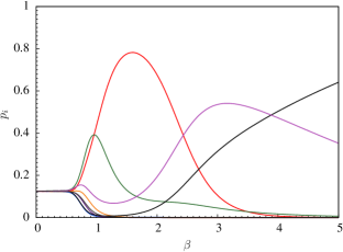
Figure 1: (Color online) A single size $L=10$ sample displaying several boundary-condition crossing. The plot shows the probabilities of the eight boundary conditions $\{p_{i}\}$ as a function of inverse temperature $\beta$.

We carried out simulations of the three-dimensional EA model in TBC using population annealing Monte Carlo Hukushima and Iba (2003); Machta (2010); Machta and Ellis (2011); Wang et al. (2014, 2015). Population annealing is similar to simulated annealing: In both algorithms, the system is cooled from a high temperature to a low temperature following an annealing schedule. However, population annealing involves cooling a population of replicas and includes a resampling of the population as it is cooled. At each temperature step in the annealing schedule, each replica is acted on independently by the Metropolis algorithm. In the resampling step, which occurs before the temperature is changed, replica $i$ is differentially reproduced according to its energy $E_{i}$. The expected number of copies of replica $i$ is $\exp[-(\beta^{\prime}-\beta)E_{i}]/Q(\beta,\beta^{\prime})$ for a temperature step from $\beta$ to $\beta^{\prime}$. The normalization $Q(\beta,\beta^{\prime})$ is chosen such that the expected population size is unchanged by the resampling step, $Q(\beta,\beta^{\prime})=(1/R_{0})\sum_{i}\exp[-(\beta^{\prime}-\beta)E_{i}]$, where $R_{0}$ is the expected population size. The actual number of copies made of replica $i$ is a random integer whose mean is $\exp[-(\beta^{\prime}-\beta)E_{i}]/Q(\beta,\beta^{\prime})$. Note that expected number of copies of each replica is exactly the reweighting factor between Gibbs distributions at $\beta$ and $\beta^{\prime}$. Thus, if the population is representative of the Gibbs distribution at inverse temperature $\beta$ and $R_{0}$ is large, then after resampling, the population is representative the Gibbs distribution at $\beta^{\prime}$. The annealing schedule consists of $N_{T}$ temperature steps equally spaced in $\beta$ with $N_{S}=10$ Metropolis sweeps at each temperature. Thermal boundary conditions are easily simulated in population annealing by initializing the population at $\beta=0$ with $1/8$ of the population in each of the eight BCs Wang et al. (2015). Resampling takes care of making sure that at every temperature, each BC appears with the correct statistical weight. We study $2000$ samples of sizes $L=4$ ($R_{0}=5\,10^{4}$, $N_{T}=101$), $6$ ($R_{0}=2\,10^{5}$, $N_{T}=101$), $8$ ($R_{0}=5\,10^{5}$, $N_{T}=201$), $10$ ($R_{0}=10^{6}$, $N_{T}=301$), and $12$ ($R_{0}=10^{6}$, $N_{T}=301$), down to temperature $T=0.33$. The critical temperature is $T_{c}\approx 0.951$ Katzgraber et al. (2006) so the simulations include temperatures that are deep within the low-temperature phase. For some hard samples Wang et al. (2014) we use larger population sizes. In the case of $L=12$ approximately $300$ samples needed to be run with up to a factor of $10$ larger population sizes.

Using population annealing we carry out a quantitative study of boundary condition crossings. The temperature difference between crossing scales as $L^{-\zeta}$ so that the number of crossing $N_{C}$ in a fixed temperature interval scales as $N_{C}\sim L^{\zeta}$. Also, at crossings, we have that $\Delta F=0$ so that $d_{s}/2$ can be obtained from the scaling of the average of $\Delta E$ at crossings as function of $L$. Finally, in a previous study we measured the stiffness exponent in TBC. We defined the sample stiffness $\lambda$ as $\lambda=\log[f/(1-f)]$ where $f$ is the probability of being in the dominant BC, i.e., $f=\max_{i}[\{p_{i}\}]$. We measured $\theta$ as the scaling of the median of $\lambda$ with system size $L$. Thus, within TBC we can independently measure all three exponents $\theta$, $d_{s}/2$, and $\zeta$ and verify the relation $\zeta=d_{s}/2-\theta$.

Crossings can be divided into two classes: Dominant crossings are those such that the two equal BC probabilities at the crossing are larger than all other BC probabilities. All other crossings are subdominant. For large systems, the BC probability at a subdominant crossing is expected to be typically suppressed by a factor $\exp(L^{-\theta})$ relative to the dominant BC and thus be increasingly difficult to observe in TBC simulations. To avoid finite-size corrections in counting crossings, here we focus on dominant crossings. On the other hand, for measuring $\Delta E=T\Delta S$ ($\Delta S$ the change in entropy) at crossings we do not expect a distinction between dominant and subdominant crossings and, to improve statistics, we use all crossing with $p_{i}>0.05$.

Figure 2 is a log-log plot (base $10$) of $N_{C}$ vs $L$ where $N_{C}$ counts dominant crossing in the range $\beta\in(1.5,3.0)$. A simple power-law fit $N_{C}\sim L^{\zeta}$ yields $\zeta=0.96(5)$. All quoted error bars are one standard deviation statistical errors. To test the effect of temperature on this exponent, we also calculated $\zeta$ from two smaller temperature ranges. For $\beta\in(1.5,2.0)$ we find $\zeta=1.07(8)$, and from $\beta\in(2.0,3.0)$ we find $\zeta=0.85(9)$. For higher temperatures, critical fluctuations may contaminate the measurement of the chaos exponent while for lower temperatures the number of crossings is suppressed by the smallness of the entropy. We note that there is a significant trend to a smaller value of $\zeta$ at lower temperatures. If one assumes that a single exponent holds throughout the low-temperature phase, this trend suggests significant temperature-dependent finite-size corrections. The inset to Fig. 2 shows a histogram of the number of crossings in the range $\beta\in(1.5,3.0)$ with $p_{i}>0.05$ for size $L=12$ as a function of inverse temperature and reveals that the number of crossings decreases with temperature, consistent with the fact that the entropy decreases with temperature so that increasingly large temperature changes are required to change the free-energy difference between BCs. In the large-volume limit, the number of dominant crossings per sample is expected to become infinite but for size $L=12$ temperature chaos events are infrequent but not rare–there are on average $0.86$ crossings with $p_{i}>0.05$ per sample in the range $\beta\in(1.5,3.0)$ and $0.33$ dominant crossings per sample in the same temperature range. An advantage of using boundary condition crossings in TBC is that temperature chaos is not a rare event for accessible system sizes in contrast to overlap correlations in a single boundary condition where chaotic effects are weak in most samples Fernandez et al. (2013).

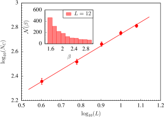
Figure 2: (Color online) Number of dominant crossing in the range $\beta\in(1.5,3.0)$ vs size $L$, for $L=4$, $6$, $8$, $10$, and $12$. The straight line is the best power law fit (see text). The inset is a histogram of the number of all crossings with $p_{i}>0.05$ with respect to $\beta$ for system size $L=12$.

Figure 3 is a log-log plot (base $10$) of the median and mean of the absolute energy difference $|\Delta E|$ vs $L$ at all crossings in the range $\beta\in(1.5,3.0)$ such that $p_{i}>0.05$. A simple power-law fit for the mean yields $|\Delta E|\sim L^{d_{s}/2}$ with $d_{s}/2=1.18(2)$ with the same result for the median. We again test the effect of the temperature range on $d_{s}/2$ by dividing the $\beta$ range into two intervals, $\beta\in(1.5,2.0)$ and $\beta\in(2.0,3.0)$, from which we obtain the the results for the mean $d_{s}/2=1.14(2)$ and $d_{s}/2=1.26(3)$, respectively. There is a significant trend toward larger values at lower temperatures, suggesting temperature-dependent finite-size corrections.

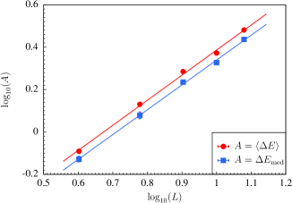
Figure 3: (Color online) Log-log plot of the mean (red circles) and median (blue squares) energy difference between dominant boundary conditions at crossing in the range $\beta\in(1.5,3.0)$ for $L=4$, $6$, $8$, $10$, and $12$. The straight line is the best power law fit (see text). Error bars are smaller than the symbols.

Our results for the three-dimensional EA model, $d_{s}/2=1.17(2)$ and $\zeta=0.96(5)$, are comparable but slightly smaller than previous work: For example, $d_{s}/2=1.29(1)$ was found in Ref. Palassini and Young (2000) based on perturbations of the ground state, and $d_{s}/2=1.31(1)$ was found in Ref. Katzgraber et al. (2001) based on the variance of the link overlap. Recall that our result for $d_{s}/2$ in the lower temperature range is $1.26(3)$, which is within error bars of these zero-temperature results and suggests large temperature-dependent finite-size corrections. Our result, $\zeta=0.96(5)$, is somewhat smaller than $\zeta=1.04$ found in Ref. Katzgraber and Krzakala (2007) from the spin overlap between different temperatures. Combined with our estimate of $\theta=0.27(2)$ Wang et al. (2014) we find that the predicted relation $\zeta=d_{s}/2-\theta$ is reasonably well satisfied by our results.

Temperature chaos partially explains why spin-glass simulations are computationally costly Fernandez et al. (2013). All known efficient algorithms for equilibrating three-dimensional spin glasses rely on coupled simulations at many temperatures. Algorithms in this class include parallel tempering Monte Carlo Hukushima and Nemoto (1996), the Wang-Landau algorithm Wang and Landau (2001), and the algorithm used in this work, population annealing Hukushima and Iba (2003); Machta (2010). In these algorithms, fast mixing at high temperatures provides new configurations to the low-temperature simulations. Temperature chaos decreases the effectiveness of these algorithms because the configurations supplied from higher temperatures are often rather different from the important configurations at lower temperatures. In TBC, temperature chaos means that BCs that are important at high temperature are unimportant at low temperature. This phenomenon is evident in Fig. 1. One might worry that boundary conditions that should be important at low temperature are completely lost at higher temperatures so that the simulations do not reach the correct TBC equilibrium. To verify that this is not the case, we performed an additional check of the equilibration of the TBC ensemble by re-doing several hundred of the hardest $L=12$ samples using an order of magnitude larger population sizes in the simulation and we found no difference in the number of crossings for any sample.

A direct measure of hardness for population annealing for a given sample is the characteristic family size $\rho$. In population annealing, most of the original population is eliminated by successive resampling steps and the final population is descended from a small subset of the initial population. Every member of the final population can be uniquely assigned to a “family” descended from some member of the initial population. Let $n_{i}$ be the fraction of the low-temperature population descended from replica $i$ in the initial population. $\rho$ is then defined as

$$\rho=\lim_{R_{0}\rightarrow\infty}R_{0}\exp\Big{[}\sum_{i}n_{i}\log n_{i}\Big{]},$$ (2)

where $R_{0}$ is the population size in the simulation ($n_{i}=0$ there is no contribution to the sum). In practice, $\rho$ is measured using the large $R_{0}$ of the simulation. Since there may be correlations between members of the same family, the population size $R_{0}$ in the simulation must be much larger than $\rho$ to assure a large number of independent measurements and small statistical errors. Thus samples with the largest $\rho$ require the most computational resources to simulate. We have shown Wang et al. (2014) that $\rho$ is also strongly correlated with the integrated autocorrelation time for parallel tempering Monte Carlo, measured in Ref. Yucesoy et al. (2013) so that the same conclusions are likely to hold for parallel tempering. Figure 4 shows the disorder average of $\log_{10}\rho$ vs $L$ measured at $\beta=3$ for two different classes of disorder samples. The $N_{C}=0$ class has no temperature chaos events (crossings with $p_{i}>0.05$) in the range $\beta\in(1.5,3.0)$ while the $N_{C}>0$ class has one or more temperature chaos events in the same range. The error bars are smaller than the data points and the plots show that $\rho$ scales exponentially in $L$, $\rho\propto\exp(L/\ell)$, for both classes but that the characteristic size scale $\ell=1.27(14)$ is significantly smaller for the chaotic samples than for nonchaotic samples where $\ell=1.62(10)$. It is an interesting question whether temperature chaos slows down all algorithms for spin glasses, not just those that depend on coupling multiple temperatures. Recent studies have shown that Katzgraber et al. (2015); Hen et al. (2015) computationally hard instances for classical algorithms are also computationally hard for quantum annealing machines, like the D-Wave Two quantum annealer. As such, by measuring $\rho$ for a given sample, we have a simple way to uniquely classify the complexity of a given instance. This means that our approach is of great importance in the development of hard problems to discern whether quantum annealing can outperform simulated annealing simulations (see, for example, Refs. Somma et al. (2012); Boixo et al. (2013); Pudenz et al. (2014); Boixo et al. (2014); Rønnow et al. (2014)).

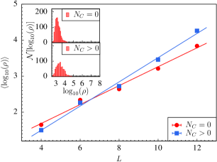
Figure 4: (Color online) The average of the log (base $10$) of the hardness $\rho$, measured at $\beta=3$, vs size $L$ for two classes of samples, those without crossing in the range $\beta\in(1.5,3.0)$, $N_{C}=0$ (red circles) and those with at least one crossing in that range, $N_{C}>0$ (blue squares). Error bars are smaller than the symbols. The insets are histograms of values of $\rho$ for the two classes of samples.

We have seen that thermal boundary conditions allow us to identify temperature chaos with boundary condition crossings and provide a tool for studying chaos quantitatively even for the small sizes accessible to simulations. It would be interesting to apply these ideas to other types of chaos in spin glasses such as bond chaos. We have also established that temperature chaos is a significant determinant of computational hardness for multicanonical algorithms but it remains an open question as to whether temperature chaos is correlated with hardness for all algorithms.