Stability change of a multi-charged vortex due to coupling with quadrupole mode

Abstract

We have studied collective modes of quasi-2D Bose-Einstein condensates with multiply-charged vortices using a variational approach. Two of the four collective modes considered exhibit coupling between the vortex dynamics and the large-scale motion of the cloud. The vortex presence causes a shift in all frequencies of collective modes even for the ones that do not couple dynamically with the vortex-core. The coupling between vortex and large-scale collective excitations can induce the multi-charged vortex to decay into singly-charged vortices with the quadrupole mode being one possible channel for such a decay. Therefore a thorough study was done about the possibility to prevent the vortex decay by applying a Gaussian potential with its width proportional to the vortex-core radius and varying its height. In such way, we created a stability diagram of height versus interaction strength which has stable regions due the static Gaussian potential. Furthermore, by using a sinusoidal time-modulation around the average height of the Gaussian potential, we have obtained a diagram for the parametric resonance which can prevent the vortex decay in regions where static potential can not.

I Introduction

The dynamics of a trapped Bose-Einstein condensate (BEC) containing a vortex line at its center has been the object of our studies. We have studied the effects of a multi-charged vortex in free expansion dynamics. These central vortices contribute with the quantum pressure (kinetic energy) which increases the expansion velocity of the condensate rpteles1 . Consequently, our work culminates in describing the collective excitations of a vortex state as well. Here the vortex-core dynamics couples with the well known collective modes rpteles2 . Furthermore, we shows that it is possible to excite these modes using modulation of the s-wave scattering length. Such a technique has been already applied to excite the lowest-lying quadrupole mode in a lithium experiment cm1 . The motivation for these works is the possibility of experimental realization. Now our focus is in the anisotropic oscillations of the vortex-core. In other words, oscillations that lead the vortex shape from circular to elliptical. Such deformation is a symmetry breaking of vortex state, and can result in changes of dynamical stability.

The presence of vortices in condensates can also shift the frequency of collective excitations. The frequency shift of quadrupole oscillations have been analytically explored for positive scattering lengths by using the sum-role approach smv2 , as well as the effects of lower-dimensional geometry in the frequency splitting of quadrupole oscillations smv3 .

First of all, multi-charged vortices in trapped ultracold Bose gases are thermodynamically unstable, which means that a single $\ell$-charged vortex tends to decay into $\ell$ singly quantized vortices. Thus the configuration of separated singly-charged vortices has lower energy instead a single vortex with the same angular momentum. Although such a state with multiple singly-charged vortices is also thermodynamical unstable when compared with a vortex-free condensate. These multiple vortices spiral outward from the condensate until remain only the ground state.

The vortex dynamic instability has so far been studied in the context of Bogoliubov excitations mcv06 ; mcv07 ; stab03 . Indeed, the vortex state possess certain Bogoliubov eigenmodes which grow exponentially and become unstable against infinitesimal perturbations mcv03 . These vortices present several unstable modes being a quadrupole mode the most unstable. For instance, let us consider the work in Ref.mcv03 . There the authors studied the modes of quadruple-charged vortex. Among of them, only three modes are unstable. These unstable modes have complex eigenfrequencies (CE) and are associated with $l$-fold symmetries. These symmetries are:

• Two-fold symmetry; the quadruply-charged vortex splits into four single vortices arranged in a straight line configuration.

• Three-fold symmetry; the quadruply-charged vortex splits into four single vortices arranged in a triangular configuration, i.e., there are three vortices forming a triangle with each vortex representing a vertex. The fourth one is at center.

• Four-fold symmetry; the quadruply-charged vortex splits into four single vortices arranged in a square configuration with each vortex placed in a vertex.

Our target is to describe them as a result of the coupling between the vortex-core dynamics with the collective modes of the condensate. In order to achieve this goal we have used variational calculations focusing on the description of only one of the unstable mode (specially two-fold symmetry). The variational description becomes very complicated as we increase the number of parameters. Fortunately the most relevant unstable mode is also the easiest one to calculate within the variational approximation.

Furthermore, there are some works which add a static Gaussian potential centered in the core of a vortex with a large circulation which results into a stable configuration for the multi-charged vortex mcv05 ; mcv09 . Based on these works we checked the dynamical stability for a static as well as dynamic potential due to a Gaussian laser beam placed in the vortex-core, when compared with the multiple vortices state.

This paper is organized as follows: In section II, the quasi-2D approach is introduced. We discussed the wave-function used with the variational method in section III and detailed the calculation of the Lagrangian in section IV. Section V contains equations of the motion and their solutions, i.e. the stationary solution, collective modes, and the fully numerical calculation of Gross-Pitaevskii equation (GPE). In section VI, we made a dynamical stability diagram considering a static Gaussian potential while in section VII we made a parametric resonance diagram due to a dynamical Gaussian potential where its height is sinusoidally time dependent.

II Quasi-2d condensate

The presence of a large number of atoms in the ground state allows us to use a classical field description pit-str . Where the non-uniform Bose gas of atomic mass $m$ and s-wave scattering length $a_{s}$. The scattering length is smaller than the average inter-particle distance at absolute zero temperature. Its dynamics is given by the Gross-Pitaevskii equation pethick :

$$i\hbar\frac{\partial\Psi\left(\mathbf{r},t\right)}{\partial t}=\left[-\frac{\hbar^{2}}{2m}\nabla^{2}+V\left(\mathbf{r}\right)+U_{0}\left|\Psi\left(\mathbf{r},t\right)\right|^{2}\right]\Psi\left(\mathbf{r},t\right),$$ (1)

where the interaction strength between two atoms is

$$U_{0}=\frac{4\pi\hbar^{2}a_{s}}{m}.$$ (2)

In order to suppress possible effects due to motions along the axial direction, we consider a highly anisotropic harmonic confinement of the form

$$V\left(\mathbf{r}\right) = V_{\bot}\left(\mathbf{r}_{\bot}\right)+V_{z}\left(z\right)$$ (3)

$$= \frac{1}{2}m\omega_{\rho}^{2}\rho^{2}+\frac{1}{2}m\omega_{z}^{2}z^{2},$$

with $\omega_{z}\gg\omega_{\rho}$. With this condition the condensate wave-function can be separated as a product of radial and axial functions, which are entirely independent. This yields a quasi-2D Bose-Einstein condensate quasi-2D.collisions ; 2Dtempvortex ; smv3 , and leads to

$$\Psi\left(\mathbf{r},t\right)=N\Phi\left(\mathbf{r}_{\bot},t\right)W\left(z,t\right),$$ (4)

where

$$W\left(z,t\right)=\frac{1}{d_{z}\sqrt{\pi}}\exp\left(-\frac{z^{2}}{2d_{z}^{2}}-\frac{i\omega_{z}t}{2}\right).$$ (5)

By replacing (3) and (4) with (5) into the Gross-Pitaevskii equation (1), we obtain

$$i\hbar W\frac{\partial\Phi}{\partial t}+\frac{\hbar\omega_{z}}{2}\Phi W = \left[-\frac{\hbar^{2}}{2m}\nabla_{\bot}^{2}+\frac{\hbar^{2}}{2md_{z}^{2}}-\frac{\hbar^{2}z^{2}}{2md_{z}^{4}}+V\left(\mathbf{r}\right)+NU_{0}\left|\Phi W\right|^{2}\right]\Phi W.$$ (6)

The product $\Phi\left(\mathbf{r}_{\bot},t\right)W\left(z,t\right)$ is normalized to unity, thus the number of atoms appears multiplying the coupling constant $U_{0}$. Now we can multiply Eq. (6) by $W^{*}\left(z,t\right)$ and integrate this equation over the entire z domain. Since $\hbar^{2}/2md_{z}^{2}=\hbar\omega_{z}/2$, and $\hbar^{2}/2md_{z}^{4}=m\omega_{z}^{2}/2$ we obtain the following simplified equation

$$i\hbar\frac{\partial\Phi\left(\mathbf{r}_{\bot},t\right)}{\partial t}=\left[-\frac{\hbar^{2}}{2m}\nabla_{\bot}^{2}+V_{\bot}\left(\mathbf{r}_{\bot}\right)+NU_{2D}\left|\Phi\left(\mathbf{r}_{\bot},t\right)\right|^{2}\right]\Phi\left(\mathbf{r}_{\bot},t\right),$$ (7)

where

$$U_{2D}=\frac{U_{0}}{d_{z}\sqrt{2\pi}}=2\sqrt{2\pi}\frac{\hbar^{2}a_{s}}{md_{z}}.$$ (8)

Let us then write the Lagrangian density which leads to quasi-2D Gross-Pitaevskii equation (7) for a complex field $\Phi\left(\mathbf{r}_{\bot},t\right)$ normalized to unity. So the Lagrangian is given by

$$\mathcal{L}_{2D} = -\frac{i\hbar}{2}\left[\Phi^{*}\left(\mathbf{r}_{\bot},t\right)\frac{\partial\Phi\left(\mathbf{r}_{\bot},t\right)}{\partial t}-\Phi\left(\mathbf{r}_{\bot},t\right)\frac{\partial\Phi^{*}\left(\mathbf{r}_{\bot},t\right)}{\partial t}\right]$$ (9)

$$+\frac{\hbar^{2}}{2m}\left|\nabla_{\bot}^{2}\Phi\left(\mathbf{r}_{\bot},t\right)\right|^{2}+V_{\bot}\left(\mathbf{r}_{\bot}\right)\left|\Phi\left(\mathbf{r}_{\bot},t\right)\right|^{2}+\frac{NU_{2D}}{2}\left|\Phi\left(\mathbf{r}_{\bot},t\right)\right|^{4}.$$

III Breaking wave-function symmetry

In order to examine the coupling between the vortex-core dynamics and the collective modes as well as their stability, we choose the situation where a multi-charged vortex is created at the center of a condensate. Its wave-function can be written in cartesian coordinates as

$$\Phi_{\ell}\left(\mathbf{r}_{\bot},t\right)\propto\left\{1-\frac{1}{\left[x/\xi_{x}\left(t\right)\right]^{2}+2xy/\xi_{xy}\left(t\right)+\left[y/\xi_{y}\left(t\right)\right]^{2}+1}\right\}^{\ell/2}\sqrt{1-\left[\frac{x}{R_{x}\left(t\right)}\right]^{2}-\left[\frac{y}{R_{y}\left(t\right)}\right]^{2}}e^{iS\left(\mathbf{r}_{\bot},t\right)}.$$ (10)

The sizes in each direction are given by $R_{i}\left(t\right)$. They are known as Thomas-Fermi radii, since the wave-function vanishes for $x>R_{x}$ and $y>R_{y}$. The vortex-core sizes are given by $\xi_{i}\left(t\right)$. They are of the order of the healing length for a singly charged vortex. The parameter $\xi_{xy}\left(t\right)$ is responsible for a complete description of the quadrupole symmetries between vortex-core and condensate. The wave-function phase $S\left(\mathbf{r},t\right)$ must be carefully chosen within the context of the variational method. Because the phase must contain the same number of degrees of freedom as the wave-function amplitude. Since we have one pair of variational parameters for each direction in the wave-function amplitude ($\xi_{i}$ and $R_{i}$), we also need a pair of variational parameter in the wave-function phase ($B_{i}$ and $C_{i}$):

$$S\left(\mathbf{r}_{\bot},t\right)=\ell\arctan\left(\frac{y}{x}\right)+B_{x}\left(t\right)\frac{x^{2}}{2}+B_{xy}\left(t\right)xy+B_{y}\left(t\right)\frac{y^{2}}{2}+C_{x}\left(t\right)\frac{x^{4}}{4}+C_{y}\left(t\right)\frac{y^{4}}{4}.$$ (11)

Thus $B_{i}\left(t\right)$ and $C_{i}\left(t\right)$ compose the variations of the condensate velocity field allowing the components $\xi_{i}\left(t\right)$ and $R_{i}\left(t\right)$ to oscillate with opposite directions. While $B_{xy}\left(t\right)$ gives us the contribution of the distortion $\xi_{xy}\left(t\right)$ for velocity field which changes the axis of the quadrupole oscillation. Note that we are not using a parameter which yields a scissor motion to the external components of the condensate, since it has already been shown that such a motion is not coupled with neither breathing nor quadrupole modes scissors1 ; scissor2 .

This choice for our wave-function implies that our vortex-core might have an elliptical shape. It is enough to destabilize a multi-charged vortex and allow it to decay splitting itself into several vortices, each one with unitary charge.

Following the variational method used in Ref. perez1 ; perez2 ; rpteles1 ; rpteles2 , we substituted (10) into (9), and performed the integration over the spacial coordinates, $L_{2D}=\int\mathcal{L}_{2D}d\mathbf{r}_{\bot}$. Although the Lagrangian density (9) cannot be analytically integrated since it does not keep the polar symmetry. One way to proceed is to introduce small fluctuations around the polar-symmetry solutions into the wave-function, and to then to make a Taylor expansion. Thus we can take advantage of the approximate polar symmetry of the vortex-core while the fluctuations act breaking the vortex-core symmetry. These calculations are discussed in detail in the next section.

IV Expanding the Lagrangian around the polar-symmetry solution

Within the Thomas-Fermi approximation the trapping potential shape determines the condensate dimensions. The wavefunction (10) is approximated by an inverted parabola except for the central vortex. So that its integration domain is defined by $1-x^{2}/R_{x}^{2}-y^{2}/R_{y}^{2}\geq 0$. Some care should be taken when calculating the kinetic energy $\left|\nabla_{\bot}\Phi\left(\mathbf{r}_{\bot},t\right)\right|^{2}$ before integrating. The vortex presence inserts an important term in the gradient, while the rest of the gradient is neglected in the Thomas-Fermi approximation. That means that the density varies smoothly along the condensate except in the vortex.

By introducing deviations from the equilibrium position in our parameters

$$\xi_{j}\left(t\right) \approx \xi_{0}+\delta\xi_{j}\left(t\right),$$ (12)

$$R_{j}\left(t\right) \approx R_{0}+\delta R_{j}\left(t\right),$$ (13)

we can expand in Taylor series the deviations of the Lagrangian. In this way we have

$$L=L^{\left(0\right)}+L^{\left(1\right)}+L^{\left(2\right)}+...$$ (14)

The linear approximation is obtained by truncating the series in second order terms, this leads to:

• Terms of zeroth order in $L^{\left(0\right)}$ being responsible for the equilibrium energy per number of atoms.

• Terms of first order $L^{\left(1\right)}$ that vanish due to the stationary solution of Euler-Lagrange equations. The equilibrium configuration has polar symmetry.

• Terms of second order $L^{\left(2\right)}$ carries the collective excitations. Their Euler-Lagrange equations result in a eigensystem whose eigenvectors are composed of deviations ($\delta R_{j}$ and $\delta\xi_{j}$).

Notice that $B_{i}$ and $C_{i}$ from phase (11) also must be considered as first order terms since they lead to deviations in the velocity field. In order to evaluate all the necessary integrals in Eq.(14), it is convenient to use $\xi_{i}\left(t\right)/R_{i}\left(t\right)=\alpha_{i}\left(t\right)$ instead of $\xi_{i}\left(t\right)$. This change is explained due to all these integrals result in functions of $\alpha_{0}=\xi_{0}/R_{0}$. Thus, a we use $\alpha_{i}\left(t\right)\approx\alpha_{0}+\delta\alpha_{i}\left(t\right)$ instead of $\xi_{i}\left(t\right)\approx\xi_{0}+\delta\xi_{i}\left(t\right)$. The same happens for $\alpha_{xy}\left(t\right)=R_{x}\left(t\right)R_{y}\left(t\right)/\xi_{xy}\left(t\right)$ where $\alpha_{xy}\left(t\right)\approx\delta\alpha_{xy}\left(t\right)$. Hereafter we omit the time dependences for simplicity, and we named zeroth order functions as $A_{i}\equiv A_{i}\left(\ell,\alpha_{0}\right)$ as well as the other integrated results as $I_{i}\equiv I_{i}\left(\ell,\alpha_{0}\right)$. Such functions are described in Appendix A.

The proportionality constant in wave-function (10) is found through normalization, being

$$N_{0} = R_{x}^{-1}R_{y}^{-1}\left[A_{0}+I_{1}\left(\delta\alpha_{x}+\delta\alpha_{y}\right)+I_{2}\left(\delta\alpha_{x}^{2}+\delta\alpha_{y}^{2}\right)+I_{3}\delta\alpha_{x}\delta\alpha_{y}+I_{4}\delta\alpha_{xy}^{2}\right]^{-1}$$ (15)

$$\approx R_{x}^{-1}R_{y}^{-1}A_{0}^{-1}\left[1-\frac{I_{1}}{A_{0}}\left(\delta\alpha_{x}+\delta\alpha_{y}\right)+\left(\frac{I_{1}^{2}}{A_{0}^{2}}-\frac{I_{2}}{A_{0}}\right)\left(\delta\alpha_{x}^{2}+\delta\alpha_{y}^{2}\right)\right.$$

$$\left.+\left(\frac{2I_{1}^{2}}{A_{0}^{2}}-\frac{I_{3}}{A_{0}}\right)\delta\alpha_{x}\delta\alpha_{y}-\frac{I_{4}}{A_{0}}\delta\alpha_{xy}^{2}\right].$$

By calculating the Lagrangian integrals we obtain

$$\int\rho^{2}\left|\Phi\right|^{2}d\mathbf{r}_{\bot} = N_{0}R_{x}R_{y}\left\{R_{x}^{2}\left[A_{1}+I_{5}\left(\delta\alpha_{x}+\frac{1}{3}\delta\alpha_{y}\right)+I_{6}\delta\alpha_{x}^{2}+I_{7}\delta\alpha_{y}^{2}+I_{8}\delta\alpha_{x}\delta\alpha_{y}+I_{9}\delta\alpha_{xy}^{2}\right]\right.$$ (16)

$$\left.R_{y}^{2}\left[A_{1}+I_{5}\left(\frac{1}{3}\delta\alpha_{x}+\delta\alpha_{y}\right)+I_{7}\delta\alpha_{x}^{2}+I_{6}\delta\alpha_{y}^{2}+I_{8}\delta\alpha_{x}\delta\alpha_{y}+I_{9}\delta\alpha_{xy}^{2}\right]\right\},$$

$$-i\int\left[\Phi^{*}\frac{\partial\Phi}{\partial t}-\Phi\frac{\partial\Phi^{*}}{\partial t}\right]d\mathbf{r}_{\bot} = N_{0}R_{x}R_{y}\left\{R_{x}^{2}\dot{B_{x}}\left[A_{1}+I_{5}\left(\delta\alpha_{x}+\frac{1}{3}\delta\alpha_{y}\right)\right]\right.$$ (17)

$$+2\dot{B_{xy}}I_{10}\delta\alpha_{xy}+R_{y}^{2}\dot{B_{y}}\left[A_{1}+I_{5}\left(\frac{1}{3}\delta\alpha_{x}+\delta\alpha_{y}\right)\right]$$

$$+\frac{1}{2}R_{x}^{4}\dot{C_{x}}\left[A_{2}+I_{11}\left(\delta\alpha_{x}+\frac{1}{5}\delta\alpha_{y}\right)\right]$$

$$\left.+\frac{1}{2}R_{y}^{4}\dot{C_{y}}\left[A_{2}+I_{11}\left(\frac{1}{5}\delta\alpha_{x}+\delta\alpha_{y}\right)\right]\right\},$$

$$\int\left|\nabla_{\bot}\Phi\right|^{2}d\mathbf{r}_{\bot} = N_{0}R_{x}R_{y}\left\{A_{1}R_{0}^{2}\left(B_{x}^{2}+2B_{xy}^{2}+B_{y}^{2}\right)+2A_{2}R_{0}^{4}\left(B_{x}C_{x}+B_{y}C_{y}\right)+A_{3}R_{0}^{6}\left(C_{x}^{2}+C_{y}^{2}\right)\right.$$ (18)

$$+\frac{\ell^{2}}{R_{x}^{2}}\left[A_{4}+I_{12}\delta\alpha_{x}+I_{13}\delta\alpha_{y}+I_{14}\delta\alpha_{x}^{2}+I_{15}\delta\alpha_{y}^{2}+I_{16}\delta\alpha_{x}\delta\alpha_{y}+I_{17}\delta\alpha_{xy}^{2}\right]$$

$$+\frac{\ell^{2}}{R_{y}^{2}}\left[A_{4}+I_{13}\delta\alpha_{x}+I_{12}\delta\alpha_{y}+I_{15}\delta\alpha_{x}^{2}+I_{14}\delta\alpha_{y}^{2}+I_{16}\delta\alpha_{x}\delta\alpha_{y}+I_{17}\delta\alpha_{xy}^{2}\right]$$

$$+\frac{\ell^{2}}{R_{0}^{2}}\left[A_{5}-\frac{A_{5}}{R_{0}}\left(\delta R_{x}+\delta R_{y}\right)+\frac{A_{5}}{R_{0}^{2}}\left(\delta R_{x}^{2}+\delta R_{y}^{2}+\delta R_{x}\delta R_{y}\right)\right.$$

$$+\frac{I_{18}}{R_{0}}\left(\delta R_{x}\delta\alpha_{x}+\frac{1}{3}\delta R_{x}\delta\alpha_{y}+\frac{1}{3}\delta R_{y}\delta\alpha_{x}+\delta R_{y}\delta\alpha_{y}\right)$$

$$\left.\left.-\frac{2}{3}I_{18}\left(\delta\alpha_{x}+\delta\alpha_{y}\right)+I_{19}\left(\delta\alpha_{x}^{2}+\delta\alpha_{y}^{2}\right)+I_{20}\delta\alpha_{x}\delta\alpha_{y}+I_{21}\delta\alpha_{xy}^{2}\right]\right\},$$

and

$$\int\left|\Phi\right|^{4}d\mathbf{r}_{\bot}=N_{0}^{2}R_{x}R_{y}\left[A_{6}+I_{22}\left(\delta\alpha_{x}+\delta\alpha_{y}\right)+I_{23}\left(\delta\alpha_{x}^{2}+\delta\alpha_{y}^{2}\right)+I_{24}\delta\alpha_{x}\delta\alpha_{y}+I_{25}\delta\alpha_{xy}^{2}\right].$$ (19)

By scaling according to Table 1, each of the three first terms from (14) are given by

$$L^{\left(0\right)}=A_{0}^{-1}\left[A_{1}r_{\rho 0}^{2}+\frac{\ell^{2}}{r_{\rho 0}^{2}}\left(A_{4}+\frac{1}{2}A_{5}\right)\frac{\sqrt{2\pi}\gamma A_{6}}{r_{\rho 0}^{2}A_{0}}\right],$$ (20)

$$L^{\left(1\right)} = \frac{1}{2}A_{0}^{-1}\left[A_{1}r_{\rho 0}^{2}\left(\dot{B_{x}}+\dot{B_{y}}\right)+\frac{1}{2}A_{2}r_{\rho 0}^{4}\left(\dot{C_{x}}+\dot{C_{y}}\right)\right.$$ (21)

$$\left.+S_{\rho}\left(\delta R_{x}+\delta R_{y}\right)+S_{\alpha}\left(\delta\alpha_{x}+\delta\alpha_{y}\right)\right],$$

$$L^{\left(2\right)} = \frac{1}{2}A_{0}^{-1}\left[A_{1}r_{\rho 0}^{2}\dot{\beta}_{x}\left(2\frac{\delta r_{x}}{r_{\rho 0}}+F_{1}\delta\alpha_{x}+F_{2}\delta\alpha_{y}\right)+A_{1}r_{\rho 0}^{2}\dot{\beta}_{y}\left(2\frac{\delta r_{y}}{r_{\rho 0}}+F_{2}\delta\alpha_{x}+F_{1}\delta\alpha_{y}\right)\right.$$ (22)

$$+\frac{1}{2}A_{2}r_{\rho 0}^{4}\dot{\zeta}_{x}\left(4\frac{\delta r_{x}}{r_{\rho 0}}+F_{3}\delta\alpha_{x}+F_{4}\delta\alpha_{y}\right)+\frac{1}{2}A_{2}r_{\rho 0}^{4}\dot{\zeta}_{y}\left(4\frac{\delta r_{y}}{r_{\rho 0}}+F_{4}\delta\alpha_{x}+F_{3}\delta\alpha_{y}\right)$$

$$+A_{1}r_{\rho 0}^{2}\left(\beta_{x}^{2}+\beta_{y}^{2}\right)+2A_{2}r_{\rho 0}^{2}\left(\beta_{x}\zeta_{x}+\beta_{y}\zeta_{y}\right)+A_{3}r_{\rho 0}^{6}\left(\zeta_{x}^{2}+\zeta_{y}^{2}\right)+V_{\rho}\left(\delta r_{x}^{2}+\delta r_{y}^{2}\right)$$

$$+V_{\rho\rho}\delta r_{x}\delta r_{y}+V_{\alpha}\left(\delta\alpha_{x}^{2}+\delta\alpha_{y}^{2}\right)+V_{\alpha\alpha}\delta\alpha_{x}\delta\alpha_{y}+V_{\rho\alpha}\left(\delta r_{x}\delta\alpha_{x}+\delta r_{y}\delta\alpha_{y}\right)$$

$$\left.+V_{\alpha\rho}\left(\delta r_{x}\delta\alpha_{y}+\delta r_{y}\delta\alpha_{x}\right)+2r_{\rho 0}^{2}\left(A_{1}\beta_{xy}^{2}+I_{10}\dot{\beta}_{xy}\delta\alpha_{xy}\right)+V_{xy}\delta\alpha_{xy}^{2}\right],$$

where

$$S_{\rho}=2A_{1}r_{\rho 0}-\frac{\ell^{2}}{r_{\rho 0}^{3}}\left(2A_{4}+A_{5}\right)-\frac{2\sqrt{2\pi}\gamma A_{6}}{r_{\rho 0}^{3}A_{0}},$$ (23)

$$S_{\alpha}=A_{1}r_{\rho 0}^{2}\left(F_{1}+F_{2}\right)+\frac{\ell^{2}}{r_{\rho 0}^{2}}\left[A_{4}\left(F_{5}+F_{6}\right)-A_{5}\left(F_{7}+F_{8}\right)\right]+\frac{2\sqrt{2\pi}\gamma A_{6}}{r_{\rho 0}^{2}A_{0}}F_{9},$$ (24)

$$V_{\rho}=A_{1}+\frac{\ell^{2}}{r_{\rho 0}^{4}}\left(3A_{4}+A_{5}\right)+\frac{2\sqrt{2\pi}\gamma A_{6}}{r_{\rho 0}^{4}A_{0}},$$ (25)

$$V_{\rho\rho}=\frac{\ell^{2}}{r_{\rho 0}^{4}}A_{5}+\frac{2\sqrt{2\pi}\gamma A_{6}}{r_{\rho 0}^{4}A_{0}},$$ (26)

$$V_{\alpha} = A_{1}r_{\rho 0}^{2}\left[\frac{I_{6}+I_{7}}{A_{1}}-2\frac{I_{2}}{A_{0}}-\frac{I_{1}}{A_{0}}\left(F_{1}+F_{2}\right)\right]$$ (27)

$$+\frac{A_{4}\ell}{r_{\rho 0}^{2}}^{2}\left[\frac{I_{14}+I_{15}}{A_{4}}-2\frac{I_{2}}{A_{0}}-\frac{I_{1}}{A_{0}}\left(F_{5}+F_{6}\right)\right]$$

$$+\frac{A_{5}\ell^{2}}{r_{\rho 0}^{2}}\left[\frac{I_{19}}{A_{5}}-\frac{I_{2}}{A_{0}}-\frac{I_{1}}{A_{0}}\left(F_{7}+F_{8}\right)\right]$$

$$+\frac{2\sqrt{2\pi}\gamma A_{6}}{r_{\rho 0}^{2}A_{0}}\left[\frac{I_{23}}{A_{6}}-2\frac{I_{2}}{A_{0}}-\frac{I_{1}}{A_{0}}\left(2F_{9}+\frac{I_{1}}{A_{0}}\right)\right],$$

$$V_{\alpha} = A_{1}r_{\rho 0}^{2}\left[\frac{I_{6}+I_{7}}{A_{1}}-2\frac{I_{2}}{A_{0}}-\frac{I_{1}}{A_{0}}\left(F_{1}+F_{2}\right)\right]$$ (28)

$$+\frac{A_{4}\ell}{r_{\rho 0}^{2}}^{2}\left[\frac{I_{14}+I_{15}}{A_{4}}-2\frac{I_{2}}{A_{0}}-\frac{I_{1}}{A_{0}}\left(F_{5}+F_{6}\right)\right]$$

$$+\frac{A_{5}\ell^{2}}{r_{\rho 0}^{2}}\left[\frac{I_{19}}{A_{5}}-\frac{I_{2}}{A_{0}}-\frac{I_{1}}{A_{0}}\left(F_{7}+F_{8}\right)\right]$$

$$+\frac{2\sqrt{2\pi}\gamma A_{6}}{r_{\rho 0}^{2}A_{0}}\left[\frac{I_{23}}{A_{6}}-2\frac{I_{2}}{A_{0}}-\frac{I_{1}}{A_{0}}\left(2F_{9}+\frac{I_{1}}{A_{0}}\right)\right],$$

$$V_{\alpha\alpha} = 2A_{1}r_{\rho 0}^{2}\left[\frac{I_{8}}{A_{1}}-\frac{I_{3}}{A_{0}}-\frac{I_{1}}{A_{0}}\left(F_{1}+F_{2}\right)\right]$$ (29)

$$+2\frac{A_{4}\ell}{r_{\rho 0}^{2}}^{2}\left[\frac{I_{16}}{A_{4}}-\frac{I_{3}}{A_{0}}-\frac{I_{1}}{A_{0}}\left(F_{5}+F_{6}\right)\right]$$

$$+\frac{A_{5}\ell^{2}}{r_{\rho 0}^{2}}\left[\frac{I_{20}}{A_{5}}-\frac{I_{3}}{A_{0}}+\frac{I_{1}}{A_{0}}\left(F_{7}+F_{8}\right)\right]$$

$$+\frac{2\sqrt{2\pi}\gamma A_{6}}{r_{\rho 0}^{2}A_{0}}\left[\frac{I_{24}}{A_{6}}-2\frac{I_{3}}{A_{0}}-2\frac{I_{1}}{A_{0}}\left(2F_{9}+\frac{I_{1}}{A_{0}}\right)\right],$$

$$V_{\rho\alpha}=2A_{1}r_{\rho 0}F_{1}-\frac{\ell^{2}}{r_{\rho 0}^{3}}\left(2A_{4}F_{5}-A_{5}F_{7}\right)-\frac{2\sqrt{2\pi}\gamma A_{6}}{r_{\rho 0}^{3}A_{0}}F_{9},$$ (30)

$$V_{\alpha\rho}=2A_{1}r_{\rho 0}F_{2}-\frac{\ell^{2}}{r_{\rho 0}^{3}}\left(2A_{4}F_{6}-A_{5}F_{8}\right)-\frac{2\sqrt{2\pi}\gamma A_{6}}{r_{\rho 0}^{3}A_{0}}F_{9},$$ (31)

$$V_{xy} = 2A_{1}r_{\rho 0}^{2}\left(\frac{I_{9}}{A_{1}}-\frac{I_{4}}{A_{0}}\right)+2\frac{A_{4}\ell^{2}}{r_{\rho 0}^{2}}\left(\frac{I_{17}}{A_{4}}-\frac{I_{4}}{A_{0}}\right)$$ (33)

$$+\frac{A_{5}\ell^{2}}{r_{\rho 0}^{2}}\left(\frac{I_{21}}{A_{5}}-\frac{I_{4}}{A_{0}}\right)+\frac{2\sqrt{2\pi}\gamma A_{6}}{r_{\rho 0}^{2}A_{0}}\left(\frac{I_{25}}{A_{6}}-2\frac{I_{4}}{A_{0}}\right),$$

with

$$F_{1} = \frac{I_{5}}{A_{1}}-\frac{I_{1}}{A_{0}},$$ (34)

$$F_{2} = \frac{I_{5}}{3A_{1}}-\frac{I_{1}}{A_{0}},$$ (35)

$$F_{3} = \frac{I_{11}}{A_{2}}-\frac{I_{1}}{A_{0}},$$ (36)

$$F_{4} = \frac{I_{11}}{5A_{2}}-\frac{I_{1}}{A_{0}},$$ (37)

$$F_{5} = \frac{I_{12}}{A_{4}}-\frac{I_{1}}{A_{0}},$$ (38)

$$F_{6} = \frac{I_{13}}{A_{4}}-\frac{I_{1}}{A_{0}},$$ (39)

$$F_{7} = \frac{I_{18}}{A_{5}}-\frac{I_{1}}{A_{0}},$$ (40)

$$F_{8} = \frac{I_{18}}{3A_{5}}-\frac{I_{1}}{A_{0}},$$ (41)

$$F_{9} = \frac{I_{22}}{A_{6}}-2\frac{I_{1}}{A_{0}}.$$ (42)

The terms proportional to $\ell^{2}/r_{\rho 0}^{2}$ and $\ell^{2}/r_{\rho 0}^{3}$ are due to the centrifugal energy added by the multi-charged vortex, and the interaction parameter in dimensionless units is given by $\gamma=Na_{s}/d_{z}$. In the next section, we discuss the Euler-Lagrange equations for the deviations that lead to the four collective modes. Where one of them is dynamically unstable.

	Dimensionless scale
$t$	$\omega_{\rho}^{-1}\tilde{t}$
$\mu$	$\hbar\omega_{\rho}\tilde{\mu}$
$\Omega$	$\omega_{\rho}\tilde{\Omega}$
$R_{0}$	$d_{\rho}r_{\rho 0}$
$\delta R_{j}$	$d_{\rho}\delta r_{j}$
$\xi_{0}$	$d_{\rho}r_{\xi 0}$
$\delta\xi_{j}$	$d_{\rho}\delta r_{\xi j}$
$B_{j}$	$d_{\rho}^{-2}\beta_{j}$
$C_{j}$	$d_{\rho}^{-4}\zeta_{j}$
$\varpi$	$\omega_{\rho}\tilde{\varpi}$

Dimensionless parameters
$\gamma=Na_{s}/d_{z}$
$\alpha=\xi/R$

Table 1: Scale table.

V Energy per atoms, collective modes, and instability of a quadrupole mode

First, in order to calculate both energy per atoms and collective modes, we need to know the equilibrium points $r_{\rho 0}$ and $\alpha_{0}$. They are obtained from Euler-Lagrange equations for $\delta r_{i}$ and $\delta\alpha_{i}$, resulting in

$$S_{\rho}=0,\text{ and }S_{\alpha}=0.$$ (43)

Thus we have different pairs of $r_{\rho 0}$ and $\alpha_{0}$ for each value of $\ell$ and $\gamma$, which are obtained by applying Newton’s method to solve these coupled stationary equations (43). Note that for $\ell=0$ its solution is trivial, given by

$$r_{\rho 0}=2\left(2/\pi\right)^{1/8}\gamma^{1/4}.$$ (44)

These equations (43) do not have physically consistent solutions for low values of $\gamma$ depending on the value of $\ell$, as can be seen in fig.1. We have evaluated the values of the pair $r_{\rho 0}$ and $\alpha_{0}$ for the vortex-states with $\ell=2,4,7$, where the lowest values of interaction are around $\gamma\equiv Na_{s}/d_{z}=29,76,125$, respectively.

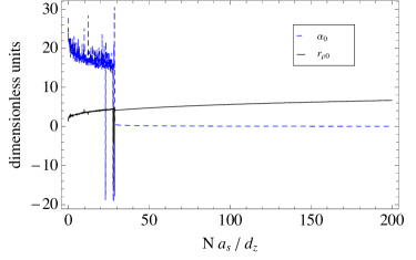
(a) $\ell=2$

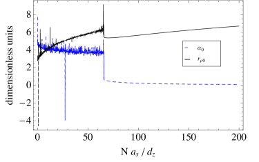
(b) $\ell=4$

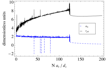
(c) $\ell=7$

Figure 1: (Color online) Equilibrium point of parameters ($r_{\rho 0}$, and $\alpha_{0}$) by atomic interaction. Solid (black) line represents $r_{\rho 0}$, and dashed (blue) line represents $\alpha_{0}$. Both are calculated from (43) where $a_{0}$ must be smaller than $r_{\rho 0}$ and near to zero value. This approach shows itself valid for $Na_{s}/d_{z}>29$ ($Na_{s}/d_{z}>66$, and $Na_{s}/d_{z}>125$) when we have $\ell=2$ ($\ell=4$ and $\ell=7$).

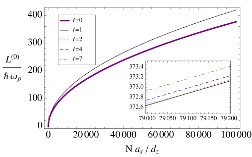
Figure 2: (Color online) Energy per atom as function of interaction parameter.

The energy per atom $L^{\left(0\right)}$ increases proportionally to $\gamma^{1/2}$ being more evident for the vortex-free state ($\ell=0$), where

$$L^{\left(0\right)}=4\left(2/\pi\right)^{1/4}\gamma^{1/2}/3.$$ (45)

We show this behavior for others values of $\ell$ in fig.2. The energy gap between the vortex-free state and the remaining states corresponds to the amount of energy needed to create the $\ell$-charged vortex states. For instance, if a focused laser beam is used to stir a Bose-Einstein condensate in order to nucleate vortices, the stirring frequency must exceeds a critical value vf1, which is defined by difference of energy between the vortex-free state and the singly vortex state.

Calculating the Euler-Lagrange equations from $L^{\left(2\right)}$ we obtain ten coupled equations, being five equations for phase

$$\frac{\dot{\delta r_{x}}}{r_{\rho 0}}+\frac{F_{1}}{2}\dot{\delta\alpha_{x}}+\frac{F_{2}}{2}\dot{\delta\alpha_{y}} = \beta_{x}+\frac{A_{2}}{A_{1}}r_{\rho 0}^{2}\zeta_{x},$$ (46)

$$\frac{\dot{\delta r_{y}}}{r_{\rho 0}}+\frac{F_{2}}{2}\dot{\delta\alpha_{x}}+\frac{F_{1}}{2}\dot{\delta\alpha_{y}} = \beta_{y}+\frac{A_{2}}{A_{1}}r_{\rho 0}^{2}\zeta_{y},$$ (47)

$$\frac{\dot{\delta r_{x}}}{r_{\rho 0}}+\frac{F_{3}}{4}\dot{\delta\alpha_{x}}+\frac{F_{4}}{4}\dot{\delta\alpha_{y}} = \beta_{x}+\frac{A_{3}}{A_{2}}r_{\rho 0}^{2}\zeta_{x},$$ (48)

$$\frac{\dot{\delta r_{y}}}{r_{\rho 0}}+\frac{F_{4}}{4}\dot{\delta\alpha_{x}}+\frac{F_{3}}{4}\dot{\delta\alpha_{y}} = \beta_{y}+\frac{A_{3}}{A_{2}}r_{\rho 0}^{2}\zeta_{y},$$ (49)

$$I_{10}\dot{\delta\alpha_{xy}} = 2A_{1}\beta_{xy},$$ (50)

and other five equations for variational parameter in the amplitude

$$A_{1}r_{\rho 0}\dot{\beta}_{x}+A_{2}r_{\rho 0}^{3}\dot{\zeta}_{x}+2V_{\rho}\delta r_{x}+V_{\rho\rho}\delta r_{y}+V_{\rho\alpha}\delta\alpha_{x}+V_{\alpha\rho}\delta\alpha_{y} \!\!\!\!=\!\!\!\! 0,$$ (51)

$$A_{1}r_{\rho 0}\dot{\beta}_{y}+A_{2}r_{\rho 0}^{3}\dot{\zeta}_{y}+V_{\rho\rho}\delta r_{x}+2V_{\rho}\delta r_{y}+V_{\alpha\rho}\delta\alpha_{x}+V_{\rho\alpha}\delta\alpha_{y} \!\!\!\!=\!\!\!\! 0,$$ (52)

$$A_{1}r_{\rho 0}^{2}\!\left(\!\dot{\beta}_{x}F_{1}\!+\!\dot{\beta}_{y}F_{2}\!\right)\!+\!\frac{1}{2}A_{2}r_{\rho 0}^{4}\!\left(\!\dot{\zeta}_{x}F_{3}\!+\!\dot{\zeta}_{y}F_{4}\!\right)\!+\!V_{\rho\alpha}\delta r_{x}\!+\!V_{\alpha\rho}\delta r_{y}\!+\!2V_{\alpha}\delta\alpha_{x}\!+\!V_{\alpha\alpha}\delta\alpha_{y} \!\!\!\!=\!\!\!\! 0,$$ (53)

$$A_{1}r_{\rho 0}^{2}\!\left(\!\dot{\beta}_{x}F_{2}\!+\!\dot{\beta}_{y}F_{1}\!\right)\!+\!\frac{1}{2}A_{2}r_{\rho 0}^{4}\!\left(\!\dot{\zeta}_{x}F_{4}\!+\!\dot{\zeta}_{y}F_{3}\!\right)\!+\!V_{\alpha\rho}\delta r_{x}\!+\!V_{\rho\alpha}\delta r_{y}\!+\!V_{\alpha\alpha}\delta\alpha_{x}\!+\!2V_{\alpha}\delta\alpha_{y} \!\!\!\!=\!\!\!\! 0,$$ (54)

$$r_{\rho 0}^{2}I_{10}\dot{\beta}_{xy}+V_{xy}\delta\alpha_{xy} \!\!\!\!=\!\!\!\! 0.$$ (55)

We can reduce these ten equations into 4 coupled equations plus one uncoupled equation. The equation for $\delta\alpha_{xy}$ is uncoupled from the others according to

$$\ddot{\delta\alpha_{xy}}+\frac{2A_{1}V_{xy}}{I_{10}^{2}r_{\rho 0}^{2}}\delta\alpha_{xy}=0,$$ (56)

i.e., the motion represented by the deviation $\delta\alpha_{xy}$ is independent of the other collective modes. Those four equations lead to the linearized matrix equation

$$M\ddot{\delta}+V\delta=0,$$

$$\begin{pmatrix}M_{\rho}&0&M_{\rho\alpha}&M_{\alpha\rho}\\ 0&M_{\rho}&M_{\alpha\rho}&M_{\rho\alpha}\\ M_{\rho\alpha}&M_{\alpha\rho}&M_{\alpha}&M_{\alpha\alpha}\\ M_{\alpha\rho}&M_{\rho\alpha}&M_{\alpha\alpha}&M_{\alpha}\end{pmatrix}\begin{pmatrix}\ddot{\delta r_{x}}\\ \ddot{\delta r_{y}}\\ \ddot{\delta\alpha_{x}}\\ \ddot{\delta\alpha_{y}}\end{pmatrix}+\begin{pmatrix}2V_{\rho}&V_{\rho\rho}&V_{\rho\alpha}&V_{\alpha\rho}\\ V_{\rho\rho}&2V_{\rho}&V_{\alpha\rho}&V_{\rho\alpha}\\ V_{\rho\alpha}&V_{\alpha\rho}&2V_{\alpha}&V_{\alpha\alpha}\\ V_{\alpha\rho}&V_{\rho\alpha}&V_{\alpha\alpha}&2V_{\alpha}\end{pmatrix}\begin{pmatrix}\delta r_{x}\\ \delta r_{y}\\ \delta\alpha_{x}\\ \delta\alpha_{y}\end{pmatrix}=0,$$ (57)

where the entries in the matrix $M$ are given by

$$M_{\rho} = 2A_{1},$$ (58)

$$M_{\alpha} = \frac{A_{1}A_{2}^{2}r_{\rho 0}^{2}}{2\left(A_{2}^{2}-A_{1}A_{3}\right)}\left[F_{1}F_{3}+F_{2}F_{4}-\frac{F_{3}^{2}}{4}-\frac{F_{4}^{2}}{4}-\frac{A_{1}A_{3}}{A_{2}^{2}}\left(F_{1}^{2}+F_{2}^{2}\right)\right],$$ (59)

$$M_{\alpha\alpha} = \frac{A_{1}A_{2}^{2}r_{\rho 0}^{2}}{2\left(A_{2}^{2}-A_{1}A_{3}\right)}\left[F_{1}F_{4}+F_{2}F_{3}-\frac{F_{3}F_{4}}{2}-\frac{2A_{1}A_{3}}{A_{2}^{2}}F_{1}F_{2}\right],$$ (60)

$$M_{\rho\alpha} = A_{1}F_{1}r_{\rho 0},$$ (61)

$$M_{\alpha\rho} = A_{1}F_{2}r_{\rho 0}.$$ (62)

Matrix $V$ results from the energy part of the Lagrangian, i.e. from Eqs. (16), (18), and (19). This determinant may be either positive or negative reflecting the system stability. In the other hand, the determinant of $M$ cannot be negative or zero, since it results from our choice for the wave-function phase. The equation (57) seems the Newton’s equation therefore we can say that matrix $M$ has an effect of mass-like, and matrix $V$ works as a potential peristalticmode . Solving the characteristic equation,

$$\det\left(M^{-1}V-\varpi^{2}I\right)=0,$$ (63)

results in the frequencies of the collective modes of oscillation. Eq.(63) is a quartic equation of $\varpi^{2}$. This means that we have four pairs of frequencies $\pm\varpi_{n}^{2}$ being one pair for each oscillatory mode. Among these four modes, two of them have a static vortex representing the collective modes for cloud: they are the breathing mode $B_{c}$, and the quadrupole mode $Q_{c}$. In other words, these modes are similar to collective oscillations of the vortex-free state, where the difference is in a small shift in their frequencies depending on the charge of the vortex, as it is shown in Fig.3. Therefore $B_{c}$ decreases the frequency value while $Q_{c}$ has the opposite effect shifting to higher frequency value. Note that for a vortex-free condensate $\ell=0$, Eq.(63) is a quadratic equation in $\varpi^{2}$. That means the system presents only two modes ($B_{c}$ with $\varpi=2$, and $Q_{c}$ with $\varpi=\sqrt{2}$) in absence of vortex, whose frequencies are constant with respect to the interaction parameter $\gamma$. There are still other two modes which couple vortex dynamics with collective modes. They are another breathing mode $B_{v}$ and another quadrupole mode $Q_{v}$. In this breathing mode $B_{v}$, the vortex-core sizes oscillate out of phase with cloud radii, while $\delta r_{x}$ ($\delta\alpha_{x}$) and $\delta r_{y}$ ($\delta\alpha_{y}$) are in phase. In the quadrupole mode $Q_{v}$, both these sizes $\delta\alpha_{i}$ and $\delta R_{i}$ are oscillating in phase while $\delta r_{x}$ ($\delta\alpha_{x}$) and $\delta r_{y}$ ($\delta\alpha_{y}$) have a $\pi$-phase difference between their oscillations. These modes are sketched in fig.4. The second quadrupole mode $Q_{v}$ has an imaginary frequency (fig.4c), i.e. $Q_{v}$-mode is one possible channel to a multi-charged vortex decay into unitary vortices. Therefore, the multi-charged vortex decay can be explained by the appearance and growth of this unstable quadrupole mode due to quantum or thermal fluctuations. These fluctuations work inducing collective modes, which are coupled to the vortex dynamics through their sound waves.

This model is completely consistent with CE Bogoliubov modes for $\ell=2$, which are composed by only the CE mode associated to two-fold symmetry being our quadrupole mode $Q_{v}$ stab03 . However when $\ell>2$ this calculation is incomplete since we considered only breathing and quadrupole modes. Hence for a complete description it is necessary to add others symmetries for each higher order of $\ell$, which is not a trivial task. Because the Ansatz requires more degrees of freedom, that means we should increase the number of variational parameters.

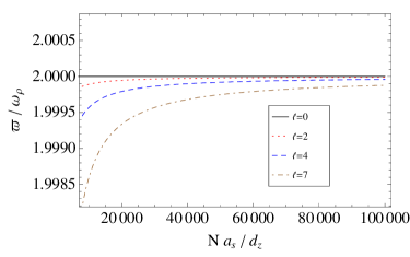
(a) Breathing mode ($B_{c}$)

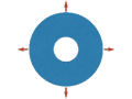
(b) Breathing mode ($B_{c}$)

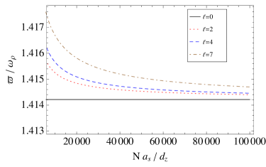
(c) Quadrupole mode ($Q_{c}$)

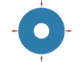
(d) Quadrupole mode ($Q_{c}$)

Figure 3: (Color online) Frequency as functions of interaction parameter with respect to cloud’s collective modes in (a) and (c). These two modes have real frequencies in domain of positive interaction ($Na_{s}/d_{z}>0$). Schematic representation of each collective mode is in (b) and (d).

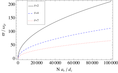
(a) Breathing mode ($B_{v}$)

(b) Breathing mode ($B_{v}$)

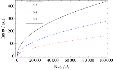
(c) Quadrupole mode ($Q_{v}$)

(d) Quadrupole mode ($Q_{v}$)

Figure 4: (Color online) Frequency as function of interaction parameter for collective modes coupling the dynamics of the vortex-core with the oscillation of atomic cloud radii. Only the quadrupole mode (c) is unstable with imaginary frequency. Schematic representation of collective modes are shown in (b) and (d). $B_{v}$ mode has the vortex core oscillating out of phase with cloud radii. $Q_{v}$ mode is a quadrupole oscillation where vortex core is in phase with cloud radii.

In order to check our results we proceed the full numerical calculation of the Gross-Pitaevskii equation (with the usual phenomenological dissipation $\epsilon$ used since Ref.vortexLatticeFormation ). The reason of this dissipative description is the prevention of non-physical waves created by the grid edge. The initial state is calculated by evolving a trial function in imaginary-time with the parameters given by the equilibrium point from Eq. (43). We introduce the eigenvector from Eq. (57) corresponding to the unstable quadrupole mode ($Q_{v}$). This trial function is given by

$$\Phi_{\ell}\propto\left\{\frac{\left[x/\left(\xi_{0}+\delta\xi_{x}\right)\right]+i\left[y/\left(\xi_{0}+\delta\xi_{y}\right)\right]}{\sqrt{\left[x/\left(\xi_{0}+\delta\xi_{x}\right)\right]^{2}+\left[y/\left(\xi_{0}+\delta\xi_{y}\right)\right]^{2}+1}}\right\}^{\ell}\sqrt{1-\left[\frac{x}{\left(R_{0}+\delta R_{x}\right)}\right]^{2}-\left[\frac{y}{\left(R_{0}+\delta R_{y}\right)}\right]^{2}}.$$ (64)

Furthermore we have done the evolution in real-time where we could check the multi-charged vortex decaying to an initial state containing only the deviations of $Q_{v}$-mode. In figure 5, is shown the evolution of the condensate in real-time for a doubly-charged vortex, such that it starts to split around $\omega_{\rho}t=20.2$. In figure 6, we notice that the life-time of quadruply-charged vortex is around $\omega_{\rho}t=22$. It is necessary to observe that these life-times are different depending on the amplitude of deviations and imaginary-time evolution. It is also possible to induce the decaying by shaping an anisotropic trap, however our semi-analytic approach is valid only for an isotropic trap.

It is interesting to observe the way in which multi-charged vortices decay by $Q_{v}$-mode excitations, which makes the multi-charged vortices split into a straight line of vortices with unitary angular momentum. For instance, we see in figure 6 the quadruply-charged vortex splitting into four vortices and forming a straight line, then evolving based on its interaction with the velocity fields until the final configuration.

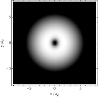
(a) $\omega_{\rho}t=0$

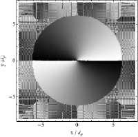
(b) $\omega_{\rho}t=0$

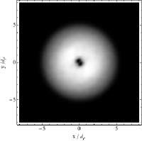
(c) $\omega_{\rho}t=20.2$

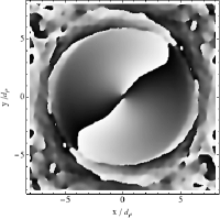
(d) $\omega_{\rho}t=20.2$

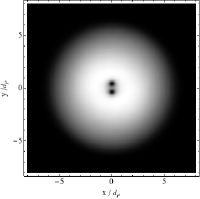
(e) $\omega_{\rho}t=100$

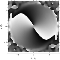
(f) $\omega_{\rho}t=100$

Figure 5: (Color online) Time evolution of the density (a,b,c) and phase (d, e, f) of condensate with a doubly-charged vortex. We have used $\tilde{\mu}=20.198$, $Na_{s}/d_{z}=100$, $\epsilon=0.001$, and a factor of $0.01$ multiplying of the amplitude of deviations.

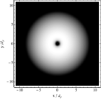
(a) $\omega_{\rho}t=0$

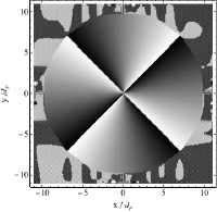
(b) $\omega_{\rho}t=0$

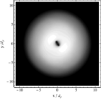
(c) $\omega_{\rho}t=22$

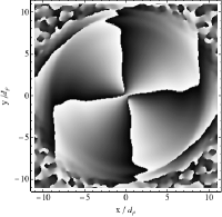
(d) $\omega_{\rho}t=22$

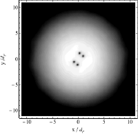
(e) $\omega_{\rho}t=100$

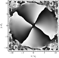
(f) $\omega_{\rho}t=100$

Figure 6: (Color online) Time evolution of the density and phase of condensate with a quadruply-charged vortex. We have used $\tilde{\mu}=45.9552$, $Na_{s}/d_{z}=520$, $\epsilon=0.001$, and a factor of $0.001$ multiplying the amplitude of deviations.

VI Stability diagram due to a static Gaussian potential

Some articles on numerical simulations propose to stabilize an multi-charged vortex by turning on a Gaussian laser beam at the middle of the vortex-core. It means basically that we need to add an external potential with Gaussian shape to the harmonic potential, i.e.

$$V_{\bot}\left(\mathbf{r}_{\bot}\right) = V_{trap}\left(\mathbf{r}_{\bot}\right)+V_{G}\left(\mathbf{r}_{\bot}\right)$$ (65)

$$= \frac{1}{2}m\omega_{\rho}^{2}\rho^{2}+\frac{1}{2}V_{0}e^{-\rho^{2}/\xi_{0}^{2}},$$

where the Gaussian width must be proportional to the vortex-core radius ($w=\sqrt{2}\xi_{0}$). An apparent objection to our approach could lie on the fact that optical resolution limit of a laser beam is around of some microns, while single-charged vortex core is usually smaller than $0.5\text{$\mu$m}$. However, multi-charged vortices may attain much larger sizes depending on its charge, the trap anisotropy, number of atoms, and atomic species. For instance, a quadruply-charged vortex in a ${}^{85}Rb$ condensate ($N=10^{5}$, $a_{s}=100a_{0}$, $\omega_{\rho}=10\text{Hz}$, and $\omega_{z}=100\text{Hz}$) has $5.9\mu m$. By applying a Gaussian beam with $w=10\mu m$ inside of this vortex, its radius grows to $7.1\mu m$. Thus we use this procedure in our semi-analytical method in order to draw a stability diagram, and show that it is enough to stabilize the quadrupole mode $Q_{v}$. So we have to calculate now the Lagrangian part corresponding to the Gaussian potential,

$$L_{G}=\int V_{G}\left(\mathbf{r}_{\bot}\right)\left|\Phi\left(\mathbf{r}_{\bot}\right)\right|^{2}d\mathbf{r}_{\bot}.$$ (66)

By expanding in Taylor series the integral of Gaussian potential $V_{LG}\left(\mathbf{r}_{\bot}\right)$ we have

$$\int e^{-\rho^{2}/\xi_{0}^{2}}\left(\Phi^{*}\Phi\right)d\mathbf{r}_{\bot} = N_{0}R_{x}R_{y}\left[A_{7}+\frac{I_{26}}{R_{0}}\left(\delta R_{x}+\delta R_{y}\right)+\frac{I_{27}}{R_{0}^{2}}\left(\delta R_{x}^{2}+\delta R_{y}^{2}\right)+\frac{I_{28}}{R_{0}^{2}}\delta R_{x}\delta R_{y}\right.$$ (67)

$$+I_{29}\left(\delta\alpha_{x}+\delta\alpha_{y}\right)+I_{30}\left(\delta\alpha_{x}^{2}+\delta\alpha_{y}^{2}\right)+I_{31}\delta\alpha_{x}\delta\alpha_{y}$$

$$\left.\!\!\!\!\!\!+\frac{I_{32}}{R_{0}}\left(\delta R_{x}\delta\alpha_{x}+\delta R_{y}\delta\alpha_{y}\right)+\frac{I_{33}}{R_{0}}\left(\delta R_{x}\delta\alpha_{y}+\delta R_{y}\delta\alpha_{x}\right)+I_{34}\delta\alpha_{xy}^{2}\right],$$

where Lagrangian part becomes

$$L_{G} = -\frac{\tilde{V}_{0}A_{7}}{2A_{0}}\left\{1+\frac{I_{26}}{A_{7}R_{0}}\left(\delta R_{x}+\delta R_{y}\right)+\frac{I_{27}}{A_{7}R_{0}^{2}}\left(\delta R_{x}^{2}+\delta R_{y}^{2}\right)\right.$$ (68)

$$+\frac{I_{28}}{A_{7}R_{0}^{2}}\delta R_{x}\delta R_{y}+\left(\frac{I_{29}}{A_{7}}-\frac{I_{1}}{A_{0}}\right)\left(\delta\alpha_{x}+\delta\alpha_{y}\right)$$

$$+\left[\frac{I_{30}}{A_{7}}-\frac{I_{2}}{A_{0}}-\frac{I_{1}}{A_{0}}\left(\frac{I_{29}}{A_{7}}-\frac{I_{1}}{A_{0}}\right)\right]\left(\delta\alpha_{x}^{2}+\delta\alpha_{y}^{2}\right)$$

$$+\left[\frac{I_{31}}{A_{7}}-\frac{I_{3}}{A_{0}}-2\frac{I_{1}}{A_{0}}\left(\frac{I_{29}}{A_{7}}-\frac{I_{1}}{A_{0}}\right)\right]\delta\alpha_{x}\delta\alpha_{y}$$

$$+\frac{1}{R_{0}}\left(\frac{I_{32}}{A_{7}}-\frac{I_{26}I_{1}}{A_{7}A_{0}}\right)\left(\delta R_{x}\delta\alpha_{x}+\delta R_{y}\delta\alpha_{y}\right)$$

$$\left.+\frac{1}{R_{0}}\left(\frac{I_{33}}{A_{7}}-\frac{I_{26}I_{1}}{A_{7}A_{0}}\right)\left(\delta R_{x}\delta\alpha_{y}+\delta R_{y}\delta\alpha_{x}\right)+\left(\frac{I_{34}}{A_{7}}-\frac{I_{4}}{A_{0}}\right)\delta\alpha_{xy}^{2}\right\}.$$

Notice that we have terms of first order in deviations in Eq. (68), it means that the stationary solution is modified when the condensate is under the influence of a Gaussian potential. The first-order contribution in (68) becomes

$$L_{G}^{\left(1\right)}=-\frac{\tilde{V}_{0}A_{7}}{2A_{0}}\left\{\overset{s_{\rho}}{\overbrace{\frac{I_{26}}{A_{7}R_{0}}}}\left(\delta R_{x}+\delta R_{y}\right)+\overset{s_{\alpha}}{\overbrace{\left(\frac{I_{29}}{A_{7}}-\frac{I_{1}}{A_{0}}\right)}}\left(\delta\alpha_{x}+\delta\alpha_{y}\right)\right\},$$ (69)

while the second-order terms are

$$L_{G}^{\left(2\right)} = -\frac{\tilde{V}_{0}A_{7}}{2A_{0}}\left\{\stackrel{{\scriptstyle p_{\rho}}}{{\overbrace{\frac{I_{27}}{A_{7}R_{0}^{2}}}}}\left(\delta R_{x}^{2}+\delta R_{y}^{2}\right)+\stackrel{{\scriptstyle p_{\rho\rho}}}{{\overbrace{\frac{I_{28}}{A_{7}R_{0}^{2}}}}}\delta R_{x}\delta R_{y}\right.$$ (70)

$$+\stackrel{{\scriptstyle p_{\alpha}}}{{\overbrace{\left[\frac{I_{30}}{A_{7}}-\frac{I_{2}}{A_{0}}-\frac{I_{1}}{A_{0}}\left(\frac{I_{29}}{A_{7}}-\frac{I_{1}}{A_{0}}\right)\right]}}}\left(\delta\alpha_{x}^{2}+\delta\alpha_{y}^{2}\right)$$

$$+\stackrel{{\scriptstyle p_{\alpha\alpha}}}{{\overbrace{\left[\frac{I_{31}}{A_{7}}-\frac{I_{3}}{A_{0}}-2\frac{I_{1}}{A_{0}}\left(\frac{I_{29}}{A_{7}}-\frac{I_{1}}{A_{0}}\right)\right]}}}\delta\alpha_{x}\delta\alpha_{y}$$

$$+\stackrel{{\scriptstyle p_{\rho\alpha}}}{{\overbrace{\frac{1}{R_{0}}\left(\frac{I_{32}}{A_{7}}-\frac{I_{26}I_{1}}{A_{7}A_{0}}\right)}}}\left(\delta R_{x}\delta\alpha_{x}+\delta R_{y}\delta\alpha_{y}\right)$$

$$\left.+\stackrel{{\scriptstyle p_{\alpha\rho}}}{{\overbrace{\frac{1}{R_{0}}\left(\frac{I_{33}}{A_{7}}-\frac{I_{26}I_{1}}{A_{7}A_{0}}\right)}}}\left(\delta R_{x}\delta\alpha_{y}+\delta R_{y}\delta\alpha_{x}\right)\right\}.$$

The equilibrium points are changed to

$$S_{\rho}+s_{\rho}=0,\text{ and }S_{\alpha}+s_{\alpha}=0.$$ (71)

Each terms in (70) adds a contribution to a different element in the matrix $V$ of the linearized Euler-Lagrange equation (57) which then becomes

$$M\ddot{\delta}+\left(V+V_{G}\right)\delta=0,$$ (72)

where

$$V_{G}=\frac{\tilde{V}_{0}A_{7}}{2A_{0}}\begin{pmatrix}2p_{\rho}&p_{\rho\rho}&p_{\rho\alpha}&p_{\alpha\rho}\\ p_{\rho\rho}&2p_{\rho}&p_{\alpha\rho}&p_{\rho\alpha}\\ p_{\rho\alpha}&p_{\alpha\rho}&2p_{\alpha}&p_{\alpha\alpha}\\ p_{\alpha\rho}&p_{\rho\alpha}&p_{\alpha\alpha}&2p_{\alpha}\end{pmatrix}.$$ (73)

Since the stability of the eigensystem depends only on the $Q_{v}$-frequency, we can build a stability diagram of $V_{0}/\hbar\omega_{\rho}$ versus $Na_{s}/d_{z}$. In fig.7, this diagram is shown considering two cases, $\ell=2$ and $\ell=4$. As the angular momentum $\ell$ gets larger the stable region decreases. Hence the pinning potential can prevent the vortices from splitting for some values of $V_{0}/\hbar\omega_{\rho}$ depending on $Na_{s}/d_{\rho}$.

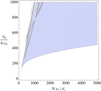
(a) $\ell=2$

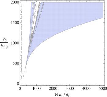
(b) $\ell=4$

Figure 7: (Color online) Diagram of magnitude of pinning potential by atomic interaction for vortex with $\ell=2$ and $\ell=4$. Hatched region represents stable eigensystem meaning the vortex-core become stable.

In order to validate these stability diagrams, we make a numerical simulation of the Gross-Pitaevskii equation. When the Gaussian potential is turned on, we have seen that it provokes some phonon-waves on the condensate surface and increases a little the vortex-core size besides preventing the vortex decay. Figure 8 shows phonon-waves rising and vanishing due to dissipation. The same phenomena may be seen in figure 9.

The vortex decay happens when the sound waves couple the quadrupole mode from the edge of the condensate with the vortex-core, which breaks the polar symmetry of vortex. Therefore, the pinning potential acts as a wall reflecting these sound waves, and preventing the vortex symmetry break.

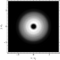
(a) $\omega_{\rho}t=1$

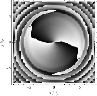
(b) $\omega_{\rho}t=1$

(c) $\omega_{\rho}t=21$

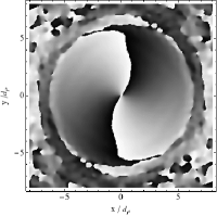
(d) $\omega_{\rho}t=21$

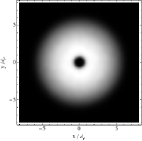
(e) $\omega_{\rho}t=100$

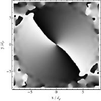
(f) $\omega_{\rho}t=100$

Figure 8: (Color online) Time evolution of the density (a, c, e) and phase (b, d, f) of condensate with a doubly-charged vortex. We used $\mu/\hbar\omega_{\rho}=20.198$, $Na_{s}/d_{z}=100$, $V_{0}/\hbar\omega_{\rho}=150$, $\epsilon=0.001$, and a factor of $0.01$ multiplying the amplitude of deviations.

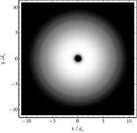
(a) $\omega_{\rho}t=1$

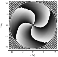
(b) $\omega_{\rho}t=1$

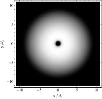
(c) $\omega_{\rho}t=22$

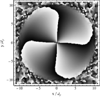
(d) $\omega_{\rho}t=22$

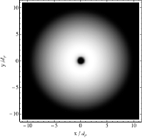
(e) $\omega_{\rho}t=100$

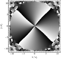
(f) $\omega_{\rho}t=100$

Figure 9: (Color online) Time evolution of the density (a, c, e) and phase (b, d, f) of condensate with a quadruply-charged vortex. We used $\mu/\hbar\omega_{\rho}=45.9552$, $Na_{s}/d_{z}=520$, $V_{0}/\hbar\omega_{\rho}=500$, $\epsilon=0.001$, and a factor of $0.001$ multiplying the amplitude of deviations.

VII Diagram of stability due to a dynamic Gaussian potential

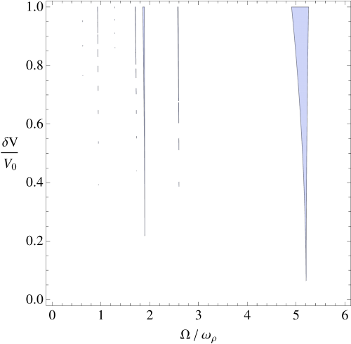
Figure 10: (Color online) Diagram of amplitude versus frequency where hatched stable regions are found for a condensate containing a triply-charged vortex subjected to height modulation. We used $Na_{s}/d_{z}=125$. Convergence is obtained already with two iterations.

In section VI, we have seen that it is possible to make a multi-charged vortex stable using a static Gaussian potential. In addition, we calculated a diagram of height versus interaction strength which shows the stable region. Here we propose to stabilize a multi-charged vortex with a sinusoidal modulation of height of the Gaussian potential with an amplitude given by $\delta V$,

$$V_{0}\left(t\right)=V_{0}-\delta V\cos\left(\Omega t\right),$$ (74)

at the specific region of interaction strength where the static potential is not capable of stabilizing the vortex, i.e. $0<Na_{s}/d_{\rho}\leq 160$. The equation for this case is given by

$$M\ddot{\delta}+\left\{V+V_{G}\left[1-\frac{\delta V}{V_{0}}\cos\left(\tilde{\Omega}\tilde{t}\right)\right]\right\}\delta=0,$$ (75)

where matrices $M$ and $V$ can be found at Eq.(57), and $V_{LG}$ is given by Eq.(73). By scaling the time as follows

$$\frac{\Omega}{\omega_{\rho}}\tilde{t}\rightarrow 2\tau,$$ (76)

we obtain the Mathieu equation

$$\frac{\tilde{\Omega}^{2}}{4}\ddot{\delta}+\left\{A-2\frac{\delta V}{V_{0}}Q\cos\left(2\tau\right)\right\}\delta=0,$$ (77)

where $A=M^{-1}\left(V+V_{LG}\right)$ and $Q=\left(1/2\right)M^{-1}V_{LG}$ are constants depending on the initial conditions. This equation becomes solvable by using Floquet theory mathieu1 ; mathieu2 ; floquet ; Floquet1 ; Floquet2 . The basic idea of this theory is that if a linear differential equation has periodic coefficients, the solutions will be a linear periodic combination of functions times exponentially increasing (or decreasing) functions. Thus linear independent solutions of the Mathieu equation for any pair of $A$ and $B$ can be expressed as

$$\delta\left(\tau\right)=e^{\pm\eta\tau}P\left(\pm\tau\right),$$ (78)

where $\eta$ is called the characteristic exponent which is a constant depending on both $A$ and $Q$, and $P\left(\tau\right)$ is $\pi$-periodic in $\tau$ that which can be written as an infinity series

$$\delta\left(\tau\right)=e^{\eta\tau}\sum_{n=-\infty}^{\infty}b_{2n}e^{2ni\tau},$$ (79)

with $b_{2n}$ being a Fourier component. Doing the substitution of (79) into (77), we have

$$\left[A+\frac{\tilde{\Omega}^{2}}{4}\left(\eta+2ni\right)^{2}I\right]b_{2n}-Q\left(b_{2n+2}+b_{2n-2}\right)=0.$$ (80)

At this point it is wise to define ladder operators $L_{2n}^{\pm}b_{2n}=b_{2n\pm 2}$ which yields

$$L_{2n}^{\pm}=\left\{A+\frac{\tilde{\Omega}^{2}}{4}\left[\eta+2i\left(n\pm 1\right)\right]^{2}I-QL_{2n\pm 2}^{\pm}\right\}^{-1}Q.$$ (81)

By using (81) to write (80) in terms of $b_{0}$ only, we obtain an iteration algorithm wherein we replace the ladder operator over and over inside itself which then becomes

$$\left(A+\frac{\tilde{\Omega}^{2}}{4}\eta^{2}I-Q\left\{\left[A+\frac{\tilde{\Omega}^{2}}{4}\left(\eta+2i\right)^{2}I-\cdots\right]^{-1}\right.\right.$$

$$\left.\left.+\left[A+\frac{\tilde{\Omega}^{2}}{4}\left(\eta-2i\right)^{2}I-\cdots\right]^{-1}\right\}Q\right)b_{0} = 0.$$ (82)

Since we are not interested in trivial solutions for $b_{0}$, the determinant of (82) must vanish. Thus the stability diagram for a modulation of the Gaussian potential with frequency $\Omega$ and amplitude $V_{0}$ is presented in fig. 10, where its resonant behavior does not depend on the initial conditions PR1 .

The edges between stable and unstable domains (also called as Floquet fringes) were calculated by making $\eta=0$. Since the equilibrium configuration rarely has solution for $V_{0}/\hbar\omega_{\rho}\geq Na_{s}/d_{z}$, we only build the stability diagram for $V_{0}/\hbar\omega_{\rho}<Na_{s}/d_{z}$. The iterative algorithm converges very fast, and does not require more than two iterations.

The stable regions, also called resonance region, can lead the system to lose coherence if the excitation time is long enough (hundreds of milliseconds according to number of atoms) which leads to destruction of the condensate state.

The dynamical mechanism works exciting the resonant mode by the oscillatory potential placed at the center of the condensate that suppresses completely the $Q_{v}$-mode, when the correct frequency and amplitude are considered. Since this mode no longer exists, the vortex becomes stable (Fig.11). It is what happens for the case where the static potential cannot stabilize the vortex by itself. On the other hand, in the case of static potential is enough to prevent the vortex decay, the modulation of the height plays an opposite role inducing the vortex decay in resonance regions.

(a) $\omega_{\rho}t=14$

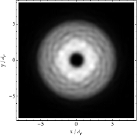
(b) $\omega_{\rho}t=14$

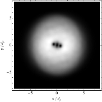
(c) $\omega_{\rho}t=19$

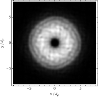
(d) $\omega_{\rho}t=19$

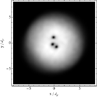
(e) $\omega_{\rho}t=100$

(f) $\omega_{\rho}t=100$

Figure 11: (Color online) Time evolution of condensate density with a triply-charged vortex for both free Gaussian potential (a, c, e) and dynamical potential (b, d, f). We used $\mu/\hbar\omega_{\rho}=20$, $Na_{s}/d_{z}=125$, $V_{0}/\hbar\omega_{\rho}=50$, $\delta V/V_{0}=0.5$, $\Omega/\omega_{\rho}=5.2$, $\epsilon=0.001$, and a factor of 0.01 multiplying the amplitude of deviations.

VIII Conclusions

In this paper we have studied the stability of collective modes as well as its dynamical stability for a quasi-2D Bose-Einstein condensate with a multi-charged vortex. The presence of a $\ell$-charged vortex causes a shift in the frequencies of the cloud collective modes, however such changes are not substantial. The vortex rotational mode is an independent degree of freedom and does not affect vortex stability. The vortex dynamics couples with collective excitations, and it can be the cause for the $\ell$-charged vortex decay. Its decay has as responsible the quadrupole oscillation $Q_{v}$, which is one channel that leads the $\ell$-charged vortex to decay into $\ell$ singly vortices. This quadrupole is the main channel to doubly-charged vortex decay into two singly vortices. By applying a static Gaussian potential we can prevent the decay of a vortex for specific potential amplitudes, whereas for some regions in the parameter space can be stabilized by a time periodic modulation of the laser potential.

Appendix A Functions $A_{i}\left(\ell,\alpha_{0}\right)$ and $I_{i}\left(\ell,\alpha_{0}\right)$

Similar functions to $A_{i}\left(\ell,\alpha_{0}\right)$ for a 3D case have been calculated in Ref.rpteles2 . Since it is a Thomas-Fermi wave-function the procedure to evaluate each integral is the same, where we start changing the scale of both $x$ and $y$ coordinates according to $x\rightarrow R_{x}x$ and $y\rightarrow R_{y}y$. By doing this $\xi_{i}$ becomes $\alpha_{i}=\xi_{i}/R_{i}$, i.e. the integral becomes dimensionless. Now it is convenient to change the coordinates from cartesians to polar ($x=\rho\cos\phi$ and $y=\rho\sin\phi$) where the integration domains are $0\leq\rho\leq 1$ and $0\leq\phi\leq 2\pi$, in this way we have

$$A_{0}\left(\ell,\alpha_{0}\right)=\frac{\pi}{\alpha_{0}^{2\ell}}\left[\frac{{}_{2}F_{1}\left(\ell,\ell+1;\ell+2;-\alpha_{0}^{-2}\right)}{\ell+1}-\frac{{}_{2}F_{1}\left(\ell,\ell+2;\ell+3;-\alpha_{0}^{-2}\right)}{\ell+2}\right],$$ (83)

$$A_{1}\left(\ell,\alpha_{0}\right)=\frac{1}{2}\left(-1\right)^{\ell}\pi\alpha_{0}^{4}\left[B\left(-\alpha_{0}^{-2};\ell+2,\ell-1\right)+\alpha_{0}^{2}B\left(-\alpha_{0}^{-2};\ell+3,\ell-1\right)\right],$$ (84)

$$A_{2}\left(\ell,\alpha_{0}\right)=\frac{3}{8}\pi\alpha_{0}^{-2\ell}\left[\frac{{}_{2}F_{1}\left(\ell,\ell+3;\ell+4;-\alpha_{0}^{-2}\right)}{\ell+3}-\frac{{}_{2}F_{1}\left(\ell,\ell+4;\ell+5;-\alpha_{0}^{-2}\right)}{\ell+4}\right],$$ (85)

$$A_{3}\left(\ell,\alpha_{0}\right)=\frac{5}{16}\left(-1\right)^{\ell}\pi\alpha_{0}^{8}\left[B\left(-\alpha_{0}^{-2};\ell+4,\ell-1\right)+\alpha_{0}^{2}B\left(-\alpha_{0}^{-2};\ell+5,\ell-1\right)\right],$$ (86)

$$A_{4}\left(\ell,\alpha_{0}\right)=\frac{\pi\left(1+\alpha_{0}^{2}\right)^{-\ell}}{2\ell\left(1+\ell\right)},$$ (87)

$$A_{5}\left(\ell,\alpha_{0}\right)=\frac{\pi}{\alpha_{0}^{2\ell}}\left[\frac{{}_{2}F_{1}\left(\ell,\ell;\ell+1;-\alpha_{0}^{-2}\right)}{\ell}-\frac{{}_{2}F_{1}\left(\ell,\ell+1;\ell+2;-\alpha_{0}^{-2}\right)}{\ell+1}\right],$$ (88)

$$A_{6}\left(\ell,\alpha_{0}\right)=\frac{\pi}{\alpha_{0}^{4\ell}}\left[\frac{{}_{2}F_{1}\left(2\ell,2\ell+1;2\ell+2;-\alpha_{0}^{-2}\right)}{2\ell+1}-\frac{{}_{2}F_{1}\left(2\ell,2\ell+2;2\ell+3;-\alpha_{0}^{-2}\right)}{2\ell+2}\right],$$ (89)

$$I_{1}\left(\ell,\alpha_{0}\right)=\pi\ell\alpha_{0}\left\{\left(1+\alpha_{0}^{2}\right)^{-\ell}+\left(-1\right)^{\ell}\left[1+\left(1+\ell\right)\alpha_{0}^{2}\right]B\left(-\alpha_{0}^{-2};\ell+1,-\ell\right)\right\},$$ (90)

$$I_{2}\left(\ell,\alpha_{0}\right)=\frac{3}{4}\pi\ell\left[\left(1+\alpha_{0}^{2}\right)^{-\ell-1}-\left(\frac{\ell+1}{\alpha_{0}^{2\ell+2}}\right)\frac{{}_{2}F_{1}\left(\ell+2,\ell+2;\ell+3;-\alpha_{0}^{-2}\right)}{\ell+2}\right],$$ (91)

$$I_{3}\left(\ell,\alpha_{0}\right) = \frac{\pi\ell}{2\alpha_{0}^{2\ell+2}}\left[\left(\frac{1+3\ell}{\ell+1}\right)\left(1+\alpha_{0}^{-2}\right)^{-\ell-1}\right.$$ (92)

$$\left.-\left(\frac{2}{\alpha_{0}^{2}}+3\ell+3\right)\frac{{}_{2}F_{1}\left(\ell+2,\ell+2;\ell+3;-\alpha_{0}^{-2}\right)}{\ell+2}\right],$$

$$I_{4}\left(\ell,\alpha_{0}\right) = \frac{\pi\ell}{4\alpha_{0}^{2\ell-4}}\left[\left(\frac{3\ell+1}{\ell+1}\right)\left(1+\alpha_{0}^{-2}\right)^{-\ell-1}\right.$$ (93)

$$\left.-\left(\frac{2}{\alpha_{0}^{2}}+3\ell+3\right)\frac{{}_{2}F_{1}\left(\ell+2,\ell+2;\ell+3;-\alpha_{0}^{-2}\right)}{\ell+2}\right],$$

$$I_{5}\left(\ell,\alpha_{0}\right)=-\frac{3}{4}\left(-1\right)^{\ell}\pi\alpha_{0}^{3}\left[B\left(-\alpha_{0}^{-2};\ell+2,-\ell\right)+\alpha_{0}^{2}B\left(-\alpha_{0}^{-2};\ell+3,-\ell\right)\right]$$ (94)

$$I_{6}\left(\ell,\alpha_{0}\right) = \frac{\pi\ell}{16\alpha_{0}^{2\ell}}\left\{\left[\frac{11\left(2\ell+1\right)+12\alpha_{0}^{-2}}{\left(\ell+1\right)^{-1}}\right]\frac{{}_{2}F_{1}\left(\ell+2,\ell+2;\ell+3;-\alpha_{0}^{-2}\right)}{\ell+2}\right.$$ (95)

$$\left.-\frac{\alpha_{0}^{-2}+11\left(\ell+1\right)}{\left(1+\alpha_{0}^{-2}\right)^{\ell+1}}\right\},$$

$$I_{7}\left(\ell,\alpha_{0}\right)=\frac{\pi\ell}{16\alpha_{0}^{2\ell}}\left[\frac{{}_{2}F_{1}\left(\ell+2,\ell+2;\ell+3;-\alpha_{0}^{-2}\right)}{\left(\ell+1\right)^{-1}}-\frac{\ell+1-\alpha_{0}^{-2}}{\left(1+\alpha_{0}^{-2}\right)^{\ell+1}}\right],$$ (96)

$$I_{8}\left(\ell,\alpha_{0}\right) = \frac{\pi\ell}{4\alpha_{0}^{2\ell}}\left\{\left[\frac{2\ell+4+3\alpha_{0}^{-2}}{\left(\ell+1\right)^{-1}}\right]\frac{{}_{2}F_{1}\left(\ell+2,\ell+2;\ell+3;-\alpha_{0}^{-2}\right)}{\ell+2}\right.$$ (97)

$$\left.-\frac{\alpha_{0}^{-2}+2\ell+2}{\left(1+\alpha_{0}^{-2}\right)^{\ell+1}}\right\},$$

$$I_{9}\left(\ell,\alpha_{0}\right) = \frac{\pi\ell}{8\alpha_{0}^{2\ell-6}}\left[\left(\ell+1\right)\left(\frac{3}{\alpha_{0}^{2}}+4+2\ell\right)\frac{{}_{2}F_{1}\left(\ell+2,\ell+2;\ell+3;-\alpha_{0}^{-2}\right)}{\ell+2}\right.$$ (98)

$$\left.-\frac{\alpha_{0}^{-2}+2\ell+2}{\left(1+\alpha_{0}^{-2}\right)^{\ell+1}}\right],$$

$$I_{10}\left(\ell,\alpha_{0}\right)=\!\frac{\pi\ell}{4\alpha_{0}^{2\ell-2}}\!\!\left[\!\frac{{}_{2}F_{1}\left(\ell+1,\ell+2;\ell+3;-\alpha_{0}^{-2}\right)}{\ell+2}\!-\!\frac{{}_{2}F_{1}\left(\ell+1,\ell+3;\ell+4;-\alpha_{0}^{-2}\right)}{\ell+3}\!\right]\!\!,$$ (99)

$$I_{11}\left(\ell,\alpha_{0}\right)=\frac{5}{8}\left(-1\right)^{\ell}\pi\ell\alpha_{0}^{5}\left[B\left(-\alpha_{0}^{-2};\ell+3,-\ell\right)+\alpha_{0}^{2}B\left(-\alpha_{0}^{-2};\ell+4,-\ell\right)\right],$$ (100)

$$I_{12}\left(\ell,\alpha_{0}\right)=\frac{\pi}{4}\frac{2\alpha_{0}^{-1}+\left(3\ell+2\right)\alpha_{0}}{\ell\left(\ell+1\right)\left(1+\alpha_{0}^{2}\right)^{\ell+1}},$$ (101)

$$I_{13}\left(\ell,\alpha_{0}\right)=\frac{\pi}{4}\frac{2\alpha_{0}^{-1}-\left(\ell-2\right)\alpha_{0}}{\ell\left(\ell+1\right)\left(1+\alpha_{0}^{2}\right)^{\ell+1}},$$ (102)

$$I_{14}\left(\ell,\alpha_{0}\right)=\frac{\pi}{8}\frac{3\ell+8+4\alpha_{0}^{-2}+\left[4+\ell\left(5\ell+8\right)\right]\alpha_{0}^{2}}{\ell\left(\ell+1\right)\left(1+\alpha_{0}^{2}\right)^{\ell+2}},$$ (103)

$$I_{15}\left(\ell,\alpha_{0}\right)=\frac{\pi}{8}\frac{\left(\ell-2\right)\alpha_{0}^{2}-3}{\left(\ell+1\right)\left(1+\alpha_{0}^{2}\right)^{\ell+2}},$$ (104)

$$I_{16}\left(\ell,\alpha_{0}\right)=\frac{\pi}{4}\frac{\left(\ell^{2}-\ell+2\right)\alpha_{0}^{2}-2\alpha_{0}^{-2}-2\ell-4}{\ell\left(\ell+1\right)\left(1+\alpha_{0}^{2}\right)^{\ell+2}},$$ (105)

$$I_{17}\left(\ell,\alpha_{0}\right)=\frac{\pi}{8}\frac{2\alpha_{0}^{4}-\left(2\ell-2\right)\alpha_{0}^{6}+\left(\ell^{2}-\ell+2\right)\alpha_{0}^{8}}{\ell\left(\ell+1\right)\left(1+\alpha_{0}^{-2}\right)^{\ell+2}},$$ (106)

$$I_{18}\left(\ell,\alpha_{0}\right)=\frac{3\pi}{2\alpha_{0}}\left(1+\alpha_{0}^{2}\right)^{-\ell}\left[1-\ell\frac{{}_{2}F_{1}\left(1,1;\ell+2;-\alpha_{0}^{-2}\right)}{\ell+1}\right],$$ (107)

$$I_{19}\left(\ell,\alpha_{0}\right)=\frac{3\pi}{4\alpha_{0}^{2}}\left(1+\alpha_{0}^{2}\right)^{-\ell},$$ (108)

$$I_{20}\left(\ell,\alpha_{0}\right)=\frac{\pi}{2\alpha_{0}^{2}}\left(1+\alpha_{0}^{2}\right)^{-\ell-1}\left[\left(\frac{\ell-1}{\ell+1}\right)\alpha_{0}^{2}-1+2\ell\frac{{}_{2}F_{1}\left(1,1;\ell+3;-\alpha_{0}^{-2}\right)}{\ell+2}\right],$$ (109)

$$I_{21}\left(\ell,\alpha_{0}\right)=\frac{\pi\alpha_{0}^{4}}{4}\left(1+\alpha_{0}^{2}\right)^{-\ell-1}\left[\left(\frac{\ell-1}{\ell+1}\right)\alpha_{0}^{2}-1+2\ell\frac{{}_{2}F_{1}\left(1,1;\ell+3;-\alpha_{0}^{-2}\right)}{\ell+2}\right],$$ (110)

$$I_{22}\left(\ell,\alpha_{0}\right) = \frac{\pi\ell}{\alpha_{0}^{4\ell-1}}\left[\frac{{}_{2}F_{1}\left(2\ell+2,2\ell+1;2\ell+3;-\alpha_{0}^{-2}\right)}{\ell+1}\right.$$ (111)

$$\left.-2\frac{{}_{2}F_{1}\left(2\ell+1,2\ell+1;2\ell+2;-\alpha_{0}^{-2}\right)}{2\ell+1}\right],$$

$$I_{23}\left(\ell,\alpha_{0}\right)=\frac{3}{4}\pi\ell\left[\frac{2}{\left(1+\alpha_{0}^{2}\right)^{2\ell+1}}-\left(\frac{2\ell+1}{\alpha_{0}^{4\ell+2}}\right)\frac{{}_{2}F_{1}\left(2\ell+2,2\ell+2;2\ell+3;-\alpha_{0}^{-2}\right)}{\ell+1}\right],$$ (112)

$$I_{24}\left(\ell,\alpha_{0}\right) = \frac{\pi\ell}{\alpha_{0}^{4\ell}}\left[\left(\frac{2\ell-1}{2\ell+1}\right)\alpha_{0}^{-2}\left(1+\alpha_{0}^{-2}\right)^{-2\ell-1}\right.$$ (113)

$$+\frac{4}{\alpha_{0}^{4}}\left(\frac{\ell+1}{2\ell+2}\right)\frac{{}_{2}F_{1}\left(2\ell+2,2\ell+3;2\ell+4;-\alpha_{0}^{-2}\right)}{2\ell+3}$$

$$\left.-\left(\frac{2\ell-1}{\alpha_{0}^{2}}+\frac{2}{\alpha_{0}^{4}}\right)\frac{{}_{2}F_{1}\left(2\ell+2,2\ell+2;2\ell+3;-\alpha_{0}^{-2}\right)}{2\ell+2}\right],$$

$$I_{25}\left(\ell,\alpha_{0}\right) = \frac{\pi\ell}{2\alpha_{0}^{4\ell}}\left\{\left(\frac{2\ell-1}{2\ell+1}\right)\alpha_{0}^{4}\left(1+\alpha_{0}^{-2}\right)^{-2\ell-1}\right.$$ (114)

$$-\left[2+\left(2\ell-1\right)\alpha_{0}^{4}\right]\frac{{}_{2}F_{1}\left(2\ell+2,2\ell+2;2\ell+3;-\alpha_{0}^{-2}\right)}{2\ell+2}$$

$$\left.+4\alpha_{0}^{2}\left(\frac{\ell+1}{2\ell+2}\right)\frac{{}_{2}F_{1}\left(2\ell+2,2\ell+3;2\ell+4;-\alpha_{0}^{-2}\right)}{2\ell+3}\right\}.$$

Where ${}_{p}F_{q}\left(a_{1},\ldots,a_{p};b_{1},\ldots,b_{q};x\right)$ are the hypergeometric functions, and $B\left(x;a,b\right)$ are beta functions. The functions derived from Gaussian potential have not an easy general form, then we write them in integral form:

$$A_{7}\left(\ell,\alpha_{0}\right)=2\pi\int_{0}^{1}e^{-\rho^{2}/\alpha_{0}^{2}}\left(\frac{\rho^{2}}{\rho^{2}+\alpha_{0}^{2}}\right)^{\ell}\left(1-\rho^{2}\right)\rho d\rho,$$ (115)

$$I_{26}\left(\ell,\alpha_{0}\right)=-\frac{2\pi}{\alpha_{0}^{2}}\int_{0}^{1}e^{-\rho^{2}/\alpha_{0}^{2}}\left(\frac{\rho^{2}}{\rho^{2}+\alpha_{0}^{2}}\right)^{\ell}\left(1-\rho^{2}\right)\rho^{3}d\rho,$$ (116)

$$I_{27}\left(\ell,\alpha_{0}\right)=\frac{\pi}{\alpha_{0}^{4}}\int_{0}^{1}e^{-\rho^{2}/\alpha_{0}^{2}}\left(\frac{\rho^{2}}{\rho^{2}+\alpha_{0}^{2}}\right)^{\ell}\left(\frac{3}{2}\rho^{2}-\alpha_{0}^{2}\right)\left(1-\rho^{2}\right)\rho^{3}d\rho,$$ (117)

$$I_{28}\left(\ell,\alpha_{0}\right)=\frac{\pi}{\alpha_{0}^{4}}\int_{0}^{1}e^{-\rho^{2}/\alpha_{0}^{2}}\left(\frac{\rho^{2}}{\rho^{2}+\alpha_{0}^{2}}\right)^{\ell}\left(1-\rho^{2}\right)\rho^{5}d\rho,$$ (118)

$$I_{29}\left(\ell.\alpha_{0}\right)=-2\pi\ell\alpha_{0}\int_{0}^{1}e^{-\rho^{2}/\alpha_{0}^{2}}\left(\frac{\rho^{2}}{\rho^{2}+\alpha_{0}^{2}}\right)^{\ell+1}\left(1-\rho^{2}\right)d\rho,$$ (119)

$$I_{30}\left(\ell,\alpha_{0}\right)=\frac{3}{2}\pi\ell\left(\ell+1\right)\alpha_{0}^{2}\int_{0}^{1}e^{-\rho^{2}/\alpha_{0}^{2}}\left(\frac{\rho^{2}}{\rho^{2}+\alpha_{0}^{2}}\right)^{\ell}\frac{\left(1-\rho^{2}\right)}{\left(\rho^{2}+\alpha_{0}^{2}\right)^{2}}\rho d\rho,$$ (120)

$$I_{31}\left(\ell,\alpha_{0}\right)=\pi\ell\int_{0}^{1}e^{-\rho^{2}/\alpha_{0}^{2}}\left(\frac{\rho^{2}}{\rho^{2}+\alpha_{0}^{2}}\right)^{\ell}\left[\frac{\left(\ell-1\right)\alpha_{0}^{2}-2\rho^{2}}{\left(\rho^{2}+\alpha_{0}^{2}\right)^{2}}\right]\left(1-\rho^{2}\right)\rho d\rho,$$ (121)

$$I_{32}\left(\ell,\alpha_{0}\right)=\frac{3\pi\ell}{\alpha_{0}}\int_{0}^{1}e^{-\rho^{2}/\alpha_{0}^{2}}\left(\frac{\rho^{2}}{\rho^{2}+\alpha_{0}^{2}}\right)^{\ell+1}\left(1-\rho^{2}\right)\rho d\rho,$$ (122)

$$I_{33}\left(\ell,\alpha_{0}\right)=\frac{\pi\ell}{\alpha_{0}}\int_{0}^{1}e^{-\rho^{2}/\alpha_{0}^{2}}\left(\frac{\rho^{2}}{\rho^{2}+\alpha_{0}^{2}}\right)^{\ell+1}\left(1-\rho^{2}\right)\rho d\rho,$$ (123)

$$I_{34}\left(\ell,\alpha_{0}\right)=\frac{1}{2}\pi\ell\alpha_{0}^{6}\int_{0}^{1}e^{-\rho^{2}/\alpha_{0}^{2}}\left(\frac{\rho^{2}}{\rho^{2}+\alpha_{0}^{2}}\right)^{\ell}\left[\frac{\left(\ell-1\right)\alpha_{0}^{2}-2\rho^{2}}{\left(\alpha_{0}+\rho^{2}\right)^{2}}\right]\left(1-\rho^{2}\right)\rho d\rho.$$ (124)

References

[1]
Arup Banerjee and B. Tanatar.
Collective oscillations in a two-dimensional bose-einstein condensate
with a quantized vortex state.
Physical Review A, 72:053620, November 2005.
[2]
Carmen Chicone.
Ordinary differential equations with applications.
Springer, second edition, 2006.
[3]
Juan J. García-Ripoll and Víctor M. Pérez-García.
Extended parametric resonances in nonlinear schrödinger systems.
Physical Review Letters, 83(9):1715–1718, August 1999.
[4]
Tarun Kanti Ghosh and Subhasis Sinha.
Splitting between quadrupole modes of dilute quantum gas in a two
dimensional anisotropic trap.
The European Physics Journal D, 19(3):371–378, 2002.
[5]
Jack K. Hale.
Ordinary differential equations.
Krieger Publishing Company, second edition, 1980.
[6]
Tomasz Karpiuk, Miroslaw Brewsczyk, Mariusz Gajda, and Kazimierez Rzążewski.
Decay of multiply charged vortices at nonzero temperatures.
Journal of Physics B: Aomic, Molecular and Optical Physics,
42(9):095301, May 2009.
[7]
Kenichi Kasamatsu, Makoto Tsubota, and Masahito Ueda.
Quadrupole-scissors modes and nonlinear mode coupling in trapped
two-component Bose-Einstein condensates.
Physical Review A, 69:043621, 2004.
[8]
Yuki Kawaguchi and Tetsuo Ohmi.
Splitting instability of a multiply charged vortex in a bose-einstein
condensate.
Physical Review A, 70:043610, October 2004.
[9]
Toru Kojo, Hideo Suganuma, and Kyosuke Tsumura.
Peristaltic modes of a single vortex in the abelian higgs model.
Physical Review D, page 105015, May 2007.
[10]
G. Kotowski.
Lösungen der inhomogenen mathieuschen differentialgleichung mit
periodischer störfunktion beliebiger frequenz (mit besonderer
berücksichtigung der resonanzlösungen).
Zeitschrift für Angewandte Mathematik und Mechanik,
23:213–229, 1943.
[11]
Pekko Kuopanportti, Jukka A. M. Huhtamäki, Ville Pietilä, and Mikko
Möttönen.
Core sizes and dynamical instabilities of giant vortices in dulite
bose-einstein condensates.
Physical Review A, 81:023603, February 2010.
[12]
Pekko Kuopanportti and Mikko Möttönen.
Stabilization and pumping of giant vortices in dilute bose-einstein
condensates.
Journal of Low Temperature Physics, 161(5-6):561–573, December
2010.
[13]
K. J. H. Law, T. W. Neely, P. G. Kevrekidis, B. P. Anderson, A. S. Bradley, and
R. Carretero-González.
Dynamic and energetic stabilization of persistent currents in
Bose-Einstein condensates.
Physical Review A, 89:053606, 2014.
[14]
M. Möttönen, T. Mizushima, T. Isoshima, M. M. Salomaa, and K. Machida.
Splitting of a doubly quantized vortex through intertwing in
bose-einstein condensates.
Physical Review A, 68:023611, August 2003.
[15]
Víctor M. Pérez-García, H. Michinel, J. I. Cirac, M. Lewenstein,
and P. Zoller.
Low energy excitations of a bose-einstein condensate: a
time-dependent variational analysis.
Physical Review Letters, 77(27):5320–5323, December 1996.
[16]
Víctor M. Pérez-García, Humberto Michinel, J. I. Cirac,
M. Lewenstein, and P. Zoller.
Dynamics of bose-einstein condensates: variational solutions of the
gross-pitaevskii equations.
Physical Review A, 56(2):1424–1432, August 1997.
[17]
C. J. Pethick and H. Smith.
Bose-einstein condensation in dilute gases.
Cambridge University Press, Cambridge, 2nd edition, 2008.
[18]
Lev P Pitaevskii and Sandro Stringari.
Bose-Einstein Condensation.
Oxford University Press Inc, first edition edition, 2003.
[19]
S. E. Pollack, D. Dries, R. G. Hulet, K. M. F. Magalhães, E. A. L. Henn,
E. R. F. Ramos, M. A. Caracanhas, and V. S. Bagnato.
Collective excitation of a bose-einstein condensate by modulation of
the atomic scattering length.
Physical Review A, 81(5):053627, 2010.
[20]
K. K. Rajagopal, B. Tanatar, P. Vignolo, and M. P. Tosi.
Temperature dependence of the energy of a vortex in a two-dimensional
Bose gas.
Physics Letters A, 328:500–504, July 2004.
[21]
J. Slane and S. Tragesser.
Analysis of periodic nonautonomous inhomogeneous systems.
Nonlinear Dynamics and Systems Theory, 11(2):183–198, 2011.
[22]
Rafael Poliseli Teles, Vanderlei Salvador Bagnato, and F. E. A. dos Santos.
Coupling vortex dynamics with collective excitations in bose-einstein
condensates.
Physical Review A, 88(5):053613, November 2013.
[23]
Rafael Poliseli Teles, F. E. A. dos Santos, M. A. Caracanhas, and V. S.
Bagnato.
Free expansion of bose-einstein condensates with a multicharged
vortex.
Physical Review A, 87(3):033622, March 2013.
[24]
M. Tsubota, K. Kasamatsu, and Masahito Ueda.
Vortex lattice formation in a rotating Bose-Einstein condensate.
Physical Review A, 65:023603, 2002.
[25]
Ferdinand Verhulst.
Perturbation analysis of parametric resonance.
In Robert A. Meyers, editor, Encyclopedia of Complexity and
Systems Science, pages 6625–6639. Springer, 2009.
[26]
T. Yang, B. Xiong, and Keith A. Benedict.
Dynamical excitations in the collision of two-dimenssional
Bose-Einstein condensate.
Physical Review A, 87:023603, February 2013.
[27]
Francesca Zambelli and Sandro Stringari.
Quantized vortices and collective oscilations of a trapped
bose-einstein condensate.
Physical Review Letters, 81(9):1754–1757, August 1998.