Fundamental Limits to Cellular Sensing

Abstract

In recent years experiments have demonstrated that living cells can measure low chemical concentrations with high precision, and much progress has been made in understanding what sets the fundamental limit to the precision of chemical sensing. Chemical concentration measurements start with the binding of ligand molecules to receptor proteins, which is an inherently noisy process, especially at low concentrations. The signaling networks that transmit the information on the ligand concentration from the receptors into the cell have to filter this noise extrinsic to the cell as much as possible. These networks, however, are also stochastic in nature, which means that they will also add noise to the transmitted signal. In this review, we will first discuss how the diffusive transport and binding of ligand to the receptor sets the receptor correlation time, and then how downstream signaling pathways integrate the noise in the receptor state; we will discuss how the number of receptors, the receptor correlation time, and the effective integration time together set a fundamental limit on the precision of sensing. We then discuss how cells can remove the receptor noise while simultaneously suppressing the intrinsic noise in the signaling network. We describe why this mechanism of time integration requires three classes of resources—receptors and their integration time, readout molecules, energy—and how each resource class sets a fundamental sensing limit. We also briefly discuss the scheme of maximum-likelihood estimation, the role of receptor cooperativity, and how cellular copy protocols differ from canonical copy protocols typically considered in the computational literature, explaining why cellular sensing systems can never reach the Landauer limit on the optimal trade-off between accuracy and energetic cost.

I Introduction

Living cells can sense changes in their environment with extraordinary precision. Receptors in our visual system can detect single photons Rieke1998 , some animals can smell single molecules Boeckh1965 , swimming bacteria can respond to the binding and unbinding of only a limited number of molecules berg1977 ; Sourjik:2002fk , and eukaryotic cells can respond to a difference in $\sim 10$ molecules between the front and the back of the cell Ueda:2007uq . Recent experiments suggest that the precision of the embryonic development of the fruitfly Drosophila is close to the limit set by the available number of regulatory proteins Gregor2007 ; Erdmann2009 ; Dubuis:2013cp . This raises the question what is the fundamental limit to the precision of chemical concentration measurements.

Living cells measure chemical concentrations via receptor proteins, which can either be at the cell surface or inside the cell. These measurements are inevitably corrupted by two sources of noise. One is the stochastic transport of the ligand molecules to the receptor via diffusion; the other is the binding of the ligand molecules to the receptor after they have arrived at its surface. Berg and Purcell pointed out in the seventies that cells can reduce the sensing error by increasing the number of measurements, and that they can do so in two principal ways berg1977 . The first is to simply increase the number of receptors. The other is to increase the number of measurements per receptor. In the latter scenario, the cell infers the ligand concentration not from the instantaneous ligand-binding state of the receptor, but rather from its average over some integration time $T$. This time integration has to be performed by the signaling network downstream of the receptor proteins.

In recent years, tremendous progress has been made in understanding how accurately cells can measure chemical concentrations berg1977 ; Ueda:2007uq ; bialek2005 ; levinepre2007 ; levineprl2008 ; wingreen2009 ; levineprl2010 ; mora2010 ; Govern2012 ; Mehta2012 ; Skoge:2011gi ; Skoge:2013fq ; Kaizu:2014eb ; Govern:2014ef ; Govern:2014ez ; Lang:2014ir . Most of these studies assume that the cell estimates the concentration via the mechanism of time integration as envisioned by Berg and Purcell berg1977 ; Ueda:2007uq ; bialek2005 ; levinepre2007 ; levineprl2008 ; levineprl2010 ; Govern2012 ; Mehta2012 ; Skoge:2011gi ; Skoge:2013fq ; Kaizu:2014eb ; Govern:2014ef ; Govern:2014ez , although Mora, Endres, Wingreen and others have shown that under certain conditions a better estimate of the concentration can be obtained via maximum likelihood estimation wingreen2009 ; mora2010 ; Lang:2014ir . In this review, we will limit ourselves to sensing static concentrations, which do not change on the timescale of the response, and we will focus on the mechanism of time integration, although we will also briefly discuss the scheme of maximum likelihood estimation. This review will follow a series of papers written by the authors, but, in doing so, will also discuss other relevant papers.

Specifically, in this review we will address the following questions: if the downstream signaling network integrates the state of the receptor over some given integration time $T$, what is then the sensing error? This is the question that was first addressed by Berg and Purcell berg1977 , and later followed up by many authors Ueda:2007uq ; bialek2005 ; levinepre2007 ; levineprl2008 ; levineprl2010 ; Skoge:2011gi ; Skoge:2013fq ; Kaizu:2014eb . The answer depends on the correlation time of the receptor, which is determined by the stochastic arrival of the ligand molecules at the receptor by diffusion and on the stochastic binding of the ligand molecules to the receptor. Recently, the correct expression for the correlation time and hence the sensing error has become the subject of debate berg1977 ; bialek2005 ; Kaizu:2014eb , which we will review in section II. The next question is: How do signaling networks integrate the receptor state? Do they integrate it uniformly in time, as assumed by Berg and Purcell? If not, can cellular sensing systems then actually reach the sensing limit of Berg and Purcell? As we will see, signaling networks can not only reach the Berg-Purcell limit, but, in some cases, even beat it by 12% Govern2012 .

Importantly, the signaling network downstream of the receptor is stochastic in nature, which means that while the network is removing the extrinsic noise in the receptor signal, it will also add its own intrinsic noise to the transmitted signal. Most studies have ignored this intrinsic noise in the signaling network, essentially assuming that it can be made arbitrarily small berg1977 ; Ueda:2007uq ; bialek2005 ; levinepre2007 ; levineprl2008 ; wingreen2009 ; endres2010 ; levineprl2010 ; Govern2012 ; Skoge:2011gi ; Skoge:2013fq ; Berezhkovskii:2013hq ; Kaizu:2014eb ; Lang:2014ir . However, can signaling networks remove the extrinsic noise in the input signal and simultaneously suppress the intrinsic noise of the signaling network Govern:2014ef ; Govern:2014ez ? If so, what resources—receptors, time, readout molecules, energy—are required? Do these resources fundamentally limit sensing, like weak links in a chain? Or can they compensate each other, leading to trade-offs between them? We will see that equilibrium networks, which are not driven out of thermodynamic equilibrium, can sense—energy dissipation is not essential for sensing Govern:2014ez . However, their sensing accuracy is limited by the number of receptors; adding a downstream network can never improve the precision of sensing. This is because equilibrium sensing systems face a fundamental trade-off between the removal of extrinsic and intrinsic noise Govern:2014ez . Only non-equilibrium systems can lift this trade-off: they can integrate the receptor state over time while suppressing the intrinsic noise by using energy to store the receptor state into stable chemical modification states of the readout molecules Mehta2012 ; Govern:2014ef ; Govern:2014ez . Storing the state of the bound receptor over time using a canonical push-pull signaling network requires at least one readout molecule to store the state and at least $4k_{B}T$ of energy to store it reliably Govern:2014ef . Non-equilibrium systems thus require three resource classes that are fundamentally required for sensing—receptors and their integration time, readout molecules, and energy. Each resource class sets a fundamental sensing limit, which means that the sensing precision is bounded by the limiting resource class and cannot be enhanced by increasing another class.

Last but not least, we will address the question of whether cellular sensing involves computations that can be understood using ideas from the thermodynamics of computation Bennett:1982hi ; Landauer1961 . Cells seem to copy the ligand-binding state of the receptor into chemical modification states of downstream readout molecules Mehta2012 ; Govern:2014ef ; Govern:2014ez , but can this process be rigorously mapped onto computational protocols typically considered in the computational literature Ouldridge:2015vi ? If so, how do these cellular copy protocols compare to thermodynamically optimal protocols? Can they reach the Landauer bound, which states that the fundamental limit on the energetic cost of an irreversible computation is $k_{B}T\ln(2)$ per bit? We will see that cellular copy operations differ fundamentally in their design from thermodynamically optimal protocols, and that as a result they can never reach the Landauer limit, regardless of parameters Ouldridge:2015vi .

II The Berg-Purcell limit

II.1 Set up of the problem

Berg and Purcell and subsequent authors berg1977 ; Ueda:2007uq ; bialek2005 ; levinepre2007 ; levineprl2008 ; levineprl2010 ; Skoge:2011gi ; Skoge:2013fq ; Berezhkovskii:2013hq ; Kaizu:2014eb considered the scenario in which the cell estimates the ligand concentration $c$, assumed to be constant on the timescale of the response, by monitoring the occupancy of the receptor to which the ligand molecules bind and unbind. The key idea is that the cell infers the concentration by estimating the true average receptor occupancy $\overline{n}$ from the average occupancy ${n}_{T}$ over some integration time $T$, and by inverting the input-output relation $\overline{n}(c)$ berg1977 . A central result is that for a single receptor. The time average of its occupancy $n(t)$ over the integration time $T$ is $n_{T}=(1/T)\int_{0}^{T}n(t^{\prime})dt^{\prime}$. Using error propagation, the fractional error in the estimate of the concentration, $\delta c/c$, is then given by

$$\left(\frac{\delta c}{c}\right)^{2}=\frac{1}{c^{2}}\left(\frac{dc}{d\overline{n}}\right)^{2}\sigma_{n_{T}}^{2},$$ (1)

where $\sigma_{n_{T}}$ is the variance in the time-averaged occupancy $n_{T}$, and $d\overline{n}/dc$ is the gain, which determines how the error in the estimate of $\overline{n}$ propagates to that in the estimate of $c$. The gain can be obtained from the input-output relation $\overline{n}(c)=c/(c+K_{D})$, where $K_{D}$ is the receptor-ligand binding affinity: $d\overline{n}/dc=\overline{n}(1-\overline{n})/c$. In the limit that the integration time $T$ is much longer than the receptor correlation time $\tau_{c}$, the variance in the estimate $n_{T}$ of the true mean occupancy $\overline{n}$ is

$$\sigma_{n_{T}}^{2} \approx\frac{2\sigma^{2}_{n}\tau_{c}}{T}=\frac{P_{n}\left(\omega=0\right)}{T}=\frac{2{\rm Re}\left[\widehat{C}_{n}\left(s=0\right)\right]}{T},$$ (2)

where the instantaneous variance $\sigma^{2}_{n}=\left<n^{2}\right>-\left<n\right>^{2}=\overline{n}(1-\overline{n})=p(1-p)$, with $p=\overline{n}$ the probability that the receptor is ligand bound, and $P_{n}(\omega)$ and $\widehat{C}_{n}(s)$ are respectively the power spectrum and the Laplace transform of the correlation function $C_{n}(t)$ of $n(t)$. The above expression shows that the variance in the average $n_{T}$ is given by the instantaneous variance $\sigma^{2}_{n}$ divided by $T/(2\tau_{c})$, which can be interpreted as the number of independent measurements of $n(t)$. Inserting Eq. 2 into Eq. 1 yields

$$\left(\frac{\delta c}{c}\right)^{2}=\frac{2\tau_{c}}{p(1-p)T}.$$ (3)

This is indeed the sensing error based on $T/(2\tau_{c})$ independent concentration measurements.

Eq. 3 holds for any single receptor, be it a promoter on the DNA, a receptor on the cell membrane, or a receptor protein freely diffusing inside the cytoplasm Paijmans:2014cb . All we need to do to get the sensing error, is to find the receptor correlation time $\tau_{c}$, which depends on the scenario by which the ligand finds the receptor.

II.2 Expression of Berg and Purcell

To obtain the receptor correlation time $\tau_{c}$, Berg and Purcell assumed that the ligand binds the receptor in a Markovian fashion, which means that $\tau_{c}$ is given by

$$\tau_{c}=\frac{1}{k_{f}c+k_{b}},$$ (4)

where $k_{f}$ is the ligand-receptor binding rate and $k_{b}$ is the unbinding rate. Berg and Purcell described the binding site as a circular patch on the membrane, with patch radius $s$. To get the forward rate $k_{f}$, they assumed $k_{f}$ is given by the diffusion-limited binding rate $k_{D}$, but with the cross section $s$ renormalized by the sticking probability. For the binding of a ligand to a membrane patch, $k_{f}=k_{D}=4Ds$. We will consider the binding of ligand to a spherical receptor protein with ligand-receptor cross section $\sigma$, in which case $k_{f}=k_{D}=4\pi\sigma D$. To get the backward rate $k_{b}$, Berg and Purcell exploited the detailed-balance condition $k_{f}c(1-p)=pk_{b}$, which states that in steady state the net rate of binding equals the net rate of unbinding.

Combining Eqs. 3 and 4 yields the following expression of Berg and Purcell for the sensing error

$$\left(\frac{\delta c}{c}\right)^{2}_{BP}=\frac{2}{4\pi\sigma Dc(1-p)T}.$$ (5)

This expression can be understood intuitively: The factor $4\pi\sigma Dc$ is the rate at which ligand molecules arrive at the receptor, $1-p$ is the probability that the receptor is free, and hence $4\pi\sigma Dc(1-p)$ is the count rate at which the receptor binds the ligand molecules; $4\pi\sigma Dc(1-p)$ multiplied with $T$ is thus the total number of counts in the integration time $T$. Indeed, this expression states that the fractional error $\delta c/c$ decreases with the square root of the number of counts, as we would expect intuitively.

While this expression makes sense intuitively, there are two problems. First, receptor-ligand binding is, in general, not Markovian. To illustrate this, imagine for the sake of the argument that a ligand-bound receptor is surrounded by a uniform, equilibrium distribution of ligand molecules. If the receptor-bound ligand dissociates, then the other ligand molecules will still have the equilibrium distribution. If it rebinds and then dissociates again, the other ligand molecules will again still have the equilibrium distribution. The problem arises when a) the rebinding of the dissociated ligand molecule is pre-empted by the binding of another ligand molecule; and b) if this second molecule dissociates from the receptor before the first has diffused into the bulk. If this happens, then the receptor and the dissociated ligand molecule at contact are no longer surrounded by a uniform equilibrium distribution of ligand molecules. Indeed, the process of binding generates non-trivial spatio-temporal correlations between the positions of the ligand molecules, which depend on the history of the association and dissociation events. This turns an association-dissociation reaction into a complicated non-Markovian, many-body problem, which can, in general, not be solved analytically.

The second problem of the analysis of Berg and Purcell is that not all ligand-receptor association reactions are diffusion limited. Berg and Purcell were fully aware of this, but they argued on p. 208 of Ref. berg1977 that if the ligand “doesn’t stick on its first contact, it may very soon bump into the site again—and again. If these encounters occur with a time interval short compared to $\tau_{b}$ [the time a ligand is bound], their result is equivalent merely to a larger value of $\alpha$ [the sticking probability]. As we have no independent definition of the patch radius $s$, we may as well absorb the effective $\alpha$ into $s$.” This argument, however, does not take into account that when a ligand arrives at the receptor for the first time and does not stick immediately, it may also return to the bulk, after which another ligand molecule may bind. Moreover, a ligand molecule that has just dissociated from the receptor may either rapidly rebind the receptor, or diffuse away from it into the bulk. It thus remained unclear how accurate the expression of Berg and Purcell, Eq. 5, is.

II.3 Expression of Bialek and Setayeshgar

Bialek and Setayesghar sought to generalize the result of Berg and Purcell by explicitly taking into account the receptor-ligand binding dynamics bialek2005 . They considered a model in which the ligand molecules can diffuse, bind the receptor upon contact with an intrinsic association rate $k_{a}$, and unbind from the receptor with an intrinsic dissociation rate $k_{d}$. This model is described by the following reaction-diffusion equations

$$\frac{dn(t)}{dt} =k_{a}c(x_{0},t)(1-n(t))-k_{d}n(t)$$ (6)

$$\frac{\partial c(x,t)}{\partial t} =D\nabla^{2}c(x,t)-\delta(x-x_{0})\frac{dn(t)}{dt},$$ (7)

where $c(x,t)$ is the concentration of ligand at position $x$ at time $t$ and $x_{0}$ is the position of the receptor. To solve these equations, Bialek and Setayesghar invoked the fluctuation-dissipation relation, leading to a linearization of Eqs. 6 and 7.

The resulting expression for the sensing error is

$$\left(\frac{\delta c}{c}\right)^{2}_{BS}=\frac{1}{\pi\sigma DcT}+\frac{2}{k_{a}c\left(1-p\right)T}.$$ (8)

The first term describes the contribution to the sensing error from the stochastic transport of the ligand molecules to the receptor by diffusion. The second term describes the contribution from the intrinsic stochasticity of the binding kinetics of the receptor: Even in the limit that $D\to\infty$, such that the ligand concentration is uniform in space at all times, the ligand concentration can still not be measured with infinite precision because the receptor stochastically switches between the bound and unbound states, leading to noise in the estimate of the receptor occupancy. This term is absent in Eq. 5 since Berg and Purcell assume that the binding reaction is fully diffusion limited, meaning that the intrinsic rates $k_{a}$ and $k_{d}$ go to infinity. Indeed, for fast, diffusion-limited reactions, this term can be much smaller than the first one. The rate $k_{a}$ is the rate of ligand-receptor binding, given that receptor and ligand are in contact. Its maximum rate is given by transition-state theory, which yields the rate $k_{\rm TST}$ in the absence of any recrossings of the dividing surface that separates the bound from the unbound state Chandler78 ; becker:2012ej . It is given by $k_{\rm TST}=k_{0}\exp[-\beta\Delta F]$, where $\Delta F$ is the free-energy barrier separating the bound form the unbound state, and $k_{0}$ is a kinetic prefactor. For spherical molecules that can bind in any orientation, it is given by $k_{0}=\pi\sigma^{2}\left<|v_{RL}|\right>$, where $v_{RL}$ is the relative velocity of ligand and receptor. For diffusion-limited reactions, $\Delta F=0$, and $k_{a}^{\rm max}=k_{0}=\pi\sigma^{2}\left<|v_{RL}|\right>$, which is typically much larger than the diffusion-limited rate $k_{D}=4\pi\sigma D$.

More generally, the first term on the right-hand side Eq. 8 presents a noise floor that is solely due to the stochastic transport of the ligand to the receptor by diffusion, independent of the binding kinetics of the ligand after it has arrived at the receptor. The first term is thus considered to be the fundamenetal sensing limit set by the physics of diffusion bialek2005 , and it can be compared with the expression of Berg and Purcell, Eq. 5. It is clear that the expression of Bialek and Setayesghar and that of Berg and Purcell differ by a factor $1/(2(1-p))$. This difference can have marked implications. Although the Bialek-Setayeshgar expression predicts that the uncertainty due to diffusion remains bounded even in the limit that $p\to 1$, the Berg-Purcell expression suggests that it diverges in this limit. Intuitively, we expect a dependence on $p$, because a higher receptor occupancy at fixed $k_{D}$ should reduce the count rate.

II.4 The expression of Kaizu and coworkers

To elucidate the discrepancy between Eqs. 5 and 8, Kaizu and coworkers rederived the expression for the sensing error Kaizu:2014eb . They considered exactly the same model as that of Bialek and Setayesghar bialek2005 , but analyzed it using the large body of work on reaction-diffusion systems, developed by Agmon, Szabo and coworkers Agmon1990 . The goal is to obtain the zero-frequency limit of the correlation function, $\widehat{C}(s=0)$, from which the correlation time and hence the sensing error can be obtained, see Eq. 2. The correlation function of any binary switching process is given by

$$C_{n}\left(\tau\right)=p^{0}_{\ast}\left(p_{\ast|\ast}\left(\tau\right)-p_{\ast}^{0}\right)$$ (9)

where $p^{0}_{\ast}\equiv\overline{n}$ is the equilibrium probability for the bound state ($\ast$) and $p_{\ast|\ast}(\tau)=\langle n(\tau)n(0)\rangle/\overline{n}$ is the probability the receptor is bound at $t=\tau$ given it was bound at $t=0$. To obtain the correlation function, we thus need $p_{\ast|\ast}(\tau)=1-\mathscr{S}_{\rm rev}\left(t|\ast\right)$, where $\mathscr{S}_{\rm rev}\left(t|\ast\right)$ is the probability that the receptor is free at time $t$ given that it was occupied at time $t=0$. It is given by the exact expression

$$\mathscr{S}_{\rm rev}\left(t|\ast\right)=k_{d}\int_{0}^{t}\left[1-\mathscr{S}_{\rm rev}\left(t^{\prime}|\ast\right)\right]\mathscr{S}_{\rm rad}\left(t-t^{\prime}|\sigma\right)dt^{\prime}.$$ (10)

The subscript “rev” denotes that a reversible reaction is considered, meaning that in between $t=0$ and $t$ the receptor may bind and unbind ligand a number of times. The probability that a receptor-ligand pair dissociates between $t^{\prime}$ and $t^{\prime}+dt^{\prime}$ to form an unbound pair at contact is $k_{d}[1-\mathscr{S}_{\rm rev}(t^{\prime}|\ast)]dt^{\prime}$, while the probability that the free receptor with a ligand molecule at contact at time $t^{\prime}$ is still unbound at time $t>t^{\prime}$ is $\mathscr{S}_{\rm rad}(t-t^{\prime}|\sigma)$; the subscript “rad” means that we now consider an irreversible reaction ($k_{d}=0$), which can be obtained by solving the diffusion equation using a “radiation” boundary condition Agmon1990 .

While Eq. 10 is exact, it cannot be solved analytically, because, as discussed above, an association-dissociation reaction is a non-Markovian, many-body problem. To solve Eq. 10, Kaizu and coworkers made the assumption that after each receptor-ligand dissociation event, the other ligand molecules have the uniform, equilibrium distribution. Mathematically, this assumption can be expressed as

$$\mathscr{S}_{\rm rad}\left(t|\sigma\right)=\mathscr{S}_{\rm rad}\left(t|\rm eq\right)S_{\rm rad}\left(t|\sigma\right),$$ (11)

where $\mathscr{S}_{\rm rad}(t|{\rm eq})$ is the probability that a receptor which initially is free and surrounded by an equilibrium distribution of ligand molecules remains free until at least a later time $t$, while $S_{\rm rad}(t|\sigma)$ is the probability that a free receptor that is surrounded by only one single ligand molecule, which initially is at contact, is still unbound at a later time $t$. To solve Eqs. 10 and 11, a relation between $\mathscr{S}_{\rm rad}\left(t|\rm eq\right)$ and $S_{\rm rad}\left(t|\sigma\right)$ is needed, which can be obtained from $\mathscr{S}_{\rm rad}\left(t|\rm eq\right)=e^{-c\int_{0}^{t}k_{\rm rad}\left(t^{\prime}\right)dt^{\prime}}$ Rice1985 and the detailed-balance relation for the time-dependent bimolecular rate constant $k_{\rm rad}(t)=k_{a}S_{\rm rad}(t|\sigma)$ Agmon1990 .

With these relations, Eqs. 10 and 11 can be solved, which, together with Eqs. 2 and 9, yields the following expression for the the sensing error Kaizu:2014eb :

$$\left(\frac{\delta c}{c}\right)^{2}_{KZ}=\frac{2}{4\pi\sigma Dc\left(1-p\right)T}+\frac{2}{k_{a}c\left(1-p\right)T}.$$ (12)

The second term is identical to that of Bialek and Setayesghar, Eq. 8. However, the first term, which constitutes the fundamental limit, disagrees with the expression of Bialek and Setaeysghar, but agrees with that of Berg and Purcell, Eq. 5. This suggests that the expression of Berg and Purcell is indeed the most accurate expression for the fundamental sensing limit.

But it could of course be that both the analysis of Berg and Purcell and that of Kaizu et al. are inaccurate. To investigate this, Kaizu and coworkers performed particle-based simulations of the same model studied by Bialek and Setayesghar and Kaizu et al.; to test the expression of Berg and Purcell, the system was chosen to be deep in the diffusion-limited regime. The simulations were performed using Green’s Function Reaction Dynamics, which is an exact algorithm to simulate reaction-diffusion systems at the particle level in time and space, and hence does not rely on the approximation used to derive the analytical result of Kaizu et al. VanZon2005 ; VanZon2005b ; Takahashi2010 . Fig. 1 shows the results for the zero-frequency limit of the power spectrum, $P_{n}(\omega\to 0)=2\sigma^{2}_{n}\tau_{c}$, which provides a test for the receptor correlation time $\tau_{c}$ and hence the sensing error (see Eqs. 1 and 2), because $\sigma^{2}_{n}=\overline{n}(1-\overline{n})$. It is seen that the prediction of Kaizu and coworkers agrees very well with the simulation results, in contrast to that of Bialek and Setagesghar. This shows that the expression of Kaizu et al. and hence that of Berg and Purcell, is the most accurate expression for the sensing precision.

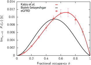
Figure 1: The zero-frequency limit of the power spectrum, $P_{n}(\omega\to 0)=2\sigma^{2}_{n}\tau_{c}$ with $\sigma^{2}_{n}=\overline{n}(1-\overline{n})$, as a function of the average receptor occupancy $\overline{n}$ for $c=0.4\mathrm{\,\mu M}$; $\overline{n}$ is varied by changing $k_{d}$. It is seen thatthe theoretical prediction of Kaizu et al. Kaizu:2014eb (red line) agrees very well with the simulation results (red symbols), in contrast to that of Bialek and Setayeshgar bialek2005 (black line). Parameters: $D=1\mathrm{\,\mu m^{2}\,s^{-1}}$, $\sigma=10\mathrm{\,nm}$, $L=1\mathrm{\,\mu m}$, $k_{a}=552\mathrm{\,\mu M^{-1}s^{-1}}$.

II.5 Role of rebinding

The question remains why the analysis of Kaizu et al. is so accurate. The central assumption of Eq. 11 makes the propensity for binding the next ligand independent of the history of the previous binding events. In essence, it reduces the non-Markovian many-body problem to a Markovian two-body problem, which can be seen from the expression for the receptor correlation time $\tau_{c}=(\sigma^{2}_{n})^{-1}\widehat{C}_{n}(s=0)$:

$$\tau_{c}=\frac{1}{k_{\rm on}c+k_{\rm off}}.$$ (13)

Here $k_{\rm on}$ and $k_{\rm off}$ are the renormalized association and dissociation rates

$$k_{\rm on} =\left(\frac{1}{k_{a}}+\frac{1}{k_{D}}\right)^{-1}=\frac{k_{a}k_{D}}{k_{a}+k_{D}},$$ (14)

$$k_{\rm off} =\left(\frac{1}{k_{d}}+\frac{K_{\rm eq}}{k_{D}}\right)^{-1}=\frac{k_{d}k_{D}}{k_{a}+k_{D}}.$$ (15)

with $K_{\rm eq}=k_{a}/k_{d}=k_{\rm on}/k_{\rm off}$ the equilibrium constant and $k_{D}=4\pi\sigma D$ the diffusion-limited rate constant—$k_{D}=k_{\rm rad}(t\to\infty)$ for $k_{a}\to\infty$. Eq. 13 is the expression for the correlation time of a receptor that switches in a memoryless fashion between the bound and unbound states with switching rates $k_{\rm on}c$ and $k_{\rm off}$.

But why is Eq. 11 accurate? And what is the role of rebindings? Do they not generate an algebraic tail in the correlation function? As it turns out, these questions are intimately related. It is well known that in an unbounded system, the correlation function exhibits an algebraic tail because at long times the relaxation of the receptor state is dominated by the slow diffusive transport of the ligand over long distances Popov2001 ; Gopich2002 . However, we typically expect the space to be bounded, both for the binding of ligand to a receptor inside the cell and to a receptor at the cell surface. Indeed, the simulations of Kaizu:2014eb were performed in a finite box of cellular dimensions, yielding exponential, not algebraic, decay at long times. We then expect Eq. 11 to become accurate. More specifically, assumption Eq. 11 breaks down when a) the rebinding of a dissociated particle is pre-empted by the binding of another particle from the bulk; and b) if this second particle dissociates from the receptor before the first has equilibrated by diffusing into the bulk. However, the time a ligand molecule spends near the receptor is typically much shorter than the time for molecules to arrive from the bulk at biologically relevant concentrations, which means that the probability of rebinding interference is very small, and condition a) is not met. Because biologically relevant concentrations are low, also the dissociation rates are typically low, which means that also condition b) is not met. The likelihood that both conditions are met, necessary for the analysis to break down, is thus very small Kaizu:2014eb .

Because rebindings are so much faster than bulk arrivals, they can be integrated out vanzon2006 ; Kaizu:2014eb ; Mugler:2013wx . The probability that a particle that has just dissociated from the receptor will rebind the receptor rather than diffuse away into the bulk is $p_{\rm reb}=1-S_{\rm rad}(\infty|\sigma)=k_{a}/(k_{a}+k_{D})$. The mean number of rounds of rebinding and dissociation before the molecules diffuse into the bulk is then $N_{\rm reb}=k_{a}/k_{D}$, which rescales the effective dissociation rate: $k_{\rm off}=k_{d}/(N_{\rm reb}+1)=k_{d}k_{D}/(k_{a}+k_{D})$. Similarly, a molecule that arrives at the receptor from the bulk may either bind the receptor or escape back into the bulk with probability $p_{\rm esc}=1-p_{\rm reb}$; the mean number of rounds of escape and arrival before binding is $N_{\rm esc}=1/N_{\rm reb}$, which rescales the effective association rate $k_{\rm on}=k_{D}/(1+N_{\rm esc})=k_{a}k_{D}/(k_{a}+k_{D})$. These are indeed precisely the rates of Eqs. 14 and 15.

This analysis also elucidates the role of rebinding in sensing. The probability of rebinding does not depend on the concentration, and rebindings therefore do not provide information on the concentration. They merely increase the receptor correlation time by increasing the effective receptor on-time from $k_{d}^{-1}$ to $k_{\rm off}^{-1}=k_{d}^{-1}/(1+N_{\rm reb})$. After $(1+N_{\rm reb})$ rounds of dissociation and rebinding, the molecule escapes into the bulk, and then another molecule will arrive at the receptor with rate $k_{D}c$; this molecule may return to the bulk or bind the receptor, such that a new molecule will bind after a time $(k_{\rm on}c)^{-1}$ on average. Importantly, this molecule will bind in a memoryless fashion and with a rate that depends on the concentration. This binding event thus provides an independent concentration measurement. The mean waiting time in between independent binding events is therefore $\tau_{w}=1/k_{\rm off}+1/(k_{\rm on}c)$, which allows us to rewrite Eq. 12 in a form that we would expect intuitively:

$$\left(\frac{\delta c}{c}\right)_{KZ}^{2}=\frac{2}{k_{\rm on}c(1-p)T}=\frac{2\tau_{w}}{T}.$$ (16)

Indeed, the sensing error $\delta c/c$ decreases with the square root of the number of independent measurements $T/\tau_{w}$ during the integration time $T$.

Lastly, why does the expression of Bialek and Setayesghar, Eq. 8, miss the factor $1-p$ in the diffusion term? We believe that this is because by invoking the fluctuation-dissipation theorem, Bialek and Setayesghar effectively linearize the reaction-diffusion problem, thereby ignoring correlations between the state of the receptor and the local ligand concentration. This idea is supported by the analysis of Berezhkovskii and Szabo Berezhkovskii:2013hq , who recently derived an expression for the accuracy of sensing via multiple receptors on a sphere, ignoring spatio-temporal correlations between the states of the respective receptor molecules and the ligand concentration. Interestingly, in the limit that the number of receptors on the sphere goes to infinity, then, by replacing the radius of the cell with the cross section of the receptor, their expression becomes identical to that of Bialek and Setayesghar, see also Eq. 28 below; indeed, this expression does not contain the factor $(1-p)$. This can be understood by noting that in the limit that the number of receptors becomes large, there will always be receptor molecules available for binding the ligand. But for a single receptor, we have to take the binary character of the receptor state into account.

III Can cells reach the Berg-Purcell limit?

The work of Berg and Purcell and subsequent studies like those discussed above berg1977 ; Ueda:2007uq ; bialek2005 ; levinepre2007 ; levineprl2008 ; levineprl2010 ; Skoge:2011gi ; Skoge:2013fq ; Kaizu:2014eb assume not only a given integration time $T$, but also that the downstream signaling network averages the state of the receptor uniformly in time over this integration time $T$. It remained unclear, however, how the signaling network determines the (effective) integration time $T$, whether the network averages the signal uniformly in time, and how this assumption affects the sensing precision Govern2012 . It thus remained open whether signaling networks can actually reach the Berg-Purcell limit.

To address these questions, the authors of Ref. Govern2012 considered linear, but otherwise arbitrary signaling network. For deterministic networks of this type, the output $X(T_{o})$ at time $T_{o}$ can be written as

$$X(t)=\int_{-\infty}^{T_{o}}\chi(T_{o}-t^{\prime})RL(t^{\prime})dt^{\prime},$$ (17)

where $\chi(t-t^{\prime})$ is the response function of the network and $RL(t)$ is the stochastic receptor signal. To compare to previous results, the authors assumed that at $t=0$ the environment changes instantaneously and that the receptors and hence $RL(t)$ immediately adjust, so that $RL(t)$ is stationary for $0<t<T_{o}$, with fluctuations that decay exponentially with correlation time $\tau_{c}$ Kaizu:2014eb . Moreover, they assumed that either: (1) $\chi(T_{o}-t)=0$ for $t<0$, which corresponds to a scenario where the response time $\tau_{r}$ of the network is shorter than $T_{o}$, or, equivalently, the network reaches steady state by the time $T_{o}$; or (2) $RL(t)=0$ for $t<0$, which corresponds to a scenario in which the cell is initially in a basal state. In both cases, $X(t)=\int_{0}^{T_{o}}\chi(T_{o}-t^{\prime})RL(t^{\prime})dt^{\prime}$. When neither $\chi(T_{o}-t)$ nor $RL(t)$ are zero for $t<0$, then previous states of the environment influence the state of the network at $T_{o}$, which can either be a source of noise, or a source of information if the environments are correlated.

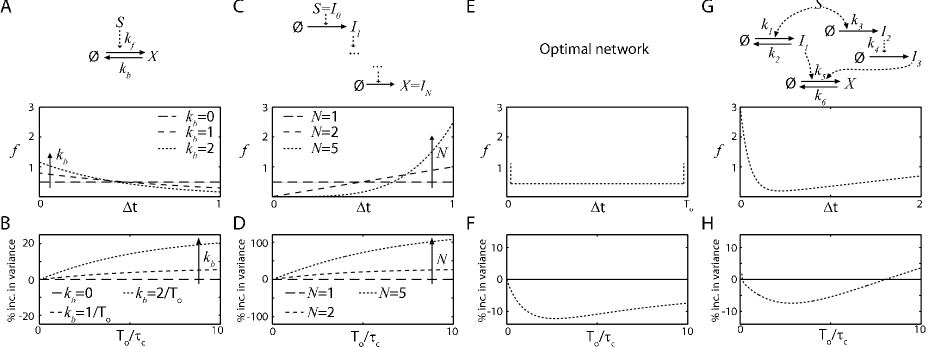
Figure 2: Extracting information from noisy input signals with linear signaling networks. (A,C,E,G) The weighting functions corresponding to different signaling networks are not uniform. (B,D,F,H) The ability of a signaling network to measure ligand concentration depends on its weighting function. The typical error (variance) in the estimate of ligand concentration is plotted as a percentage increase over the error of an estimate based on uniform weighting, assumed in the Berg-Purcell limit (Eq. 1 with $T=T_{o}$). (A) Reversible, one-level cascades selectively amplify late ($t=T_{\rm{o}}$) values of the signal, (B) leading to worse performance than the uniform average. (C) Irreversible, $N$-level cascades amplify early ($t=0$) values of the signal, (D) leading to worse performance than the uniform average. (E) The optimal weighting function, given in Ref. Govern2012 , averages the signal, selectively amplifying less correlated values. The delta functions are truncated for illustration. (F) The optimal weighting function outperforms the uniform average. (G) A signaling network consisting of two branches, which selectively amplify late ($t=T_{\rm{o}}$) (left branch) and early ($t=0$) (right branch) values of the signal, approximates the optimal weighting function ($k_{1}=3.1$; $k_{2}=10$; $k_{3}=1$; $k_{4}=0.35$; $k_{5}=1$; $k_{6}\gg 1$; $T_{\rm{o}}=2$). (H) The network in (F) can outperform the uniform average ($\tau_{\rm c}$ varies for fixed $T_{\rm{o}}=2$).

The idea is that the cell infers the ligand concentration from the output $X(T_{0})$ and by inverting the input-output relation $\overline{X}(c)$. Using error propagation, the error in the estimate of the concentration is then given by

$$\left(\frac{\delta c}{c}\right)_{X}^{2} =\frac{1}{c^{2}}\left(\frac{dc}{d\overline{X}}\right)^{2}\sigma^{2}_{X(T_{0})}.$$ (18)

The authors of Ref. Govern2012 then studied different signaling architectures, shown in Fig. 2. Clearly, these networks do not, in general, average the receptor signal uniformly in time; instead, they have non-uniform weighting functions (Fig. 2A,C,E,G). They weigh receptor signals in the past with a response function that depends on both the lifetime of the signaling molecules and on the topology of the signaling network. One-layer networks consisting of a single reversible reaction give most weight to the most recent signal value (left-most column), while multi-level cascades consisting of irreversible reactions give more weight to signal values more in the distant past (second column). This concept can be generalized to arbitrarily large signaling networks. Multilevel reversible cascades have weighting functions that peak at some finite time in the past, balancing the down-weighting of the signal from the distant past due to the reverse reactions, with the down-weighting of the signal from the recent past resulting from the multilevel character of the network. Linear combinations of the weighting functions for reversible and irreversible cascades can be achieved with multiple cascades that are activated by the input in parallel and which independently activate the same effector molecule. Clearly, signaling networks allow for very diverse weighting functions.

This idea can be exploited to improve the accuracy of sensing, as shown in the right two columns of Fig. 2. A network with a feedforward topology that combines a fast reversible cascade with a slow irreversible cascade cannot only reach the Berg-Purcell limit, but even beat it by $12\%$, when the observation time $T_{o}$ is on the order of the receptor correlation time $\tau_{c}$. The reason is that this network selectively amplifies the more recent signal values and those further back in the past. This is beneficial, because these signal values are less correlated.

While the data processing inequality suggests that it is advantageous to limit the number of nodes in a signaling network to minimize the effect of intrinsic noise, this study shows that there can be a competing effect in favor of increasing the number of nodes: better removal of extrinsic noise. Additional nodes make it possible to sculpt the weighting function for averaging the incoming signal, allowing signaling networks to reach and even exceed the Berg-Purcell limit.

IV Fundamental sensing limit of equilibrium systems

Signaling networks are stochastic in nature, which means that while they may remove the extrinsic noise in the input signal, they will also add their own intrinsic noise to the transmitted signal. Most studies on the accuracy of sensing have ignored this intrinsic noise of the signaling network berg1977 ; Ueda:2007uq ; bialek2005 ; levinepre2007 ; levineprl2008 ; wingreen2009 ; endres2010 ; levineprl2010 ; Govern2012 ; Skoge:2011gi ; Skoge:2013fq ; Kaizu:2014eb ; Lang:2014ir . They essentially assume that the intrinsic noise can be made arbitrarily small and that the extrinsic noise in the receptor signal can be filtered with arbitrary precision by simply integrating the receptor signal for longer. However, the extrinsic and intrinsic noise are not generally independent TanaseNicola2006 . This raises the question whether the extrinsic and intrinsic noise can be lowered simultaneously, and if so, what resources would be required to achieve this.

To address these questions, the authors of Govern:2014ez first studied equilibrium networks that are not driven out of thermodynamic equilibrium via the turnover of fuel. Inspired by one component signaling networks Ulrich:2005ys , they started with the simplest possible equilibrium network, consisting of cytoplasmic readout molecules ${\rm X}$ that directly bind ligand-free receptors ${\rm R}$: ${\rm R}+{\rm L}\rightleftharpoons{\rm RL}$, ${\rm R}+{\rm X}\overset{k_{\rm f}}{\underset{k_{\rm r}}{\rightleftharpoons}}{\rm RX}$. The linearized deviation $\delta x(t)=X(t)-\overline{X}$ of the copy number $X(t)$ from its steady-state value $\overline{X}$ is

$$\delta x(t)=\int_{-\infty}^{t}\chi(t-t^{\prime})\left[\gamma RL(t^{\prime})+\eta(t^{\prime})\right],$$ (19)

where $\chi(t-t^{\prime})=e^{-(t-t^{\prime})/\tau_{I}}$ is the response function with $\tau_{I}=1/(k_{f}(\overline{X}+\overline{R})+k_{r})$ the integration time, $\gamma=k_{\rm f}\overline{X}$, $RL(t)$ is the input signal and $\eta$ describes the intrinsic noise of the signaling network, set by the rate constants and copy numbers.

The sensing error can be computed, as before, via Eq. 18. Here, the variance $\sigma^{2}_{x}=\langle\delta x\rangle^{2}$ can be decomposed into the sum of the extrinsic noise $\sigma_{{\rm ex},x}^{2}\equiv\gamma^{2}K_{\delta RL,\delta RL}$ and the intrinsic noise $\sigma_{{\rm in},x}^{2}\equiv\gamma K_{\delta RL,\eta}+K_{\eta,\eta}$, where $K_{A,B}=\int_{-\infty}^{t}\int_{-\infty}^{t}e^{-(t-t_{1}^{\prime})/\tau_{\rm I}}C_{A,B}(t_{1}^{\prime},t_{2}^{\prime})e^{-(t-t_{2}^{\prime})/\tau_{\rm I}}dt_{1}dt_{2}$ with the correlation function $C_{AB}(t_{1},t_{2})=\langle A(t_{1})B(t_{2})\rangle$. This decomposition is not unique, but in this form the extrinsic noise term features a canonical temporal average of the input (receptor) fluctuations Paulsson:2004dh ; Shibata:2005th ; TanaseNicola2006 , which can be made arbitrarily small by increasing the effective integration time of the network. However, the authors of Ref. Govern:2014ez found that when doing so in a system with $R_{T}$ receptors would reduce the total sensing error below $4/R_{T}$, the intrinsic noise would inevitably rise. The network faces a fundamental trade-off between the removal of extrinsic and intrinsic noise.

Signaling networks are usually far more complicated than one consisting of a single readout species, and as discussed in the previous section, additional network layers can reduce the sensing error Govern2012 . This raises the question whether a more complicated equilibrium network can overcome the limit set by the number of receptors. Searching over all possible network topologies to address this question is impossible. However, equilibrium systems are fundamentally bounded by the laws of equilibrium thermodynamics, regardless of their topology. Indeed, starting from the grand-canonical partition function, one can show that for any equilibrium network the gain $d\overline{X}/d\mu$, with $\mu=\mu^{0}+kT\log(c)$ the chemical potential of the ligand, is given by the co-variance $\sigma^{2}_{X,RL}$ between $X$ and $RL$, because RL (or, in general, the complex containing the ligand) is the species conjugate to the chemical potential. This means that these systems face a trade-off between gain (sensitivity) and noise: increasing the gain inevitably increases the noise. This has marked implications: using $d\overline{X}/d\mu=\sigma^{2}_{X,RL}$ and Eq. 18, we find that the sensing error based on the readout X is $\left(\delta c/c\right)_{X}^{2}=\sigma^{2}_{X}/(\sigma^{2}_{X,RL})^{2}$ , while if the receptors themselves are taken as the readout, the sensing error is $\left(\delta c/c\right)_{RL}^{2}=1/\sigma^{2}_{RL}$. From this it follows that

$$\left(\frac{\delta c}{c}\right)_{X}^{2}=\frac{\sigma_{X}^{2}\sigma_{RL}^{2}}{\left(\sigma_{X,RL}^{2}\right)^{2}}\left(\frac{\delta c}{c}\right)_{RL}^{2}\geq\left(\frac{\delta c}{c}\right)_{RL}^{2}\geq\frac{4}{R_{T}^{2}}.$$ (20)

Here the first equality inequality on the right-hand side follows from the fact that $|\sigma_{X,RL}^{2}|/\sqrt{\sigma_{X}^{2}\sigma_{RL}^{2}}$ is a correlation coefficient, which is always less than 1 in magnitude. The second inequality follows from the observation that for any stochastic variable $0<Y<a$, $\sigma^{2}_{Y}\leq a^{2}/4$, meaning that $\sigma^{2}_{RL}<R_{T}^{2}/4$. Eq. 20 thus shows that in equilibrium systems a downstream signaling network can never improve the accuracy of sensing. The sensing precision is limited by the total number of receptors $R_{T}$, regardless of how complicated the downstream network is, or how many protein copies are devoted to making it.

What is the origin of the sensing limit in equilibrium sensing systems? These systems transduce the signal by harvesting the energy of ligand binding: this energy is used to boot off the downstream signaling molecules from the receptor. However, detailed balance, by putting a constraint on the binding affinities of receptor-readout and receptor-ligand binding, then dictates that receptor-readout binding also influences receptor-ligand binding, thus perturbing the future signal. Indeed, the trade-offs faced by equilibrium networks are all different manifestations of their time-reversibility. The only way for a time-reversible system to “integrate” the past is for it to integrate and hence perturb the future. Concomitantly, in a time reversible system, there is no sense of “upstream” and “downstream”, concepts which rely on a direction of time Feng2008 ; $RL$ is as much a readout of $X$, as the other way around. While in equilibrium systems the readout encodes the receptor state, the readout is not a stable memory that is decoupled from changes in the receptor state: a change in the state of the readout, induced by readout-receptor (un)binding, influences the future receptor state. This introduces cross-correlations between the intrinsic fluctuations in the activation of the readout, modeled by $\eta(t)$ in Eq. 19, and the extrinsic fluctuations in the input $RL(t)$: $K_{RL,\eta}\neq 0$. It is these cross-correlations, which ultimately arise from time reversibility, that lead, in these equilibrium systems, to a fundamental tradeoff between the removal of extrinsic and intrinsic noise and between increasing the gain and suppressing the noise.

V Sensing in non-equilibrium systems

To beat the sensing limit of equilibrium systems, energy and the receptor need to be employed differently. Rather than using the energy of ligand binding to change the state of the readout, the system should use fuel. This makes it possible change the readout via chemical modification, with the receptor catalyzing the modification reaction: ${\rm RL}+{\rm X}\to{\rm RL}+{\rm X}^{*}$. This decouples receptor-ligand binding from receptor-readout binding: the activation of the readout does not influence the future receptor signal, while, conversely, a change in the receptor state does not affect the stability of the readout. Each readout molecule that has interacted with the receptor provides a stable memory; collectively, the readout molecules encode the history of the receptor state. This enables the mechanism of time integration, in which the trade-off between noise and sensitivity is broken, and the extrinsic and intrinsic noise can be reduced simultaneously Govern:2014ez .

Catalysts cannot change the chemical equilibrium of two reactions that are the microscopic reverse of each other. To make the average state of the readout dependent on the average receptor occupancy, the activation reaction ${\rm RL}+{\rm X}\to{\rm RL}+{\rm X}^{*}$ must therefore be coupled to a reaction that is not its microscopic reverse, and the system must be driven out of equilibrium. This is precisely the canonical signaling motif of a receptor driving a push-pull network. In such a network the receptor itself or the enzyme associated with it, like CheA in E. coli chemotaxis, catalyzes the activation of a readout protein X via chemical modification, i.e. the phosphorylation of the messenger protein CheY; active readout molecules ${\rm X}^{*}$ can then decay spontaneously or be deactivated by an enzyme, like the phosphatase CheZ in E. coli, via a reaction that is not the microscopic reverse of the activation reaction. Typically, the activation via chemical modification is coupled to fuel turnover, while deactivation is not; in E. coli chemotaxis, for example, phosphorylation of CheY is fueled by ATP hydrolysis: ${\rm CheA}+{\rm ATP}+{\rm CheY}\to{\rm CheA}+{\rm ADP}+{\rm CheY_{p}}$, while dephosphorylation is not: ${\rm CheZ}+{\rm CheY_{p}}\to{\rm CheZ}+{\rm CheY}+{\rm Pi}$. Another classical example is MAPK signaling, where activation of MAPK is driven by ATP hydrolysis, while deactivation is not (even though it is typically catalyzed by a phosphatase). In all these systems, ATP hydrolysis is used to drive the readout molecule to a high energy state, the active phosphorylated state, which then relaxes back to the inactive dephosphorylated state via another pathway, setting up a cycle in state space leading to energy dissipation.

V.1 The sensing error

To derive the fundamental resources required for sensing, it is instructive to view the downstream system as a device that samples the state of the receptor discretely Govern:2014ef . The activation reaction ${\rm RL}+{\rm X}+{\rm ATP}\overset{k_{\rm f}}{\to}{\rm RL}+{\rm X}^{*}+{\rm ADP}$ (assumed to be fueled by ATP hydrolysis) generates samples of the ligand-binding state of the receptor by storing the receptor state in the stable modification states of the readout molecules. We expect that if there are $N$ receptor-readout interactions, then the cell has $N$ samples of the receptor state and the error in the concentration estimate, $\delta c/c$, is reduced by a factor of $\sqrt{N}$. However, to derive the effective number of samples, we have to consider not only the creation of samples, but also their decay and reliability. The decay reaction ${\rm X}^{*}\overset{k_{\rm r}}{\to}{\rm X}$ is equivalent to discarding or erasing samples. The microscopically reverse reactions of these activation and deactivation reactions, namely the receptor-mediated deactivation ${\rm X^{*}}+{\rm RL}+{\rm ADP}\overset{k_{\rm-f}}{\to}{\rm X}+{\rm RL}+{\rm ATP}$ and the spontaneous (or phosphatase catalyzed) activation ${\rm X}\overset{k_{\rm-r}}{\to}{\rm X}^{*}$ independent of the receptor, generate incorrect samples of the receptor state. Energy is needed to break time-reversibility and to protect the coding.

How the receptor samples are generated, erased, and how they are stored in the readout, determine the number of samples, their independence, and their reliability, which together set the sensing precision Govern:2014ef :

$$\left(\frac{\delta c}{c}\right)^{2}=\frac{1}{p(1-p)}\frac{1}{\bar{N}_{I}}+\frac{1}{(1-p)^{2}}\frac{1}{\bar{N}_{\rm eff}}.$$ (21)

In this expression, obtained using the here accurate linear-noise approximation TanaseNicola2006 ; Govern:2014ef , $p$ is as before the probability that a receptor is bound to ligand. The quantity $\bar{N}_{I}$, discussed below, is the average number of receptor samples that are independent out of a total of $\bar{N}_{\rm eff}$ samples. The first term is the error on the concentration estimate that would be expected on the basis of $\bar{N}_{I}$ perfect, independent samples of the receptor state that can be unambiguously identified (as in Eq. 3). A second correction term arises, however, because the cell cannot distinguish between those readout molecules that have collided with an unbounded receptor since their last dephosphorylation event, and those that have not.

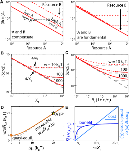
Figure 3: Trade-offs in non-equilibrium sensing. (A) When two resources A and B compensate each other, one resource can always be decreased without affecting the sensing error, by increasing the other resource; concomitantly, increasing a resource will always reduce the sensing error. When both resources are instead fundamental, the sensing error is bounded by the limiting resource and cannot be reduced by increasing the other. (B, C) The three classes time/receptor copies, copies of downstream molecules, and energy are all required for sensing, with no trade-offs among them. The minimum sensing error obtained by minimizing Eq. 21 is plotted for different combinations of (B) $X_{T}$ and $w$, and (C) $R_{T}(1+\tau_{r}/\tau_{c})$ and $w$. The curves track the bound for the limiting resource indicated by the grey lines, showing that the resources do not compensate each other. The plot for the minimum sensing error as a function of $R_{T}(1+\tau_{r}/\tau_{c})$ and $X_{T}$ is identical to that of (C) with $w$ replaced by $X_{T}$. (D) The energy requirements for sensing. In the irreversible regime ($\Delta\mu\to\infty$), the work to take one sample of a ligand-bound receptor, $w/(p\bar{N}_{\rm eff})$, equals $\Delta\mu$, because each sample requires the turnover of one fuel molecule, consuming $\Delta\mu$ of energy. In the quasi-equilibrium regime ($\Delta\mu\to 0$), each effective sample of the bound receptor requires $4{\rm k_{B}T}$, which defines the fundamental lower bound on the energy requirement for taking a sample. When $\Delta\mu=0$, the network is in equilibrium and both $w$ and $\bar{N}$ are $0$. ATP hydrolysis provides $20{\rm k_{B}T}$, showing that phosphorylation of read-out molecules makes it possible to store the receptor state reliably. The results are obtained fromEq. 22 with $\Delta\mu_{1}=\Delta\mu_{2}=\Delta\mu/2$. (E) Sampling more than once per correlation time requires more resources, while the benefit is marginal. As the sampling rate is increased by increasing the readout copy number $X_{T}$, the number of independent measurements $\bar{N}_{I}$ saturates at the Berg-Purcell limit $R_{T}\tau_{r}/\tau_{c}$, but the energy and protein cost ($\propto X_{T}$) continue to rise.

The number of independent measurements $\bar{N}_{I}$ can be expressed in terms of collective variables that describe the resource limitations of the cell

$$\bar{N}_{I}=\underbrace{\frac{1}{(1+2\tau_{c}/\Delta)}}_{f_{I}}\underbrace{\overbrace{\frac{\left(e^{\Delta\mu_{1}}-1\right)\left(e^{\Delta\mu_{2}}-1\right)}{e^{\Delta\mu}-1}}^{q}\overbrace{\frac{\dot{n}\tau_{r}}{p}}^{\bar{N}}}_{\bar{N}_{\rm eff}}.$$ (22)

This expression has a clear interpretation. The relaxation time $\tau_{r}$ is the effective integration time. The quantity $\dot{n}$ is the flux of X across the cycle of activation by the receptor and deactivation. The product $\dot{n}\tau_{r}$ is thus the number of cycles of read-out molecules involving collisions with ligand-bound receptor molecules during the integration time $\tau_{r}$. The quantity $\dot{n}\tau_{r}/p$ is the total number of read-out cycles involving collisions with receptor molecules, be they ligand bound or not. It is thus the total number of receptor samples taken during $\tau_{r}$, $\bar{N}$.

Not all of these samples are reliable. The effective number of samples taken during $\tau_{r}$ is $\bar{N}_{\rm eff}=q\bar{N}$, where $0\leq q\leq 1$ measures the quality of each sample. Here, $\Delta\mu_{1}$ and $\Delta\mu_{2}$ are the average free-energy drops across the activation and deactivation pathway respectively, in units of ${\rm k_{B}T}$; $\Delta\mu=\Delta\mu_{1}+\Delta\mu_{2}$ is the total free-energy drop across the cycle, which is given by the free energy of the fuel turnover, such as that of ATP hydrolysis. When $\Delta\mu=\Delta\mu_{1}=\Delta\mu_{2}=0$, an active read-out molecule is as likely to be created by the ligand-bound receptor as it is created spontaneously and there is no coding and no sensing; indeed, in this limit, $q=0$ and $\bar{N}_{\rm eff}=0$. In contrast, when $\Delta\mu_{1},\Delta\mu_{2}\to\infty$, $q\to 1$ and $\bar{N}_{\rm eff}\to\bar{N}$.

The factor $f_{I}$ denotes the fraction of samples that are independent. It depends on the correlation time $\tau_{c}$ of receptor-ligand binding and on the time interval $\Delta=2\tau_{r}/(\bar{N}_{\rm eff}/R_{T})$ between samples of the same receptor. Samples farther apart are more independent.

V.2 Fundamental resources and trade-offs

Eqs. 21 and 22 can be used to find the resources that fundamentally limit sensing. A fundamental resource or combination of resources is a (collective) variable that when fixed, puts a lower bound on the sensing error, no matter how the other variables are varied. It can be find via constraint-based optimization, yielding Govern:2014ef :

$$\left(\frac{\delta c}{c}\right)^{2}\geq{\rm MAX}\left(\frac{4}{R_{T}\tau_{r}/\tau_{c}},\frac{4}{X_{T}},\frac{4}{\dot{w}\tau_{r}}\right).$$ (23)

This expression identifies three fundamental resource classes, each yielding a fundamental sensing limit: $R_{T}(1+\tau_{r}/\tau_{c})$, which for the relevant regime of time integration $\tau_{r}>\tau_{c}$ is $R_{T}\tau_{r}/\tau_{c}$, $X_{T}$, and $\dot{w}\tau_{r}$. These classes cannot compensate each other in achieving a desired sensing precision, and hence do not trade-off against each other. The sensing precision is, like the weakest link in a chain, bounded by the limiting resource, as illustrated in Fig. 3A-C. However, within each class, trade-offs are possible. We now briefly discuss the fundamental resource classes and their associated sensing limits.

Receptors and their integration time, $R_{T}\tau_{r}/\tau_{c}$. The number of receptor samples increases with the number of readout molecules, $X_{T}$. In fact, as $X_{T}\to\infty$, the spacing between the samples $\Delta\to 0$ and the effective number of receptor samples $\overline{N}_{\rm eff}\to\infty$; this is indeed the Berg-Purcell mechanism of time integration. However, each receptor can take an independent concentration measurement only every $2\tau_{c}$, meaning that the number of independent measurements taken during the integration time $\tau_{r}$ is, per receptor, $\tau_{r}/\tau_{c}$ (the disappearance of the factor 2 is due to the fact that the deactivation of X increases the effective spacing between the samples, see Govern:2014ef ). Assuming that the receptors bind independently (but see section VI.2), the total number of independent concentration measurements, $\overline{N}_{I}$, taken during $\tau_{r}$, is then limited by $R_{T}\tau_{r}/\tau_{c}$, no matter how large $X_{T}$ is (Fig. 3E). This yields the sensing limit of Berg and Purcell, $\left(\delta c/c\right)^{2}\geq 4/(R_{T}\tau_{r}/\tau_{c})$, recognizing that the receptors are assumed to bind independently, and $p(1-p)\leq 0.25$ (cf. Eq. 3). While the product $R_{T}\tau_{r}/\tau_{c}$ is fundamental, $R_{T}$ and $\tau_{r}$ are not: the error is determined by the total number of independent concentration measurements, and it does not matter whether these measurements are performed by many receptors over a short integration time or by one receptor over a long integration time.

The number of readout molecules, $X_{T}$. Each concentration measurement needs to be stored in the chemical modification state of a readout molecule, and $X_{T}$ limits the maximum number of measurements that can be stored. Consequently, no matter how many receptors the cell has, or how much time it uses to integrate the receptor state, the sensing error is fundamentally limited by the pool of readout molecules, $\left(\delta c/c\right)^{2}\geq 4/X_{T}$.

Energy, $\dot{w}\tau_{r}$, during the integration time. The power, the rate at which the fuel molecules do work, is $\dot{w}=\dot{n}\Delta\mu$, and the total work performed during the integration time is $w\equiv\dot{w}\tau_{r}$. This work is spent on taking samples of receptor molecules that are bound to ligand, because only they can modify $X$. The total number of effective samples of ligand-bound receptors obtained during $\tau_{r}$, is $p\overline{N}_{\rm eff}$. Hence, the work needed to take one effective sample of a ligand-bound receptor is $w/(p\bar{N}_{\rm eff})=\Delta\mu/q$ (see Eq. 22). Fig. 3D shows this quantity as a function of $\Delta\mu$. In the limit that $\Delta\mu\gg 4k_{B}T$, $w/(p\bar{N}_{\rm eff})=\Delta\mu$, because the quality factor $q\to 1$; in this regime, each receptor state is reliably encoded in the chemical modification state of the readout, and increasing $\Delta\mu$ further increases increases the sampling cost with no reward in accuracy. In the opposite regime, $\Delta\mu<4k_{B}T$, however, the quality of the samples, $q$, rapidly decreases with decreasing $\Delta\mu$. In this regime, the system must take multiple noisy receptor samples to give the same information as one single perfect sample. In the limit $\Delta\mu\to 0$, the quality factor $q\to\Delta\mu/4$ and the work to take one effective sample of a ligand-bound receptor approaches its minimal value of $w/(p\overline{N}_{\rm eff})=\Delta\mu/q=4kT$. Substituting this in Eq. 21 yields another bound on the sensing error: $\left(\delta c/c\right)^{2}\geq 4/(\dot{w}\tau_{r})$. The bound can be reached when $R_{T}\tau_{r}/\tau_{c}$ and $X_{T}$ are not limiting, and $\Delta\mu\to 0$. This bound shows that while the total work $w=\dot{w}\tau_{r}$ done during the integration time $\tau_{r}$ is fundamental, the power $\dot{w}$ and $\tau_{r}$ are not, leading to a trade-off between accuracy, speed and power, as found in adaptation Tu2012 .

V.3 Design principle of optimal resource allocation

The observation that resources cannot compensate each other, naturally yields the design principle of optimal resource allocation, which states that in an optimally designed system, each resource is equally limiting so that no resource is in excess and thus wasted. Quantitatively, Eq. 23 predicts that in an optimally designed system

$$R_{T}\tau_{r}/\tau_{c}\approx X_{T}\approx w.$$ (24)

In an optimal sensing system, the number of independent concentration measurements $R_{T}\tau_{r}/\tau_{c}$ equals the number of readout molecules $X_{T}$ that store these measurements and equals the work (in units of $k_{B}T$) to create the samples. Interestingly, the authors of Ref. Govern:2014ef found that the chemotaxis system of E. coli obeys the principle of optimal resource allocation, Eq. 24. This indicates that there is a selective pressure on the optimal allocation of resources in cellular sensing.

VI Discussion

VI.1 Different sensing strategies encode and decode ligand information differently

Cells use different sensing strategies, which differ in how they process information about the ligand concentration. The data processing inequality Cover2012 guarantees for any network that no readout $X$ can have more information about the ligand concentration encoded in its time trace than the ligand-bound receptor $RL$ has in its time-trace Govern:2014ez : $I(X_{[0,T]}(t);\mu_{L})\leq I(RL_{[0,T]}(t);\mu_{L})$, where $I$ is the mutual information between the arguments with $\mu_{L}$ the chemical potential of the ligand, and $y_{[0,T]}(t)$ indicates the time trace of $y=X,RL$ from time 0 to time $T$. Clearly, the accuracy of sensing for any network is bounded by the amount of information that is in the time trace of the receptor state. However, the different sensing strategies differ in how they encode the ligand concentration in the receptor dynamics and in how they decode the information that is in the receptor time trace.

For equilibrium networks, the data processing inequality guarantees that no readout has more information about the ligand than the receptors at any given time Govern:2014ez : $I(X(T);\mu_{L})\leq I(RL(T);\mu_{L})\leq\log_{2}(R_{\rm T}+1)$, and therefore the information in the instantaneous level of the readout is bounded by the total number of receptors $R_{T}$. This statement is the information-theoretic analogue of Eq. 20. The history of receptor states does contain more information about the ligand concentration than the instantaneous receptor state, but an equilibrium signaling network cannot exploit this: its output contains no more information than the instantaneous receptor state.

Cells that use the mechanism of time integration can exploit the information that is the time trace of the receptor, and for these networks $I(X(T);\mu_{L})$ can be larger than $I(RL(T);\mu_{L})$. These cells estimate the ligand concentration from the average receptor occupancy over an integration time, which, as we have seen in section III, is determined by the architecture of the readout system and the lifetime of the readout molecules. It is quite clear that cells employ this mechanism of time integration: the central motif of cell signaling in both prokaryotes and eukaryotes, the push-pull network, implements time averaging by storing the receptor state into stable chemical modification states of the readout molecules, which, collectively, encode the average receptor occupancy over the past integration time.

Another sensing strategy is maximum likelihood estimation wingreen2009 ; mora2010 ; Lang:2014ir . It estimates the ligand concentration not from the average receptor occupancy over the integration time $T$, as in the mechanism of time integration, but rather from the mean duration of the unbound state of the receptor $\tau_{u}$: $\hat{c}_{\rm MLE}=1/(\tau_{u}k_{\rm on})$. The sensing error of this strategy for a single receptor is $\left(\delta c/c\right)^{2}_{\rm MLE}=1/(k_{\rm on}c(1-p)T)$ wingreen2009 , which is half that of the mechanism of time integration, see Eq. 16. The reason why this sensing strategy is more accurate is that only the binding rate depends on the concentration, not the unbinding rate. Hence, only the unbound interval provides information on the concentration. In contrast, the mechanism of time integration infers the concentration from the mean receptor occupancy, which depends on both the unbound interval and the uninformative bound interval.

How cells could actually implement the strategy of maximum-likelihood estimation remains an open question. One possibility is that receptors are internalized upon ligand binding, another that they bind ligand only briefly and signal only transiently, which could be achieved via receptor adaptation or desensitization following ligand binding wingreen2009 . Another intriguing possibility has recently been suggested by Lang et al. Lang:2014ir . It is inspired by the observation that many receptors, such as receptor-tyrosine kinases and G-protein coupled receptors, are chemically modified via fuel turnover Lang:2014ir . In this scheme, the cell estimates the ligand concentration from the average receptor occupancy over an integration time $T$, as in the canonical mechanism of time integration. However, upon ligand binding, the receptor is driven via fuel turnover through a non-equilibrium cycle of $m$ chemical modification steps, before it can release and bind new ligand again. In the limit that the energy drop over the cycle $\Delta\mu\to\infty$ and $m\to\infty$, the sensing accuracy approaches the maximum-likelihood-estimation limit, even though the concentration is inferred from the average receptor occupancy. The reason is that in this limit the interval distribution of the active receptor state becomes a delta function instead of an exponential one as in the case of canonical time integration. This eliminates the noise from the uninformative bound interval in estimating the average receptor occupancy.

VI.2 The importance of spatio-temporal correlations

Ultimately, the precision of sensing via a mechanism that relies on integrating the receptor state, be it the canonical Berg-Purcell scheme with Markovian active receptor states or the maximum-likelihood scheme of Lang et al. with non-Markovian active states Lang:2014ir , is determined by the number of receptors, the receptor correlation time, and how the readout molecules sample the receptor molecules. The analysis of Ref. Govern:2014ef ignores any spatio-temporal correlations of both the ligand molecules and the readout molecules. In this analysis, the different receptor molecules bind the ligand molecules independently, and the correlation time of the receptor cluster is that of a single receptor molecule $\tau_{c}$. The total number of independent concentration measurements in the integration time $T$ is then the number of receptors $R_{T}$ times the number of independent measurements per receptor, $T/\tau_{c}$, yielding the fundamental limit $\left(\delta c/c\right)^{2}\geq 2\tau_{c}/(p(1-p)R_{T}T)$. Importantly, because $\tau_{c}$ is independent of the number of receptors, the sensing error decreases with the number of receptors. However, diffusion introduces spatio-temporal correlations between the different ligand-receptor binding events berg1977 ; bialek2005 ; levinepre2007 ; Berezhkovskii:2013hq . Consequently, the correlation time $\tau_{N}$ of $R_{T}$ receptors on a spherical cell of radius ${\cal R}$ is not that of a single receptor molecule, but is rather given by Berezhkovskii:2013hq

$$\tau_{N}=\frac{1}{k_{a}c+k_{d}}+\frac{k_{a}\left(k_{a}c+R_{T}k_{d}\right)}{4\pi D{\cal R}\left(k_{a}c+k_{d}\right)^{2}}.$$ (25)

As pointed out by Wang et al. levinepre2007 , the correlation time $\tau_{N}$ increases with the number of receptors $R_{T}$ (and even diverges for $R_{T}\to\infty$), which means that when $R_{T}$ is large and/or the integration time $T$ is short, the mechanism of time integration breaks down. In this regime the equilibrium sensing strategy is superior, because it relies on sensing the instantaneous receptor state levinepre2007 . Using receptors that bind ligand non-cooperatively as the readout, $\left(\delta c/c\right)^{2}_{RL}=1/\sigma^{2}_{RL}=1/((p(1-p)R_{T})$, which indeed decreases with $R_{T}$ levinepre2007 ; Govern:2014ez .

When the integration time $T$ is longer than $\tau_{N}$, the sensing error is given by Berezhkovskii:2013hq

$$\left(\frac{\delta c}{c}\right)^{2} =\frac{2\tau_{N}}{R_{T}Tp(1-p)}$$ (26)

$$=\frac{2}{R_{T}k_{a}cT}\left(1+\frac{k_{a}c}{k_{d}}\right)+\frac{1}{2\pi D{\cal R}cT}\left(1+\frac{k_{a}c}{R_{T}k_{d}}\right).$$ (27)

For large $R_{T}$ (but not so large that $\tau_{N}>T$), the sensing error reduces to

$$\left(\frac{\delta c}{c}\right)^{2} =\frac{1}{2\pi D{\cal R}cT}.$$ (28)

This, apart from the factor $1-p$, is the classical result of Berg and Purcell berg1977 ; bialek2005 . At sufficiently large $R_{T}$, the sensing error is limited by diffusion, the size of the cell and the integration time. It becomes independent of $R_{T}$, because the decrease of the instantaneous error with $R_{T}$, $1/(R_{T}(p(1-p))$, is cancelled by the increase of the correlation time with $R_{T}$.

Not only in the encoding of the ligand concentration in the receptor dynamics, but also in the decoding of this information by the readout system, spatio-temporal correlations can become important. Receptor and readout molecules are often spatially partitioned, due e.g., to the underlying cytoskeletal network or lipid rafts. Even in a system that is spatially homogeneous on average, spatio-temporal partitioning would occur, because of the finite speed of diffusion. We have recently shown that this partitioning decreases the propagation of noise, essentially because the activation of the different readout molecules becomes less correlated Mugler:2013bx . Whether there exists an optimal diffusion constant of the readout molecules that matches the correlation length and time of the receptors, which is set by the ligand diffusion and binding dynamics, is an intriguing question for future work.

VI.3 Cooperative receptor activation

One important aspect that we have not addressed so far is the role of receptor cooperativity. It is now well established that receptors are often activated cooperatively, with the most studied and best characterized example being the receptor cluster of the E. coli chemotaxis system. How does this affect the precision of sensing? This depends (again) on the receptor correlation time Skoge:2013fq . Skoge et al. found that while cooperative interactions between neighboring receptors can increase the gain, which reduces the sensing error, they also increase the correlation time, such that independent receptors are, in fact, optimal. As we now know, equilibrium systems do not rely on time integration, and hence do not suffer from a slowing down of the receptor dynamics. In fact, we have shown that for all equilibrium systems in which the receptors bind the ligand non-cooperatively, $\left(\delta c/c\right)_{X}^{2}\geq 1/R_{T}$; hence, to reach the bound of Eq. 20 for all equilibrium networks, cooperative ligand binding is necessary Govern:2014ez . In Govern:2014ez we show that cooperative ligand binding makes it indeed possible to beat the non-cooperative bound, but whether equilibrium sensing systems can actually reach the bound of Eq. 20 remains an open question.

VI.4 The role of energy in sensing

It seems intuitively clear that fuel turnover can be used to enhance the precision of sensing, but how it can be used is less obvious. In the maximum-likelihood scheme of Lang et al. it is used to make the interval-distribution of the active receptor state more deterministic Lang:2014ir . In the scheme of time integration, fuel turnover is used to sample the receptor state Mehta2012 ; Govern:2014ef .

The latter example seems tantalisingly related to the thermodynamics of computation, formulated by Bennett and Landauer decades ago Bennett:1982hi ; Landauer1961 . In particular, the receptor state appears to be copied into the chemical modification states of readout molecules, which thereby acts as memory elements for time integration Mehta2012 ; Govern:2014ef . Performing copy operations repeatedly using the same readout requires net work input, unless the correlation between the data bit (receptor) and the memory (readout), generated by the copy operation, is used to extract work Ouldridge:2015vi . Indeed, the arguments of Landauer and Bennett Bennett:1982hi ; Landauer1961 show that the minimal amount of work for a perfect copy cycle is $k_{B}T\ln(2)$. But how does this bound apply to biochemical networks?

To answer this question it is important to make a formal mapping between cellular sensing systems and copy operations. As it turns out, cellular copy protocols differ fundamentally from ideal quasi-static protocols, such as those considered by Landauer and Bennett Bennett:1982hi ; Landauer1961 . Copying entails changing the state of the memory, which means that a thermodynamic driving force must be applied to the system. Thermodynamically optimal protocols increase the driving force slowly, such that the memory is slowly driven to its new state. In contrast, in cellular systems the thermodynamic driving force for the reactions that implement the copy process is typically constant, because the fuel molecules that drive these reactions are commonly present at constant concentration Ouldridge:2015vi . As a result, cellular systems face a trade-off between cost and precision that is both qualitatively and quantitatively distinct from that required thermodynamically, regardless of parameters Ouldridge:2015vi . They dissipate more to achieve the same accuracy. One of the most vivid manifestations of this difference concerns the Landauer limit itself. One of the surprising, but by now well-known, results of Bennett and Landauer was that quasi-static protocols make it possible to perform repeated copies with 100% accuracy at only a finite energy cost of, indeed, $k_{B}T\ln(2)$ per copy. In contrast, cellular copy protocols can only reach 100% accuracy when the cost diverges. For the purpose of sampling a noisy signal, however, perfect copies are not necessarily ideal. Indeed, as we have seen in section V.2, the energetically most efficient approach to record the receptor state is to take many noisy samples, which together make up one effective sample. For the canonical push-pull network considered here the minimal cost to take one effective receptor sample is $2k_{B}T$ on average if the receptor occupancy is $p=0.5$ Govern:2014ef . For a bi-functional kinase system, in which the kinase associated with the receptor catalyzes the phosphorylation of the readout when the receptor is bound to ligand, but dephosphorylation when the receptor is not bound to ligand, this minimal cost is even lower: $1k_{B}T$ Ouldridge:2015vi .

VI.5 How resources determine the fundamental sensing limit: Trade-offs between equilibrium and non-equilibrium sensing

Information processing devices require resources to be built and run. Components are needed to construct the system, space is required to accommodate the components and energy is required to make the components and operate the system. These resources constrain the design and performance of any device, and cellular sensing systems are no exception. Making proteins is costly Dekel2005 . They also take up valuable space: both the membrane and the cytoplasm are highly crowded, with proteins occupying 25–75% of the membrane area Linden2012 and 20–30% of the cytoplasmic volume Ellis2001 . And many cellular signaling pathways, including two-component systems in bacteria Stock:2000ve , GTP-ase cycles as in the Ras system Pylayeva-Gupta:2011kx , phosphorylation cycles as in MAPK cascades Chang:2001uq , are driven out of thermal equilibrium via the turnover of fuel. Also the adaptation system that allows E. coli to adapt to a wide range of background concentrations is driven out of equilibrium Tu2012 . However, cells also commonly employ equilibrium motifs, such as protein binding and sequestration. Indeed, as we have seen, sensing does not fundamentally require energy input Govern:2014ez . Equilibrium sensing systems can respond to changes in the environment by harvesting the energy of ligand binding, thereby capitalizing on the work that is performed by the environment to change the ligand concentration. Also adaptation does not fundamentally require energy consumption Endres .

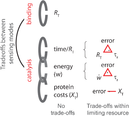
Figure 4: Cells face a fundamental trade-off between two modes of sensing, an equilibrium mode based on binding and sequestration and a non-equilibrium mode based on catalysis. These sensing strategies have different resource requirements.

When does the non-equilibrium sensing strategy outperform the equilibrium one? This depends on the resources available to the cell, as summarized in Fig. 4. Comparing the bound for non-equilibrium systems, Eq. 23, with that for equilibrium ones without cooperative binding, $\left(\delta c/c\right)^{2}\geq 1/R_{T}$, predicts that non-equilibrium systems can sense more accurately when there is at least one readout molecule available per receptor, and the amount of energy dissipated per receptor during the integration time is at least $1k_{B}T$ Govern:2014ez .

Interestingly, evolution may have toggled between equilibrium and non-equilibrium sensing strategies. Bacteria employ both one- and two-component signaling networks. One-component systems follow the equilibrium strategy, consisting of adaptor proteins which can bind an upstream ligand and a downstream effector. Two-component systems are similar to the non-equilibrium push-pull system considered here, consisting of a kinase (receptor) and its substrate. Intriguingly, some adaptor proteins, like RocR, contain the same-ligand binding domain as the kinase and the same effector-binding domain as the substrate of a two-component system, i.e. NtrB-NtrC Ulrich:2005ys . They could thus transmit the same signal. Our results suggest that these are alternative signaling strategies, selected because of different resource selection pressures. It is tempting to believe that when sensing precision is important, but space for receptors on the membrane is limiting, non-equilibrium sensing becomes essential, because it makes it possible to take more concentration measurements per receptor.

VII Conclusion

In this review we have focused on sensing concentrations that do not vary on the timescale of the response of the system. While some questions remain open, such as the importance of spatio-temporal correlations in both ligand-receptor and receptor-readout binding, this problem is by now fairly well understood. We understand how the receptor correlation time depends on the diffusion and binding kinetics of the ligand (although the question of the correlation time of multiple receptors is, arguably, still open), how the effective integration time depends on the lifetime of the readout molecules and the architecture of the readout network, and how the precision of sensing depends on the number of receptors, the number of readout molecules, the receptor correlation time, the integration time, and energy. We understand how combinations of resources impose fundamental sensing limits and what this implies for the optimal design of cellular sensing systems.

The challenge will be to make a similar leap for systems that do not respond rapidly on the timescale of variations in the input signal. For these systems, we have to take the dynamics of the input signal into account. On this front, progress has been made in recent years. We are now beginning to understand how in these systems information transmission depends on the lifetime of the readout molecules and on the topology of the readout network tostevin2010 ; deRonde:2010hh ; deRonde:2012fs ; Aquino:2014co , and what the trade-off between energy dissipation and information processing is Barato2013 ; Barato:2014ta ; Horowitz:2014wb ; Sartori:2014gz . Yet, many questions are still wide open: What is the performance measure that best descibres the design logic of cellular sensing systems? Is it the average sensing error, the instantaneous mutual information, the information transmission rate tostevin2010 , or the learning rate Barato:2014ta ; Horowitz:2014wb ? What resource combinations impose fundamental sensing limits? Also new questions arise: How accurately can living cells predict the future input signal Becker:2013uk ? And what are the thermodynamic costs of cellular prediction Still:2012df ; Becker:2013uk ? The physics of sensing will remain a fascinating problem for many years to come.

VIII Acknowledgements

This work is part of the research programme of the Foundation for Fundamental Research on Matter (FOM), which is part of the Netherlands Organisation for Scientific Research (NWO).

References

- (1) F. Rieke and D. Baylor, Reviews of Modern Physics 70, 1027 (1998).
- (2) J. Boeckh, K.-E. Kaissling, and D. Schneider, Cold Spring Harbor Symp. Quant. Biol 30, 1263 (1965).
- (3) H. C. Berg and E. M. Purcell, Biophysical Journal 20, 193 (1977).
- (4) V. Sourjik and H. C. Berg, Proceedings of the National Academy of Sciences USA 99, 123 (2002).
- (5) M. Ueda and T. Shibata, Biophysical Journal 93, 11 (2007).
- (6) T. Gregor, D. W. Tank, E. F. Wieschaus, and W. Bialek, Cell 130, 153 (2007).
- (7) T. Erdmann, M. Howard, and P. R. ten Wolde, Physical Review Letters 103, 2 (2009).
- (8) J. O. Dubuis et al., Proceedings of the National Academy of Sciences of the United States of America 110, 16301 (2013).
- (9) W. Bialek and S. Setayeshgar, Proceedings of the National Academy of Sciences USA 102, 10040 (2005).
- (10) K. Wang, W.-J. Rappel, R. Kerr, and H. Levine, Physical Review E 75, 061905 (2007).
- (11) W.-J. Rappel and H. Levine, Physical Review Letters 100, 228101 (2008).
- (12) R. G. Endres and N. S. Wingreen, Physical Review Letters 103, 158101 (2009).
- (13) B. Hu, W. Chen, W.-J. Rappel, and H. Levine, Physical Review Letters 105, 048104 (2010).
- (14) T. Mora and N. S. Wingreen, Physical Review Letters 104, 248101 (2010).
- (15) C. C. Govern and P. R. ten Wolde, Physical Review Letters 109, 218103 (2012).
- (16) P. Mehta and D. J. Schwab, Proceedings of the National Academy of Sciences USA 109, 17978 (2012).
- (17) M. Skoge, Y. Meir, and N. S. Wingreen, Physical Review Letters 107, 178101 (2011).
- (18) M. Skoge, S. Naqvi, Y. Meir, and N. S. Wingreen, Physical Review Letters 110, 248102 (2013).
- (19) K. Kaizu et al., Biophysical journal 106, 976 (2014).
- (20) C. C. Govern and P. R. ten Wolde, Proceedings of the National Academy of Sciences of the United States of America 111, 17486 (2014).
- (21) C. C. Govern and P. R. ten Wolde, Physical Review Letters 113, 258102 (2014).
- (22) A. H. Lang, C. K. Fisher, T. Mora, and P. Mehta, Physical Review Letters 113, 148103 (2014).
- (23) G. Aquino and R. G. Endres, Physical Review E 81, 021909 (2010).
- (24) A. M. Berezhkovskii and A. Szabo, The Journal of Chemical Physics 139, 121910 (2013).
- (25) C. H. Bennett, International Journal of Theoretical Physics 21, 905 (1982).
- (26) R. Landauer, IBM Journal of Research and Development 5, 183 (1961).
- (27) T. E. Ouldridge, C. C. Govern, and P. R. Wolde, arXiv.org (2015).
- (28) J. Paijmans and P. R. ten Wolde, Physical Review E 90, 032708 (2014).
- (29) D. Chandler, J. Chem. Phys. 68, 2959 (1978).
- (30) N. B. Becker and P. Rein ten Wolde, The Journal of Chemical Physics 136, 174119 (2012).
- (31) N. Agmon and A. Szabo, The Journal of Chemical Physics 92, 5270 (1990).
- (32) S. A. Rice, in Diffusion-limited reactions, edited by C. Bamford, C. Tipper, and R. Compton (Elsevier, Amsterdam, 1985).
- (33) J. S. van Zon and P. R. ten Wolde, Physical Review Letters 94, 1 (2005).
- (34) J. S. van Zon and P. R. ten Wolde, The Journal of chemical physics 123, 234910 (2005).
- (35) K. Takahashi, S. Tănase-Nicola, and P. R. ten Wolde, Proceedings of the National Academy of Sciences of the United States of America 107, 2473 (2010).
- (36) A. V. Popov and N. Agmon, The Journal of Chemical Physics 115, 8921 (2001).
- (37) I. V. Gopich and A. Szabo, The Journal of Chemical Physics 117, 507 (2002).
- (38) J. S. van Zon, M. J. Morelli, S. Tanase-Nicola, and P. R. ten Wolde, Biophysical Journal 91, 4350 (2006).
- (39) A. Mugler and P. R. ten Wolde, Advances in Chemical Physics 153, 373 (2013).
- (40) S. Tănase-Nicola, P. B. Warren, and P. R. Ten Wolde, Physical Review Letters 97, 068102 (2006).
- (41) L. E. Ulrich, E. V. Koonin, and I. B. Zhulin, Trends in Microbiology 13, 52 (2005).
- (42) J. Paulsson, Nature 427, 415 (2004).
- (43) T. Shibata and K. Fujimoto, Proceedings of the National Academy of Sciences 102, 331 (2005).
- (44) E. H. Feng and G. E. Crooks, Physical Review Letters 101, 090602 (2008).
- (45) G. Lan et al., Nature Physics 8, 422 (2012).
- (46) T. M. Cover and J. A. Thomas, Elements of Information Theory (John Wiley and Sons, Hoboken, New Jersey, 2012).
- (47) A. Mugler, F. Tostevin, and P. R. ten Wolde, Proceedings of the National Academy of Sciences of the United States of America 110, 5927 (2013).
- (48) E. Dekel and U. Alon, Nature 436, 588 (2005).
- (49) M. Lindén, P. Sens, and R. Phillips, PLoS Computational Biology 8, e1002431 (2012).
- (50) R. J. Ellis, Current Opinion in Structural Biology 11, 114 (2001).
- (51) A. M. Stock, V. L. Robinson, and P. N. Goudreau, Annual Review of Biochemistry 69, 183 (2000).
- (52) Y. Pylayeva-Gupta, E. Grabocka, and D. Bar-Sagi, Nature Reviews Cancer 11, 761 (2011).
- (53) L. Chang and M. Karin, Nature 410, 37 (2001).
- (54) G. De Palo and R. G. Endres, PLoS Computational Biology 9, e1003300 (2013).
- (55) F. Tostevin and P. R. ten Wolde, Physical Review Letters 102, 218101 (2009).
- (56) W. de Ronde, F. Tostevin, and P. R. ten Wolde, Physical Review E 82, 031914 (2010).
- (57) W. de Ronde, F. Tostevin, and P. ten Wolde, Physical Review E 86, 021913 (2012).
- (58) G. Aquino, L. Tweedy, D. Heinrich, and R. G. Endres, Scientific reports 4, (2014).
- (59) A. Barato, D. Hartich, and U. Seifert, Physical Review E 87, 042104 (2013).
- (60) A. C. Barato, D. Hartich, and U. Seifert, New Journal of Physics (2014).
- (61) J. M. Horowitz and M. Esposito, Physical Review X (2014).
- (62) P. Sartori, L. Granger, C. F. Lee, and J. M. Horowitz, PLoS Computational Biology 10, e1003974 (2014).
- (63) N. B. Becker, A. Mugler, and P. R. Wolde, arXiv.org (2013).
- (64) S. Still, D. Sivak, A. Bell, and G. Crooks, Physical Review Letters 109, 120604 (2012).