Energy Efficiency of Downlink Networks with Caching at Base Stations

Abstract

Caching popular contents at base stations (BSs) can reduce the backhaul cost and improve the network throughput. Yet whether locally caching at the BSs can improve the energy efficiency (EE), a major goal for 5th generation cellular networks, remains unclear. Due to the entangled impact of various factors on EE such as interference level, backhaul capacity, BS density, power consumption parameters, BS sleeping, content popularity and cache capacity, another important question is what are the key factors that contribute more to the EE gain from caching. In this paper, we attempt to explore the potential of EE of the cache-enabled wireless access networks and identify the key factors. By deriving closed-form expression of the approximated EE, we provide the condition when the EE can benefit from caching, find the optimal cache capacity that maximizes the network EE, and analyze the maximal EE gain brought by caching. We show that caching at the BSs can improve the network EE when power efficient cache hardware is used. When local caching has EE gain over not caching, caching more contents at the BSs may not provide higher EE. Numerical and simulation results show that the caching EE gain is large when the backhaul capacity is stringent, interference level is low, content popularity is skewed, and when caching at pico BSs instead of macro BSs.

I Introduction

To meet the explosive demands for throughput, support sustainable development and reduce global carbon dioxide emission, energy efficiency (EE) has become a major performance metric for 5th generation (5G) cellular networks. While EE of a network can be improved from various aspects such as introducing new network architecture [2], optimizing network deployment and resource allocation [3, 4], an alternative approach is rethinking the goal of the network. Recently, it has been observed that a large portion of mobile multimedia traffic is generated by many duplicate downloads of a few popular contents [5, 6]. This reflects a shift in major goal of the networks from traditional transmitter-receiver communication to content dissemination. On the other hand, the storage capacity of today’s memory devices grows rapidly. As a consequence, equipping caches at base stations (BSs) offers a promising way to unleash the potential of cellular networks except continuing densifying the networks [7, 8].

Caching is a technique to improve performance well known in many wired network domains, e.g., content-centric networks (CCN) [9, 10, 11]. In cellular networks, caching popular contents in the edge can reduce the backhaul cost, access latency and energy consumption as well as boost the throughput. Noticing that backhaul becomes a bottleneck in small cell networks (SCNs) (and therefore in ultra dense networks (UDNs) of 5G) while disk size increases quickly at a relatively low cost, the authors in [12] suggested to replace backhaul links by equipping caches at the BSs. By optimizing the caching policies to serve more users under the constraints of file downloading time, large throughput gain was reported. Considering SCNs with backhaul of very limited capacity and caching files based on their popularity, the authors in [13] observed that the backhaul traffic load can be reduced by caching at the BSs. To minimize the total energy consumed by caching and by data transport between BSs or between BSs and servers, a policy of allocating cache size to BSs and service gateway (SGW) was optimized in [14]. To minimize total service cost, caching policy was optimized in [15] where the impact of multicast transmission was taken into account. In [16], data sharing among backhaul and cooperative beamforming were jointly optimized to minimize the backhaul cost and transmit power of cache-enabled systems. For heterogeneous networks, user access and content caching were jointly optimized to minimize the average access delay in [17], and a coded caching scheme was optimized to achieve information-theoretic bounds in [18].

For highly skewed demands, caches should be pushed to the edge, say SGW or BSs of cellular networks [13]. Compared with caching at the SGW, caching at the BSs creates higher levels of redundancy where more replicas of the same content are stored. Since caches also consume power, whether locally caching at the BSs can improve the EE of wireless access network still remains unknown. Somewhat related problems have been investigated in the context of CCN [9, 10, 11], but local caching in cellular networks brings new challenges. In CCN, the energy can be effectively saved by reducing user-content distances and eliminating duplicated transmissions. Yet in wireless access networks, duplicated transmissions over the air cannot be removed due to the asynchronous requests from the users [7] despite that caching at the BSs can reduce the traffic load in core and backhaul networks. Instead, in dense cellular networks the energy can be reduced by turning BSs into sleep mode with no or light traffic load [19] and by controlling interference. Furthermore, many factors have entangled impact on the EE of wireless access networks such as backhaul capacity, interference level, power consumption parameters, BS density, BS sleeping, and user access, not to mention the content popularity, cache size (i.e., cache capacity) and caching policy.

In this paper, we attempt to explore the potential of EE in cache-enabled wireless access networks and identify the key impacting factors. Specifically, we strive to answer the following fundamental questions.

• Will caching at the BSs bring an EE gain? If yes, what is the condition?

• What is the relation between EE and cache size? Is there a tradeoff or does the cache size should be optimized?

• What is the impact of network density? Where to cache in the access networks is more energy efficient?

To this end, we consider a downlink multicell multiuser multi-antenna network. In order to show the EE gain of caching at the BSs over caching at the SGW (i.e., not caching at the BSs), we assume that the contents have been placed at the caches of the BSs by broadcasting during off-peak times, and hence we consider the energy consumed for content delivery but ignore the energy consumed for cache placement. With the aim of finding critical factors that impact the EE gain, we optimize the configuration in cache placement phase (i.e., where to cache and how much to cache) and in delivery phase (i.e., maximal transmit power of each BS) based on statistics of the user demands, where different levels of interference are considered.

The major contributions of this paper are summarized as follows.

• We derive the closed-form expression of approximated EE for cache-enabled networks, where the consumption of transmit and circuit powers at the BSs, and the power consumption for backhauling and caching at the BSs are taken into account.

• We provide the condition when EE can benefit from caching, find the optimal cache capacity that maximizes the network EE, and analyze the maximal EE gain brought by caching.

• We show that caching at the BSs may not improve the network EE. When caching brings an EE gain, caching more contents at the BSs may not always increase the EE. Both numerical and simulation results show that caching at pico BSs can provide higher EE gain than caching at macro BSs.

The rest of this paper is organized as follows. In Section II, we present the system model. The EE of the cache-enabled access network is derived and analyzed in Section III and Section IV, respectively. The numerical and simulation results are provided in Section V, and the conclusions are drawn in Section VI.

II System Model

Consider a downlink network consisting of $N_{b}$ BSs. Each BS is with $N_{t}$ antennas and serves multiple users each with a single antenna. Each BS is equipped with a cache and is connected to the core network with backhaul. In order to understanding the potential of EE of the cache-enabled wireless networks and identifying the key impacting factors, we make the following assumptions in the analysis, which define a simple scenario but can capture the basic elements.

• We use circle cells each with radius $D$ to approximate hexagonal cells for easy analysis.

• Each content is of equal size $F$ bits as in [10, 12, 20] for mathematical tractability and notational simplicity.

• The content popularity distribution changes with time slowly [12] so that can be regarded as static and the energy consumption for refreshing the cached content can be safely neglected. Specifically, we consider a static content catalog that contains $N_{f}$ contents, ranking from the most popular (the 1${st}$ content) to the least popular (the $N_{f}$th content) based on the popularity. In practice, Zipf-like distribution is widely applied to characterize many real world phenomena. Assume that each user requests one content from the catalog, and the probability of requesting the $f$th content is [21],

  $$p_{f}=\frac{f^{-\delta}}{\sum_{j=1}^{N_{f}}j^{-\delta}}$$ (1)

  where the typical value of $\delta$ is between 0.5 and 1.0, which determines the “peakiness” of the distribution [22]. Since $\delta$ reflects different levels of skewness of the distribution, it is called skew parameter.

• The spatial distribution of the users is modeled as homogeneous Poisson point process (PPP) [23, 24] where the average number of users in the whole network is $\lambda$. Then, the probability that there are $K$ users in each cell is $\frac{(\lambda/N_{b})^{K}}{K!}e^{-{\lambda}/{N_{b}}}$.

• Each user is associated with the closest BS, which is called its local BS, and each BS caches $N_{c}$ most popular contents. In fact, with the static content catalog, when each user is associated with its local BS and the users’ requests are with identical distribution, caching most popular contents everywhere is the optimal caching strategy in terms of maximizing the cache hit ratio [7].

• Each BS serves the associated users with zero-forcing beamforming (ZFBF), which is a widely-used precoder to eliminate multi-user interference [26], and with equal power allocation among multiple users.

Denote $\mathcal{C}_{b}=\{1,2,\cdots,N_{c}\}$ as the set of the contents cached at the $b$th BS (denoted by BS_b), $b=1,\cdots,N_{b}$, then the cache capacity of each BS is $N_{c}F$. When a user requests a content that is cached at its local BS, the BS will fetch the content from the cache directly and then transmit to the user. Otherwise, the BS will fetch the content from the core network via backhaul link.

To reduce energy consumption and avoid interference, we consider BS idling ranging from very short period (less than 1 ms) to longer period (e.g., 100 ms) [19]. Once a BS has no user to serve, the BS is turned into idle mode. Otherwise, the BS operates in active mode. The probability that BS_b is active is $p_{a}=1-e^{-{\lambda}/{N_{b}}}$ according to the spatial distribution of users. Since we do not restrict the type of caching hardwares where some of them can not be switched off when contents are cached (e.g., Dynamic Random Access Memory (DRAM)), we do not consider cache idling.

The network EE is associated with the throughput, which largely depends on the interference level. To capture the essence of the problem and simplify the analysis, we introduce a parameter to reflect the portion of inter-cell interference (ICI) able to be removed in a network, ranging from the best case to the worst case, as detailed later. When the user density is high such that the number of users in a cell exceeds $N_{t}$, we can select several users to serve according to a certain criterion. When round-robin scheduling is used to select $N_{t}$ users to serve, the probability that BS_b serves $K_{b}$ users can be derived as

$$p_{K_{b}}=\left\{\begin{array}[]{ll}\big{(}\frac{\lambda}{N_{b}}\big{)}^{K_{b}}\frac{1}{K_{b}!}e^{-\frac{\lambda}{N_{b}}},&\text{if}~{}K_{b}<N_{t}\\ 1-\sum_{k=0}^{N_{t}-1}\big{(}\frac{\lambda}{N_{b}}\big{)}^{k}\frac{1}{k!}e^{-\frac{\lambda}{N_{b}}},&\text{if}~{}K_{b}=N_{t}\end{array}\right.$$ (2)

The probability for other user scheduling can also be derived, which is not shown for conciseness.

Denote $\mathbf{H}_{b}=[\sqrt{\smash[b]{r_{1b}^{-\alpha}}}\mathbf{h}_{1b},\cdots,\sqrt{\smash[b]{r_{K_{b}b}^{-\alpha}}}\mathbf{h}_{K_{b}b}]$ as the downlink channel matrix from BS_b to the $K_{b}$ users located in the $b$th cell, where $r_{kb}$ and $\mathbf{h}_{kb}$ are respectively the distance and the small-scale Rayleigh fading channel vector from BS_b to the $k$th user (denoted by MS_k), and $\alpha$ is the path-loss exponent. When perfect channel is available at each BS, the ZFBF vector at BS_b can be computed as $\mathbf{W}_{b}=\frac{1}{\sqrt{K_{b}}}[\mathbf{w}_{1b},\cdots,\mathbf{w}_{K_{b}b}]$, where $\mathbf{w}_{kb}=\bar{\mathbf{w}}_{kb}/\|\bar{\mathbf{w}}_{kb}\|$, $\bar{\mathbf{w}}_{kb}$ denotes the $k$th column vector of $(\mathbf{H}_{b}^{H})^{\dagger}$, $(\cdot)^{\dagger}$, $(\cdot)^{H}$ , and $\|\cdot\|$ stand by the Moore-Penrose inverse, conjugate transpose, and Euclidean norm, respectively.

Then, the instantaneous receive SINR of MS_k served by BS_b when the BS is active is

$$\gamma_{kb}=\frac{Pr_{kb}^{-\alpha}|\mathbf{h}_{kb}^{H}\mathbf{w}_{kb}|^{2}}{K_{b}(\beta PI_{k}+\sigma^{2})}$$ (3)

where $I_{k}\triangleq\sum_{j=1,j\neq b}^{N_{b}}\zeta_{j}r_{kj}^{-\alpha}\|\mathbf{h}_{kj}\mathbf{W}_{j}\|^{2}$ is the power of ICI normalized by the transmit power $P$ at BS, $\zeta_{j}$ is an indicator for the status of BS_j, $\zeta_{j}=1$ if BS_j is active, $\zeta_{j}=0$ otherwise, $\sigma^{2}$ is the variance of the white Gaussian noise, and $\beta\in[0,1]$ reflects the percentage of how much ICI can be removed by some sort of interference management techniques. For example, $\beta=0$ reflects the optimistic scenario, where all ICIs are assumed to be completely eliminated. $\beta=1$ reflects the pessimistic case, where no interference coordination is assumed among the BSs.

Considering that the requested contents not cached at BS_b need to be fetched via backhaul and the backhaul traffic load is constrained by the backhaul capacity, the instantaneous downlink throughput of the $b$th cell can be expressed as

$$R_{b}=\zeta_{b}\bigg{(}\underbrace{B\sum_{f_{k}\in\mathcal{C}_{b}}\log_{2}(1+\gamma_{kb})}_{R_{b,\rm ca}}\\ +\underbrace{\min\Big{(}B\sum_{f_{k}\notin\mathcal{C}_{b}}\log_{2}(1+\gamma_{kb}),C_{\rm bh}\Big{)}}_{R_{b,\rm bh}}\bigg{)}$$ (4)

where $f_{k}$ denotes the index of the content requested by MS_k, $B$ is the downlink transmission bandwidth, $C_{\rm bh}$ is the backhaul capacity, and the $\min(x,y)$ function returns the smallest value between $x$ and $y$.

The first term $R_{b,\rm ca}$ in (4) is the sum rate of the users in the $b$th cell whose requested contents are cached at the BS, called cache-hit users. The second term $R_{b,\rm bh}$ is the sum rate of the users whose requested contents are not cached at the BS, called cache-miss users.

III EE of the Cache-Enabled Network

The EE of the downlink network is defined as the ratio of the average number of bits transmitted to the average energy consumed [27, 28, 29], which is equivalent to the ratio of the average throughput of the network to the average total power consumption at the BSs

$$EE=\frac{\mathbb{E}\left\{\sum_{b=1}^{N_{b}}R_{b}\right\}}{\mathbb{E}\left\{\sum_{b=1}^{N_{b}}P_{b,\rm BS}\right\}}\triangleq\frac{\bar{R}}{\bar{P}_{\rm tot}}$$ (5)

where the expectations are taken over small scale fading, user location and the number of users in the network, and $P_{b,\rm BS}$ is the total power consumed at BS_b, which will be detailed later.

In the following, we first derive the average throughput, and then derive the average total power consumption, from which we can obtain the EE of the network.

III-A Average Throughput of the Network

Since the system configuration, caching and transmission strategies of every BS are the same and the users are uniformly located, the average throughput of the network can be obtained as

$$\bar{R}=\mathbb{E}\left\{\sum_{b=1}^{N_{b}}R_{b}\right\}=N_{b}\mathbb{E}\{R_{b}\}$$ (6)

and the average throughput of the $b$th cell can be expressed as

$$\mathbb{E}\{R_{b}\}=\sum_{K_{b}=1}^{N_{t}}\sum_{K_{c}=0}^{K_{b}}p_{(K_{b},K_{c})}\mathbb{E}\{R_{b}|(K_{b},K_{c})\}$$ (7)

where $p_{(K_{b},K_{c})}$ denotes the probability that $K_{b}$ users are served by BS_b meanwhile $K_{c}$ of them are cache-hit users, and $\mathbb{E}\{R_{b}|(K_{b},K_{c})\}$ is the average throughput of the $b$th cell under the condition that $K_{b}$ users are served by BS_b meanwhile $K_{c}$ of them are cache-hit users.

Using the conditional probability formula, we have $p_{(K_{b},K_{c})}=p_{K_{b}}\cdot p_{K_{c}|K_{b}}$, where $p_{K_{b}}$ is given in (2), and $p_{K_{c}|K_{b}}$ denotes the probability of $K_{c}$ users requesting the contents from local cache under the condition that BS_b serves $K_{b}$ users, which can be expressed as

$$p_{K_{c}|K_{b}}=\binom{K_{b}}{K_{c}}p_{h}^{K_{c}}(1-p_{h})^{K_{b}-K_{c}}$$ (8)

where $p_{h}$ is the probability that $f_{k}\in\mathcal{C}_{b}$ (i.e., the cache hit ratio), which can be obtained from the Zipf-like distribution probability in (1) as

$$p_{h}=\sum_{f=1}^{N_{c}}p_{f}=\frac{\sum_{f=1}^{N_{c}}f^{-\delta}}{\sum_{j=1}^{N_{f}}j^{-\delta}}$$ (9)

Without loss of generality, we assume that the contents requested by MS₁,$\cdots$, MS${}_{K_{c}}$ are cached at BS_b and the contents requested by MS${}_{K_{c}+1}$, $\cdots$, MS${}_{K_{b}}$ are not cached at BS_b. Then, from (4), the conditional expectation of the average throughput of the $b$th cell is given by

$$\mathbb{E}\{R_{b}|(K_{b},K_{c})\}=\bar{R}_{\rm ca}(K_{b},K_{c})+\bar{R}_{\rm bh}(K_{b},K_{c},C_{\rm bh})$$ (10)

where $\bar{R}_{\rm ca}(K_{b},K_{c})\triangleq\mathbb{E}\big{\{}B\sum_{k=1}^{K_{c}}\log_{2}(1+\gamma_{kb})\big{\}}$ is the average sum rate of the cache-hit users, and $\bar{R}_{\rm bh}(K_{b},K_{c},C_{\rm bh})\triangleq\mathbb{E}\big{\{}\min\big{(}B\sum_{k=K_{c}+1}^{K_{b}}\log_{2}(1+\gamma_{kb}),C_{\rm bh}\big{)}\big{\}}$ is the average sum rate of the cache-miss users.

To obtain a closed-form expression of EE for further analysis, we derive the approximated $\bar{R}_{\rm ca}(K_{b},K_{c})$ and $\bar{R}_{\rm bh}(K_{b},K_{c},C_{\rm bh})$ in the following two lemmas.

Lemma 1

The average sum rate of the cache-hit users can be approximated as

$$\bar{R}_{\rm ca}(K_{b},K_{c}) \approx K_{c}B\left(\frac{\alpha}{2\ln 2}+\log_{2}\frac{(N_{t}-K_{b}+1)P}{K_{b}(p_{a}\beta P2^{\Phi}+D^{\alpha}\sigma^{2})}\right)$$

$$\triangleq K_{c}\left(\frac{\alpha B}{2\ln 2}+\bar{R}_{\rm e}(K_{b})\right)$$ (11)

where $\Phi$ is a constant only depending on the path-loss exponent $\alpha$ when $N_{b}\to\infty$, $\bar{R}_{\rm e}(K_{b})\triangleq B\log_{2}\frac{(N_{t}-K_{b}+1)P}{K_{b}(p_{a}\beta P2^{\Phi}+D^{\alpha}\sigma^{2})}$ can be regarded as the average achievable rate of a cell-edge user when BS_b serves $K_{b}$ users under unlimited-capacity backhaul.

Proof 1

See Appendix A.

The approximation of $\bar{R}_{\rm ca}(K_{b},K_{c})$ is accurate when both SINR and $\frac{\lambda}{N_{b}}$ are high.

Lemma 2

The average sum rate of the cache-miss users can be approximated as

$$\bar{R}_{\rm bh}(K_{b},K_{c},C_{\rm bh})\approx$$

$$\left\{\begin{array}[]{l}\!\!\!(K_{b}\!-\!K_{c})\!\left(\frac{\alpha B}{2\ln 2}\gamma(K_{b}\!-\!K_{c}\!+\!1,z)+\bar{R}_{\rm e}(K_{b})\gamma(K_{b}\!-\!K_{c},z)\right)\\ \hskip 11.99998pt+~{}C_{\rm bh}\Gamma(K_{b}\!-K_{c},z),\hskip 16.99998pt\text{if}~{}C_{\rm bh}>(K_{b}-K_{c})\bar{R}_{\rm e}(K_{b})\\ \!\!\!C_{\rm bh},\hskip 104.00009pt\text{otherwise}\end{array}\right.$$ (15)

where $z\triangleq\frac{2\ln 2}{\alpha B}\big{(}C_{\rm bh}-(K_{b}-K_{c})\bar{R}_{\rm e}(K_{b})\big{)}$, $\Gamma(k,x)\triangleq e^{-x}\sum_{i=0}^{k-1}\frac{x^{i}}{i!}$, and $\gamma(k,x)\triangleq 1-e^{-x}\sum_{i=0}^{k-1}\frac{x^{i}}{i!}$.

Proof 2

See appendix C.

The approximation is accurate in high SINR region when $\frac{\lambda}{N_{b}}$ is high and $N_{t},N_{b}\to\infty$.

Substituting (10) into (7) and then into (6), we obtain the network average throughput as

$$\bar{R}\!=\!N_{b}\!\!\sum_{K_{b}=1}^{N_{t}}\!\sum_{K_{c}=0}^{K_{b}}\!\!p_{K_{b}}p_{K_{c}|K_{b}}\big{(}\bar{R}_{\rm ca}(K_{b},K_{c})+\bar{R}_{\rm bh}(K_{b},K_{c},C_{\rm bh})\big{)}$$ (16)

where $p_{K_{b}}$ is given in (2), $p_{K_{c}|K_{b}}$ is given in (8), and the approximations of $\bar{R}_{\rm ca}(K_{b},K_{c})$ and $\bar{R}_{\rm bh}(K_{b},K_{c},C_{\rm bh})$ are given in (11) and (15), respectively.

III-B Average Total Power Consumption

To gain useful insight, we consider a basic model for such cache-enabled networks capturing the fundamental challenges and tradeoffs. By extending the typical BS power consumption model in [30] to include caching power consumption, the total power consumed at BS_b can be modeled as follows,

$$P_{b,\rm BS}=\rho P_{b,\rm tx}+P_{b,\rm cc}+P_{b,\rm ca}+P_{b,\rm bh}$$ (17)

where $P_{b,\rm tx}$, $P_{b,\rm cc}$, $P_{b,\rm ca}$, and $P_{b,\rm bh}$ respectively denote the power consumed at BS_b for transmitting, operating the baseband and radio frequency circuits, caching, and backhauling, and $\rho$ reflects the impact of power amplifier, cooling and power supply.

The transmit power of BS_b is $P_{b,\rm tx}=P$ when the BS is in active mode or $P_{b,\rm tx}=0$ when the BS is idle. The circuit power is $P_{b,\rm cc}=P_{{\rm cc}_{a}}$ in active mode or $P_{{\rm cc}_{i}}$ in idle mode. Since the active status of the BSs are independent from each other, the total number of active BSs in the network (denoted by $N_{a}$) follows Binomial distribution, and hence $\mathbb{E}\{N_{a}\}=N_{b}p_{a}=N_{b}(1-e^{-\frac{\lambda}{N_{b}}})$. Therefore, the average total transmit and circuit power consumption at all BSs is

$$\mathbb{E}\left\{\sum_{b=1}^{N_{b}}\rho P_{b,\rm tx}+P_{b,\rm cc}\right\}$$

$$=\mathbb{E}\{N_{a}\}(\rho P+P_{{\rm cc}_{a}})+(N_{b}-\mathbb{E}\{N_{a}\})P_{{\rm cc}_{i}}$$

$$=N_{b}(1-e^{-\frac{\lambda}{N_{b}}})P_{a}+N_{b}e^{-\frac{\lambda}{N_{b}}}P_{i}$$ (18)

where $P_{a}\triangleq\rho P+P_{{\rm cc}_{a}}$ and $P_{i}\triangleq P_{{\rm cc}_{i}}$ are the total transmit and circuit power consumptions at a BS in the active mode and idle mode, respectively.

Energy-proportional model is widely used in CCN [9, 10, 11] as well as radio access network (RAN) [14], which enables the efficient use of caching resources. In this model, the caching power consumption is proportional to the cache capacity, which can be expressed as $P_{b,\rm ca}=w_{\rm ca}B_{\rm ca}$ [9], where $B_{\rm ca}$ is the number of bits cached at BS_b, and $w_{\rm ca}$ is the power coefficient of caching hardware in watt/bit. Since the cached contents of each BS are fixed, when each BS caches $N_{c}$ contents, the average total caching power consumption of all BSs is

$$\mathbb{E}\left\{\sum_{b=1}^{N_{b}}P_{b,\rm ca}\right\}=N_{b}P_{b,\rm ca}=N_{b}w_{\rm ca}N_{c}F$$ (19)

The backhauling power consumption at BS_b is modeled as [31]

$$P_{\rm b,bh}=\frac{{P}_{\rm bh}^{0}R_{b,\rm bh}}{C_{\rm bh}^{0}}\triangleq w_{\rm bh}R_{b,\rm bh}$$ (20)

where ${P}_{\rm bh}^{0}$ denotes the power consumed by the backhaul equipment when supporting the maximum data rate $C_{\rm bh}^{0}$, $w_{\rm bh}\triangleq{P_{\rm bh}^{0}}/{C_{\rm bh}^{0}}$ is the power coefficient of backhaul equipment, and $R_{b,\rm bh}$ is the backhaul traffic, i.e., the sum rate of cache-miss users as defined in (4). Then, the average backhaul power consumption is

$$\mathbb{E}\left\{\sum_{b=1}^{N_{b}}P_{b,\rm bh}\right\}=w_{\rm bh}\mathbb{E}\left\{\sum_{b=1}^{N_{b}}R_{b,\rm bh}\right\}=w_{\rm bh}{N_{b}}\mathbb{E}\{R_{b,\rm bh}\}$$ (21)

Similar to the derivations for (7) and (10), we can derive that

$$\mathbb{E}\{R_{b,\rm bh}\} =\sum_{K_{b}=1}^{N_{t}}\sum_{K_{c}=0}^{K_{b}}p_{(K_{b},K_{c})}\mathbb{E}\{R_{b,\rm bh}|(K_{b},K_{c})\}$$

$$=\sum_{K_{b}=1}^{N_{t}}\sum_{K_{c}=0}^{K_{b}}p_{K_{b}}\cdot p_{K_{c}|K_{b}}\bar{R}_{\rm bh}(K_{b},K_{c},C_{\rm bh})$$ (22)

Then, the average total power consumption at all the BSs is

$$\bar{P}_{\rm tot}=N_{b}\Bigg{(}\left(1-e^{-\frac{\lambda}{N_{b}}}\right)P_{a}+e^{-\frac{\lambda}{N_{b}}}P_{i}+w_{\rm ca}N_{c}F\\ +w_{\rm bh}\sum_{K_{b}=1}^{N_{t}}\sum_{K_{c}=0}^{K_{b}}p_{K_{b}}p_{K_{c}|K_{b}}\bar{R}_{\rm bh}(K_{b},K_{c},C_{\rm bh})\Bigg{)}$$ (23)

III-C EE of the Network

By substituting (16) and (23) into (5), the EE of the network can be obtained as (24).

$$EE=\frac{\sum_{K_{b}=1}^{N_{t}}\sum_{K_{c}=0}^{K_{b}}p_{K_{b}}p_{K_{c}|K_{b}}\left(\bar{R}_{\rm ca}(K_{b},K_{c})+\bar{R}_{\rm bh}(K_{b},K_{c},C_{\rm bh})\right)}{\Big{(}1-e^{-\frac{\lambda}{N_{b}}}\Big{)}P_{a}+e^{-\frac{\lambda}{N_{b}}}P_{i}+w_{\rm ca}N_{c}F+w_{\rm bh}\sum_{K_{b}=1}^{N_{t}}\sum_{K_{c}=0}^{K_{b}}p_{K_{b}}p_{K_{c}|K_{b}}\bar{R}_{\rm bh}(K_{b},K_{c},C_{\rm bh})}$$ (24)

With the approximated $\bar{R}_{\rm ca}(K_{b},K_{c})$ and $\bar{R}_{\rm bh}(K_{b},K_{c},C_{\rm bh})$ introduced in the two lemmas, it is of closed-form and becomes an approximated EE.

Despite that the approximated EE is in closed form, it is still complex for further analysis. To gain useful insight on how caching impacts the network EE, in the sequel we analyze a special scenario where each BS selects one user in each time slot from the associated users [24, 32].

IV EE Analysis for the Cache-enabled Network

In this section, we analyze the impact of several key factors on the EE and reveal their interactions for a special case when each BS serves at most one user in each time slot.

In this case, the average throughput of the network in (16) degenerates into,

$$\bar{R}=N_{b}p_{a}\big{(}p_{h}\bar{R}_{\rm ca}+(1-p_{h})\bar{R}_{\rm bh}\big{)}$$ (25)

where $\bar{R}_{\rm ca}$ and $\bar{R}_{\rm bh}$ are respectively the approximate average achievable rate of cache-hit user and cache-miss user derived from (11) and (15) as

$$\bar{R}_{\rm ca} \approx\frac{\alpha B}{2\ln 2}+\bar{R}_{\rm e}$$ (26)

$$\bar{R}_{\rm bh} \approx\left\{\begin{array}[]{ll}\!\!\!C_{\rm bh},&\text{if}~{}C_{\rm bh}\leq\bar{R}_{\rm e}\\ \!\!\!\frac{\alpha B}{2\ln 2}\!+\!\bar{R}_{\rm e}-\frac{\alpha B}{2\ln 2}2^{-\frac{2(C_{\rm bh}-\bar{R}_{\rm e})}{\alpha B}},&\text{otherwise}\end{array}\right.$$ (29)

and $\bar{R}_{\rm e}=B\log_{2}\frac{N_{t}P}{p_{a}\beta P2^{\Phi}+D^{\alpha}\sigma^{2}}$ is given by (11).

Remark 1

The average throughput of the network increases with the cache hit ratio $p_{h}$ and the backhaul capacity $C_{\rm bh}$. In other words, we can improve the throughput by caching more contents and increasing backhaul capacity. When $C_{\rm bh}$ is low and the contents are not with uniform popularity (i.e., $\delta>0$), the throughput increases with the cache size first rapidly then saturates, i.e., there is a tradeoff between throughput and memory.

The backhauling power consumption in (21) degenerates into

$$\mathbb{E}\left\{\sum_{b=1}^{N_{b}}P_{\rm bh}\right\}=w_{\rm bh}N_{b}p_{a}(1-p_{h})\bar{R}_{\rm bh}$$

$$=\left\{\begin{array}[]{l}\!\!w_{\rm bh}N_{b}p_{a}(1-p_{h})C_{\rm bh},\quad\quad\quad\quad\quad\quad\quad\quad~{}\text{if}~{}C_{\rm bh}\leq\bar{R}_{\rm e}\\ \!\!w_{\rm bh}N_{b}p_{a}(1-p_{h})\big{(}\bar{R}_{\rm ca}-\frac{\alpha B}{2\ln 2}2^{-\frac{2(C_{\rm bh}-\bar{R}_{\rm e})}{\alpha B}}\big{)},~{}\text{otherwise}\end{array}\right.$$ (32)

which decreases with $p_{h}$ but increases with $C_{\rm bh}$.

Substituting (25), (32), (III-B) and (19) into (5), the EE of the network can be approximated as,

$$EE\approx\frac{p_{a}\big{(}p_{h}\bar{R}_{\rm ca}+(1-p_{h})\bar{R}_{\rm bh}\big{)}}{p_{a}P_{a}+(1-p_{a})P_{i}+w_{\rm ca}N_{c}F+p_{a}w_{\rm bh}(1-p_{h})\bar{R}_{\rm bh}}$$ (33)

where $p_{a}p_{h}\bar{R}_{\rm ca}$ and $p_{a}(1-p_{h})\bar{R}_{\rm bh}$ are the average sum rates of the cache-hit and cache-miss users of each cell, $p_{a}P_{a}+(1-p_{a})P_{i}$, $w_{\rm ca}N_{c}F$ and $p_{a}w_{\rm bh}(1-p_{h})\bar{R}_{\rm bh}$ are the average powers consumed for transmission and circuits, caching, and backhauling of each BS, respectively.

Given that the caches in the network somewhat play a role of replacing the backhaul links, and the transmit power affects both the throughput and the total power consumption, the cache capacity $N_{c}F$, backhaul capacity $C_{\rm bh}$, and the transmit power of each BS $P$ have an interactive impact on the EE. In what follows, we separately analyze the relation between the network EE and cache capacity or transmit power for a given backhaul capacity. To simplify the analysis, we only consider the case where $\delta=1$ in the following. The impact of other values of $\delta$ will be evaluated later by simulations.

IV-A Relation Between Network EE and Cache Capacity

With given backhaul capacity and transmit power, we first answer the following question: whether caching at the BSs can always improve the network EE?

Proposition 1

When the following condition holds,

$$w_{\rm ca}F\sum_{j=1}^{N_{f}}j^{-1}<\left(\frac{\bar{R}_{\rm ca}}{\bar{R}_{\rm bh}}-1\right)\left(p_{a}P_{a}+\left(1-p_{a}\right)P_{i}\right)+p_{a}w_{\rm bh}\bar{R}_{\rm ca}$$ (34)

caching can improve the network EE. Otherwise, caching can not improve the EE.

Proof 3

See Appendix D.

To help understand this condition, we consider two extreme cases in the following corollary.

Corollary 1

When $C_{\rm bh}=0$, caching at BSs can always improve the network EE. When $C_{\rm bh}\to\infty$, the condition in (34) becomes,

$$\frac{p_{a}w_{\rm bh}\bar{R}_{\rm ca}}{w_{\rm ca}F}>\sum_{j=1}^{N_{f}}j^{-1}\approx\ln N_{f}$$ (35)

Proof 4

When $C_{\rm bh}=0$, it is easy to see that (34) always holds. When $C_{\rm bh}\to\infty$, it is shown from (26) and (29) that $\lim\limits_{C_{\rm bh}\to\infty}\bar{R}_{\rm bh}=\bar{R}_{\rm ca}$. Then, by substituting $\bar{R}_{\rm bh}=\bar{R}_{\rm ca}$ and using $\sum_{j=1}^{N_{f}}j^{-1}=\varepsilon+\ln N_{f}+\mathcal{O}(\frac{1}{N_{f}})$ with $\varepsilon\approx 0.577$ as the Euler-Mascheroni constant, (34) becomes (35) and the approximation is accurate when $N_{f}\gg 1$.

Remark 2

In (35), $p_{a}w_{\rm bh}\bar{R}_{\rm ca}$ is the average backhaul power consumption of each BS without caching, and $w_{\rm ca}F$ is the average cache power consumption of each BS when only the most popular content is cached at each BS. This suggests that whether caching benefits EE largely depends on the power consumption parameters for the cache and backhaul hardwares.

In what follows, we consider the scenario where the condition holds, and strive to answer the second question: what is the relation between maximal EE of the network and the cache size? To this end, we first provide the cache hit ratio $p_{h}$ for large values of $N_{c}$ and $N_{f}$. To reflect the impact of the content catalog size $N_{f}$, we analyze a normalized cache capacity $\eta\triangleq N_{c}/N_{f}$, $\eta\in[0,1]$. Then, from (9) we can derive

$$p_{h}\!=\!\frac{\sum_{f=1}^{N_{c}}f^{-1}}{\sum_{j=1}^{N_{f}}j^{-1}}=\frac{\varepsilon+\ln N_{c}+\mathcal{O}(\frac{1}{N_{c}})}{\varepsilon+\ln N_{f}+\mathcal{O}(\frac{1}{N_{f}})}\!\approx\!\frac{\ln N_{c}}{\ln N_{f}}=1+\frac{\ln\eta}{\ln N_{f}}$$ (36)

where the approximation in (36) is accurate when $N_{c}\gg 1$ and $N_{f}\gg 1$.

By substituting (36) into (33), we can approximate the network EE as

$$EE\!\approx\!\frac{p_{a}\left(\bar{R}_{\rm bh}+(\bar{R}_{\rm ca}-\bar{R}_{\rm bh})\left(1+\frac{\ln\eta}{\ln N_{f}}\right)\right)}{p_{a}P_{a}\!+\!(1\!-\!p_{a})P_{i}\!+\!w_{\rm ca}\eta N_{f}F\!-\!p_{a}w_{\rm bh}\bar{R}_{\rm bh}\frac{\ln\eta}{\ln N_{f}}}$$ (37)

Denote $W(x)$ as the Lambert-W function satisfying $W(x)e^{W(x)}=x$. Then, the relation between EE and cache capacity is shown in the following proposition.

Proposition 2

The solution of the equation $\frac{dEE}{d\eta}\big{|}_{\eta=\eta_{0}}=0$ is

$$\eta_{0}=\frac{\Omega}{N_{f}W\left(\Omega e^{-1+\frac{\bar{R}_{\rm bh}}{\bar{R}_{\rm ca}-\bar{R}_{\rm bh}}\ln N_{f}}\right)}$$ (38)

where

$$\Omega\triangleq\frac{\frac{\bar{R}_{\rm ca}\bar{R}_{\rm bh}}{\bar{R}_{\rm ca}-\bar{R}_{\rm bh}}w_{\rm bh}p_{a}+p_{a}P_{a}+(1-p_{a})P_{i}}{w_{\rm ca}F}$$ (39)

When $\eta_{0}<1$, the EE-maximal normalized cache capacity is $\eta^{*}=\eta_{0}$. When $\eta_{0}\geq 1$, $\eta^{*}=1$.

Proof 5

See Appendix E.

Remark 3

If $\eta_{0}<1$, the EE will first increase and then decrease with the cache capacity. Otherwise, if $\eta_{0}\geq 1$, the EE will be maximized when all contents in the catalog are cached at each BS, i.e., there is a tradeoff between the maximal EE and the cache size.

To understand when the EE-memory tradeoff exists, we rewrite (38) in a form of $\frac{x}{W(x)}$ as

$$\eta_{0}=\frac{\Omega e^{-1+\frac{\bar{R}_{\rm bh}}{\bar{R}_{\rm ca}-\bar{R}_{\rm bh}}\ln N_{f}}}{W\left(\Omega e^{-1+\frac{\bar{R}_{\rm bh}}{\bar{R}_{\rm ca}-\bar{R}_{\rm bh}}\ln N_{f}}\right)}\cdot\frac{e^{1-\frac{\bar{R}_{\rm bh}}{\bar{R}_{\rm ca}-\bar{R}_{\rm bh}}\ln N_{f}}}{N_{f}}$$ (40)

As shown in (39), $\Omega$ increases with the average power consumed for transmission and circuits at each BS $p_{a}P_{a}+(1-p_{a})P_{i}$ and the backhaul power coefficient $w_{\rm bh}$, and decreases with the content size $F$ and cache power coefficient $w_{\rm ca}$. Further considering that $\frac{x}{W(x)}$ is an increasing function of $x$ [33], $\eta_{0}$ increases with $p_{a}P_{a}+(1-p_{a})P_{i}$ and $w_{\rm bh}$, and decreases with $F$ and $w_{\rm ca}$. Moreover, it is shown from (38) that $\eta_{0}$ increases when the content catalog size $N_{f}$ decreases since $W(x)$ an increasing function of $x$ [33].

Remark 4

$\eta_{0}\geq 1$ for the systems with high transmit power, large circuit and backhauling power consumptions, power-saving caching hardware, small content size $F$ and small catalog size $N_{f}$. Otherwise, $\eta_{0}<1$, where caching more contents is not always energy efficient.

To further identify the key impacting factors on network EE and gain useful insight on network configuration, in what follows we consider the case when backhaul capacity is unlimited.

IV-A1 An Extreme Case of $C_{\rm bh}\to\infty$

In this case, $\lim\limits_{C_{\rm bh}\to\infty}\bar{R}_{\rm bh}=\bar{R}_{\rm ca}$. Then, the network EE in (37) can be expressed as

$$EE \approx\frac{p_{a}\bar{R}_{\rm ca}}{p_{a}P_{a}\!+\!(1\!-\!p_{a})P_{i}\!+\!w_{\rm ca}\eta N_{f}F\!-\!p_{a}w_{\rm bh}\frac{\ln\eta}{\ln N_{f}}\bar{R}_{\rm ca}}$$

$$=\frac{p_{a}\bar{R}_{\rm ca}}{p_{a}P_{a}\!+\!(1\!-\!p_{a})P_{i}\!+\bar{P}_{\rm ca}+\bar{P}_{\rm bh}}$$ (41)

Remark 5

In (41), only the powers consumed for caching and backhauling depend on $\eta$. Because $\bar{P}_{\rm ca}$ increases with $\eta$ linearly, while $\bar{P}_{\rm bh}$ decreases with $\eta$ first rapidly and then slowly, the total power consumption first increases and then decreases with $\eta$. Hence, the relation between network EE and cache capacity relies on the trade-off between backhauling and caching powers.

From (41) and considering the expression of $\bar{R}_{\rm ca}$ in (26), we obtain the following corollary.

Corollary 2

When $C_{\rm bh}\to\infty$, the solution of the equation $\frac{dEE}{d\eta}\big{|}_{\eta=\eta_{0}}=0$ is

$$\eta_{0}\!=\!p_{a}\cdot\frac{w_{\rm bh}}{w_{\rm ca}}\cdot\frac{B}{F}\cdot\frac{1}{N_{f}\!\ln N_{f}}\!\!\left(\!\frac{\alpha}{2\ln 2}\!+\!\log_{2}\!\frac{N_{t}}{p_{a}\beta 2^{\Phi}\!+\!\left(\!\frac{P}{D^{\alpha}\sigma^{2}}\!\right)^{-1}}\!\right)\!\!$$ (42)

where $\Phi$ is the constant only depending on $\alpha$, and $\frac{P}{D^{\alpha}\sigma^{2}}$ is the average cell-edge signal-to-noise-ratio (SNR).

Remark 6

As shown in (42), $\eta_{0}$ increases with $N_{t}$ and $P$. This suggests that BS with larger number of antennas and transmit power should cache more to achieve the maximal EE.

According to Proposition 2, when $\eta_{0}\geq 1$, there exists a trade-off between EE and $\eta$. Considering that $y=x\ln x$ can be rewritten as $x=e^{W(y)}$, from $\eta_{0}\geq 1$ and (42) we can obtain the following corollary.

Corollary 3

When $C_{\rm bh}\to\infty$, there exists a trade-off between EE and $\eta$ if $N_{f}\leq N_{th}$, where

$$N_{th} =e^{W\left(p_{a}\cdot\frac{w_{\rm bh}}{w_{\rm ca}}\cdot\frac{B}{F}\left(\frac{\alpha}{2\ln 2}+\log_{2}\frac{N_{t}}{p_{a}\beta 2^{\Phi}+(P/D^{\alpha}\sigma^{2})^{-1}}\right)\right)}$$

$$=e^{W\big{(}p_{a}\cdot\frac{w_{\rm bh}}{w_{\rm ca}}\cdot\frac{\bar{R}_{\rm ca}}{F}\big{)}}$$ (43)

Remark 7

As shown in (43), when the average cell-edge SNR is high, the interference level $\beta$ dominates the value of $\bar{R}_{\rm ca}$. If the interference can be reduced to a low level, $\bar{R}_{\rm ca}$ will increase and the value of $N_{th}$ will be large, and then the EE-memory trade-off will exist even for a large content catalog size.

Again according to Proposition 2, when $\eta_{0}<1$, the EE optimal normalized cache capacity is $\eta^{*}=\eta_{0}$. From (42), we can further analyze the impact of network density.

Corollary 4

When $C_{\rm bh}\to\infty$, for a given total coverage area of the cells $N_{b}\pi D^{2}$, $\eta^{*}=\eta_{0}$ decreases with $N_{b}$, and $N_{b}\eta$ increases with $N_{b}$ for $\frac{\lambda}{N_{b}}\to 0$.

Proof 6

See Appendix F.

Remark 8

Corollary 4 indicates that when the network becomes denser, each BS should cache less contents but the total cache capacity of the network should increase in order to maximize the network EE. Further considering that $\eta_{0}$ decreases with $N_{t}$ and $P$ as mentioned in Remark 6, this implies that a pico BS should cache less contents than a macro BS to achieve the maximal EE.

Since (42) gives the optimal cache capacity maixmizing the network EE when $\eta_{0}<1$, we can further analyze the impacts of different factors on the maximal EE gain brought by caching.

Corollary 5

When $C_{\rm bh}\to\infty$ and $\eta_{0}<1$, the gain of maximal EE with caching over that without caching is

$$EE_{\rm gain}=\frac{1}{1-G}$$ (44)

where

$$G=\frac{\frac{1}{\ln N_{f}}\left(\ln\frac{p_{a}w_{\rm bh}\bar{R}_{\rm ca}}{w_{\rm ca}F\ln N_{f}}-1\right)}{\frac{p_{a}P_{a}+(1-p_{a})P_{i}}{p_{a}\bar{R}_{\rm ca}w_{\rm bh}}+1}$$ (45)

Proof 7

By substituting (42) into (41), we can obtain the maximal EE denoted as $EE_{\max}$. Denoting the network EE without caching (i.e., $N_{c}=0$) as $EE_{\rm no}$, we can obtain the maximal EE gain with caching over that without caching as $EE_{\rm gain}\triangleq\frac{EE_{\max}}{EE_{\rm no}}$, which can be written as (44).

Remark 9

As shown in (45), $G$ increases with $\bar{R}_{\rm ca}$ since the numerator increases with $\bar{R}_{\rm ca}$ while the denominator decreases with $\bar{R}_{\rm ca}$. This implies that the EE gain of caching at the BSs can be improved significantly by mitigating ICI because the value of $\bar{R}_{\rm ca}$ largely depends on the interference level $\beta$ as we mentioned before and $EE_{\rm gain}$ increases with $G$. We can also see from (45) that $G$ increases when the ratio of total transmit and circuit power to the backhauling power without caching (i.e., $\frac{p_{a}P_{a}+(1-p_{a})P_{i}}{p_{a}\bar{R}_{\rm ca}w_{\rm bh}}$) decreases. This implies that caching at the pico BSs may provide higher EE gain than caching at the macro BSs since backhaul power consumption usually takes a larger portion of the energy in the pico cells [34].

When $\eta_{0}\geq 1$, the results are similar and the conclusion is the same.

IV-B Relation Between Network EE and Transmit Power

When the backaul capacity is unlimited, by substituting $\bar{R}_{\rm ca}$ in (26), and $P_{a}$ and $P_{i}$ in (III-B) into (41), the network EE can be expressed as a function of transmit power $P$ as (46).

$$EE\approx\frac{p_{a}B\left(\frac{\alpha}{2\ln 2}+\log_{2}\frac{N_{t}P}{p_{a}\beta P2^{\Phi}+D^{\alpha}\sigma^{2}}\right)}{p_{a}(\rho P+P_{{\rm cc}_{a}})+(1-p_{a})P_{{\rm cc}_{i}}+w_{\rm ca}N_{c}F+p_{a}w_{\rm bh}B(1-p_{h})\left(\frac{\alpha}{2\ln 2}+\log_{2}\frac{N_{t}P}{p_{a}\beta P2^{\Phi}+D^{\alpha}\sigma^{2}}\right)}$$ (46)

Corollary 6

When $C_{\rm bh}\to\infty$ and the network is interference limited, i.e., $p_{a}\beta P2^{\Phi}\gg D^{\alpha}\sigma^{2}$, the EE decreases with the transmit power $P$.

Proof 8

Since $p_{a}\beta P2^{\Phi}\gg D^{\alpha}\sigma^{2}$, by omitting the term $D^{\alpha}\sigma^{2}$ in (46), we can see that EE decreases with the transmit power $P$.

Corollary 7

When $C_{\rm bh}\to\infty$ and the network is noise limited, i.e., $p_{a}\beta P2^{\Phi}\ll D^{\alpha}\sigma^{2}$, the EE first increases and then decreases with the transmit power, and the optimal transmit power maximizing the EE is

$$P_{0}=\frac{(\bar{P}_{{\rm cc}}+\bar{P}_{\rm ca})}{p_{a}\rho W\left(\frac{p_{a}N_{t}(\bar{P}_{{\rm cc}}+\bar{P}_{\rm ca})}{\rho D^{\alpha}\sigma^{2}}e^{\frac{\alpha}{2}-1}\right)}$$ (47)

where $\bar{P}_{\rm cc}=p_{a}P_{{\rm cc}_{a}}+(1-p_{a})P_{{\rm cc}_{i}}$ is the average circuit power consumption of each BS, and $\bar{P}_{\rm ca}=w_{\rm ca}\eta N_{f}F$ is the average cache power consumption of each BS.

Proof 9

See Appendix G.

Remark 10

As shown in (47), $P_{0}$ increases with $\bar{P}_{\rm ca}$ since $\frac{x}{W(x)}$ increases with $x$. This means that the transmit power should increase with the cache capacity to maximize the EE.

We can show that the EE is not joint concave in $\eta$ and $P$, despite that the EE is an unimodal function respectively of $\eta$ and $P$ when the network is noise limited. Therefore, the point $(P_{0},\eta_{0})$ satisfying $\frac{dEE}{dP}=0$ in (47) and $\frac{dEE}{d\eta}=0$ in (42) may not be joint optimal. In the next section, we provide numerical results to show that $(P_{0},\eta_{0})$ is joint optimal in the considered system setup.

When the backaul capacity is very low, i.e., $C_{\rm bh}\to 0$, almost the same results and conclusion can be obtained, which are not shown for conciseness.

From previous analysis in this section, we can draw the following conclusions.

• If the backhaul capacity is unlimited, then the average throughput of the network will not change no matter whether each BS is equipped with cache. If the backhaul is with limited capacity, there will exist a tradeoff between throughput and memory.

• Whether caching at the BSs brings an EE gain depends on the backhaul capacity, and the power consumption parameters of the cache and backhaul hardware.

• If the backhaul capacity is unlimited, the EE gain of caching will come from trading off the backhaul power consumption with the cache power consumption. If the backhaul capacity is limited, the caching gain will come from both the increase of network throughput and the decrease of backhaul power consumption.

• When the content catalog size is small, there is a tradeoff between EE and memory. Otherwise, the cache size of each BS should be optimized to maximize the EE of the network.

V Numerical and Simulation Results

In this section, we validate the analysis and evaluate the EE of the cache-enabled networks. We show when caching at BSs has EE gain and how much gain we can expect in real systems.

While in the derivation we have assumed circle cells, in the simulation we consider a hexagonal region with radius $250$ m. To demonstrate the impact of interference, we deploy three tiers of hexagonal pico cells in the region. Then, $N_{b}=37$, and the radius of each pico cell is $D=\frac{250}{\sqrt{N_{b}}}\approx 40$ m. In order to remove the boundary effect, we deploy three more tiers of cells to ensure that every cell is surrounded by no less than three tiers of cells. Each pico BS is equipped with four antennas, and the transmission bandwidth is set as $20$ MHz. The noise power is set as $\sigma^{2}=-95$ dBm and the path-loss model is $30.6+36.7\log_{10}(r_{kb})$ in dB [35]. The catalog contains $N_{f}=10^{4}$ contents each with size of $F=30$ MB (MegaByte) [7]. Recall that the EE analysis in Section IV is obtained for a special scenario where each BS serves at most one user. To show that the analytical results are also true for more general scenarios, in the following, each BS can schedule at most $N_{t}$ users with ZFBF. The user distribution in the whole network follows PPP and the average number of users in the network is $\lambda=30$. Then, the ratio of user density to BS density is $\frac{\lambda}{N_{b}}\approx 0.8$. The popularity of the contents follows Zipf-like distribution with typical parameter $\delta=0.8$ [38]. The power consumption parameters of the system are $\rho=15.13$, $P=21$ dBm, $P_{{\rm cc}_{i}}$ is $3.85$ W, $P_{{\rm cc}_{a}}$ is $10.16$ W for typical pico BS [27], $w_{\rm bh}=5\times 10^{-7}$ J/bit for microwave backhaul link [31], and $w_{\rm ca}=6.25\times 10^{-12}$ W/bit for high-speed SSD [9]. Unless otherwise specified, the above setups will be used for all simulations and numerical results.

V-A Validation of the Analysis

To validate the assumption that the energy consumption for content update is negligible when content popularity changes slowly, we estimate the energy consumption for updating contents. Suppose that $u$ percent of the cached contents are updated at interval $T$. Then, the percentage of energy consumption for content update to the total energy consumption during $T$ is

$$E_{\rm ud}=\frac{uN_{b}N_{c}Fw_{\rm bh}}{T\bar{P}_{\rm tot}}$$ (48)

where $uN_{b}N_{c}F$ is the total number of bits conveyed through backhaul links and thus $uN_{b}N_{c}Fw_{\rm bh}$ is the energy consumed for updating contents. Considering that the popularity of many contents changes slowly, we set $u=10\%$ and $T=12$ hours. Then, when $N_{c}=10^{3}$, $E_{\rm ud}<3\%$.

To validate the approximation made for $\mathbb{E}\{\log_{2}(\beta I_{k}+\frac{\sigma^{2}}{P})\}$ in Appendix A, we compare the simulation results of this term with the numerical results of its approximation given in (A.5) in Fig. 1. Since the term depends on $p_{a}=1-e^{-\frac{\lambda}{N_{b}}}$ and $\beta$, the results for different values of $\frac{\lambda}{N_{b}}$ and $\beta$ are provided. We can see that the simulation and numerical results almost overlap for all values of $\beta\in[0,1]$ especially when $\frac{\lambda}{N_{b}}$ is high, i.e., the approximation is accurate.

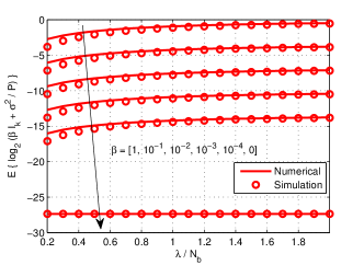
Figure 1: The accuracy of the approximation of $\mathbb{E}\{\log_{2}(\beta I_{k}+\frac{\sigma^{2}}{P})\}$.

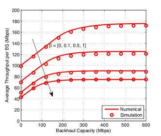
(a) Average throughput versus $C_{\rm bh}$, $\eta=0.1$.

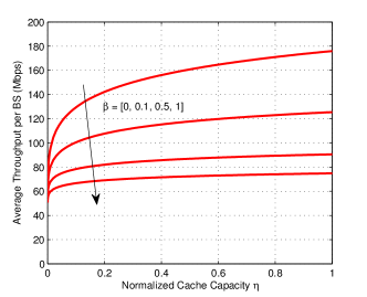
(b) Average throughput versus $\eta$, $C_{\rm bh}=100$Mbps.

Figure 2: Average throughput versus backhaul capacity and cache capacity.

To validate the approximation introduced in (C.1), we compare the simulation results of the average throughput per cell with the numerical results obtained from (16) versus $C_{\rm bh}$ in Fig. 2(a). We can see that the simulation and numerical results almost overlap, i.e., the approximation is accurate, although $N_{t}=4$ and $N_{b}=37$ that are far from infinity. To show the impact of caching on the throughput of the network, we also provide the numerical results obtained from (16) versus $\eta$ in Fig. 2(b). We can see from Fig. 2(a) and Fig. 2(b) that the throughput increases with both the backhaul capacity and cache capacity, which agrees with the result in (25) derived in the special scenario. Moreover, the throughput increases with $\eta$ more sharply when $\beta$ is small. This suggests that the throughput can be boosted more efficiently by caching at the BSs if the ICI level can be reduced.

V-B When EE Benefits from Caching?

In Table I, we use numerical results to show when the condition in (34) holds for different content catalog size $N_{f}$, backhaul hardware and cache hardware.

A typical pico BS in LTE system is considered, where the transmission and power consumption parameters have been defined in the beginning of this section. The interference level is set as $\beta=1$. In such a worst case, the condition is more prone to be invalid. While there are various kinds of memory technologies, we consider the two kinds that are most likely employed due to their higher power efficiencies and larger cache sizes. Except for the high speed SSD cache hardware with $w_{\rm ca}=6.25\times 10^{-12}$ W/bit and microwave backhaul link with $w_{\rm bh}=5\times 10^{-7}$ J/bit, we also consider DRAM as cache hardware and optical fiber as backhaul link (with capacity $1$ Gbps), whose power coefficients are respectively $w_{\rm ca}=2.5\times 10^{-9}$ W/bit [9] and $w_{\rm bh}=4\times 10^{-8}$ J/bit [9, 14]. Considering that $N_{f}$ has a wide range in literatures, e.g., $N_{f}=10^{2}\sim 10^{3}$ with a large content size $F=10^{2}\sim 10^{3}$ MB [39, 40] and $N_{f}=10^{4}\sim 10^{5}$ with a small content size $F=1\sim 10$ MB [12, 41], we also investigate the impact of $N_{f}$ and $F$ on the condition.

TABLE I: Numerical Example, $\delta=1$

Condition	(34)		$w_{\rm ca}$	$w_{\rm bh}$	$N_{f}$	$F$
	LHS	RHS
Hold	$0.006$	$34.4$	SSD	microwave	$10^{5}$	$10$ MB
Hold	$0.006$	$2.31$	SSD	optical fiber	$10^{5}$	$10$ MB
Hold	$0.37$	$2.31$	SSD	optical fiber	$10^{3}$	$10^{3}$ MB
Hold	$2.41$	$34.4$	DRAM	microwave	$10^{5}$	$10$ MB
Not hold	$2.41$	$2.31$	DRAM	optical fiber	$10^{5}$	$10$ MB
Not hold	$149.7$	$34.4$	DRAM	microwave	$10^{3}$	$10^{3}$ MB

As expected, when the values of $w_{\rm ca}$ is large and $w_{\rm bh}$ is small, the EE does not benefit from caching at the BSs. Moveover, with the same value of $N_{f}F$, the condition is more prone to be invalid when the content size $F$ is large.

V-C Impact of Key Parameters on EE

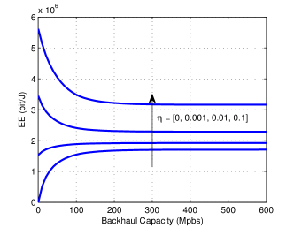
(a) EE versus backhaul capacity, $\beta=0.5$.

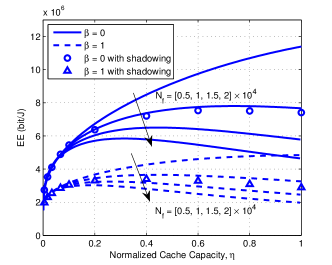
(b) EE versus the cache capacity, $C_{\rm bh}=100$ Mbps.

Figure 3: EE versus backhaul capacity and cache capacity.

In Fig. 3, we show the numerical results of EE obtained from (24) respectively versus backhaul capacity and normalized cache capacity. We can see from Fig. 3(a) that when no content or a little portion of the contents are cached at each BS (i.e., $\eta=0$ and $0.001$), EE increases with the backhaul capacity, and when the portion is large (i.e., $\eta=0.01,0.1$), EE decreases with $C_{\rm bh}$. This is because although the throughput increases with $C_{\rm bh}$, the backhaul power consumption also increases with more backhaul traffic. Moreover, the EE gain of caching over not caching is high when the backhaul capacity is very limited, and the gain approaches a constant when $C_{\rm bh}$ is large, say 200 Mbps. Fig. 3(b) shows that when the catalog size $N_{f}$ is relatively small (i.e., $N_{f}<N_{th}$), say $N_{f}=5000$, EE increases with $\eta$ until all contents are cached, and the maximal EE gain of caching over not caching is about 575% when $\beta=0$ and 250% when $\beta=1$. When $N_{f}$ is large (i.e., $N_{f}>N_{th}$), EE first increases and then decreases with $\eta$. In fact, we can compute the values of $N_{th}$ from (43) for unlimited-capacity backhaul or numerically from (38) for limited-capacity backhaul. In the considered setting, the values of $N_{th}$ range from 3000 to 20000 contents. Note that these results are obtained when each BS can schedule at most $N_{t}$ users. Nonetheless, the results are consistent with the analysis in Section IV-A and Proposition 2, which are obtained in the special case where each BS only serves at most one user. By comparing Fig. 3(b) with Fig. 2(b), we can see that the EE gain from caching is much higher than the throughput gain from caching if ICI can be perfectly controlled (i.e., $\beta=0$). This is because when backhaul capacity is limited, the throughput gain of caching only comes from reducing ICI, but the EE gain also comes from reducing the proportion of power consumed for backhauling. To show the impact of shadowing, we also provide the simulation result of EE in Fig. 3(b), where the shadowing is subject to log-normal distribution with 8 dB deviation. We can see that the network EE is slightly lower when shadowing is considered but the main trend of EE-cache relationship does not change.

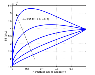
(a) EE versus $\eta$ under different skew parameter $\delta$.

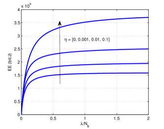
(b) EE versus $\frac{\lambda}{N_{b}}$ under different cache capacity $\eta$.

Figure 4: EE versus cache capacity and user density, $\beta=0.5$, $C_{\rm bh}=100$ Mbps.

In Fig. 4(a), we show the numerical results of EE obtained from (24) versus the normalized cache capacity with different skew parameter $\delta$. We can see that the optimal cache capacity decreases with $\delta$. With the same cache capacity, EE increases with $\delta$. This is because the cache hit ratio increases with $\delta$ as shown in (9). When $\delta=1$, the EE gain of caching with optimized $\eta$ over not caching is about 350%. In Fig. 4(b), we show the numerical results of EE obtained from (24) versus the ratio of user density to BS density. We can see that EE first increases with $\frac{\lambda}{N_{b}}$ quickly and then saturates gradually because the throughput is finally limited by ICI. Moreover, the EE increases more sharply when cache is enabled. This is because the throughput is increased and the backhaul power consumption is reduced by caching. When $\frac{\lambda}{N_{b}}$ is around one, which is typical for SCNs, the EE gain is about 230%.

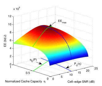
(a) $C_{\rm bh}\to\infty$

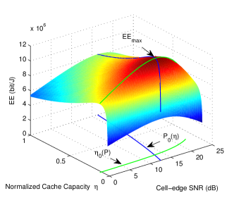
(b) $C_{\rm bh}\to 0$

Figure 5: EE versus cell-edge SNR and normalized cache capacity, $\beta=0$, $\delta=1$.

In Fig. 5, we show the numerical results of EE obtained from (33) versus the cell-edge SNR (which is controlled by changing the transmit power and hence reflects the impact of transmit power) and normalized cache capacity under unlimited-capacity backhaul and very stringent-capacity backhaul. As we analyzed in section IV-B, with a given cache capacity, the EE first increases with $P$ and then decreases with $P$. We also plot the optimal transmit power $P_{0}$ as a function of $\eta$ denoted as $P_{0}(\eta)$, as well as the optimal normalized cache capacity $\eta_{0}$ as a function of $P$ denoted as $\eta_{0}(P)$. We can see that $P_{0}(\eta)$ increases with $\eta$ slowly as we analyzed in Section IV-B, and $\eta_{0}(P)$ increases with $P$ slowly with very stringent-capacity backhaul. This implies that in a cache-enabled network with stringent-capacity backhaul, the value of transmit power has minor impact on the EE-optimal cache capacity and the value of cache capacity has little impact on the optimal transmit power. Besides, it is easy to find that the joint optimal values of $\eta$ and $P$ maximizing the network EE is the crossing point of $\eta_{0}(P)$ and $P_{0}(\eta)$. This means that $(P_{0},\eta_{0})$ satisfying both $\frac{dEE}{dP}=0$ in (47) and $\frac{dEE}{d\eta}=0$ in (42) are the joint optimal transmit power and cache capacity with the considered system setting, although the EE is not joint concave in $P$ and $\eta$ as we analyzed in Section IV-B.

V-D Where to Cache Can Provide Higher EE?

To illustrate where to deploy the caches can provide higher EE, we compare the throughput and EE achieved by caching at the macro and pico BSs. For a fair comparison, we deploy three tiers of macro BSs similar to the pico network. The radius of each macro cell is $250$ m, i.e., the coverage area of each macro cell is the same as that of $N_{b}=37$ pico cells. To ensure that the pico network and the macro network have the same total number of antennas and the same sum backhaul capacity within the same coverage area, each macro BSs is equipped with $4\times 37$ antennas and the backhaul capacity for each pico BS and macro BS is $100$ Mbps and $100\times 37$ Mbps. The power consumption parameters of the macro BS are $\rho=3.22$, $P=46$ dBm, $P_{{\rm cc}_{i}}=2.01\times 10^{3}$ W ($13.6$ W per antenna), $P_{{\rm cc}_{a}}=3.81\times 10^{3}$ W ($25.8$ W per antenna) [27]. If each BS caches $N_{c}$ contents, the total cache capacities of the macro and pico networks will be $N_{c}F$ and $N_{b}N_{c}F$, respectively. In this simulation, we set the two networks with the same total cache capacity, hence each pico BS caches less contents.

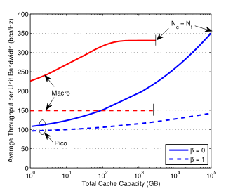
(a) Throughput

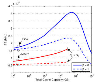
(b) EE

Figure 6: Throughput and EE comparison between macro and pico networks, $N_{f}=10^{5}$. The throughput is evaluated within a region of 250 m radius including one macro cell and $37$ pico cells. The curves stop when $N_{c}=N_{f}$, i.e, all contents are cached at each BS. The curves of pico network stop earlier because each pico BS caches less contents than each macro BS because the two networks are set with identical total cache capacity.

We can see from Fig. 6(a) that when the total cache capacity of the network is low, the throughput of the macro network is higher than the pico network due to higher backhaul capacity for each BS. When $\beta=1$, the throughput of the macro network does not change with cache capacity, but the throughput of the pico network increases with cache capacity. This is because the backhaul capacity of each macro BS is large such that interference is the limiting factor of throughput, while the backhaul capacity of each pico BS network is low so that increasing cache capacity can relieve the backhaul congestion and hence increase the throughput. When there is no interference and $\beta=0$, backhaul capacity becomes the bottleneck of both networks and thus their throughputs increase with cache capacity. We can see from Fig. 6(b) that the EE of the pico network is higher than the macro network since the pico BSs have more opportunities to idle and have low transmit and circuit powers although the cache capacity of each pico BS is smaller than each macro BS. The EE of the pico networks benefits more from caching, despite that more replicas of the same content are cached. This is because the backhaul capacity limits the throughput of each pico BS meanwhile the backhaul power consumption takes a large portion of the energy consumed in the pico network.

V-E Impact of User Association

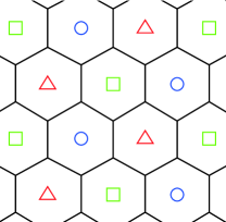
(a) An illustration of distributed caching.

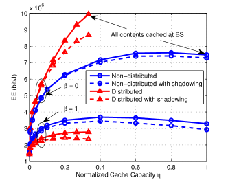
(b) EE comparison, $C_{\rm bh}=100$ Mbps.

Figure 7: Impact of user association with distributed caching and shadowing.

In the system model, we have assumed that each user is associated with the closest BS, and hence caching most popular contents in each BS is optimal. Now we relax this assumption and consider a user association based on both location and content. As shown in (33), EE increases with the cache hit ratio $p_{h}$. To increase $p_{h}$, we consider a distributed caching strategy where every three adjecent BSs cache different contents and each user associates with the nearest BS that caches the user’s requested contents. As illustrated in Fig. 7(a), the BS marked with “$\Delta$” caches the $1$st, $4$th, $7$th, $\cdots$, $(3N_{c}-2)$th popular contents, the BS marked with “$\square$” caches the $2$nd, $5$th, $8$th, $\cdots$, $(3N_{c}-1)$th popular contents, and the BS marked with “$\bigcirc$” caches the $3$rd, $6$th, $9$th, $\cdots$, $3N_{c}$th popular contents. This way of caching can reduce content redundancy by storing different contents in different BSs. Then, when each BS caches $N_{c}$ contents with the distributed caching, each user can access to $3N_{c}$ cached contents, i.e, the equivalent cache capacity seen from each user can be regarded as three times over that with non-distributed caching.

In Fig. 7(b), we show the simulation results of EE with distributed caching and non-distributed caching. We can see that when $\beta=0$, i.e., no interference, distributed caching can achieve higher EE due to higher cache hit ratio. When $\beta=1$, i.e., in the worst case of interference, distributed caching achieves lower EE than non-distributed caching. This is because each user may not always associate with the nearest BS with distributed caching and hence the nearest BS may generate strong interference to the user, which results in the EE reduction. When shadowing is considered and each user is associated to the BS with highest average channel gain, the network EE is slightly lower but the main trend of EE-cache relationship doed not change for both non-distributed and distributed caching.

VI Conclusion

In this paper, we investigated whether and how caching at BSs can improve EE of wireless access networks. By analyzing the EE for the cache-enabled network, we found the condition of whether EE can benefit from caching, the EE-memory relation, and the maximal EE gain from caching. Analytical results showed that EE can be improved by caching at the BSs when power efficient cache hardware is used. A key observation is that the EE gain of caching comes from boosting the throughput, reducing the backhaul consumption and exploiting the content popularity when the backhaul is limited. The EE gain is large when the interference level is low, the backhaul capacity is stringent, and the content popularity distribution is skewed. Another key observation is that EE-memory relation is not a simple tradeoff. When the content catalog size is not very large, there is a tradeoff between EE and cache capacity. Otherwise, optimizing cache capacity of each BS can maximize the EE of the network. The EE-optimal cache capacity depends on the system setting, and decreases when the network becomes denser. Numerical and simulation results validated the analysis and showed that caching at pico BS can provide higher EE gain than caching at macro BS. Finally, we provided simulation results to illustrate that distributed caching will achieve much higher EE gain than simply caching popular contents everywhere if inter-cell interference can be successfully eliminated, but will be inferior to the simple caching policy if the interference can not be coordinated.

Appendix A Proof of Lemma 1

Considering that the SINRs for the users shown in (3) are identically distributed, $\bar{R}_{\rm ca}(K_{b},K_{c})$ can be derived as

$$\bar{R}_{\rm ca}(K_{b},K_{c})=K_{c}B\mathbb{E}\left\{\log_{2}\left(1+\frac{r_{kb}^{-\alpha}|\mathbf{h}_{kb}^{H}\mathbf{w}_{kb}|^{2}}{K_{b}(\beta I_{k}+\frac{\sigma^{2}}{P})}\right)\right\}$$

$$\overset{(a)}{\approx}K_{c}B\Bigg{(}\mathbb{E}\left\{\log_{2}|\mathbf{h}_{kb}^{H}\mathbf{w}_{kb}|^{2}\right\}-\log_{2}K_{b}+\mathbb{E}\{\log_{2}r_{kb}^{-\alpha}\}$$

$$\quad~{}-\mathbb{E}\left\{\log_{2}\left(\beta I_{k}+\frac{\sigma^{2}}{P}\right)\right\}\Bigg{)}$$

$$\overset{(b)}{=}K_{c}B\Bigg{(}\frac{1}{\ln 2}\psi(N_{t}-K_{b}+1)-\log_{2}K_{b}$$

$$\quad~{}+\int_{0}^{D}\log_{2}\left(r_{kb}^{-\alpha}\right)\frac{2r_{kb}}{D^{2}}dr_{kb}-\mathbb{E}\left\{\log_{2}\left(\beta I_{k}+\frac{\sigma^{2}}{P}\right)\right\}\Bigg{)}$$

$$\overset{(c)}{\approx}K_{c}B\Bigg{(}\log_{2}\frac{N_{t}-K_{b}+1}{K_{b}}+\frac{\alpha}{2\ln 2}+\log_{2}D^{-\alpha}$$

$$\quad~{}-\mathbb{E}\left\{\log_{2}\left(\beta I_{k}+\frac{\sigma^{2}}{P}\right)\right\}\Bigg{)}$$ (A.1)

where the approximation in step $(a)$ is from omitting the term “$1$” inside the log function, which is accurate in high SINR region, step $(b)$ comes from the facts that $|\mathbf{h}_{kb}^{H}\mathbf{w}_{kb}|^{2}$ follows Gamma distribution $\mathbb{G}(N_{t}-K_{b}+1,1)$ [42] and $\frac{2r_{kb}}{D^{2}}$ is the probability density function (PDF) of $r_{kb}$ when the user is uniformly distributed in the circle cell, and step $(c)$ is obtained by applying the asymptotic approximation of the Digamma function $\psi(n)$, i.e., $\psi(n)=\ln(n)+\mathcal{O}(\frac{1}{n})\approx\ln n$ [43] and the approximation is accurate when $N_{t}-K_{b}+1>1$.

When the network is interference-limited, i.e., the interference power $\beta PI_{k}\gg\sigma^{2}$,

$$\mathbb{E}\left\{\log_{2}\left(\beta I_{k}+\frac{\sigma^{2}}{P}\right)\right\}\approx\mathbb{E}\{\log_{2}(\beta I_{k})\}$$ (A.2)

Considering the expression of $I_{k}$ defined in (3) and $\mathbb{E}\{\zeta_{j}\}=1\cdot p_{a}+0\cdot(1-p_{a})=p_{a}$, we have

$$\mathbb{E}\{\log_{2}(\beta I_{k})\}=\mathbb{E}\{\log_{2}(I_{k}D^{\alpha})\}+\log_{2}(\beta D^{-\alpha})$$ (A.3)

where $\mathbb{E}\{\log_{2}(I_{k}D^{\alpha})\}$ can be derived as

$$\mathbb{E}\{\log_{2}(I_{k}D^{\alpha})\}$$

$$=\mathbb{E}_{r_{kj},\mathbf{h}_{kj},\zeta_{j}}\left\{\log_{2}\left(\sum_{j=1,j\neq b}^{N_{b}}\zeta_{j}\left(\frac{D}{r_{kj}}\right)^{\alpha}\|\mathbf{h}_{kj}\mathbf{W}_{j}\|^{2}\right)\right\}$$

$$\overset{(a)}{\leq}\mathbb{E}_{r_{kj},\mathbf{h}_{kj}}\left\{\log_{2}\left(\sum_{j=1,j\neq b}^{N_{b}}\mathbb{E}\{\zeta_{j}\}\left(\frac{D}{r_{kj}}\right)^{\alpha}\|\mathbf{h}_{kj}\mathbf{W}_{j}\|^{2}\right)\right\}$$

$$=\mathbb{E}_{r_{kj},\mathbf{h}_{kj}}\left\{\log_{2}\left(\sum_{j=1,j\neq b}^{N_{b}}\!\left(\frac{D}{r_{kj}}\right)^{\alpha}\!\|\mathbf{h}_{kj}\mathbf{W}_{j}\|^{2}\right)\right\}\!+\log_{2}p_{a}$$

$$\triangleq\Phi+\log_{2}p_{a}=\log_{2}p_{a}2^{\Phi}$$ (A.4)

where the upper bound in step $(a)$ is from using the Jensen’s inequality and the bound is tight when $\frac{\lambda}{N_{b}}$ is high (then $p_{a}\to 1$ and hence $\zeta_{j}\to\mathbb{E}\{\zeta_{j}\}$), and $\Phi$ is a constant only depending on the path-loss exponent $\alpha$ when $N_{b}\to\infty$ (to be proved in Appendix B). By substituting (A.4) into (A.3) and then into (A.2), we obtain

$$\mathbb{E}\left\{\log_{2}\left(\beta I_{k}+\frac{\sigma^{2}}{P}\right)\right\} \leq\log_{2}(p_{a}\beta 2^{\Phi}D^{-\alpha})$$

$$\approx\log_{2}\left(p_{a}\beta 2^{\Phi}D^{-\alpha}+\frac{\sigma^{2}}{P}\right)$$ (A.5)

where the approximation comes from the fact that when $\beta PI_{k}\gg\sigma^{2}$, we have $\log_{2}(p_{a}\beta 2^{\Phi}D^{-\alpha})\geq\mathbb{E}\{\log_{2}(\beta I_{k})\}\gg\log_{2}(\frac{\sigma^{2}}{P})$ which means $p_{a}\beta 2^{\Phi}D^{-\alpha}\gg\frac{\sigma^{2}}{P}$.

When the network is noise-limited, i.e., $\beta PI_{k}\ll\sigma^{2}$, we also have $\mathbb{E}\{\log_{2}(\beta I_{k}+\frac{\sigma^{2}}{P})\}\approx\log_{2}\frac{\sigma^{2}}{P}\approx\log_{2}(p_{a}\beta 2^{\Phi}D^{-\alpha}+\frac{\sigma^{2}}{P})$, which is the same as the result in (A.5).

By substituting (A.5) into (A.1), $\bar{R}_{\rm ca}(K_{b},K_{c})$ can be approximated as

$$\bar{R}_{\rm ca}(K_{b},K_{c}) \approx K_{c}B\left(\frac{\alpha}{2\ln 2}+\log_{2}\frac{(N_{t}-K_{b}+1)P}{K_{b}(p_{a}\beta P2^{\Phi}+D^{\alpha}\sigma^{2})}\right)$$

$$\triangleq K_{c}\left(\frac{\alpha B}{2\ln 2}+\bar{R}_{\rm e}(K_{b})\right)$$ (A.6)

where $\bar{R}_{\rm e}(K_{b})\triangleq B\log_{2}\frac{(N_{t}-K_{b}+1)P}{K_{b}(p_{a}\beta P2^{\Phi}+D^{\alpha}\sigma^{2})}$ can also be derived from $\mathbb{E}\left\{B\log_{2}\frac{PD^{-\alpha}|\mathbf{h}_{kb}^{H}\mathbf{w}_{kb}|^{2}}{K_{b}(\beta PI_{k}+\sigma^{2})}\right\}$. Hence, $\bar{R}_{\rm e}(K_{b})$ can be regarded as the average achievable rate of a cell-edge user when the backhaul capacity is unlimited and BS_b serves $K_{b}$ users.

Appendix B Proof of the constant $\Phi$ when $N_{b}\to\infty$

In the following, we first prove $\Phi$ only depends on $\alpha$ and $N_{b}$, and then prove $\Phi$ converges when $N_{b}\to\infty$. Without loss of generality, we assume the coordinate of BS_b as $(0,0)$. Denoting $(x_{k},y_{k})$ and $(u_{j},v_{j})$ as the coordinate of MS_k and BS_j, respectively, then $r_{kb}=\sqrt{x_{k}^{2}+y_{k}^{2}}$ and $r_{kj}=\sqrt{(x_{k}-u_{j})^{2}+(y_{k}-v_{j})^{2}}$. Denoting $I_{kj}\triangleq\|\mathbf{h}_{kj}\mathbf{W}_{j}\|^{2}$ and taking the expectation over user location in (A.4), we obtain

$$\Phi=\frac{1}{\pi D^{2}}\iint_{x_{k}^{2}+y_{k}^{2}\leq D^{2}}\mathbb{E}_{I_{kj}}\Bigg{\{}\log_{2}\Bigg{(}\sum_{j=1,j\neq b}^{N_{b}}\\ \left(\frac{D}{\sqrt{(x_{k}-u_{j})^{2}+(y_{k}-v_{j})^{2}}}\right)^{\alpha}\!I_{kj}\Bigg{)}\Bigg{\}}dx_{k}dy_{k}$$ (B.1)

We normalize the coordinates of MS_k and BS_j with the cell radius $D$ as $(\bar{x}_{k},\bar{y}_{k})=\big{(}\frac{x_{k}}{D},\frac{y_{k}}{D}\big{)}$ and $(\bar{u}_{j},\bar{v}_{j})=\big{(}\frac{u_{j}}{D},\frac{v_{j}}{D}\big{)}$, respectively. After changing the integration variables as $\bar{x}_{k}$ and $\bar{y}_{k}$, (B.1) can be rewritten as

$$\Phi=\frac{1}{\pi}\iint_{\bar{x}_{k}^{2}+\bar{y}_{k}^{2}\leq 1}\mathbb{E}_{I_{kj}}\Bigg{\{}\log_{2}\Bigg{(}\sum_{j=1,j\neq b}^{N_{b}}\\ \left((\bar{x}_{k}-\bar{u}_{j})^{2}+(\bar{y}_{k}-\bar{v}_{j})^{2}\right)^{-\frac{\alpha}{2}}I_{kj}\Bigg{)}\Bigg{\}}d\bar{x}_{k}d\bar{y}_{k}$$ (B.2)

Since the normalized coordinates $(\bar{x}_{k},\bar{y}_{k})$ and $(\bar{u}_{j},\bar{v}_{j})$ do not depend on $D$, and $I_{kj}$ is averaged over small-scale fading channel in (B.2), $\Phi$ only depend on $\alpha$ and $N_{b}$.

By using the Jensen’s inequality in (B.2) to move the expectation into the $\log$ function and considering $\mathbb{E}\{I_{kj}\}=1$, we obtain

$$\Phi\leq\frac{1}{\pi}\iint_{\bar{x}_{k}^{2}+\bar{y}_{k}^{2}\leq 1}\log_{2}\Bigg{(}\sum_{j=1,j\neq b}^{N_{b}}\\ \left((\bar{x}_{k}-\bar{u}_{j})^{2}+(\bar{y}_{k}-\bar{v}_{j})^{2}\right)^{-\frac{\alpha}{2}}\Bigg{)}d\bar{x}_{k}d\bar{y}_{k}$$ (B.3)

Considering $\alpha>2$ in practice and after some manipulations, we can show that $\sum_{j=1,j\neq b}^{N_{b}}\big{(}(\bar{x}_{k}-\bar{u}_{j})^{2}+(\bar{y}_{k}-\bar{v}_{j})^{2}\big{)}^{-\frac{\alpha}{2}}$ converges when $N_{b}\to\infty$. Therefore, $\Phi$ has an upper bound. Further considering $\Phi$ increases with $N_{b}$, $\Phi$ converges when $N_{b}\to\infty$.

Appendix C Proof of Lemma 2

Consider that when $N_{t}\to\infty$, $\mathbb{E}_{\mathbf{h}_{kb}}\big{\{}\frac{|\mathbf{h}_{kb}\mathbf{w}_{kb}|^{2}}{N_{t}}\big{\}}\to 1$ and the variance of $\frac{|\mathbf{h}_{kb}\mathbf{w}_{kb}|^{2}}{N_{t}}$ approaches to zero resulting from channel hardening [44]. Besides, when the interference power from each BS is independent and identically distributed (i.i.d.), the interference power per BS $\frac{\beta PI_{k}}{N_{b}}=\frac{\beta P}{N_{b}}\sum_{j=1,j\neq b}^{N_{b}}\zeta_{j}r_{kj}^{-\alpha}\|\mathbf{h}_{kj}\mathbf{W}_{j}\|^{2}$ approaches to its expectation $\frac{\beta P}{N_{b}}\mathbb{E}\{I_{k}\}$ when $N_{b}\to\infty$ according to the law of large numbers. This suggests that the distance between each user and its local BS $r_{kb}$ dominates the comparison between $\sum_{k=K_{c}+1}^{K_{b}}B\log_{2}(1+\gamma_{k})$ and $C_{\rm bh}$ when $N_{b}$ is large, and therefore the second term in (10) can be approximated as

$$\bar{R}_{\rm bh}(K_{b},K_{c},C_{\rm bh})=\mathbb{E}\left\{\min\left(B\!\!\sum_{k=K_{c}+1}^{K_{b}}\!\!\log_{2}(1+\gamma_{k}),C_{\rm bh}\right)\right\}$$

$$\approx\mathbb{E}_{r_{kb}}\left\{\min\left(B\!\!\sum_{k=K_{c}+1}^{K_{b}}\!\!\mathbb{E}_{\mathbf{h},r_{kj},\zeta_{j}}\big{\{}\log_{2}(1+\gamma_{k})\big{\}},C_{\rm bh}\right)\right\}$$ (C.1)

which is accurate as shown via simulations in Section V-A.

By omitting the term “$1$” inside the log function, approximating $\psi(n)$ by $\ln(n)$ similar to the derivation for (A.1), and further considering (A.5) and the definition of $\bar{R}_{\rm e}(K_{b})$, we have

$$\mathbb{E}_{\mathbf{h},r_{kj},\zeta_{j}}\big{\{}\log_{2}(1+\gamma_{k})\big{\}}\approx\log_{2}\frac{(N_{t}-K_{b}+1)P}{K_{b}(p_{a}\beta P2^{\Phi}D^{-\alpha}+\sigma^{2})}\\ +\log_{2}r_{kb}^{-\alpha}=\frac{\bar{R}_{\rm e}({K_{b}})}{B}+\alpha\log_{2}\frac{D}{r_{kb}}$$ (C.2)

By substituting (C.2) into (C.1), we obtain

$$\bar{R}_{\rm bh}(K_{b},K_{c},C_{\rm bh})\approx\mathbb{E}_{r_{kb}}\Bigg{\{}\min\Bigg{(}(K_{b}-K_{c})\bar{R}_{\rm e}(K_{b})\\ +\frac{\alpha B}{2\ln 2}\sum_{k=K_{c}+1}^{K_{b}}\!\!\!2\ln\frac{D}{r_{kb}},C_{\rm bh}\Bigg{)}\Bigg{\}}\triangleq\mathbb{E}_{r_{kb}}\{\tilde{R}_{\rm bh}\}$$ (C.3)

where we define $\tilde{R}_{\rm bh}$ to denote the term inside $\mathbb{E}_{r_{kb}}\{\cdot\}$ in (C.3) for notation simplicity.

With the PDF of $r_{kb}$, i.e., $\frac{2r_{kb}}{D^{2}}$, we can prove that $\{2\ln\frac{D}{r_{kb}},k=1,\cdots,K_{b},b=1,\cdots,N_{b}\}$ are independent exponential distributed RVs with unit mean. Hence, the term $y\triangleq\sum_{k=K_{c}+1}^{K_{b}}2\ln\frac{D}{r_{kb}}$ in (C.3) is a Gamma distributed RV following $\mathbb{G}(K_{b}-K_{c},1)$, i.e., it is positive, and the PDF of this term is $f(y)=\frac{y^{K_{b}-K_{c}-1}e^{-y}}{(K_{b}-K_{c}-1)!}$, $y>0$. This gives rise to the following results.

When $C_{\rm bh}\leq(K_{b}-K_{c})\bar{R}_{\rm e}(K_{b})$, i.e., the backhaul capacity is less than the average achievable sum-rate of all the cache-miss users under unlimited-capacity backhaul when they are located at the cell edge, the right hand side (RHS) of (C.3) becomes

$$\mathbb{E}_{r_{kb}}\{\tilde{R}_{\rm bh}\}=C_{\rm bh}$$ (C.4)

When $C_{\rm bh}>(K_{b}-K_{c})\bar{R}_{\rm e}(K_{b})$, considering

$$\tilde{R}_{\rm bh}=\left\{\begin{array}[]{l l}(K_{b}-K_{c})\bar{R}_{\rm e}(K_{b})+\frac{\alpha B}{2\ln 2}y,&\text{if}~{}y<z\\ C_{\rm bh},&\text{if}~{}y\geq z\end{array}\right.$$ (C.5)

where $z\triangleq\frac{2\ln 2}{\alpha B}\big{(}C_{\rm bh}-(K_{b}-K_{c})\bar{R}_{\rm e}(K_{b})\big{)}$, the RHS of (C.3) can be derived as

$$\mathbb{E}_{r_{kb}}\{\tilde{R}_{\rm bh}\}$$

$$=\int_{0}^{\infty}\min\left((K_{b}-K_{c})\bar{R}_{\rm e}(K_{b})+\frac{\alpha B}{2\ln 2}y,C_{\rm bh}\right)f(y)dy$$

$$=\int_{0}^{z}\left((K_{b}-K_{c})\bar{R}_{\rm e}(K_{b})+\frac{\alpha B}{2\ln 2}y\right)f(y)dy$$

$$\quad+\int_{z}^{\infty}C_{\rm bh}f(y)dy$$

$$=(K_{b}-K_{c})\bigg{(}\frac{\alpha B}{2\ln 2}\gamma(K_{b}-K_{c}+1,z)$$

$$\quad+\bar{R}_{\rm e}(K_{b})\gamma(K_{b}-K_{c},z)\bigg{)}+C_{\rm bh}\Gamma(K_{b}\!-K_{c},z)$$ (C.6)

Combine (C.4) and (C.6), Lemma 2 is proved.

Appendix D Proof of Proposition 1

With $N_{c}=0$ and $p_{h}=0$, from (33) the EE without caching can be obtained as $EE_{\rm no}=\frac{p_{a}\bar{R}_{\rm bh}}{p_{a}P_{a}+(1-p_{a})P_{i}+p_{a}w_{\rm bh}\bar{R}_{\rm bh}}$. If $EE_{\rm no}$ exceeds the EE with caching in (33), then with (9) we have

$$w_{\rm ca}N_{c}F\sum_{j=1}^{N_{f}}j^{-1}>\\ \big{(}(p_{a}P_{a}+(1-p_{a})P_{i})\bar{R}_{\rm ca}+p_{a}w_{\rm bh}\bar{R}_{\rm ca}\bar{R}_{\rm bh}\big{)}\sum_{f=1}^{N_{c}}f^{-1}$$ (D.1)

If (D.1) holds for $N_{c}=1$ , then

$$w_{\rm ca}F\sum_{j=1}^{N_{f}}j^{-1}>\big{(}(p_{a}P_{a}+(1-p_{a})P_{i})\bar{R}_{\rm ca}+p_{a}w_{\rm bh}\bar{R}_{\rm ca}\bar{R}_{\rm bh}\big{)}$$ (D.2)

Multiplying both side of (D.2) by $N_{c}$, we obtain

$$w_{\rm ca}N_{c}F\sum_{j=1}^{N_{f}}j^{-1}>\\ \big{(}(p_{a}P_{a}+(N_{b}-p_{a})P_{i})\bar{R}_{\rm ca}+p_{a}w_{\rm bh}\bar{R}_{\rm ca}\bar{R}_{\rm bh}\big{)}N_{c}$$ (D.3)

Furthering considering that $N_{c}>\sum_{f=1}^{N_{c}}f^{-1}$ for $N_{c}>1$, (D.3) turns into

$$w_{\rm ca}N_{c}F\sum_{j=1}^{N_{f}}j^{-1}>\\ \big{(}(p_{a}P_{a}+(1-p_{a})P_{i})\bar{R}_{\rm ca}+p_{a}w_{\rm bh}\bar{R}_{\rm ca}\bar{R}_{\rm bh}\big{)}\sum_{f=1}^{N_{c}}f^{-1}$$ (D.4)

which is the same as (D.1). This suggests that if caching one content can not improve EE, then for any $N_{c}>1$ caching can not improve EE. Therefore, (D.2) is the condition of whether caching can increase EE. (D.2) can be rewritten as (34), and Proposition 1 is proved.

Appendix E Proof of Proposition 2

From $\frac{dEE}{d\eta}\big{|}_{\eta=\eta_{0}}=0$, we can obtain $\frac{\Omega}{\eta_{0}N_{f}}+\ln\frac{1}{\eta_{0}N_{f}}=\frac{\bar{R}_{\rm bh}}{\bar{R}_{\rm ca}-\bar{R}_{\rm bh}}\ln N_{f}-1$. Adding $\ln\Omega$ on both sides of the equation, we obtain

$$\frac{\Omega}{\eta_{0}N_{f}}+\ln\frac{\Omega}{\eta_{0}N_{f}}=\ln\Omega+\frac{\bar{R}_{\rm bh}}{\bar{R}_{\rm ca}-\bar{R}_{\rm bh}}\ln N_{f}-1$$ (E.1)

Taking the exponential of both sides of (E.1), we have $\frac{\Omega}{\eta_{0}N_{f}}e^{\frac{\Omega}{\eta_{0}N_{f}}}=\Omega e^{\frac{\bar{R}_{\rm bh}}{\bar{R}_{\rm ca}-\bar{R}_{\rm bh}}\ln N_{f}-1}$. Since $W(x)$ satisfies $W(x)e^{W(x)}=x$, we obtain

$$\frac{\Omega}{\eta_{0}N_{f}}=W\left(\Omega e^{\frac{\bar{R}_{\rm bh}}{\bar{R}_{\rm ca}-\bar{R}_{\rm bh}}\ln N_{f}-1}\right)$$ (E.2)

Since $\frac{\Omega}{\eta N_{f}}+\ln\frac{\Omega}{\eta N_{f}}$ decreases with $\eta$, $\frac{dEE}{d\eta}>0$ when $\eta<\eta_{0}$ and $\frac{dEE}{d\eta}<0$ when $\eta>\eta_{0}$. Rewriting (E.2) as (38) and further considering $\eta\leq 1$, Proposition 2 can be proved.

Appendix F Proof of Corollary 4

Denote $N_{b}\pi D^{2}\triangleq c$, where $c$ is a constant. Substituting $D=(\frac{c}{\pi N_{b}})^{\frac{1}{2}}$ and $p_{a}=1-e^{-\frac{\lambda}{N_{b}}}$ into (42) and then taking the derivation of $\eta_{0}$ in (42) with respect to $N_{b}$, we obtain

$$\frac{d\eta_{0}}{dN_{b}}=\frac{-w_{\rm bh}B}{2N_{b}w_{\rm ca}FN_{f}\ln N_{f}\ln 2}\Bigg{(}\frac{\frac{2\lambda}{N_{b}}e^{-\frac{\lambda}{N_{b}}}+\alpha\left(1-e^{-\frac{\lambda}{N_{b}}}\right)}{1+\beta 2^{\Phi}D^{\alpha}\left(1-e^{-\frac{\lambda}{N_{b}}}\right)}\\ +\frac{\lambda}{N_{b}}e^{-\frac{\lambda}{N_{b}}}\left(\alpha-2+\log_{2}\frac{N_{t}}{p_{a}\beta 2^{\Phi}+\left(\frac{P}{D^{\alpha}\sigma^{2}}\right)^{-1}}\right)\Bigg{)}$$ (F.1)

Since the path-loss exponent $\alpha>2$, we have $\frac{d\eta_{0}}{dN_{b}}<0$, i.e., $\eta_{0}$ decreases with $N_{b}$.

When $\frac{\lambda}{N_{b}}\to 0$, we have $p_{a}=1-e^{-\frac{\lambda}{N_{b}}}\to\frac{\lambda}{N_{b}}$. Then from (42), $\eta_{0}N_{b}$ can be expressed as

$$\eta_{0}N_{b}\to\frac{\lambda w_{\rm bh}B}{w_{\rm ca}FN_{f}\ln N_{f}}\log_{2}\frac{N_{t}}{\frac{\lambda}{N_{b}}\beta 2^{\Phi}+\big{(}\frac{P}{D^{\alpha}\sigma^{2}}\big{)}^{-1}}$$ (F.2)

from which we can see that $\eta_{0}N_{b}$ increases with $N_{b}$.

Appendix G Proof of Corollary 7

By substituting $p_{a}\beta P2^{\Phi}\ll D^{\alpha}\sigma^{2}$ into (46) and letting $\frac{dEE}{dP}\big{|}_{P=P_{0}}=0$, we obtain

$$\bar{P}_{{\rm cc}}+\bar{P}_{\rm ca}-p_{a}\rho P_{0}\left(\ln\frac{N_{t}P_{0}}{D^{\alpha}\sigma^{2}}+\frac{\alpha}{2}-1\right)=0$$ (G.1)

where $\bar{P}_{\rm cc}=p_{a}P_{{\rm cc}_{a}}+(1-p_{a})P_{{\rm cc}_{i}}$ is the average circuit power consumption of each BS, and $\bar{P}_{\rm ca}=w_{\rm ca}\eta N_{f}F$ is the average cache power consumption of each BS. From this equation we can derive (47). Since in practice the path-loss exponent $\alpha>2$, $\ln\frac{N_{t}P_{0}}{D^{\alpha}\sigma^{2}}+\frac{\alpha}{2}-1>0$ and the left hand side (LHS) of (G.1) decreases with $P_{0}$. Therefore, $\frac{dEE}{dP}>0$ when $P<P_{0}$ and $\frac{dEE}{dP}<0$ when $P>P_{0}$, which indicates that $P_{0}$ is the optimal transmit power maximizing the network EE.

Dong Liu (S’13) received the B.S. degree in electronics engineering from Beihang University (formerly Beijing University of Aeronautics and Astronautics), Beijing, China in 2013. He is currently pursuing Ph.D degree in signal and information processing with the School of Electronics and Information Engineering, Beihang University. His research interests lie in the area of caching in wireless network and cooperative transmission.

Chenyang Yang (SM’08) received the Ph.D. degree in electrical engineering from Beihang University (formerly Beijing University of Aeronautics and Astronautics), Beijing, China, in 1997. Since 1999, she has been a Full Professor with the School of Electronic and Information Engineering, Beihang University. She has published more than 200 international journal and conference papers and filed more than 60 patents in the fields of energy-efficient transmission, coordinated multi-point, interference management, cognitive radio, relay, etc. Her recent research interests include green radio, local caching, and other emerging techniques for next generation wireless networks. Prof. Yang was the Chair of the Beijing chapter of the IEEE Communications Society during 2008-2012 and the Membership Development Committee Chair of the Asia Pacific Board, IEEE Communications Society, during 2011-2013. She has served as a Technical Program Committee Member for numerous IEEE conferences and was the Publication Chair of the IEEE International Conference on Communications in China 2012 and a Special Session Chair of the IEEE China Summit and International Conference on Signal and Information Processing (ChinaSIP) in 2013. She served as an Associate Editor for the IEEE Transactions on Wireless Communications during 2009-2014 and a Guest Editor for the IEEE Journal on Selected Topics in Signal Processing published in February 2015. She is currently an Associate Editor-in-Chief of the Chinese Journal of Communications and the Chinese Journal of Signal Processing. She was nominated as an Outstanding Young Professor of Beijing in 1995 and was supported by the First Teaching and Research Award Program for Outstanding Young Teachers of Higher Education Institutions by the Ministry of Education during 1999-2004.

References

- [1] D. Liu and C. Yang, “Will caching at base station improve energy efficiency of downlink transmission?” in Proc. IEEE GlobalSIP, 2014.
- [2] C.-L. I, C. Rowell, S. Han, Z. Xu, G. Li, and Z. Pan, “Toward green and soft: a 5G perspective,” IEEE Commun. Mag., vol. 52, no. 2, pp. 66–73, Feb. 2014.
- [3] S. Yunas, M. Valkama, and J. Niemela, “Spectral and energy efficiency of ultra-dense networks under different deployment strategies,” IEEE Commun. Mag., vol. 53, no. 1, pp. 90–100, Jan. 2015.
- [4] R. Q. Hu and Y. Qian, “An energy efficient and spectrum efficient wireless heterogeneous network framework for 5G systems,” IEEE Commun. Mag., vol. 52, no. 5, pp. 94–101, May 2014.
- [5] S. Woo, E. Jeong, S. Park, J. Lee, S. Ihm, and K. Park, “Comparison of caching strategies in modern cellular backhaul networks,” in Proc. ACM MobiSys, 2013.
- [6] B. A. Ramanan, L. M. Drabeck, M. Haner, N. Nithi, T. E. Klein, and C. Sawkar, “Cacheability analysis of HTTP traffic in an operational LTE network,” in Proc. IEEE WTS, 2013.
- [7] N. Golrezaei, A. F. Molisch, A. G. Dimakis, and G. Caire, “Femtocaching and device-to-device collaboration: A new architecture for wireless video distribution,” IEEE Commun. Mag., vol. 51, no. 4, pp. 142–149, Apr. 2013.
- [8] M. Chen and A. Ksentini, “Cache in the air: exploiting content caching and delivery techniques for 5G systems,” IEEE Commun. Mag., p. 132, Feb. 2014.
- [9] N. Choi, K. Guan, D. C. Kilper, and G. Atkinson, “In-network caching effect on optimal energy consumption in content-centric networking,” in Proc. IEEE ICC, 2012.
- [10] J. Llorca, A. M. Tulino, K. Guan, J. Esteban, M. Varvello, N. Choi, and D. C. Kilper, “Dynamic in-network caching for energy efficient content delivery,” in Proc. IEEE INFOCOM, 2013.
- [11] J. Li, B. Liu, and H. Wu, “Energy-efficient in-network caching for content-centric networking,” IEEE Commun. Lett., vol. 17, no. 4, pp. 797–800, Apr. 2013.
- [12] N. Golrezaei, K. Shanmugam, A. G. Dimakis, A. F. Molisch, and G. Caire, “Femtocaching: Wireless video content delivery through distributed caching helpers,” in Proc. IEEE INFOCOM, 2012.
- [13] E. Bastug, M. Bennis, and M. Debbah, “Living on the edge: The role of proactive caching in 5G wireless networks,” IEEE Commun. Mag., vol. 52, no. 8, pp. 82–89, Aug. 2014.
- [14] Y. Xu, Y. Li, Z. Wang, T. Lin, G. Zhang, and S. Ci, “Coordinated caching model for minimizing energy consumption in radio access network,” in Proc. IEEE ICC, 2014.
- [15] K. Poularakis, G. Iosifidis, V. Sourlas, and L. Tassiulas, “Multicast-aware caching for small cell networks,” in Proc. IEEE WCNC, 2014.
- [16] P. Xi, S. Juei-Chin, Z. Jun, and B. L. Khaled, “Joint data assignment and beamforming for backhaul limited caching networks,” in Proc. IEEE PIMRC, 2014.
- [17] M. Dehghan, A. Seetharam, B. Jiang, T. He, T. Salonidis, J. Kurose, D. Towsley, and R. K. Sitaraman, “On the complexity of optimal routing and content caching in heterogeneous networks,” in Proc. IEEE INFOCOM, 2015.
- [18] J. Hachem, N. Karamchandani, and S. N. Diggavi, “Coded caching for heterogeneous wireless networks with multi-level access,” in Proc. IEEE INFOCOM, 2014.
- [19] T. Levanen, J. Pirskanen, T. Koskela, J. Talvitie, M. Valkama et al., “Radio interface evolution towards 5G and enhanced local area communications,” IEEE Access, vol. 2, pp. 1005–1029, 2014.
- [20] Y. Wang, Z. Li, G. Tyson, S. Uhlig, and G. Xie, “Optimal cache allocation for content-centric networking,” in Proc. IEEE ICNP. IEEE, 2013.
- [21] L. Breslau, P. Cao, L. Fan, G. Phillips, and S. Shenker, “Web caching and Zipf-like distributions: Evidence and implications,” in Proc. IEEE INFOCOM, 1999.
- [22] M. Cha, P. Rodriguez, J. Crowcroft, S. Moon, and X. Amatriain, “Watching television over an IP network,” in Proc. ACM SIGCOMM IMC, 2008.
- [23] E. Mugume and D. So, “Spectral and energy efficiency analysis of dense small cell networks,” in Proc. IEEE VTC Spring, 2015.
- [24] C. Li, J. Zhang, and K. Letaief, “Throughput and energy efficiency analysis of small cell networks with multi-antenna base stations,” IEEE Trans. Wireless Commun., vol. 13, no. 5, pp. 2505–2517, May 2014.
- [25] H.-S. Jo, Y. J. Sang, P. Xia, and J. G. Andrews, “Heterogeneous cellular networks with flexible cell association: A comprehensive downlink SINR analysis,” IEEE Trans. Wireless Commun., vol. 11, no. 10, pp. 3484–3495, Oct. 2012.
- [26] T. Yoo and A. Goldsmith, “On the optimality of multiantenna broadcast scheduling using zero-forcing beamforming,” IEEE J. on Select. Areas Commun., vol. 24, no. 3, pp. 528–541, Mar. 2006.
- [27] G. Auer, O. Blume, V. Giannini, I. Godor, M. Imran, Y. Jading, E. Katranaras, M. Olsson, D. Sabella, P. Skillermark et al., “D2. 3: Energy efficiency analysis of the reference systems, areas of improvements and target breakdown,” EARTH, 2010.
- [28] Z. Chong and E. Jorswieck, “Energy-efficient power control for MIMO time-varying channels,” in Proc. IEEE GreenCom, 2011.
- [29] G. Y. Li, Z. Xu, C. Xiong, C. Yang, S. Zhang, Y. Chen, and S. Xu, “Energy-efficient wireless communications: Tutorial, survey, and open issues,” IEEE Wireless Commun. Mag., vol. 18, no. 6, pp. 28–35, Dec. 2011.
- [30] G. Auer, V. Giannini, C. Desset, I. Godor, P. Skillermark, M. Olsson, M. A. Imran, D. Sabella, M. J. Gonzalez, O. Blume et al., “How much energy is needed to run a wireless network?” IEEE Wireless Commun., vol. 18, no. 5, pp. 40–49, Oct. 2011.
- [31] A. J. Fehske, P. Marsch, and G. P. Fettweis, “Bit per joule efficiency of cooperating base stations in cellular networks,” in Proc. IEEE GLOBECOM Workshops, 2010.
- [32] A. K. Gupta, H. S. Dhillon, S. Vishwanath, and J. G. Andrews, “Downlink multi-antenna heterogeneous cellular network with load balancing,” IEEE Trans. Commun., vol. 62, no. 11, pp. 4052–4067, Nov. 2014.
- [33] R. M. Corless, G. H. Gonnet, D. E. Hare, D. J. Jeffrey, and D. E. Knuth, “On the Lambert W function,” Advances in Computational mathematics, vol. 5, no. 1, pp. 329–359, 1996.
- [34] S. Tombaz, P. Monti, K. Wang, A. V astberg, M. Forzati, and J. Zander, “Impact of backhauling power consumption on the deployment of heterogeneous mobile networks,” in Proc. IEEE GLOBECOM, 2011.
- [35] TR 36.814 V1.2.0, “Further advancements for E-UTRA physical layer aspects (release 9),” 3GPP, Jun. 2009.
- [36] J. Andrews, H. Claussen, M. Dohler, S. Rangan, and M. Reed, “Femtocells: Past, present, and future,” IEEE J. Sel. Areas Commun., vol. 30, no. 3, pp. 497–508, April 2012.
- [37] J. Park, S.-L. Kim, and J. Zander, “Asymptotic behavior of ultra-dense cellular networks and its economic impact,” in Proc. IEEE GLOBECOM, 2014.
- [38] M. Hefeeda and O. Saleh, “Traffic modeling and proportional partial caching for peer-to-peer systems,” IEEE/ACM Trans. Netw., vol. 16, no. 6, pp. 1447–1460, Dec. 2008.
- [39] E. Bastug, J.-L. Guénégo, and M. Debbah, “Proactive small cell networks,” in Proc. IEEE ICT, 2013.
- [40] C. Yang, Z. Chen, Y. Yao, and B. Xia, “Performance analysis of wireless heterogeneous networks with pushing and caching,” in Proc. IEEE ICC, 2015.
- [41] F. Pantisano, M. Bennis, W. Saad, and M. Debbah, “Match to cache: Joint user association and backhaul allocation in cache-aware small cell networks,” in Proc. IEEE ICC, 2015.
- [42] J. Zhang, M. Kountouris, J. G. Andrews, and R. W. Heath, “Multi-mode transmission for the MIMO broadcast channel with imperfect channel state information,” IEEE Trans. Commun., vol. 59, no. 3, pp. 803–814, Mar. 2011.
- [43] R. W. Heath, M. Kountouris, and T. Bai, “Modeling heterogeneous network interference using poisson point processes,” IEEE Trans. on Signal Process., vol. 61, no. 16, pp. 4114–4126, Aug. 2013.
- [44] Q. Zhang, C. Yang, and A. F. Molisch, “Downlink base station cooperative transmission under limited-capacity backhaul,” IEEE Trans. Wireless Commun., vol. 12, no. 8, pp. 3746–3759, Sept. 2013.
- [45] J. G. Andrews, F. Baccelli, and R. K. Ganti, “A tractable approach to coverage and rate in cellular networks,” IEEE Trans. Commun., vol. 59, no. 11, pp. 3122–3134, Nov. 2011.