Representing Meaning with a Combination of Logical and Distributional Models

Abstract

NLP tasks differ in the semantic information they require, and at this time no single semantic representation fulfills all requirements. Logic-based representations characterize sentence structure, but do not capture the graded aspect of meaning. Distributional models give graded similarity ratings for words and phrases, but do not capture sentence structure in the same detail as logic-based approaches. So it has been argued that the two are complementary.

We adopt a hybrid approach that combines logical and distributional semantics using probabilistic logic, specifically Markov Logic Networks (MLNs). In this paper, we focus on the three components of a practical system: 1) Logical representation focuses on representing the input problems in probabilistic logic. 2) Knowledge base construction creates weighted inference rules by integrating distributional information with other sources. 3) Probabilistic inference involves solving the resulting MLN inference problems efficiently. To evaluate our approach, we use the task of textual entailment (RTE), which can utilize the strengths of both logic-based and distributional representations. In particular we focus on the SICK dataset, where we achieve state-of-the-art results. We also release a lexical entailment dataset of 10,213 rules extracted from the SICK dataset, which is a valuable resource for evaluating lexical entailment systems.

1 Introduction

Computational semantics studies mechanisms for encoding the meaning of natural language in a machine-friendly representation that supports automated reasoning and that, ideally, can be automatically acquired from large text corpora. Effective semantic representations and reasoning tools give computers the power to perform complex applications like question answering. But applications of computational semantics are very diverse and pose differing requirements on the underlying representational formalism. Some applications benefit from a detailed representation of the structure of complex sentences. Some applications require the ability to recognize near-paraphrases or degrees of similarity between sentences. Some applications require inference, either exact or approximate. Often it is necessary to handle ambiguity and vagueness in meaning. Finally, we frequently want to learn knowledge relevant to these applications automatically from corpus data.

There is no single representation for natural language meaning at this time that fulfills all of the above requirements, but there are representations that fulfill some of them. Logic-based representations [Montague (1970), Dowty, Wall, and Peters (1981), Kamp and Reyle (1993)] like first-order logic represent many linguistic phenomena like negation, quantifiers, or discourse entities. Some of these phenomena (especially negation scope and discourse entities over paragraphs) can not be easily represented in syntax-based representations like Natural Logic [MacCartney and Manning (2009)]. In addition, first-order logic has standardized inference mechanisms. Consequently, logical approaches have been widely used in semantic parsing where it supports answering complex natural language queries requiring reasoning and data aggregation [Zelle and Mooney (1996), Kwiatkowski et al. (2013), Pasupat and Liang (2015)]. But logic-based representations often rely on manually constructed dictionaries for lexical semantics, which can result in coverage problems. And first-order logic, being binary in nature, does not capture the graded aspect of meaning (although there are combinations of logic and probabilities). Distributional models [Turney and Pantel (2010)] use contextual similarity to predict the graded semantic similarity of words and phrases [Landauer and Dumais (1997), Mitchell and Lapata (2010)], and to model polysemy [Schütze (1998), Erk and Padó (2008), Thater, Fürstenau, and Pinkal (2010)]. But at this point, fully representing structure and logical form using distributional models of phrases and sentences is still an open problem. Also, current distributional representations do not support logical inference that captures the semantics of negation, logical connectives, and quantifiers. Therefore, distributional models and logical representations of natural language meaning are complementary in their strengths, as has frequently been remarked [Coecke, Sadrzadeh, and Clark (2011), Garrette, Erk, and Mooney (2011), Grefenstette and Sadrzadeh (2011), Baroni, Bernardi, and Zamparelli (2014)].

Our aim has been to construct a general-purpose natural language understanding system that provides in-depth representations of sentence meaning amenable to automated inference, but that also allows for flexible and graded inferences involving word meaning. Therefore, our approach combines logical and distributional methods. Specifically, we use first-order logic as a basic representation, providing a sentence representation that can be easily interpreted and manipulated. However, we also use distributional information for a more graded representation of words and short phrases, providing information on near-synonymy and lexical entailment. Uncertainty and gradedness at the lexical and phrasal level should inform inference at all levels, so we rely on probabilistic inference to integrate logical and distributional semantics. Thus, our system has three main components, all of which present interesting challenges. For logic-based semantics, one of the challenges is to adapt the representation to the assumptions of the probabilistic logic [Beltagy and Erk (2015)]. For distributional lexical and phrasal semantics, one challenge is to obtain appropriate weights for inference rules [Roller, Erk, and Boleda (2014)]. In probabilistic inference, the core challenge is formulating the problems to allow for efficient MLN inference  [Beltagy and Mooney (2014)].

Our approach has previously been described in garrette:iwcs11 and beltagy:starsem13. We have demonstrated the generality of the system by applying it to both textual entailment (RTE-1 in beltagy:starsem13, SICK (preliminary results) and FraCas in Beltagy:IWCS15) and semantic textual similarity (STS) similarity [Beltagy, Erk, and Mooney (2014)], and we are investigating applications to question answering. We have demonstrated the modularity of the system by testing both Markov Logic Networks [Richardson and Domingos (2006)] and Probabilistic Soft Logic [Broecheler, Mihalkova, and Getoor (2010)] as probabilistic inference engines [Beltagy et al. (2013), Beltagy, Erk, and Mooney (2014)].

The primary aim of the current paper is to describe our complete system in detail, all the nuts and bolts necessary to bring together the three distinct components of our approach, and to showcase some of the difficult problems that we face in all three areas along with our current solutions.

The secondary aim of this paper is to show that it is possible to take this general approach and apply it to a specific task, here textual entailment [Dagan et al. (2013)], adding task-specific aspects to the general framework in such a way that the model achieves state-of-the-art performance. We chose the task of textual entailment because it utilizes the strengths of both logical and distributional representations. We specifically use the SICK dataset [Marelli et al. (2014b)] because it was designed to focus on lexical knowledge rather than world knowledge, matching the focus of our system.

Our system is flexible with respect to the sources of lexical and phrasal knowledge it uses, and in this paper we utilize PPDB [Ganitkevitch, Van Durme, and Callison-Burch (2013)] and WordNet along with distributional models. But we are specifically interested in distributional models, in particular in how well they can predict lexical and phrasal entailment. Our system provides a unique framework for evaluating distributional models on RTE because the overall sentence representation is handled by the logic, so we can zoom in on the performance of distributional models at predicting lexical  [Geffet and Dagan (2005)] and phrasal entailment. The evaluation of distributional models on RTE is the third aim of our paper. We build a lexical entailment classifier that exploits both task-specific features as well as distributional information, and present an in-depth evaluation of the distributional components.

We now provide a brief sketch of our framework [Garrette, Erk, and Mooney (2011), Beltagy et al. (2013)]. Our framework is three components, the first is the logical form which is the primary meaning representation for a sentence. The second is the distributional information which is encoded in the form of weighted logical rules (first-order formulas). For example, in its simplest form, our approach can use the distributional similarity of the words grumpy and sad as the weight on a rule that says if $x$ is grumpy then there is a chance that $x$ is also sad:

$$\forall x.grumpy(x)\to sad(x)\mid f(sim(\vec{grumpy},\vec{sad}))$$

where $\vec{grumpy}$ and $\vec{sad}$ are the vector representations of the words grumpy and sad, $sim$ is a distributional similarity measure, like cosine, and $f$ is a function that maps the similarity score to an MLN weight. A more principled, and in fact superior, choice is to use an asymmetric similarity measure to compute the weight, as we discuss below.

The third component is inference. We draw inferences over the weighted rules using Markov Logic Networks (MLN) [Richardson and Domingos (2006)], a Statistical Relational Learning (SRL) technique [Getoor and Taskar (2007)] that combines logical and statistical knowledge in one uniform framework, and provides a mechanism for coherent probabilistic inference. MLNs represent uncertainty in terms of weights on the logical rules as in the example below:

$$\forall x.\>ogre(x)\Rightarrow grumpy(x)\>|\>1.5$$ (1)

$$\forall x,y.\>(friend(x,y)\wedge ogre(x))\Rightarrow ogre(y)\>|\>1.1$$

which states that there is a chance that ogres are grumpy, and friends of ogres tend to be ogres too. Markov logic uses such weighted rules to derive a probability distribution over possible worlds through an undirected graphical model. This probability distribution over possible worlds is then used to draw inferences.

We publish a dataset of the lexical and phrasal rules that our system queries when running on SICK, along with gold standard annotations. The training and testing sets are extracted from the SICK training and testing sets respectively. The total number of rules (training + testing) is 12,510, only 10,213 are unique with 3,106 entailing rules, 177 contradictions and 6,928 neutral. This is a valuable resource for testing lexical entailment systems, containing a variety of entailment relations (hypernymy, synonymy, antonymy, etc.) that are actually useful in an end-to-end RTE system.

In addition to providing further details on the approach introduced in garrette:iwcs11 and beltagy:starsem13 (including improvements that improve the scalability of MLN inference [Beltagy and Mooney (2014)] and adapt logical constructs for probabilistic inference [Beltagy and Erk (2015)]) this paper makes the following new contributions:

• We show how to represent the RTE task as an inference problem in probabilistic logic (sections 4.1,  4.2), arguing for the use of a closed-word assumption (section 4.3).

• Contradictory RTE sentence pairs are often only contradictory given some assumption about entity coreference. For example, An ogre is not snoring and An ogre is snoring are not contradictory unless we assume that the two ogres are the same. Handling such coreferences is important to detecting many cases of contradiction (section 4.4).

• We use multiple parses to reduce the impact of misparsing (section 4.5).

• In addition to distributional rules, we add rules from existing databases, in particular WordNet [Princeton University (2010)] and the paraphrase collection PPDB [Ganitkevitch, Van Durme, and Callison-Burch (2013)] (section 5.3).

• A logic-based alignment to guide generation of distributional rules (section 5.1).

• A dataset of all lexical and phrasal rules needed for the SICK dataset (10,213 rules). This is a valuable resource for testing lexical entailment systems on entailment relations that are actually useful in an end-to-end RTE system (section 5.1).

• Evaluate a state-of-the-art compositional distributional approach  [Paperno, Pham, and Baroni (2014)] on the task of phrasal entailment (section 5.2.5).

• A simple weight learning approach to map rule weights to MLN weights (section 6.3).

• The question “Do supervised distributional methods really learn lexical inference relations?” [Levy et al. (2015)] has been studied before on a variety of lexical entailment datasets. For the first time, we study it on data from an actual RTE dataset and show that distributional information is useful for lexical entailment (section 7.1).

• marelli:semeval14 report that for the SICK dataset used in SemEval 2014, the best result was achieved by systems that did not compute a sentence representation in a compositional manner. We present a model that performs deep compositional semantic analysis and achieves state-of-the-art performance (section 7.2).

2 Background

Logical Semantics

Logical representations of meaning have a long tradition in linguistic semantics [Montague (1970), Dowty, Wall, and Peters (1981), Kamp and Reyle (1993), Alshawi (1992)] and computational semantics [Blackburn and Bos (2005), van Eijck and Unger (2010)], and commonly used in semantic parsing [Zelle and Mooney (1996), Berant et al. (2013), Kwiatkowski et al. (2013)]. They handle many complex semantic phenomena such as negation and quantifiers, they identify discourse referents along with the predicates that apply to them and the relations that hold between them. However, standard first-order logic and theorem provers are binary in nature, which prevents them from capturing the graded aspects of meaning in language: Synonymy seems to come in degrees [Edmonds and Hirst (2000)], as does the difference between senses in polysemous words [Brown (2008)]. vanEijckLappin write: “The case for abandoning the categorical view of competence and adopting a probabilistic model is at least as strong in semantics as it is in syntax.”

Recent wide-coverage tools that use logic-based sentence representations include CopestakeFlickinger, bos:step08, and lewis:tacl13. We use Boxer [Bos (2008)], a wide-coverage semantic analysis tool that produces logical forms using Discourse Representation Structures [Kamp and Reyle (1993)]. It builds on the C&C CCG (Combinatory Categorial Grammar) parser [Clark and Curran (2004)] and maps sentences into a lexically-based logical form, in which the predicates are mostly words in the sentence. For example, the sentence An ogre loves a princess is mapped to:

$$\exists x,y,z.\>ogre(x)\wedge agent(y,x)\wedge love(y)\wedge patient(y,z)\wedge princess(z)$$ (2)

As can be seen, Boxer uses a neo-Davidsonian framework [Parsons (1990)]: $y$ is an event variable, and the semantic roles $agent$ and $patient$ are turned into predicates linking $y$ to the agent $x$ and patient $z$.

As we discuss below, we combine Boxer’s logical form with weighted rules and perform probabilistic inference. lewis:tacl13 also integrate logical and distributional approaches, but use distributional information to create predicates for a standard binary logic and do not use probabilistic inference. Much earlier, hobbs:acl88 combined logical form with weights in an abductive framework. There, the aim was to model the interpretation of a passage as its best possible explanation.

Distributional Semantics

Distributional models [Turney and Pantel (2010)] use statistics on contextual data from large corpora to predict semantic similarity of words and phrases [Landauer and Dumais (1997), Mitchell and Lapata (2010)]. They are motivated by the observation that semantically similar words occur in similar contexts, so words can be represented as vectors in high dimensional spaces generated from the contexts in which they occur [Landauer and Dumais (1997), Lund and Burgess (1996)]. Therefore, distributional models are relatively easier to build than logical representations, automatically acquire knowledge from “big data”, and capture the graded nature of linguistic meaning, but they do not adequately capture logical structure [Grefenstette (2013)].

Distributional models have also been extended to compute vector representations for larger phrases, e.g. by adding the vectors for the individual words [Landauer and Dumais (1997)] or by a component-wise product of word vectors [Mitchell and Lapata (2008), Mitchell and Lapata (2010)], or through more complex methods that compute phrase vectors from word vectors and tensors [Baroni and Zamparelli (2010), Grefenstette and Sadrzadeh (2011)].

Integrating logic-based and distributional semantics

It does not seem particularly useful at this point to speculate about phenomena that either a distributional approach or a logic-based approach would not be able to handle in principle, as both frameworks are continually evolving. However, logical and distributional approaches clearly differ in the strengths that they currently possess [Coecke, Sadrzadeh, and Clark (2011), Garrette, Erk, and Mooney (2011), Baroni, Bernardi, and Zamparelli (2014)]. Logical form excels at in-depth representations of sentence structure and provides an explicit representation of discourse referents. Distributional approaches are particularly good at representing the meaning of words and short phrases in a way that allows for modeling degrees of similarity and entailment and for modeling word meaning in context. This suggests that it may be useful to combine the two frameworks.

Another argument for combining both representations is that it makes sense from a theoretical point of view to address meaning, a complex and multifaceted phenomenon, through a combination of representations. Meaning is about truth, and logical approaches with a model-theoretic semantics nicely address this facet of meaning. Meaning is also about a community of speakers and how they use language, and distributional models aggregate observed uses from many speakers.

There are few hybrid systems that integrate logical and distributional information, and we discuss some of them below.

beltagy:starsem13 transform distributional similarity to weighted distributional inference rules that are combined with logic-based sentence representations, and use probabilistic inference over both. This is the approach that we build on in this paper. lewis:tacl13, on the other hand, use clustering on distributional data to infer word senses, and perform standard first-order inference on the resulting logical forms. The main difference between the two approaches lies in the role of gradience. Lewis and Steedman view weights and probabilities as a problem to be avoided. We believe that the uncertainty inherent in both language processing and world knowledge should be front and center in all inferential processes. Tian:2014vh represent sentences using Dependency-based Compositional Semantics [Liang, Jordan, and Klein (2011)]. They construct phrasal entailment rules based on a logic-based alignment, and use distributional similarity of aligned words to filter rules that do not surpass a given threshold.

Also related are distributional models where the dimensions of the vectors encode model-theoretic structures rather than observed co-occurrences [Clark (2012), Sadrzadeh, Clark, and Coecke (2013), Grefenstette (2013), Herbelot and Vecchi (2015)], even though they are not strictly hybrid systems as they do not include contextual distributional information. grefenstette:starsem13 represents logical constructs using vectors and tensors, but concludes that they do not adequately capture logical structure, in particular quantifiers.

If like AndrewsViglioccoVinson:09, Silberer:2012ug and bruni-EtAl:2012:ACL2012 (among others) we also consider perceptual context as part of distributional models, then CooperLappin:LiLT also qualifies as a hybrid logical/distributional approach. They envision a classifier that labels feature-based representations of situations (which can be viewed as perceptual distributional representations) as having a certain probability of making a proposition true, for example $smile(Sandy)$. These propositions function as types of situations in a type-theoretic semantics.

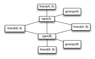
Figure 1: A sample ground network for a Markov Logic Network

Probabilistic Logic with Markov Logic Networks

To combine logical and probabilistic information, we utilize Markov Logic Networks (MLNs) [Richardson and Domingos (2006)]. MLNs are well suited for our approach since they provide an elegant framework for assigning weights to first-order logical rules, combining a diverse set of inference rules and performing sound probabilistic inference.

A weighted rule allows truth assignments in which not all instances of the rule hold. Equation 1 above shows sample weighted rules: Friends of ogres tend to be ogres and ogres tend to be grumpy. Suppose we have two constants, Anna ($A$) and Bob ($B$). Using these two constants and the predicate symbols in Equation 1, the set of all ground atoms we can construct is:

$$L_{A,B}=\{ ogre(A),ogre(B),grumpy(A),grumpy(B),friend(A,A),$$

$$friend(A,B),friend(B,A),friend(B,B)\}$$

If we only consider models over a domain with these two constants as entities, then each truth assignment to $L_{A,B}$ corresponds to a model. MLNs make the assumption of a one-to-one correspondence between constants in the system and entities in the domain. We discuss the effects of this domain closure assumption below.

Markov Networks or undirected graphical models [Pearl (1988)] compute the probability $P(X=x)$ of an assignment $x$ of values to the sequence $X$ of all variables in the model based on clique potentials, where a clique potential is a function that assigns a value to each clique (maximally connected subgraph) in the graph. Markov Logic Networks construct Markov Networks (hence their name) based on weighted first order logic formulas, like the ones in Equation 1. Figure 1 shows the network for Equation 1 with two constants. Every ground atom becomes a node in the graph, and two nodes are connected if they co-occur in a grounding of an input formula. In this graph, each clique corresponds to a grounding of a rule. For example, the clique including $friend(A,B)$, $ogre(A)$, and $ogre(B)$ corresponds to the ground rule $friend(A,B)\wedge ogre(A)\Rightarrow ogre(B)$. A variable assignment $x$ in this graph assigns to each node a value of either True or False, so it is a truth assignment (a world). The clique potential for the clique involving $friend(A,B)$, $ogre(A)$, and $ogre(B)$ is $\exp(1.1)$ if $x$ makes the ground rule true, and 0 otherwise. This allows for nonzero probability for worlds $x$ in which not all friends of ogres are also ogres, but it assigns exponentially more probability to a world for each ground rule that it satisfies.

More generally, an MLN takes as input a set of weighted first-order formulas $F=F_{1},\ldots,F_{n}$ and a set $C$ of constants, and constructs an undirected graphical model in which the set of nodes is the set of ground atoms constructed from $F$ and $C$. It computes the probability distribution $P(X=x)$ over worlds based on this undirected graphical model. The probability of a world (a truth assignment) $x$ is defined as:

$$P(X=x)=\dfrac{1}{Z}\exp\left(\sum_{i}{w_{i}n_{i}\left(x\right)}\right)$$ (3)

where $i$ ranges over all formulas $F_{i}$ in $F$, $w_{i}$ is the weight of $F_{i}$, $n_{i}(x)$ is the number of groundings of $F_{i}$ that are true in the world $x$, and $Z$ is the partition function (i.e., it normalizes the values to probabilities). So the probability of a world increases exponentially with the total weight of the ground clauses that it satisfies.

Below, we use $R$ (for rules) to denote the input set of weighted formulas. In addition, an MLN takes as input an evidence set $E$ asserting truth values for some ground clauses. For example, $ogre(A)$ means that Anna is an ogre. Marginal inference for MLNs calculates the probability $P(Q|E,R)$ for a query formula $Q$.

Alchemy [Kok et al. (2005)] is the most widely used MLN implementation. It is a software package that contains implementations of a variety of MLN inference and learning algorithms. However, developing a scalable, general-purpose, accurate inference method for complex MLNs is an open problem. MLNs have been used for various NLP applications including unsupervised coreference resolution [Poon and Domingos (2008)], semantic role labeling [Riedel and Meza-Ruiz (2008)] and event extraction [Riedel et al. (2009)].

Recognizing Textual Entailment

The task that we focus on in this paper is Recognizing Textual Entailment (RTE) [Dagan et al. (2013)], the task of determining whether one natural language text, the Text $T$, entails, contradicts, or is not related (neutral) to another, the Hypothesis $H$. “Entailment” here does not mean logical entailment: The Hypothesis is entailed if a human annotator judges that it plausibly follows from the Text. When using naturally occurring sentences, this is a very challenging task that should be able to utilize the unique strengths of both logic-based and distributional semantics. Here are examples from the SICK dataset [Marelli et al. (2014b)]:

• Entailment

• A man and a woman are walking together through the woods.

• A man and a woman are walking through a wooded area.

• Contradiction

• Nobody is playing the guitar

• A man is playing the guitar

• Neutral

• A young girl is dancing

• A young girl is standing on one leg

The SICK (“Sentences Involving Compositional Knowledge”) dataset, which we use for evaluation in this paper, was designed to foreground particular linguistic phenomena but to eliminate the need for world knowledge beyond linguistic knowledge. It was constructed from sentences from two image description datasets, ImageFlickr and the SemEval 2012 STS MSR-Video Description data. Randomly selected sentences from these two sources were first simplified to remove some linguistic phenomena that the dataset was not aiming to cover. Then additional sentences were created as variations over these sentences, by paraphrasing, negation, and reordering. RTE pairs were then created that consisted of a simplified original sentence paired with one of the transformed sentences (generated from either the same or a different original sentence).

We would like to mention two particular systems that were evaluated on SICK. The first is lai:semeval14 which was the top performing system at the original shared task. They use a linear classifier with many hand crafted features, including alignments, word forms, POS tags, distributional similarity, WordNet, and a unique feature called Denotational Similarity. Many of these hand crafted features are later incorporated in our lexical entailment classifier, described in section 5.2. The Denotational Similarity uses a large database of human- and machine-generated image captions to cleverly capture some world knowledge of entailments.

The second system is bjerva:2014semeval which also participated in the original SICK shared task, and achieved 81.6% accuracy. The RTE system uses Boxer to parse input sentences to logical form, then uses a theorem prover and a model builder to check for entailment and contradiction. The knowledge bases used are WordNet and PPDB. In contrast with our work, PPDB paraphrases are not translated to logical rules (section 5.3). Instead, in case a PPDB paraphrase rule applies to a pair of sentences, the rule is applied at the text level before parsing the sentence. Theorem provers and model builders have high precision detecting entailments and contradictions, but low recall. To improve recall, neutral pairs are reclassified using a set of textual, syntactic and semantic features.

3 System Overview

Figure 2: System Architecture

This section provides an overview of our system’s architecture, using the following RTE example to demonstrate the role of each component:

• A grumpy ogre is not smiling.

• A monster with a bad temper is not laughing.

Which in logic are:

• $\exists x.\>ogre(x)\wedge grumpy(x)\wedge\lnot\exists y.\>agent(y,x)\wedge smile(y)$

• $\exists x,y.\>monster(x)\wedge with(x,y)\wedge bad(y)\wedge temper(y)\wedge\lnot\exists z.\>agent(z,x)\wedge laugh(z)$.

This example needs the following rules in the knowledge base $KB$:

• laugh $\Rightarrow$ smile

• ogre $\Rightarrow$ monster

• grumpy $\Rightarrow$ with a bad temper

Figure 2 shows the high-level architecture of our system and Figure 3 shows the MLNs constructed by our system for the given RTE example.

$$D: \{O,L,C_{o}\}$$

$$G: \{ogre(O),grumpy(O),monster(O),agent(L,O),smile(L),laugh(L),$$

$$skolem_{f}(O,C_{o}),with(O,C_{o}),bad(C_{o}),temper(C_{o})\}$$

$$T: ogre(O)\wedge grumpy(O)\wedge\lnot\exists y.\>agent(y,O)\wedge smile(y)\>|\>\infty$$

$$r_{1}: \forall x.\>laugh(x)\Rightarrow smile(x)\>|\>w_{1}\times w_{ppdb}$$

$$r_{2}: \forall x.\>ogre(x)\Rightarrow monster(x)\>|\>w_{wn}=\infty$$

$$r_{3}: \forall x.\>grumpy(x)\Rightarrow\forall y.\>skolem_{f}(x,y)\Rightarrow with(x,y)\wedge bad(y)\wedge temper(y)\>|$$

$$\>w_{3}\times w_{eclassif}$$

$$sk: skolem_{f}(O,C_{o})\>|\>\infty$$

$$A: \forall x.\>agent(L,x)\wedge laugh(L)\>|\>1.5$$

$$H: \exists x,y.\>monster(x)\wedge with(x,y)\wedge bad(y)\wedge temper(y)\wedge\lnot\exists z.\>agent(z,x)\wedge laugh(z)$$

(a) MLN to calculate $P(H|T,KB,W_{T,H})$

$$D: \{O,C_{o},M,T\}$$

$$G: \{ogre(O),grumpy(O),monster(O),skolem_{f}(O,C_{o}),with(O,C_{o}),bad(C_{o}),$$

$$temper(C_{o}),monster(M),with(M,T),bad(T),temper(T)\}$$

$$T: ogre(O)\wedge grumpy(O)\wedge\lnot\exists y.\>agent(y,O)\wedge smile(y)\>|\>\infty$$

$$r_{1}: \forall x.\>laugh(x)\Rightarrow smile(x)\>|\>w_{1}\times w_{ppdb}$$

$$r_{2}: \forall x.\>ogre(x)\Rightarrow monster(x)\>|\>w_{wn}=\infty$$

$$r_{3}: \forall x.\>grumpy(x)\Rightarrow\forall y.\>skolem_{f}(x,y)\Rightarrow with(x,y)\wedge bad(y)\wedge temper(y)\>|$$

$$\>w_{3}\times w_{eclassif}$$

$$sk: skolem_{f}(O,C_{o})\>|\>\infty$$

$$A: monster(M)\wedge with(M,T)\wedge bad(T)\wedge temper(T)\>|\>1.5$$

$$\lnot H: \lnot\exists x,y.\>monster(x)\wedge with(x,y)\wedge bad(y)\wedge temper(y)\wedge\lnot\exists z.\>agent(z,x)\wedge laugh(z)$$

(b) MLN to calculate $P(\lnot H|T,KB,W_{T,\lnot H})$

Figure 3: MLNs for the given RTE example. The RTE task is represented as two inferences $P(H|T,KB,W_{T,H})$ and $P(\lnot H|T,KB,W_{T,\lnot H})$ (Section 4.1). $D$ is the set of constants in the domain. $T$ and $r_{3}$ are skolemized and $sk$ is the skolem function of $r_{3}$ (Section 4.2). $G$ is the set of non-False (True or unknown) ground atoms as determined by the CWA (Section 4.3, 6.2). $A$ is the CWA for the negated part of $H$ (Section 4.3). $D,G,A$ are the world assumptions $W_{T,H}$ ( or $W_{T,\lnot H}$). $r_{1},r_{2},r_{3}$ are the $KB$. $r_{1}$ and its weight $w_{1}$ are from PPDB (Section 5.3). $r_{2}$ is from WordNet (Section 5.3). $r_{3}$ is constructed using the Modified Robinson Resolution (Section 5.1), and its weight $w_{3}$ is calculated using the entailment rules classifier (Section 5.2). The resource specific weights $w_{ppdb},w_{eclassif}$ are learned using weight learning (Section 6.3). Finally the two probabilities are calculated using MLN inference where $H$ (or $\lnot H$) is the query formula (Section 6.1)

Our system has three main components:

1. Logical Representation (Section 4), where input natural sentences $T$ and $H$ are mapped into logic then used to represent the RTE task as a probabilistic inference problem.

2. Knowledge Base Construction $KB$ (Section 5), where the background knowledge is collected from different sources, encoded as first-order logic rules, weighted and added to the inference problem. This is where distributional information is integrated into our system.

3. Inference (Section 6), which uses MLNs to solve the resulting inference problem.

One powerful advantage of using a general-purpose probabilistic logic as a semantic representation is that it allows for a highly modular system. Therefore, the most recent advancements in any of the system components, in parsing, in knowledge base resources and distributional semantics, and in inference algorithms, can be easily incorporated into the system.

In the Logical Representation step (Section 4), we map input sentences $T$ and $H$ to logic. Then, we show how to map the three-way RTE classification (entailing, neutral, or contradicting) to probabilistic inference problems. The mapping of sentences to logic differs from standard first order logic in several respects because of properties of the probabilistic inference system. First, MLNs make the Domain Closure Assumption (DCA), which states that there are no objects in the universe other than the named constants [Richardson and Domingos (2006)]. This means that constants need to be explicitly introduced in the domain in order to make probabilistic logic produce the expected inferences. Another representational issue that we discuss is why we should make the closed-world assumption, and its implications on the task representation.

In the Knowledge Base Construction step $KB$ (Section 5), we collect inference rules from a variety of sources. We add rules from existing databases, in particular WordNet [Princeton University (2010)] and PPDB [Ganitkevitch, Van Durme, and Callison-Burch (2013)]. To integrate distributional semantics, we use a variant of Robinson resolution to align the Text $T$ and the Hypothesis $H$, and to find the difference between them, which we formulate as an entailment rule. We then train a lexical and phrasal entailment classifier to assess this rule. Ideally, rules need be contextualized to handle polysemy, but we leave that to future work.

In the Inference step (Section 6), automated reasoning for MLNs is used to perform the RTE task. We implement an MLN inference algorithm that directly supports querying complex logical formula, which is not supported in the available MLN tools [Beltagy and Mooney (2014)]. We exploit the closed-world assumption to help reduce the size of the inference problem in order to make it tractable [Beltagy and Mooney (2014)]. We also discuss weight learning for the rules in the knowledge base.

4 Logical Representation

The first component of our system parses sentences into logical form and uses this to represent the RTE problem as MLN inference. We start with Boxer [Bos (2008)], a rule-based semantic analysis system that translates a CCG parse into a logical form. The formula

$$\exists x,y,z.\>ogre(x)\wedge agent(y,x)\wedge love(y)\wedge patient(y,z)\wedge princess(z)$$ (4)

is an example of Boxer producing discourse representation structures using a neo-Davidsonian framework. We call Boxer’s output alone an “uninterpreted logical form” because the predicate symbols are simply words and do not have meaning by themselves. Their semantics derives from the knowledge base $KB$ we build in Section 5. The rest of this section discusses how we adapt Boxer output for MLN inference.

4.1 Representing Tasks as Text and Query

Representing Natural Language Understanding Tasks

In our framework, a language understanding task consists of a text and a query, along with a knowledge base. The text describes some situation or setting, and the query in the simplest case asks whether a particular statement is true of the situation described in the text. The knowledge base encodes relevant background knowledge: lexical knowledge, world knowledge, or both. In the textual entailment task, the text is the Text $T$, and the query is the Hypothesis $H$. The sentence similarity (STS) task can be described as two text/query pairs. In the first pair, the first sentence is the text and the second is the query, and in the second pair the roles are reversed [Beltagy, Erk, and Mooney (2014)]. In question answering, the input documents constitute the text and the query has the form $H(x)$ for a variable $x$; and the answer is the entity $e$ such that $H(e)$ has the highest probability given the information in $T$.

In this paper, we focus on the simplest form of text/query inference, which applies to both RTE and STS: Given a text $T$ and query $H$, does the text entail the query given the knowledge base $KB$? In standard logic, we determine entailment by checking whether $T\wedge KB\Rightarrow H$. (Unless we need to make the distinction explicitly, we overload notation and use the symbol $T$ for the logical form computed for the text, and $H$ for the logical form computed for the query.) The probabilistic version is to calculate the probability $P(H|T,KB,W_{T,H})$, where $W_{T,H}$ is a world configuration, which includes the size of the domain. We discuss $W_{T,H}$ in Sections 4.2 and 4.3. While we focus on the simplest form of text/query inference, more complex tasks such as question answering still have the probability $P(H|T,KB,W_{T,H})$ as part of their calculations.

Representing Textual Entailment

RTE asks for a categorical decision between three categories, Entailment, Contradiction, and Neutral. A decision about Entailment can be made by learning a threshold on the probability $P(H|T,KB,W_{T,H})$. To differentiate between Contradiction and Neutral, we additionally calculate the probability $P(\lnot H|T,KB,W_{T,\lnot H})$. If $P(H|T,KB,W_{T,H})$ is high while $P(\lnot H|T,KB,W_{T,\lnot H})$ is low, this indicates entailment. The opposite case indicates contradiction. If the two probabilities values are close, this means $T$ does not significantly affect the probability of $H$, indicating a neutral case. To learn the thresholds for these decisions, we train an SVM classifier with LibSVM’s default parameters [Chang and Lin (2001)] to map the two probabilities to the final decision. The learned mapping is always simple and reflects the intuition described above.

4.2 Using a Fixed Domain Size

MLNs compute a probability distribution over possible worlds, as described in Section 2. When we describe a task as a text $T$ and a query $H$, the worlds over which the MLN computes a probability distribution are “mini-worlds”, just large enough to describe the situation or setting given by $T$. The probability $P(H|T,KB,W_{T,H})$ then describes the probability that $H$ would hold given the probability distribution over the worlds that possibly describe $T$. The use of “mini-worlds” is by necessity, as MLNs can only handle worlds with a fixed domain size, where “domain size” is the number of constants in the domain. (In fact, this same restriction holds for all current practical probabilistic inference methods, including PSL [Bach et al. (2013)].)

Formally, the influence of the set of constants on the worlds considered by an MLN can be described by the Domain Closure Assumption (DCA, [Genesereth and Nilsson (1987), Richardson and Domingos (2006)]): The only models considered for a set $F$ of formulas are those for which the following three conditions hold: (a) Different constants refer to different objects in the domain, (b) the only objects in the domain are those that can be represented using the constant and function symbols in $F$, and (c) for each function $f$ appearing in $F$, the value of $f$ applied to every possible tuple of arguments is known, and is a constant appearing in $F$. Together, these three conditions entail that there is a one-to-one relation between objects in the domain and the named constants of $F$. When the set of all constants is known, it can be used to ground predicates to generate the set of all ground atoms, which then become the nodes in the graphical model. Different constant sets result in different graphical models. If no constants are explicitly introduced, the graphical model is empty (no random variables).

This means that to obtain an adequate representation of an inference problem consisting of a text $T$ and query $H$, we need to introduce a sufficient number of constants explicitly into the formula: The worlds that the MLN considers need to have enough constants to faithfully represent the situation in $T$ and not give the wrong entailment for the query $H$. In what follows, we explain how we determine an appropriate set of constants for the logical-form representations of $T$ and $H$. The domain size that we determine is one of the two components of the parameter $W_{T,H}$.

Skolemization

We introduce some of the necessary constants through the well-known technique of Skolemization (Skolem, 1920). It transforms a formula $\forall x_{1}\ldots x_{n}\exists y.F$ to $\forall x_{1}\ldots x_{n}.F^{*}$, where $F^{*}$ is formed from $F$ by replacing all free occurrences of $y$ in $F$ by a term $f(x_{1},\ldots,x_{n})$ for a new function symbol $f$. If $n=0$, f is called a Skolem constant, otherwise a Skolem function. Although Skolemization is a widely used technique in first-order logic, it is not frequently employed in probabilistic logic since many applications do not require existential quantifiers.

We use Skolemization on the text $T$ (but not the query $H$, as we cannot assume a priori that it is true). For example, the logical expression in Equation 4, which represents the sentence T: An ogre loves a princess, will be Skolemized to:

$$ogre(O)\wedge agent(L,O)\wedge love(L)\wedge patient(L,N)\wedge princess(N)$$ (5)

where $O,L,N$ are Skolem constants introduced into the domain.

Standard Skolemization transforms existential quantifiers embedded under universal quantifiers to Skolem functions. For example, for the text T: All ogres snore and its logical form $\forall x.\>ogre(x)\Rightarrow\exists y.\>agent(y,x)\wedge snore(y)$ the standard Skolemization is $\forall x.\>ogre(x)\Rightarrow agent(f(x),x)\wedge snore(f(x))$. Per condition (c) of the DCA above, if a Skolem function appeared in a formula, we would have to know its value for any constant in the domain, and this value would have to be another constant. To achieve this, we introduce a new predicate $Skolem_{f}$ instead of each Skolem function $f$, and for every constant that is an ogre, we add an extra constant that is a loving event. The example above then becomes:

$$\begin{gathered}T:\forall x.\>ogre(x)\Rightarrow\forall y.\>Skolem_{f}(x,y)\Rightarrow agent(y,x)\wedge snore(y)\end{gathered}$$

If the domain contains a single ogre $O_{1}$, then we introduce a new constant $C_{1}$ and an atom $Skolem_{f}(O_{1},C_{1})$ to state that the Skolem function $f$ maps the constant $O_{1}$ to the constant $C_{1}$.

Existence

But how would the domain contain an ogre $O_{1}$ in the case of the text T: All ogres snore, $\forall x.ogre(x)\Rightarrow\exists y.agent(y,x)\wedge snore(y)$? Skolemization does not introduce any variables for the universally quantified $x$. We still introduce a constant $O_{1}$ that is an ogre. This can be justified by pragmatics since the sentence presupposes that there are, in fact, ogres (Strawson, 1950; Geurts, 2007). We use the sentence’s parse to identify the universal quantifier’s restrictor and body, then introduce entities representing the restrictor of the quantifier (Beltagy and Erk, 2015). The sentence T: All ogres snore effectively changes to T: All ogres snore, and there is an ogre. At this point, Skolemization takes over to generate a constant that is an ogre. Sentences like T: There are no ogres is a special case: For such sentences, we do not generate evidence of an ogre. In this case, the non-emptiness of the domain is not assumed because the sentence explicitly negates it.

Universal quantifiers in the query

The most serious problem with the DCA is that it affects the behavior of universal quantifiers in the query. Suppose we know that T: Shrek is a green ogre, represented with Skolemization as $ogre(SH)\wedge green(SH)$. Then we can conclude that H: All ogres are green, because by the DCA we are only considering models with this single constant which we know is both an ogre and green. To address this problem, we again introduce new constants.

We want a query H: All ogres are green to be judged true iff there is evidence that all ogres will be green, no matter how many ogres there are in the domain. So $H$ should follow from $T_{2}$: All ogres are green but not from $T_{1}$: There is a green ogre. Therefore we introduce a new constant $D$ for the query and assert $ogre(D)$ to test if we can then conclude that $green(D)$. The new evidence $ogre(D)$ prevents the query from being judged true given $T_{1}$. Given $T_{2}$, the new ogre $D$ will be inferred to be green, in which case we take the query to be true. Again, with a query such as H: There are no ogres, we do not generate any evidence for the existence of an ogre.

4.3 Setting Prior Probabilities

Suppose we have an empty text $T$, and the query H: A is an ogre, where $A$ is a constant in the system. Without any additional information, the worlds in which $ogre(A)$ is true are going to be as likely as the worlds in which the ground atom is false, so $ogre(A)$ will have a probability of 0.5. So without any text $T$, ground atoms have a prior probability in MLNs that is not zero. This prior probability depends mostly on the size of the set $F$ of input formulas. The prior probability of an individual ground atom can be influenced by a weighted rule, for example $ogre(A)\mid-3$, with a negative weight, sets a low prior probability on $A$ being an ogre. This is the second group of parameters that we encode in $W_{T,H}$: weights on ground atoms to be used to set prior probabilities.

Prior probabilities are problematic for our probabilistic encoding of natural language understanding problems. As a reminder, we probabilistically test for entailment by computing the probability of the query given the text, or more precisely $P(H|T,KB,W_{T,H})$. However, how useful this conditional probability is as an indication of entailment depends on the prior probability of $H$, $P(H|KB,W_{T,H})$. For example, if $H$ has a high prior probability, then a high conditional probability $P(H|T,KB,W_{T,H})$ does not add much information because it is not clear if the probability is high because $T$ really entails $H$, or because of the high prior probability of $H$. In practical terms, we would not want to say that we can conclude from T: All princesses snore that H: There is an ogre just because of a high prior probability for the existence of ogres.

To solve this problem and make the probability $P(H|T,KB,W_{T,H})$ less sensitive to $P(H|KB,W_{T,H})$, we pick a particular $W_{T,H}$ such that the prior probability of $H$ is approximately zero, $P(H|KB,W_{T,H})\approx 0$, so that we know that any increase in the conditional probability is an effect of adding $T$. For the task of RTE, where we need to distinguish Entailment, Neutral, and Contradiction, this inference alone does not account for contradictions, which is why an additional inference $P(\lnot H|T,KB,W_{T,\lnot H})$ is needed.

For the rest of this section, we show how to set the world configurations $W_{T,H}$ such that $P(H|KB,W_{T,H})\approx 0$ by enforcing the closed-world assumption (CWA). This is the assumption that all ground atoms have very low prior probability (or are false by default).

Using the CWA to set the prior probability of the query to zero

The closed-world assumption (CWA) is the assumption that everything is false unless stated otherwise. We translate it to our probabilistic setting as saying that all ground atoms have very low prior probability. For most queries $H$, setting the world configuration $W_{T,H}$ such that all ground atoms have low prior probability is enough to achieve that $P(H|KB,W_{T,H})\approx 0$ (not for negated $H$s, and this case is discussed below). For example, H: An ogre loves a princess, in logic is:

$$\begin{gathered}H:\exists x,y,z.\>ogre(x)\wedge agent(y,x)\wedge love(y)\wedge patient(y,z)\wedge princess(z)\end{gathered}$$

Having low prior probability on all ground atoms means that the prior probability of this existentially quantified $H$ is close to zero.

We believe that this setup is more appropriate for probabilistic natural language entailment for the following reasons. First, this aligns with our intuition of what it means for a query to follow from a text: that $H$ should be entailed by $T$ not because of general world knowledge. For example, if T: An ogre loves a princess, and H: Texas is in the USA, then although $H$ is true in the real world, $T$ does not entail $H$. Another example: T: An ogre loves a princess, H: An ogre loves a green princess, again, $T$ does not entail $H$ because there is no evidence that the princess is green, in other words, the ground atom $green(N)$ has very low prior probability.

The second reason is that with the CWA, the inference result is less sensitive to the domain size (number of constants in the domain). In logical forms for typical natural language sentences, most variables in the query are existentially quantified. Without the CWA, the probability of an existentially quantified query increases as the domain size increases, regardless of the evidence. This makes sense in the MLN setting, because in larger domains the probability that something exists increases. However, this is not what we need for testing natural language queries, as the probability of the query should depend on $T$ and $KB$, not the domain size. With the CWA, what affects the probability of $H$ is the non-zero evidence that $T$ provides and $KB$, regardless of the domain size.

The third reason is computational efficiency. As discussed in Section 2, Markov Logic Networks first compute all possible groundings of a given set of weighted formulas which can require significant amounts of memory. This is particularly striking for problems in natural language semantics because of long formulas. beltagy:starai14 show how to utilize the CWA to address this problem by reducing the number of ground atoms that the system generates. We discuss the details in Section 6.2.

Setting the prior probability of negated $H$ to zero

While using the CWA is enough to set $P(H|KB,W_{T,H})\approx 0$ for most $H$s, it does not work for negated $H$ (negation is part of $H$). Assuming that everything is false by default and that all ground atoms have very low prior probability (CWA) means that all negated queries $H$ are true by default. The result is that all negated $H$ are judged entailed regardless of $T$. For example, T: An ogre loves a princess would entail H: No ogre snores. This $H$ in logic is:

$$\begin{gathered}H:\forall x,y.\>ogre(x)\Rightarrow\lnot(agent(y,x)\wedge snore(y))\end{gathered}$$

As both $x$ and $y$ are universally quantified variables in $H$, we generate evidence of an ogre $ogre(O)$ as described in section 4.2. Because of the CWA, $O$ is assumed to be does not snore, and $H$ ends up being true regardless of $T$.

To set the prior probability of $H$ to $\approx 0$ and prevent it from being assumed true when $T$ is just uninformative, we construct a new rule $A$ that implements a kind of anti-CWA. $A$ is formed as a conjunction of all the predicates that were not used to generate evidence before, and are negated in $H$. This rule $A$ gets a positive weight indicating that its ground atoms have high prior probability. As the rule $A$ together with the evidence generated from $H$ states the opposite of the negated parts of $H$, the prior probability of $H$ is low, and $H$ cannot become true unless $T$ explicitly negates $A$. $T$ is translated into unweighted rule, which are taken to have infinite weight, and which thus can overcome the finite positive weight of $A$. Here is a Neutral RTE example, T: An ogre loves a princess, and H: No ogre snores. Their representations are:

• $\exists x,y,z.\>ogre(x)\wedge agent(y,x)\wedge love(y)\wedge patient(y,z)\wedge princess(z)$

• $\forall x,y.\>ogre(x)\Rightarrow\lnot(agent(y,x)\wedge snore(y))$

• $ogre(O)$

• $agent(S,O)\wedge snore(S)|w=1.5$

$E$ is the evidence generated for the universally quantified variables in $H$, and $A$ is the weighted rule for the remaining negated predicates. The relation between $T$ and $H$ is Neutral, as $T$ does not entail $H$. This means, we want $P(H|T,KB,W_{T,H})\approx 0$, but because of the CWA, $P(H|T,KB,W_{T,H})\approx 1$. Adding $A$ solves this problem and $P(H|T,A,KB,W_{T,H})\approx 0$ because $H$ is not explicitly entailed by $T$.

In case $H$ contains existentially quantified variables that occur in negated predicates, they need to be universally quantified in $A$ for $H$ to have a low prior probability. For example, H: There is an ogre that is not green:

$$\begin{gathered}H:\exists x.\>ogre(x)\wedge\lnot green(x)\\ A:\forall x.\>green(x)|w=1.5\end{gathered}$$

If one variable is universally quantified and the other is existentially quantified, we need to do something more complex. Here is an example, H: An ogre does not snore:

$$\begin{gathered}H:\exists x.\>ogre(x)\wedge\lnot(\>\exists y.\>agent(y,x)\wedge snore(y)\>)\\ A:\forall v.\>agent(S,v)\wedge snore(S)|w=1.5\end{gathered}$$

Notes about how inference proceeds with the rule $A$ added

If $H$ is a negated formula that is entailed by $T$, then $T$ (which has infinite weight) will contradict $A$, allowing $H$ to be true. Any weighted inference rules in the knowledge base $KB$ will need weights high enough to overcome $A$. So the weight of $A$ is taken into account when computing inference rule weights.

In addition, adding the rule $A$ introduces constants in the domain that are necessary for making the inference. For example, take T: No monster snores, and H: No ogre snores, which in logic are:

• $\lnot\exists x,y.\>monster(x)\wedge agent(y,x)\wedge snore(y)$

• $\lnot\exists x,y.\>ogre(x)\wedge agent(y,x)\wedge snore(y)$

• $ogre(O)\wedge agent(S,O)\wedge snore(S)|w=1.5$

• $\forall x.\>ogre(x)\Rightarrow monster(x)$

Without the constants $O$ and $S$ added by the rule $A$, the domain would have been empty and the inference output would have been wrong. The rule $A$ prevents this problem. In addition, the introduced evidence in $A$ fit the idea of “evidence propagation” mentioned above, (detailed in Section 6.2). For entailing sentences that are negated, like in the example above, the evidence propagates from $H$ to $T$ (not from $T$ to $H$ as in non-negated examples). In the example, the rule $A$ introduces an evidence for $ogre(O)$ that then propagates from the LHS to the RHS of the $KB$ rule.

4.4 Textual Entailment and Coreference

The adaptations of logical form that we have discussed so far apply to any natural language understanding problem that can be formulated as text/query pairs. The adaptation that we discuss now is specific to textual entailment. It concerns coreference between text and query.

For example, if we have T: An ogre does not snore and H: An ogre snores, then strictly speaking $T$ and $H$ are not contradictory because it is possible that the two sentences are referring to different ogres. Although the sentence uses an ogre not the ogre, the annotators make the assumption that the ogre in $H$ refers to the ogre in $T$. In the SICK textual entailment dataset, many of the pairs that annotators have labeled as contradictions are only contradictions if we assume that some expressions corefer across $T$ and $H$.

For the above examples, here are the logical formulas with coreference in the $updated\>\lnot H$:

$$T :\exists x.\>ogre(x)\wedge\lnot(\exists y.\>agent(y,x)\wedge snore(y))$$

$$Skolemized\>T :ogre(O)\wedge\lnot(\exists y.\>agent(y,O)\wedge snore(y))$$

$$H :\exists x,y.\>ogre(x)\wedge agent(y,x)\wedge snore(y)$$

$$\lnot H :\lnot\exists x,y.\>ogre(x)\wedge agent(y,x)\wedge snore(y)$$

$$updated\>\lnot H :\lnot\exists y.\>ogre(O)\wedge agent(y,O)\wedge snore(y)$$

Notice how the constant $O$ representing the ogre in $T$ is used in the $updated\>\lnot H$ instead of the quantified variable $x$.

We use a rule-based approach to determining coreference between $T$ and $H$, considering both coreference between entities and coreference of events. Two items (entities or events) corefer if they 1) have different polarities, and 2) share the same lemma or share an inference rule. Two items have different polarities in $T$ and $H$ if one of them is embedded under a negation and the other is not. For the example above, ogre in $T$ is not negated, and ogre in $\lnot H$ is negated, and both words are the same, so they corefer.

A pair of items in $T$ and $H$ under different polarities can also corefer if they share an inference rule. In the example of T: A monster does not snore and H: An ogre snores, we need monster and ogre to corefer. For cases like this, we rely on the inference rules found using the modified Robinson resolution method discussed in Section 5.1. In this case, it determines that monster and ogre should be aligned, so they are marked as coreferring. Here is another example: T: An ogre loves a princess, H: An ogre hates a princess. In this case, loves and hates are marked as coreferring.

4.5 Using multiple parses

In our framework that uses probabilistic inference followed by a classifier that learns thresholds, we can easily incorporate multiple parses to reduce errors due to misparsing. Parsing errors lead to errors in the logical form representation, which in turn can lead to erroneous entailments. If we can obtain multiple parses for a text $T$ and query $H$, and hence multiple logical forms, this should increase our chances of getting a good estimate of the probability of $H$ given $T$.

The default CCG parser that Boxer uses is C&C  Clark and Curran (2004). This parser can be configured to produce multiple ranked parses Ng and Curran (2012); however, we found that the top parses we get from C&C are usually not diverse enough and map to the same logical form. Therefore, in addition to the top C&C parse, we use the top parse from another recent CCG parser, EasyCCG Lewis and Steedman (2014).

So for a natural language text $N_{T}$ and query $N_{H}$, we obtain two parses each, say $S_{T1}$ and $S_{T2}$ for $T$ and $S_{H1}$ and $S_{H2}$ for $H$, which are transformed to logical forms $T_{1},T_{2},H_{1},H_{2}$. We now compute probabilities for all possible combinations of representations of $N_{T}$ and $N_{H}$: the probability of $H_{1}$ given $T_{1}$, the probability of $H_{1}$ given $T_{2}$, and conversely also the probabilities of $H_{2}$ given either $T_{1}$ or $T_{2}$. If the task is textual entailment with three categories Entailment, Neutral, and Contradiction, then as described in Section 4.1 we also compute the probability of $\lnot H_{1}$ given either $T_{1}$ or $T_{2}$, and the probability of $\lnot H_{1}2$ given either $T_{1}$ or $T_{2}$. When we use multiple parses in this manner, the thresholding classifier is simply trained to take in all of these probabilities as features. In Section 7, we evaluate using C&C alone and using both parsers.

5 Knowledge Base Construction

This section discusses the automated construction of the knowledge base, which includes the use of distributional information to predict lexical and phrasal entailment. This section integrates two aims that are conflicting to some extent, as alluded to in the introduction. The first is to show that a general-purpose in-depth natural language understanding system based on both logical form and distributional representations can be adapted to perform the RTE task well enough to achieve state of the art results. To achieve this aim, we build a classifier for lexical and phrasal entailment that includes many task-specific features that have proven effective in state-of-the-art systems Marelli et al. (2014a); Bjerva et al. (2014); Lai and Hockenmaier (2014). The second aim is to provide a framework in which we can test different distributional approaches on the task of lexical and phrasal entailment as a building block in a general textual entailment system. To achieve this second aim, in Section 7) we provide an in-depth ablation study and error analysis for the effect of different types of distributional information within the lexical and phrasal entailment classifier.

Since the biggest computational bottleneck for MLNs is the creation of the network, we do not want to add a large number of inference rules blindly to a given text/query pair. Instead, we first examine the text and query to determine inference rules that are potentially useful for this particular entailment problem. For pre-existing rule collections, we add all possibly matching rules to the inference problem (Section 5.3). For more flexible lexical and phrasal entailment, we use the text/query pair to determine additionally useful inference rules, then automatically create and weight these rules. We use a variant of Robinson resolution Robinson (1965) to compute the list of useful rules (Section 5.1), then apply a lexical and phrasal entailment classifier (Section 5.2) to weight them.

Ideally, the weights that we compute for inference rules should depend on the context in which the words appear. After all, the ability to take context into account in a flexible fashion is one of the biggest advantages of distributional models. Unfortunately the textual entailment data that we use in this paper does not lend itself to contextualization – polysemy just does not play a large role in any of the existing RTE datasets that we have used so far. Therefore, we leave this issue to future work.

5.1 Robinson Resolution for Alignment and Rule Extraction

To avoid undo complexity in the MLN, we only want to add inference rules specific to a given text $T$ and query $H$. Earlier versions of our system generated distributional rules matching any word or short phrase in $T$ with any word or short phrase in $H$. This includes many unnecessary rules, for example for T: An ogre loves a princess and H: A monster likes a lady, the system generates rules linking ogre to lady. In this paper, we use a novel method to generate only rules directly relevant to $T$ and $H$: We assume that $T$ entails $H$, and ask what missing rule set $KB$ is necessary to prove this entailment. We use a variant of Robinson resolution Robinson (1965) to generate this $KB$. Another way of viewing this technique is that it generates an alignment between words and phrases in $T$ and words or phrases in $H$ guided by the logic.

Modified Robinson Resolution

Robinson resolution is a theorem proving method for testing unsatisfiability that has been used in some previous RTE systems Bos:09. It assumes a formula in conjunctive normal form (CNF), a conjunction of clauses, where a clause is a disjunction of literals, and a literal is a negated or non-negated atom. More formally, the formula has the form $\forall x_{1},\ldots,x_{n}\big{(}C_{1}\wedge\ldots\wedge C_{m})$, where $C_{j}$ is a clause and it has the form $L_{1}\vee\ldots\vee L_{k}$ where $L_{i}$ is a literal, which is an atom $a_{i}$ or a negated atom $\lnot a_{i}$. The resolution rule takes two clauses containing complementary literals, and produces a new clause implied by them. Writing a clause $C$ as the set of its literals, we can formulate the rule as:

$$\frac{C_{1}\cup\{L_{1}\}~{}~{}~{}~{}~{}~{}~{}~{}C_{2}\cup\{L_{2}\}}{(C_{1}\cup C_{2})_{\theta}}$$

where $\theta$ is a most general unifier of $L_{1}$ and $\neg L_{2}$.

In our case, we use a variant of Robinson resolution to remove the parts of text $T$ and query $H$ that the two sentences have in common. Instead of one set of clauses, we use two: one is the CNF of $T$, the other is the CNF of $\neg H$. The resolution rule is only applied to pairs of clauses where one clause is from $T$, the other from $H$. When no further applications of the resolution rule are possible, we are left with remainder formulas $rT$ and $rH$. If $rH$ contains the empty clause, then $H$ follows from $T$ without inference rules. Otherwise, inference rules need to be generated. In the simplest case, we form a single inference rule as follows. All variables occurring in $rT$ or $rH$ are existentially quantified, all constants occurring in $rT$ or $rH$ are un-Skolemized to new universally quantified variables, and we infer the negation of $rH$ from $rT$. That is, we form the inference rule

$$\forall x_{1}\ldots x_{n}\exists y_{1}\ldots y_{m}.\>rT\overline{\theta}\Rightarrow\lnot rH\overline{\theta}$$

where $\{y_{1}\ldots y_{m}\}$ is the set of all variables occurring in $rT$ or $rH$, $\{a_{1},\ldots a_{n}\}$ is the set of all constants occurring in $rT$ or $rH$ and $\overline{\theta}$ is the inverse of a substitution $\theta:\{a_{1}\to x_{1},\ldots,a_{n}\to x_{n}\}$ for distinct variables $x_{1},\ldots,x_{n}$.

For example, consider T: An ogre loves a princess and H: A monster loves a princess. This gives us the following two clause sets. Note that all existential quantifiers have been eliminated through Skolemization. The query is negated, so we get five clauses for $T$ but only one for $H$.

$$\begin{array}[]{rl}T:&\{ogre(A)\},\{princess(B)\},\{love(C\},\{agent(C,A)\},\{patient(C,B)\}\\ \neg H:&\{\neg monster(x),\neg princess(y),\neg love(z),\neg agent(z,x),\neg patient(z,y)\}\end{array}$$

The resolution rule can be applied 4 times. After that, $C$ has been unified with $z$ (because we have resolved $love(C)$ with $love(z)$), $B$ with $y$ (because we have resolved $princess(B)$ with $princess(y)$), and $A$ with $x$ (because we have resolved $agent(C,A)$ with $agent(z,x)$). The formula $rT$ is $ogre(A)$, and $rH$ is $\neg monster(A)$. So the rule that we generate is:

$$\forall x.ogre(x)\Rightarrow monster(x)$$

The modified Robinson resolution thus does two things at once: It removes words that $T$ and $H$ have in common, leaving the words for which inference rules are needed, and it aligns words and phrases in $T$ with words and phrases in $H$ through unification.

One important refinement to this general idea is that we need to distinguish content predicates that correspond to content words (nouns, verb and adjectives) in the sentences from non-content predicates such as Boxer’s meta-predicates $agent(X,Y)$. Resolving on non-content predicates can result in incorrect rules, for example in the case of T: A person solves a problem and H: A person finds a solution to a problem, in CNF:

$$\begin{array}[]{rl}T:&\{person(A)\},\{solve(B)\},\{problem(C)\},\{agent(B,A)\},\{patient(B,C)\}\\ \neg H:&\{\neg person(x),\neg find(y),\neg solution(z),\neg problem(u),\neg agent(y,x),\neg patient(y,z),\\ &\neg to(z,u)\}\end{array}$$

If we resolve $patient(B,C)$ with $patient(y,z)$, we unify the problem $C$ with the solution $z$, leading to a wrong alignment. We avoid this problem by resolving on non-content predicates only when they are fully grounded (that is, when the substitution of variables with constants has already been done by some other resolution step involving content predicates).

In this variant of Robinson resolution, we currently do not perform any search, but unify two literals only if they are fully grounded or if the literal in $T$ has a unique literal in $H$ that it can be resolved with, and vice versa. This works for most pairs in the SICK dataset. In future work, we would like to add search to our algorithm, which will help produce better rules for sentences with duplicate words.

Rule Refinement

The modified Robinson resolution algorithm gives us one rule per text/query pair. This rule needs postprocessing, as it is sometimes too short (omitting relevant context), and often it combines what should be several inference rules.

In many cases, a rule needs to be extended. This is the case when it only shows the difference between text and query is too short and needs context to be usable as a distributional rule, for example: T: A dog is running in the snow, H: A dog is running through the snow, the rule we get is $\forall x,y.\>in(x,y)\Rightarrow through(x,y)$. Although this rule is correct, it does not carry enough information to compute a meaningful vector representation for each side. What we would like instead is a rule that infers “run through snow” from “run in snow”.

Remember that the variables $x$ and $y$ were Skolem constants in $rT$ and $rH$, for example $rT:in(R,S)$ and $rH:through(R,S)$. We extend the rule by adding the content words that contain the constants $R$ and $S$. In this case, we add the running event and the snow back in. The final rule is: $\forall x,y.\>run(x)\wedge in(x,y)\wedge snow(y)\Rightarrow run(x)\wedge through(x,y)\wedge snow(y)$.

In some cases however, extending the rule adds unnecessary complexity. However, we have no general algorithm for when to extend a rule, which would have to take context into account. At this time, we extend all rules as described above. As discussed below, the entailment rules subsystem can itself choose to split long rules, and it may choose to split these extended rules again.

Sometimes, long rules need to be split. A single pair $T$ and $H$ gives rise to one single pair $rT$ and $rH$, which often conceptually represents multiple inference rules. So we split $rT$ and $rH$ as follows. First, we split each formula into disconnected sets of predicates. For example, consider T: The doctors are healing a man, H: The doctor is helping the patient which leads to the rule $\forall x,y.\>heal(x)\wedge man(y)\Rightarrow help(x)\wedge patient(y)$. The formula $rT$ is split into $heal(x)$ and $man(y)$ because the two literals do not have any variable in common and there is no relation (such as $agent()$) to link them. Similarly, $rH$ is split into $help(x)$ and $patient(y)$. If any of the splits has more than one verb, we split it again, where each new split contains one verb and its arguments.

After that, we create new rules that link any part of $rT$ to any part of $rH$ with which it has at least one variable in common. So for our example we get $\forall x\>heal(x)\Rightarrow help(x)$ and $\forall y\>man(y)\Rightarrow patient(y)$.

There are cases where splitting the rule does not work, for example with A person, who is riding a bike $\Rightarrow$ A biker . Here, splitting the rule and using person $\Rightarrow$ biker loses crucial context information. So we do not perform those additional splits at the level of the logical form, though the entailment rules subsystem may choose to do further splits.

Rules as training data

The output from the previous steps is a set of rules $\{r_{1},...,r_{n}\}$ for each pair $T$ and $H$. One use of these rules is to test whether $T$ probabilistically entails $H$. But there is a second use too: The lexical and phrasal entailment classifier that we describe below is a supervised classifier, which needs training data. So we use the training part of the SICK dataset to create rules through modified Robinson resolution, which we then use to train the lexical and phrasal entailment classifier. For simplicity, we translate the Robinson resolution rules into textual rules by replacing each Boxer predicate with its corresponding word.

Computing inference-rule training data from RTE data requires deriving labels for individual rules from the labels on RTE pairs (Entailment, Contradiction and Neutral). The Entailment cases are the most straightforward. Knowing that $T\wedge r_{1}\wedge...\wedge r_{n}\Rightarrow H$, then it must be that all $r_{i}$ are entailing. We automatically label all $r_{i}$ of the entailing pairs as entailing rules.

For Neutral pairs, we know that $T\wedge r_{1}\wedge...\wedge r_{n}\nRightarrow H$, so at least one of the $r_{i}$ is non-entailing. We experimented with automatically labeling all $r_{i}$ as non-entailing, but that adds a lot of noise to the training data. For example, if T: A man is eating an apple and H: A guy is eating an orange, then the rule man $\Rightarrow$ guy is entailing, but the rule apple $\Rightarrow$ orange is non-entailing. So we automatically compare the $r_{i}$ from a Neutral pair to the entailing rules derived from entailing pairs. All rules $r_{i}$ found among the entailing rules from entailing pairs are assumed to be entailing (unless $n=1$, that is, unless we only have one rule), and all other rules are assumed to be non-entailing. We found that this step improved the accuracy of our system. To further improve the accuracy, we performed a manual annotation of rules derived from Neutral pairs, focusing only on the rules that do not appear in Entailing. We labeled rules as either entailing or non-entailing. From around 5,900 unique rules, we found 737 to be entailing. In future work, we plan to use multiple instance learning Dietterich, Lathrop, and Lozano-Perez (1997); Bunescu and Mooney (2007) to avoid manual annotation; we discuss this further in Section 8.

For Contradicting pairs, we make a few simplifying assumptions that fit almost all such pairs in the SICK dataset. In most of the contradiction pairs in SICK, one of the two sentences $T$ or $H$ is negated. For pairs where $T$ or $H$ has a negation, we assume that this negation is negating the whole sentence, not just a part of it. We first consider the case where $T$ is not negated, and $H=\lnot S_{h}$. As $T$ contradicts $H$, it must hold that $T\Rightarrow\lnot H$, so $T\Rightarrow\lnot\lnot S_{h}$, and hence $T\Rightarrow S_{h}$. This means that we just need to run our modified Robinson resolution with the sentences $T$ and $S_{h}$ and label all resulting $r_{i}$ as entailing.

Next we consider the case where $T=\lnot S_{t}$ while $H$ is not negated. As $T$ contradicts $H$, it must hold that $\lnot S_{t}\Rightarrow\lnot H$, so $H\Rightarrow S_{t}$. Again, this means that we just need to run the modified Robinson resolution with $H$ as the “Text” and $S_{t}$ as the “Hypothesis” and label all resulting $r_{i}$ as entailing.

The last case of contradiction is when both $T$ and $H$ are not negated, for example: T: A man is jumping into an empty pool, H: A man is jumping into a full pool, where empty and full are antonyms. As before, we run the modified Robinson resolution with $T$ and $H$ and get the resulting $r_{i}$. Similar to the Neutral pairs, at least one of the $r_{i}$ is a contradictory rule, while the rest could be entailing or contradictory rules. As for the Neutral pairs, we take a rule $r_{i}$ to be entailing if it is among the entailing rules derived so far. All other rules are taken to be contradictory rules. We did not do the manual annotation for these rules because they are few.

5.2 The Lexical and Phrasal Entailment Rule Classifier

After extracting lexical and phrasal rules using our modified Robinson resolution (Section 5.1), we use several combinations of distributional information and lexical resources to build a lexical and phrasal entailment rule classifier (entailment rule classifier for short) for weighting the rules appropriately. These extracted rules create an especially valuable resource for testing lexical entailment systems, as they contain a variety of entailment relations (hypernymy, synonymy, antonymy, etc.), and are actually useful in an end-to-end RTE system.

We describe the entailment rule classifier in multiple parts. In Section 5.2.1, we overview a lexical entailment rule classifier, which only handles single words. Section 5.2.2 describes the lexical resources used. In Section 5.2.3, we describe how our previous work in supervised hypernymy detection is used in the system. In Section 5.2.4, we describe the approaches for extending the classifier to handle phrases.

5.2.1 Lexical Entailment Rule Classifier

We begin by describing the lexical entailment rule classifier, which only predicts entailment between single words, treating the task as a supervised classification problem given the lexical rules constructed from the modified Robinson resolution as input. We use numerous features which we expect to be predictive of lexical entailment. Many were previously shown to be successful for the SemEval 2014 Shared Task on lexical entailment Marelli et al. (2014a); Bjerva et al. (2014); Lai and Hockenmaier (2014). Altogether, we use four major groups of features as summarized in Table 1 and described in detail below.

Name	Description	Type	#
Wordform			18
Same word	Same lemma, surface form	Binary	2
POS	POS of LHS, POS of RHS, same POS	Binary	10
Sg/Pl	Whether LHS/RHS/both are singular/plural	Binary	6
WordNet			18
OOV	True if a lemma is not in WordNet, or no path exists	Binary	1
Hyper	True if LHS is hypernym of RHS	Binary	1
Hypo	True if RHS is hypernym of LHS	Binary	1
Syn	True if LHS and RHS is in same synset	Binary	1
Ant	True if LHS and RHS are antonyms	Binary	1
Path Sim	Path similarity (NLTK)	Real	1
Path Sim Hist	Bins of path similarity (NLTK)	Binary	12
Distributional features (Lexical)			28
OOV	True if either lemma not in dist space	Binary	2
BoW Cosine	Cosine between LHS and RHS in BoW space	Real	1
Dep Cosine	Cosine between LHS and RHS in Dep space	Real	1
BoW Hist	Bins of BoW Cosine	Binary	12
Dep Hist	Bins of Dep Cosine	Binary	12
Asymmetric Features Roller, Erk, and Boleda (2014)			600
Diff	LHS dep vector $-$ RHS dep vector	Real	300
DiffSq	RHS dep vector $-$ RHS dep vector, squared	Real	300

Table 1: List of features in the lexical entailment classifier, along with types and counts

Wordform Features We extract a number of simple features based on the usage of the LHS and RHS in their original sentences. We extract features for whether the LHS and RHS have the same lemma, same surface form, same POS, which POS tags they have, and whether they are singular or plural. Plurality is determined from the POS tags.

WordNet Features We use WordNet 3.0 to determine whether the LHS and RHS have known synonymy, antonymy, hypernymy, or hyponymy relations. We disambiguate between multiple synsets for a lemma by selecting the synsets for the LHS and RHS which minimize their path distance. If no path exists, we choose the most common synset for the lemma. Path similarity, as implemented in the Natural Language Toolkit Bird, Klein, and Loper (2009), is also used as a feature.

Distributional Features We measure distributional similarity in two distributional spaces, one which models topical similarity (BoW), and one which models syntactic similarity (Dep). We use cosine similarity of the LHS and RHS in both spaces as features.

One very important feature set used from distributional similarity is the histogram binning of the cosines. We create 12 additional binary, mutually-exclusive features, which mark whether the distributional similarity is within a given range. We use the ranges of exactly 0, exactly 1, 0.01-0.09, 0.10-0.19, …, 0.90-0.99. Figure 4 shows the importance of these histogram features: words that are very similar (0.90-0.99) are much less likely to be entailing than words which are moderately similar (0.70-0.89). This is because the most highly similar words are likely to be cohyponyms.

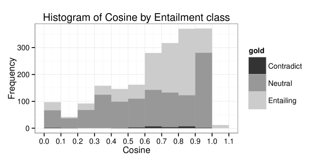
Figure 4: Distribution of entailment relations on lexical items by cosine. Highly similar pairs (0.90-0.99) are less likely entailing than moderately similar pairs (0.70-0.89).

5.2.2 Preparing Distributional Spaces

As described in the previous section, we use distributional semantic similarity as features for the entailment rules classifier. Here we describe the preprocessing steps to create these distributional resources.

Corpus and Preprocessing: We use the BNC, ukWaC and a 2014-01-07 copy of Wikipedia. All corpora are preprocessed using Stanford CoreNLP. We collapse particle verbs into a single token, and all tokens are annotated with a (short) POS tag so that the same lemma with a different POS is modeled separately. We keep only content words (NN, VB, RB, JJ) appearing at least 1000 times in the corpus. The final corpus contains 50,984 types and roughly 1.5B tokens.

Bag-of-Words vectors: We filter all but the 51k chosen lemmas from the corpus, and create one sentence per line. We use Skip-Gram Negative Sampling to create vectors Mikolov et al. (2013). We use 300 latent dimensions, a window size of 20, and 15 negative samples. These parameters were not tuned, but chosen as reasonable defaults for the task. We use the large window size to ensure the BoW vectors captured more topical similarity, rather than syntactic similarity, which is modeled by the dependency vectors.

Dependency vectors: We extract (lemma/POS, relation, context/POS) tuples from each of the Stanford Collapsed CC Dependency graphs. We filter tuples with lemmas not in our 51k chosen types. Following typeDM, we model inverse relations and mark them separately. For example, “red/JJ car/NN” will generate tuples for both (car/NN, amod, red/JJ) and (red/JJ, amod^-1, car/NN). After extracting tuples, we discard all but the top 100k (relation, context/POS) pairs and build a vector space using lemma/POS as rows, and (relation, context/POS) as columns. The matrix is transformed with Positive Pointwise Mutual Information (PPMI), and reduced to 300 dimensions using Singular Value Decomposition (SVD). We do not vary these parameters, but chose them as they performed best in prior work Roller, Erk, and Boleda (2014).

5.2.3 Asymmetric Entailment Features

As an additional set of features, we also use the representation previously employed by the asymmetric, supervised hypernymy classifier described by roller:coling14. Previously, this classifier was only used on artificial datasets, which encoded specific lexical relations, like hypernymy, co-hyponymy, and meronymy. Here, we use its representation to encode just the three general relations: entailment, neutral, and contradiction.

The asymmetric features take inspiration from mikolov:2013naacl, who found that differences between distributional vectors often encode certain linguistic regularities, like $\vec{king}-\vec{man}+\vec{woman}\approx\vec{queen}$. In particular the asymmetric classifier uses two sets of features, $<f,g>$, where:

$$f_{i}(LHS,RHS) =\vec{LHS}_{i}-\vec{RHS}_{i}$$

$$g_{i}(LHS,RHS) =f_{i}^{2},$$

that is, the vector difference between the LHS and the RHS, and this difference vector squared. Both feature sets are extremely important to strong performance.

For these asymmetric features, we use the Dependency space described earlier. We choose the Dep space because we previously found that spaces reduced using SVD outperform word embeddings generated by the Skip-gram procedure. We do not use both spaces, because of the large number of features this creates.

Recently, there have been considerable work in detecting lexical entailments using only distributional vectors. The classifiers proposed by fu:acl:2014; levy:2015tt; and kruszewski2015deriving could have also been used in place of these asymmetric features, but we reserve evaluations of these models for future work.

5.2.4 Extending Lexical Entailment to Phrases

The lexical entailment rule classifier described in previous sections is limited to only simple rules, where the LHS and RHS are both single words. Many of the rules generated by the modified Robinson resolution are actually phrasal rules, such as little boy $\rightarrow$ child, or running $\rightarrow$ moving quickly. In order to model these phrases, we use two general approaches: first, we use a state-of-the-art compositional model, in order to create vector representations of phrases, and then include the same similarity features described in the previous section. The full details of the compositional distributional model are described in Section 5.2.5.

In addition to a compositional distributional model, we also used a simple, greedy word aligner, similar to the one described by lai:semeval14. This aligner works by finding the pair of words on the LHS and RHS which are most similar in a distributional space, and marking them as “aligned”. The process is repeated until at least one side is completely exhausted. For example, “red truck $\rightarrow$ big blue car”, we would align “truck” with “car” first, then “red” with “blue”, leaving “big” unaligned.

After performing the phrasal alignment, we compute a number of base features, based on the results of the alignment procedure. These include values like the length of the rule, the percent of words unaligned, etc. We also compute all of the same features used in the lexical entailment rule classifier (Wordform, WordNet, Distributional) and compute their min/mean/max across all the alignments. We do not include the asymmetric entailment features as the feature space then becomes extremely large. Table 2 contains a listing of all phrasal features used.

Name	Description	Type	#
Base			9
Length	Length of rules	Real	2
Length Diff	Length of LHS - length of RHS	Real	1
Aligned	Number of alignments	Real	1
Unaligned	Number of unaligned words on LHS, RHS	Real	2
Pct aligned	Percentage of words aligned	Real	1
Pct unaligned	Percentage of words unaligned on LHS, RHS	Real	2
Distributional features Paperno, Pham, and Baroni (2014)			16
Cosine	Cosine between mean constituent vectors	Real	1
Hist	Bins of cosine between mean constituent vectors	Binary	12
Stats	Min/mean/max between constituent vectors	Real	3
Lexical features of aligned words			192
Wordform	Min/mean/max of each Wordform feature		54
WordNet	Min/mean/max of each WordNet feature		54
Distributional	Min/mean/max of each Distributional feature		84

Table 2: Features used in Phrasal Entailment Classifier, along with types and counts.

5.2.5 Phrasal Distributional Semantics

We build phrasal distributional space based on the practical lexical function model of paperno:acl14. We again use as the corpus a concatenation of BNC, ukWaC and English Wikipedia, parsed with the Stanford CoreNLP parser. We focus on 5 types of dependency labels, “amod”, “nsubj”, “dobj”, “pobj”, “acomp”, and combine the governor and dependent words of these dependencies to form adjective-noun, subject-verb, verb-object, preposition-noun and verb-complement phrases respectively. We only retain phrases where both the governor and the dependent are among the 50K most frequent words in the corpus, resulting in 1.9 million unique phrases. The co-occurrence counts of the 1.9 million phrases with the 20K most frequent neighbor words in a 2-word window are converted to a PPMI matrix, and reduced to 300 dimensions by performing SVD on a lexical space and applying the resulting representation to the phrase vectors, normalized to length 1.

Paperno et al. represent a word as a vector, which represents the contexts in which the word can appear, along with a number of matrices, one for each type of dependent that the word can take. For a transitive verb like chase, this would be one matrix for subjects, and one for direct objects. The representation of the phrase chases dog is then

$$\vec{chase}+\mathop{chase}^{\Box_{o}}\times\vec{dog}$$

where $\times$ is matrix multiplication, and when the phrase is extended with cat to form cat chases dog, the representation is

$$\vec{chase}+\mathop{chase}^{\Box_{s}}\times\vec{cat}+(\vec{chase}+\mathop{chase}^{\Box_{o}}\times\vec{dog})$$

For verbs, the practical lexical function model trains a matrix for each of the relations nsubj, dobj and acomp, for adjectives a matrix for amod, and for prepositions a matrix for pobj. For example, the amod matrix of the adjective “red/JJ” is trained as follows. We collect all phrases in which “red/JJ” serves as adjective modifier (assuming the number of such phrases is $N$), like “red/JJ car/NN”, “red/JJ house/NN” etc., and construct two $300\times N$ matrices $M_{arg}$ and $M_{ph}$, where the $i$th column of $M_{arg}$ is the vector of the noun modified by “red/JJ” in the $i$th phrase ($\overrightarrow{car},\overrightarrow{house}$, etc.), and the $i$th column of $M_{ph}$ is vector of phrase $i$ minus the vector of “red/JJ” ($\overrightarrow{red\ car}-\overrightarrow{red},\overrightarrow{red\ house}-\overrightarrow{red}$, etc.), normalized to length 1. Then the amod matrix $\mathop{red}^{\Box(amod)}\in R^{300\times 300}$ of “red/JJ” can be computed via ridge regression. Given trained matrices, we compute the composition vectors by applying the functions recursively starting from the lowest dependency.

As discussed above, some of the logical rules from Section 5.1 need to be split into multiple rules. We use the dependency parse to split long rules by iteratively searching for the highest nodes in the dependency tree that occur in the logical rule, and identifying the logical rule words that are its descendants in phrases that the practical lexical functional model can handle. After splitting, we perform greedy alignment on phrasal vectors to pair up rule parts. Similar to Section 5.2.4, we iteratively identify the pair of phrasal vectors on the LHS and RHS which have the highest cosine similarity until one side has no more phrases.

5.3 Precompiled Rules

The second group of rules is collected from existing databases. We collect rules from WordNet Princeton University (2010) and the paraphrase collection PPDB Ganitkevitch, Van Durme, and Callison-Burch (2013). We use simple string matching to find the set of rules that are relevant to a given text/query pair $T$ and $H$. If the left-hand side of a rule is a substring of $T$ and the right-hand is a substring of $H$, the rule is added, and likewise for rules with LHS in $H$ and RHS in $T$. Rules that go from $H$ to $T$ are important in case $T$ and $H$ are negated, e.g. $T$: No ogre likes a princess, $H$: No ogre loves a princess. The rule needed is love $\Rightarrow$ like which goes from $H$ to $T$.

WordNet

WordNet Princeton University (2010) is a lexical database of words grouped into sets of synonyms. In addition to grouping synonyms, it lists semantic relations connecting groups. We represent the information on WordNet as “hard” logical rules. The semantic relations we use are:

• Synonymy: $\forall x.\>man(x)\Leftrightarrow guy(x)$

• Hypernymy: $\forall x.\>car(x)\Rightarrow vehicle(x)$

• Antonymy: $\forall x.\>tall(x)\Leftrightarrow\lnot short(x)$

One advantage of using logic is that it is a powerful representation that can effectively represent these different semantic relations.

Paraphrase collections

Paraphrase collections are precompiled sets of rules, e.g: a person riding a bike $\Rightarrow$ a biker. We translate paraphrase collections, in this case PPDB Ganitkevitch, Van Durme, and Callison-Burch (2013), to logical rules. We use the Lexical, One-To-Many and Phrasal sections of the XL version of PPDB.

We use a simple rule-based approach to translate natural-language rules to logic. First, we can make the assumption that the translation of a PPDB rule is going to be a conjunction of positive atoms. PPDB does contain some rules that are centrally about negation, such as deselected $\Rightarrow$ not selected, but we skip those as the logical form analysis already handles negation. As always, we want to include in $KB$ only rules pertaining to a particular text/query pair $T$ and $H$. Say $LHS\Rightarrow RHS$ is a rule such that $LHS$ is a substring of $T$ and $RHS$ is a substring of $H$. Then each word in $LHS$ gets represented by a unary predicate applied to a variable, and likewise for $RHS$ – note that we can expect the same predicates to appear in the logical forms $L(T)$ and $L(H)$ of the text and query. For example, if the rule is a person riding a bike $\Rightarrow$ a biker, then we get the atoms $person(p)$, $riding(r)$ and $bike(b)$ for the $LHS$, with variables $p,r,b$. We then add Boxer meta-predicates to the logical form for $LHS$, and likewise for $RHS$. Say that $L(T)$ includes $person(A)\wedge ride(B)\wedge bike(C)\wedge agent(B,A)\wedge patient(B,C)$ for constants $A$, $B$, and $C$, then we extend the logical form for $LHS$ with $agent(r,p)\wedge patient(r,b)$. We proceed analogously for $RHS$. This gives us the logical forms: $L(LHS)=person(p)\wedge agent(r,p)\wedge riding(r)\wedge patient(r,b)\wedge bike(b)$ and $L(RHS)=biker(k)$.

The next step is to bind the variables in $L(LHS)$ to those in $L(RHS)$. In the example above, the variable $k$ in the $RHS$ should be matched with the variable $p$ in the $LHS$. We determine these bindings using a simple rule-based approach: We manually define paraphrase rule templates for PPDB, which specify variable bindings. A rule template is conditioned on the part-of-speech tags of the words involved. In our example it is $N_{1}V_{2}N_{3}\Rightarrow N_{1}$, which binds the variables of the first $N$ on the left to the first $N$ on the right, unifying the variables $p$ and $k$. The final paraphrase rule is: $\forall p,r,b.\>person(p)\wedge agent(r,p)\wedge riding(r)\wedge patient(r,b)\wedge bike(b)\Rightarrow biker(p)$. In case some variables in the $RHS$ remain unbound, they are existentially quantified, e.g.: $\forall p.\>pizza(p)\Rightarrow\exists q.\>slice(p)\wedge of(p,q)\wedge pizza(q)$.

Each PPDB rule comes with a set of similarity scores which we need to map to a single MLN weight. We use the simple log-linear equation suggested by ganitkevitch:naacl13 to map the scores into a single value:

$$weight(r)=-\sum^{N}_{i=1}\lambda_{i}\log\varphi_{i}$$ (6)

where, $r$ is the rule, $N$ is number of the similarity scores provided for the rule $r$, $\varphi_{i}$ is the value of the $i$th score, and $\lambda_{i}$ is its scaling factor. For simplicity, following  ganitkevitch:naacl13, we set all $\lambda_{i}$ to 1. To map this weight to a final MLN rule weight, we use the weight-learning method discussed in Section 6.3.

Handcoded rules

We also add a few handcoded rules to the $KB$ that we do not get from other resources. For the SICK dataset, we only add several lexical rules where one side of the rule is the word nobody, e.g: nobody $\Leftrightarrow\lnot$ somebody and nobody $\Leftrightarrow\lnot$ person.

6 Probabilistic Logical Inference

We now turn to the last of the three main components of our system, probabilistic logical inference. MLN inference is usually intractable, and using MLN implementations “out of the box” does not work for our application. This section discusses an MLN implementation that supports complex queries and uses the closed world assumption (CWA) to decrease problem size, hence making inference more efficient. Finally, this section discusses a simple weight learning scheme to learn global scaling factors for weighted rules in $KB$ from different sources.

6.1 Complex formulas as queries

Current implementations of MLNs like Alchemy Kok et al. (2005) do not allow queries to be complex formulas, they can only calculate probabilities of ground atoms. This section discusses an inference algorithm for arbitrary query formulas.

The standard work-around

Although current MLN implementations can only calculate probabilities of ground atoms, they can be used to calculate the probability of a complex formula through a simple work-around. The complex query formula $H$ is added to the MLN using the hard formula:

$$H\Leftrightarrow result(D)\>|\>\infty$$ (7)

where $result(D)$ is a new ground atom that is not used anywhere else in the MLN. Then, inference is run to calculate the probability of $result(D)$, which is equal to the probability of the formula $H$. However, this approach can be very inefficient for the most common form of queries, which are existentially quantified queries, e.g:

$$H:\>\exists x,y,z.\>ogre(x)\wedge agent(y,x)\wedge love(y)\wedge patient(y,z)\wedge princess(z)$$ (8)

Grounding of the backward direction of the double-implication is very problematic because the existentially quantified formula is replaced with a large disjunction over all possible combinations of constants for variables $x,y$ and $z$ Gogate and Domingos (2011). Converting this disjunction to clausal form becomes increasingly intractable as the number of variables and constants grow.

New inference method

Instead, we propose an inference algorithm to directly calculate the probability of complex query formulas. In MLNs, the probability of a formula is the sum of the probabilities of the possible worlds that satisfy it. gogate:uai11 show that to calculate the probability of a formula $H$ given a probabilistic knowledge base $KB$, it is enough to compute the partition function $Z$ of $KB$ with and without $H$ added as a hard formula:

$$P(H\mid KB)=\frac{Z(KB\cup\{(H,\infty)\})}{Z(KB)}$$ (9)

Therefore, all we need is an appropriate algorithm to estimate the partition function $Z$ of a Markov network. Then, we construct two ground networks, one with the query and one without, and estimate their $Z$s using that estimator. The ratio between the two $Z$s is the probability of $H$.

We use SampleSearch Gogate and Dechter (2011) to estimate the partition function. SampleSearch is an importance sampling algorithm that has been shown to be effective when there is a mix of probabilistic and deterministic (hard) constraints, a fundamental property of the inference problems we address. Importance sampling in general is problematic in the presence of determinism, because many of the generated samples violate the deterministic constraints, and they get rejected. Instead, SampleSearch uses a base sampler to generate samples then uses backtracking search with a SAT solver to modify the generated sample if it violates the deterministic constraints. We use an implementation of SampleSearch that uses a generalized belief propagation algorithm called Iterative Join-Graph Propagation (IJGP) Dechter, Kask, and Mateescu (2002) as a base sampler. This version is available online Gogate (2014).

For cases like the example $H$ in Equation 8, we need to avoid generating a large disjunction because of the existentially quantified variables. So we replace $H$ with its negation $\ \lnot H$, replacing the existential quantifiers with universals, which are easier to ground and perform inference upon. Finally, we compute the probability of the query $P(H)=1-P(\lnot H)$. Note that replacing $H$ with $\ \lnot H$ cannot make inference with the standard work-around faster, because with $\ \lnot H$, the direction $\lnot H\Rightarrow result(D)$ suffers from the same problem of existential quantifiers that we previously had with $H\Leftarrow result(D)$.

6.2 Inference Optimization using the Closed-World Assumption

This section explains why our MLN inference problems are computationally difficult, then explains how the closed-world assumption (CWA) can be used to reduce the problem size and speed up inference. For more details, see beltagy:starai14.

In the inference problems we address, formulas are typically long, especially the query $H$. The number of ground clauses of a first-order formula is exponential in the number of variables in the formula, it is $O(c^{v})$, where $c$ is number of constants in the domain and $v$ is number of variables in the formula. For a moderately long formula, the number of resulting ground clauses is infeasible to process.

We have argued above (Section 4.3) that for probabilistic inference problems based on natural language text/query pairs, it makes sense to make the closed world assumption: If we want to know if the query is true in the situation or setting laid out in the text, we should take as false anything not said in the text. In our probabilistic setting, the CWA amounts to giving low prior probabilities to all ground atoms unless they can be inferred from the text and knowledge base. However, we found that a large fraction of the ground atoms cannot be inferred from the text and knowledge base, and their probabilities remain very low. As an approximation, we can assume that this small probability is exactly zero and these ground atoms are false, without significantly affecting the probability of the query. This will remove a large number of the ground atoms, which will dramatically decrease the size of the ground network and speed up inference.

We assume that all ground atoms are false by default unless they are can be inferred from the text and the knowledge base $T\wedge KB$. For example:

$$T: ogre(O)\wedge agent(S,O)\wedge snore(S)$$

$$KB: \forall x.\>ogre(x)\Rightarrow monster(x)$$

$$H: \exists x,y.\>monster(x)\wedge agent(y,x)\wedge snore(y)$$

Ground atoms $\{ogre(O),snore(S),agent(S,O)\}$ are not false because they can be inferred from $T$. Ground atom $monster(O)$ is also not false because it can be inferred from $T\wedge KB$. All other ground atoms are false.

Here is an example of how this simplifies the query $H$. $H$ is equivalent to a disjunction of all its possible groundings: $H:\>(monster(O)\wedge agent(S,O)\wedge snore(S))\vee(monster(O)\wedge agent(O,O)\wedge snore(O))\vee(monster(S)\wedge agent(O,S)\wedge snore(O))\vee(monster(S)\wedge agent(S,S)\wedge snore(S))$. Setting all ground atoms to false except the inferred ones, then simplifying the expression, we get: $H:\>monster(O)\wedge agent(S,O)\wedge snore(S)$. Notice that most ground clauses of $H$ are removed because they are False. We are left just with the ground clauses that potentially have a non-zero probability. Dropping all False ground clauses leaves an exponentially smaller number of ground clauses in the ground network. Even though the inference problem remains exponential in principle, the problem is much smaller in practice, such that inference becomes feasible. In our experiments with the SICK dataset, the number of ground clauses for the query ranges from 0 to 19,209 with mean 6. This shows that the CWA effectively reduces the number of ground clauses for the query from millions (or even billions) to a manageable number. With the CWA, the average number of inferrable ground atoms (ignoring ground atoms from the text) ranges from 0 to 245 with an average of 18.

6.3 Weight Learning

We use weighted rules from different sources, both PPDB weights (Section 5.3) and the confidence of the entailments rule classifier (Section 5.2). These weights are not necessarily on the same scale, for example one source could produce systematically larger weights than the other. To map them into uniform weights that can be used within an MLN, we use weight learning. Similar to the work of zirn:ijcnlp11, we learn a single mapping parameter for each source of rules that functions as a scaling factor:

$$MLNweight=scalingFactor\times ruleWeight$$ (10)

We use a simple grid search to learn the scaling factors that optimize performance on the RTE training data.

Assuming that all rule weights are in $[0,1]$ (this is the case for classification confidence scores, and PPDB weights can be scaled), we also try the following mapping:

$$MLNweight=scalingFactor\times\log(\frac{ruleWeight}{1-ruleWeight})$$ (11)

This function assures that for an MLN with a single rule $LHS\Rightarrow RHS\>|\>MLNweight$, it is the case that $P(RHS|LHS)=ruleWeight$, given that $scalingFactor=1$.

7 Evaluation

This section evaluates our system. First, we evaluate several lexical and phrasal distributional systems on the rules that we collected using modified Robinson resolution. This includes an in-depth analysis of different types of distributional information within the entailment rule classifier. Second, we use the best configuration we find in the first step as a knowledge base and evaluate our system on the RTE task using the SICK dataset.

Dataset: The SICK dataset, which is described in Section 2, consists of 5,000 pairs for training and 4,927 for testing. Pairs are annotated for RTE and STS (Semantic Textual Similarity) tasks. We use the RTE annotations of the dataset.

7.1 Evaluating the Entailment Rule Classifier

The entailment rule classifier described in Section 5.2 constitutes a large portion of the full system’s end-to-end performance, but consists of many different feature sets providing different kinds of information. In this section, we thoroughly evaluate the entailment rule classifier, both quantitatively and qualitatively, to identify the individual and holistic value of each feature set and systematic patterns. However, this evaluation may also be used as a framework by future lexical semantics research to see its value in end-to-end textual entailment systems. For example, we could have also included features corresponding to the many measures of distributional inclusion which were developed to predict hypernymy Weeds, Weir, and McCarthy (2004); Kotlerman et al. (2010); Lenci and Benotto (2012); Santus (2013), or other supervised lexical entailment classifiers Baroni et al. (2012); Fu et al. (2014); Weeds et al. (2014); Levy et al. (2015); Kruszewski, Paperno, and Baroni (2015).

Evaluation is broken into four parts: first, we overview performance of the entire entailment rule classifier on all rules, both lexical and phrasal. We then break down these results into performance on only lexical rules and only phrasal rules. Finally, we look at only the asymmetric features to address concerns raised by levy:2015tt. In all sections, we evaluate the lexical rule classifier on its ability to generalize to new word pairs, as well as the full system’s performance when the entailment rule classifier is used as the only source of knowledge.

Overall, we find that distributional semantics is of vital importance to the lexical rule classifier and the end-to-end system, especially when word relations are not explicitly found in WordNet. The introduction of syntactic distributional spaces and cosine binning are especially valuable, and greatly improve performance over our own prior work. Contrary to levy:2015tt, we find the asymmetric features provide better detection of hypernymy over memorizing of prototypical hypernyms, but the prototype vectors better capture examples which occur very often in the data; explicitly using both does best. Finally, we find, to our surprise, that a state-of-the-art compositional distributional method Paperno, Pham, and Baroni (2014) yields disappointing performance on phrasal entailment detection, though it does successfully identify non-entailments deriving from changing prepositions or semantic roles.

7.1.1 Experimental Setup

We use the gold standard annotations described in Section 5.1. We perform 10 fold cross-validation on the annotated training set, using the same folds in all settings. Since some RTE sentence pairs require multiple lexical rules, we ensure that cross-validation folds are stratified across the sentences, so that the same sentence cannot appear in both training and testing. We use a Logistic Regression classifier with an L2 regularizer. Since we perform three-way classification, we train models using one-vs-all.

Performance is measured in two main metrics. Intrinsic accuracy measures how the classifier performs in the cross-validation setting on the training data. This corresponds to treating lexical and phrasal entailment as a basic supervised learning problem. RTE accuracy is accuracy on the end task of textual entailment using the predictions of the entailment rule classifier. For RTE accuracy, the predictions of the entailment rule classifier were used as the only knowledge base in the RTE system. RTE training accuracy uses the predictions from the cross-validation experiment, and for RTE test accuracy the entailment rule classifier was trained on the whole training set.

7.1.2 Overall Lexical and Phrasal Entailment Evaluation

Table 3 shows the results of the Entailment experiments on all rules, both lexical and phrasal. In order to give bounds on our system’s performance, we present baseline score (entailment rule classifier always predicts non-entailing) and ceiling score (entailment rule classifier always predicts gold standard annotation).

Feature set	Intrinsic	RTE Train	RTE Test
Always guess neutral	64.3	73.9	73.3
Gold standard annotations	100.0	95.0	95.5
Base only	64.3	73.8	73.4
Wordform only	67.3	77.0	76.7
WordNet only	75.1	81.9	81.3
Dist (Lexical) only	71.5	78.7	77.7
Dist (Phrasal) only	66.9	75.9	75.1
Asym only	70.1	77.3	77.2
All features	79.9	84.0	83.0

Table 3: Cross-validation accuracy on Entailment on all rules

The ceiling score (entailment rule classifier always predicts gold standard annotation) does not achieve perfect performance. This is due to a number of different issues including misparses, imperfect rules generated by the modified Robinson resolution, a few system inference timeouts, and various idiosyncrasies of the SICK dataset.

Another point to note is that WordNet is by far the strongest set of features for the task. This is unsurprising, as synonymy and hypernymy information from WordNet gives nearly perfect information for much of the task. There are some exceptions, such as woman $\nrightarrow$ man, or black $\nrightarrow$ white, which WordNet lists as antonyms, but which are not considered contradictions in the SICK dataset (e.g: “T: A man is cutting a tomato” and “H: A woman is cutting a tomato” is not a contradiction). However, even though WordNet has extremely high coverage on this particular dataset, it still is far from exhaustive: about a quarter of the rules have at least one pair of words for which WordNet relations could not be determined.

The lexical distributional features do surprisingly well on the task, obtaining a test accuracy of 77.7 (Table 3). This indicates that, even with only distributional similarity, we do well enough to score in the upper half of systems in the original SemEval shared task, where the median test accuracy of all teams was 77.1 Marelli et al. (2014a). Two components were critical to the increased performance over our own prior work: first, the use of multiple distributional spaces (one topical, one syntactic); second, the binning of cosine values. While using only the BoW cosine similarity as a feature, the classifier actually performs below baseline (50.0 intrinsic accuracy; compare to Table 4). Similarly, only using syntactic cosine similarity as a feature also performs poorly (47.2 IA). However adding binning to either improves performance (64.3 and 64.7 for BoW and Dep), and adding binning to both improves it further (68.8 IA, as reported in Table 4).

The phrasal distributional similarity features, which are based on the state-of-the-art paperno:acl14 compositional vector space, perform somewhat disappointingly on the task. We discuss possible reasons for this below in Section 7.1.4.

We also note that the Basic Alignment features and WordForm features (described in Tables 1 and 2) do not do particularly well on their own. This is encouraging, as it means the dataset cannot be handled by simply expecting the same words to appear on the LHS and RHS. Finally, we note that the features are highly complementary, and the combination of all features gives a substantial boost to performance.

7.1.3 Evaluating the Lexical Entailment Rule Classifier

Table 4 shows performance of the classifier on only the lexical rules, which have single words on the LHS and RHS. In these experiments we use the same procedure as before, but omit the phrasal rules from the dataset. On the RTE tasks, we compute accuracy over only the SICK pairs which require at least one lexical rule. Note that a new ceiling score is needed, as some rules require both lexical and phrasal predictions, but we do not predict any phrasal rules.

Feature set	Intrinsic	RTE Train	RTE Test
Always guess neutral	56.6	69.4	69.3
Gold standard annotations	100.0	93.2	94.6
Wordform only	57.4	70.4	70.9
WordNet only	79.1	83.1	84.2
Dist (Lexical) only	68.8	76.3	76.7
Asym only	76.8	78.3	79.2
All features	84.6	82.7	83.8

Table 4: Cross-validation accuracy on Entailment on lexical rules only

Again we see that WordNet features have the highest contribution. Distributional rules still perform better than the baseline, but the gap between distributional features and WordNet is much more apparent. Perhaps most encouraging is the very high performance of the Asymmetric features: by themselves, they perform substantially better than just the distributional features. We investigate this further below in Section 7.1.5.

As with the entire dataset, we once again see that all the features are highly complementary, and intrinsic accuracy is greatly improved by using all the features together. It may be surprising that these significant gains in intrinsic accuracy do not translate to improvements on the RTE tasks; in fact, there is a minor drop from using all features compared to only using WordNet. This most likely depends on which pairs the system gets right or wrong. For sentences involving multiple lexical rules, errors become disproportionately costly. As such, the high-precision WordNet predictions are slightly better on the RTE task.

In a qualitative analysis comparing a classifier with only cosine distributional features to a classifier with the full feature set, we found that, as expected, the distributional features miss many hypernyms and falsely classify many co-hyponyms as entailing: We manually analyzed a sample of 170 pairs that the distributional classifier falsely classifies as entailing. Of these, 67 were co-hyponyms (39%), 33 were antonyms (19%), and 32 were context-specific pairs like stir/fry. On the other hand, most (87%) cases of entailment that the distributional classifier detects but the all-features classifier misses are word pairs that have no link in WordNet. These pairs include note $\to$ paper, swimmer $\to$ racer, eat $\to$ bite, and stand $\to$ wait.

7.1.4 Evaluating the Phrasal Entailment Rule Classifier

Table 5 shows performance when looking at only the phrasal rules. As with the evaluation of lexical rules, we evaluate the RTE tasks only on sentence pairs that use phrasal rules, and do not provide any lexical inferences. As such, the ceiling score must again be recomputed.

Feature set	Intrinsic	RTE Train	RTE Test
Always guess neutral	67.8	72.5	72.7
Gold standard annotations	100.0	91.9	92.8
Base only	68.3	73.3	73.6
Wordform only	72.5	77.1	77.1
WordNet only	73.9	78.3	77.7
Dist (Lexical) only	72.9	77.0	76.5
Dist (Phrasal) only	71.9	75.7	75.3
All features	77.8	79.7	78.8

Table 5: Cross-validation accuracy on Entailment on phrasal rules only

We first notice that the phrasal subset is generally harder than the lexical subset: none of the features sets on their own provide dramatic improvements over the baseline, or come particularly close to the ceiling score. On the other hand, using all features together does better than any of the feature groups by themselves, indicating again that the feature groups are highly complementary.

Distributional features perform rather close to the Wordform features, suggesting that possibly the Distributional features may simply be proxies for the same lemma and same POS features. A qualitative analysis comparing the predictions of Wordform and Distributional features shows otherwise though: the Wordform features are best at correctly identifying non-entailing phrases (higher precision), while the distributional features are best at correctly identifying entailing phrases (higher recall).

As with the full dataset, we see that the features based on paperno:acl14 do not perform as well as just the alignment-based distributional lexical features; in fact, they do not perform even as well as features which make predictions using only Wordform features. We qualitatively compare the Paperno et al. features (or phrasal features for short) to the features based on word similarity of greedily aligned words (or alignment features). We generally find the phrase features are much more likely to predict neutral, while the alignment-based features are much more likely to predict entailing. In particular, the phrasal vectors seem to be much better at capturing non-entailment based on differences in prepositions (walk inside building $\nrightarrow$ walk outside building), additional modifiers on the RHS (man $\nrightarrow$ old man, room $\nrightarrow$ darkened room), and changing semantic roles (man eats near kitten $\nrightarrow$ kitten eats). Surprisingly, we found the lexical distributional features were better at capturing complex paraphrases, such as teenage $\rightarrow$ in teens, ride bike $\rightarrow$ biker, or young lady $\rightarrow$ teenage girl.

7.1.5 Evaluating the Asymmetric Classifier

levy:2015tt show several experiments suggesting that asymmetric classifiers do not perform better at the task of identifying hypernyms than when the RHS vectors alone are used as features. That is, they find that the asymmetric classifier and variants frequently learn to identify prototypical hypernyms rather than the hypernymy relation itself. We look at our data in the light of the Levy et al. study, in particular as none of the entailment problem sets used by Levy et al. were derived from an existing RTE dataset.

In a qualitative analysis comparing the predictions of a classifier using only Asymmetric features with a classifier using only cosine similarity, we found that the Asymmetric classifier does substantially better at distinguishing hypernymy from co-hyponymy. This is what we had hoped to find, as we had previously found an Asymmetric classifier to perform well at identifying hypernymy in other data Roller, Erk, and Boleda (2014), and cosine is known to heavily favor co-hyponymy Baroni and Lenci (2011). However, we also find that cosine features are better at discovering synonymy, and that Asymmetric frequently mistakes antonymy as an entailing. We did a quantitative analysis comparing the predictions of a classifier using only Asymmetric features to a classifier that tries to learn typical hyponyms or hypernyms by using only the LHS vectors, or the RHS vectors, or both. Table 6 shows the results of these experiments.

Feature set	Intrinsic	RTE Train	RTE Test
Always guess neutral	56.6	69.4	69.3
Gold standard annotations	100.0	93.2	94.6
Asym only	76.8	78.3	79.2
LHS only	65.4	73.8	73.5
RHS only	73.2	78.6	79.9
LHS + RHS	76.4	79.8	80.6
Asym + LHS + RHS	81.4	81.4	82.6

Table 6: Cross-validation accuracy on Entailment on lexical rules for Asym evaluation

Counter to the main findings of levy:2015tt, we find that there is at least some learning of the entailment relationship by the asymmetric classifier (in particular on the intrinsic evaluation), as opposed to the prototypical hypernym hypothesis. We believe this is because the dataset is too varied to allow the classifier to learn what an entailing RHS looks like. Indeed, a qualitative analysis shows that the asymmetric features successfully predict many hypernyms that RHS vectors miss. On the other hand, the RHS do manage to capture particular semantic classes, especially on words that appear many times in the dataset, like cut, slice, man, cliff, and weight.

The classifier given both the LHS and RHS vectors dramatically outperforms its components: it is given freedom to nearly memorize rules that appear commonly in the data. Still, using all three sets of features (Asym + LHS + RHS) is most powerful by a substantial margin. This feature set is able to capture the frequently occurring items, while also allowing some power to generalize to novel entailments. For example, by using all three we are able to capture some additional hypernyms (beer $\rightarrow$ drink, pistol $\rightarrow$ gun) and synonyms (couch $\rightarrow$ sofa, throw $\rightarrow$, hurl), as well as some more difficult entailments (hand $\rightarrow$ arm, young $\rightarrow$ little).

Still, there are many ways our lexical classifier could be improved, even using all of the features in the system. In particular, it seems to do particularly bad on antonyms (strike $\nrightarrow$ miss), and items that require additional world knowledge (surfer $\rightarrow$ man). It also occasionally misclassifies some co-hyponyms (trumpet $\nrightarrow$ guitar) or gets the entailment direction wrong (toy $\nrightarrow$ ball).

7.2 RTE Task Evaluation

This section evaluates different components of the system, and finds a configuration of our system that achieves state-of-the-art results on the SICK RTE dataset.

We evaluate the following system components. The component logic is our basic MLN-based logic system that computes two inference probabilities (Section 4.1). This includes the changes to the logical form to handle the domain closure assumption (Section 4.2), the inference algorithm for query formulas (Section 6.1), and the inference optimization (Section 6.2). The component cws deals with the problem that the closed-world assumption raises for negation in the hypothesis (Section 4.3), and coref is coreference resolution to identify contradictions (Section 4.4). The component multiparse signals the use of two parsers, the top C&C parse and the top EasyCCG parse (Section 4.5).

The remaining components add entailment rules. The component eclassif adds the rules from the best performing entailment rule classifier trained in Section 7.1. This is the system with all features included. The ppdb component adds rules from PPDB paraphrase collection (Section 5.3). The wlearn component learns a scaling factor for ppdb rules, and another scaling factor for the eclassif rules that maps the classification confidence scores to MLN weights (Section 6.3). Without weight learning, the scaling factor for ppdb is set to 1, and all eclassif rules are used as hard rules (infinite weight). The wlearn_log component is similar to wlearn but uses equation 11, which first transforms a rule weight to its log odds. The wn component adds rules from WordNet (Section 5.3). In addition, we have a few handcoded rules (Section 5.3). Like wn, the components hyp and mem repeat information that is used as features for entailment rules classification but is not always picked up by the classifier. As the classifier sometimes misses hypernyms, hyp marks all hypernymy rules as entailing (so this component is subsumed by wn), as well as all rules where the left-hand side and the right-hand side are the same. (The latter step becomes necessary after splitting long rules derived by our modified Robinson resolution; some of the pieces may have equal left-hand and right-hand sides.) The mem component memorizes all entailing rules seen in the training set of eclassif.

Sometimes inference takes a long time, so we set a 2 minute timeout for each inference run. If inference does not finish processing within the time limit, we terminate the process and return an error code. About 1% of the dataset times out.

Components Enabled	Train Acc.	Test Acc.
logic	63.2	63.5
+ cwa	72.1	71.7
+ cwa + coref	73.8	73.4
+ cwa + coref + ppdb	75.3	74.8
+ cwa + coref + ppdb + wlearn	76.5	76.3
+ cwa + coref + ppdb + wlearn + wn	78.8	78.4
+ cwa + coref + ppdb + wlearn + wn + handcoded	79.2	78.8
+ cwa + coref + ppdb + wlearn + wn + handcoded + multiparse	80.8	80.4

Table 7: Ablation experiment for the system components without eclassif

7.2.1 Ablation Experiment without eclassif

Because eclassif has the most impact on the system’s accuracy, and when enabled suppresses the contribution of the other components, we evaluate the other components first without eclassif. In the following section, we add the eclassif rules. Table 7 summarizes the results of this experiment. The results show that each component plays a role in improving the system accuracy. Our best accuracy without eclassif is 80.4%. Without handling the problem of negated hypotheses (logic alone), $P(\lnot H|T)$ is almost always 1 and this additional inference becomes useless, resulting in an inability to distinguish between Neutral and Contradiction. Adding cwa significantly improves accuracy because the resulting system has $P(\lnot H|T)$ equal to 1 only for Contradictions.

Each rule set (ppdb, wn, handcoded) improves accuracy by reducing the number of false negatives. We also note that applying weight learning (wlearn) to find a global scaling factor for PPDB rules makes them more useful. The learned scaling factor is 3.0. When the knowledge base is lacking other sources, weight learning assigns a high scaling factor to PPDB, giving it more influence throughout. When eclassif is added in the following section, weight learning assigns PPDB a low scaling factor because eclassif already includes a large set of useful rules, such that only the highest weighted PPDB rules contribute significantly to the final inference.

The last component tested is the use of multiple parses (multiparse). Many of the false negatives are due to misparses. Using two different parses reduces the impact of the misparses, improving the system accuracy.

Components Enabled	Train Acc.	Test Acc.
logic + cwa + coref	73.8	73.4
logic + cwa + coref + eclassif	84.0	83.0
+ handcoded	84.6	83.2
+ handcoded + multiparse	85.0	83.9
+ handcoded + multiparse + hyp	85.6	83.9
+ handcoded + multiparse + hyp + wlearn	85.7	84.1
+ handcoded + multiparse + hyp + wlearn_log	85.9	84.3
+ handcoded + multiparse + hyp + wlearn_log + mem	93.4	85.1
+ handcoded + multiparse + hyp + wlearn_log + mem + ppdb	93.4	84.9
current state of the art Lai and Hockenmaier (2014)	–	84.6

Table 8: Ablation experiment for the system components with eclassif, and the best performing configuration

7.2.2 Ablation Experiment with eclassif

In this experiment, we first use eclassif as a knowledge base, then incrementally add the other system components. Table 8 summarizes the results. First, we note that adding eclassif to the knowledge base $KB$ significantly improves the accuracy from 73.4% to 83.0%. This is higher than what ppdb and wn achieved without eclassif. Adding handcoded still improves the accuracy somewhat.

Adding multiparse improves accuracy, but interestingly, not as much as in the previous experiment (without eclassif). The improvement on the test set decreases from 1.6% to 0.7%. Therefore, the rules in eclassif help reduce the impact of misparses. Here is an example to show how: T: An ogre is jumping over a wall, H: An ogre is jumping over the fence which in logic are:

• $\exists x,y,z.\>ogre(x)\wedge agent(y,x)\wedge jump(y)\wedge over(y,z)\wedge wall(z)$

• $\exists x,y,z.\>ogre(x)\wedge agent(y,x)\wedge jump(y)\wedge over(y)\wedge patient(y,z)\wedge wall(z)$

$T$ should entail $H$ (strictly speaking, wall is not a fence but this is a positive entailment example in SICK). The modified Robinson resolution yields the following rule:

• $\forall x,y.\>jump(x)\wedge over(x,y)\wedge wall(y)\Rightarrow jump(x)\wedge over(x)\wedge patient(x,y)\wedge wall(y)$

Note that in $T$, the parser treats over as a preposition, while in $H$, jump over is treated as a particle verb. A lexical rule wall $\Rightarrow$ fence is not enough to get the right inference because of this inconsistency in the parsing. The rule $F$ reflects this parsing inconsistency. When $F$ is translated to text for the entailment classifier, we obtain jump over wall $\Rightarrow$ jump over fence, which is a simple phrase that the entailment classifier addresses without dealing with the complexities of the logic. Without the modified Robinson resolution, we would have had to resort to collecting “structural” inference rules like $\forall x,y.\>over(x,y)\Rightarrow over(x)\wedge patient(x,y)$.

Table 8 also shows the impact of hyp and mem, two components that in principle should not add anything over eclassif, but they do add some accuracy due to noise in the training data of eclassif.

Weight learning results are the rows wlearn and wlearn_log. Both weight learning components help improve the system’s accuracy. It is interesting to see that even though the SICK dataset is not designed to evaluate "degree of entailment", it is still useful to keep the rules uncertain (as opposed to using hard rules) and use probabilistic inference. Results also show that wlearn_log performs slightly better than wlearn.

Finally, adding ppdb does not improve the accuracy. Apparently, eclassif already captures all the useful rules that we were getting from ppdb. It is interesting to see that simple distributional information can subsume a large paraphrase database like PPDB. Adding wn (not shown in the table) leads to a slight decrease in accuracy.

The system comprising logic, cwa, coref, multiparse, eclassif, handcoded, hyp, wlearn_log, and mem achieves a state-of-the-art accuracy score of 85.1% on the SICK test set. The entailment rule classifier eclassif plays a vital role in this result.

8 Future Work

One area to explore is contextualization. The evaluation of the entailment rule classifier showed that some of the entailments are context-specific, like put/pour (which are entailing only for liquids) or push/knock (which is entailing in the context of “pushing a toddler into a puddle”). Cosine-based distributional features were able to identify some of these cases when all other features did not. We would like to explore whether contextualized distributional word representations, which take the sentence context into account Erk and Padó (2008); Thater, Fürstenau, and Pinkal (2010); Dinu, Thater, and Laue (2012), can identify such context-specific lexical entailments more reliably.

We would also like to explore new ways of measuring lexical entailment. It is well-known that cosine similarity gives high ratings to co-hyponyms Baroni and Lenci (2011), and our evaluation confirmed that this is a problem for lexical entailment judgments, as co-hyponyms are usually not entailing. However, co-hyponymy judgments can be used to position unknown terms in the WordNet hierarchy Snow, Jurafsky, and Ng (2006). This could be a new way of using distributional information in lexical entailment: using cosine similarity to position a term in an existing hierarchy, and then using the relations in the hierarchy for lexical entailment. While distributional similarity is usually used only on individual word pairs, this technique would use distributional similarity to learn the meaning of unknown terms given that many other terms are already known.

While this paper has focused on the RTE task, we are interested in applying our system to other tasks, in particular question answering task. This task is interesting because it may offer a wider variety of tasks to the distributional subsystem. Existing logic-based systems are usually applied to limited domains, such as querying a specific database Kwiatkowski et al. (2013); Berant et al. (2013), but with our system, we have the potential to query a large corpus because we are using Boxer for wide-coverage semantic analysis. The general system architecture discussed in this paper can be applied to the question answering task with some modifications. For knowledge base construction, the general idea of using theorem proving to infer rules still applies, but the details of the technique would be a lot different from the Modified Robinson Resolution in section 5.1. For the probabilistic logic inference, scaling becomes a major challenge.

Another important extension to this work is to support generalized quantifiers in probabilistic logic. Some determiners, such as “few” and “most”, cannot be represented in standard first-order logic, and are usually addressed using higher-order logics. But it could be possible to represent them using the probabilistic aspect of probabilistic logic, sidestepping the need for higher-order logic.

9 Conclusion

Being able to effectively represent natural language semantics is important and has many important applications. We have introduced an approach that uses probabilistic logic to combine the expressivity and automated inference provided by logical representations, with the ability to capture graded aspects of natural language captured by distributional semantics. We evaluated this semantic representation on the RTE task which requires deep semantic understanding. Our system maps natural-language sentences to logical formulas, uses them to build probabilistic logic inference problems, builds a knowledge base from precompiled resources and on-the-fly distributional resources, then performs inference using Markov Logic. Experiments demonstrated state-of-the-art performance on the recently introduced SICK RTE task.