Modeling the interference generated from car base stations towards indoor femto-cells

Abstract

In future wireless networks, a significant number of users will be vehicular. One promising solution to improve the capacity for these vehicular users is to employ moving relays or car base stations. The system forms cell inside the vehicle and then uses rooftop antenna for backhauling to overcome the vehicular penetration loss. In this paper, we develop a model for aggregate interference distribution generated from moving/parked cars to indoor users in order to study whether indoor femto-cells can coexist on the same spectrum with vehicular communications. Since spectrum authorization for vehicular communications is open at moment, we consider two spectrum sharing scenarios (i) communication from mounted antennas on the roof of the vehicles to the infrastructure network utilizes same spectrum with indoor femto-cells (ii) in-vehicle communication utilizes same spectrum with indoor femto-cells while vehicular to infrastructure (V2I) communication is allocated at different spectrum. Based on our findings we suggest that V2I and indoor femto-cells should be allocated at different spectrum. The reason being that mounted roof-top antennas facing the indoor cells generate unacceptable interference levels. On the other hand, in-vehicle communication and indoor cells can share the spectrum thanks to the vehicle body isolation and the lower transmit power levels that can be used inside the vehicle.

1 Introduction

The desire for entertainment and infotainment services while on board and the need for better traffic safety is expected to increase the traffic generated by vehicles in the near future Schneiderman ; 80211p . For the time being infotainment services utilize the existing macro-cellular 3GPP infrastructure. However, in dense urban cities and/or during traffic jams, the capacity demand can be high and the existing infrastructure might not be able to support a fast access to the public cloud for all users. Also, nowadays, passengers are connected to the macro-cellular network directly, through the metallic vehicle body that can introduce losses up to about $10\sim 20$ dB (Sheikh, , p.57). In case metal coated windows are used, the losses can be even higher. Providing an adequate quality of experience for the users on-move requires the development of new technical enablers. Possible enablers can include ultra-dense network deployments and mounted antennas on the roof of the vehicles acting as moving relays Sui2013 .

Nowadays, cellular deployments in urban environments are characterized by inter-site distances as low as $200$ m Harri2012 . Further network densification along urban streets (hereafter street micro cells) can be used to increase the amount of load that can be served. At the same time, passengers inside a vehicle can connect to the micro base station through a gateway with an antenna mounted on the roof of the vehicle overcoming high penetration losses.

The authorization scheme for vehicular communication is not yet standardized. One option could be to use same spectrum with macro-cellular network, i.e. $800$ MHz to $2.6$ GHz in urban areas and either partition the spectrum between macro and micro layer or use the full spectrum under a shared spectrum access regime. Same approach has been proposed for overlaying indoor femto-cells to the macro-cellular network Kaufman . In this paper, we study spectrum coexistence issues between the micro and the femto layer. We consider two different possibilities: (i) femto-cells utilize same spectrum with street micro-cells i.e. antenna on the roof of the vehicle generates interference indoors (ii) femto-cells utilize same spectrum with in-car base station while street micro-cells are allocated at different spectrum. In order to assess the impact of vehicular transmissions to indoor users, we develop a model for aggregate interference and SIR distribution.

Modeling of aggregate interference level has received a lot of attention in the literature Haenggi_large ; Cardieri ; Cho1 ; Cho2 ; Ruttik . Recently, elements from stochastic geometry have been incorporated into interference related studies due to their analytical tractability: When the locations of transmitters are modeled using a Poisson point process (PPP), the Laplace transform (LT) of the interference distribution can be expressed in an integral form and for pathloss exponent equal to four, the integral of the inverse LT can be solved in a closed-form Andrews . Usually, a simple power law model is used to describe the distance-based attenuation from each individual transmitter and the impact of fast/slow fading can also be incorporated into the model. While power law model is sufficient to describe distance-based propagation path loss in outdoor macro-cells, there are more accurate models to describe attenuation along street micro-cells. According to these models the power law changes beyond a certain distance breakpoint  Andersen . This makes the analytical treatment of interference distribution more involved.

In this paper we compute the LT and the moments of aggregate interference generated from parked/moving cars at the worst case located indoor user facing a crossroad. We use the method of moments to approximate the distribution of aggregate interference. We show that the inverse Gamma distribution approximates closely the interference distribution in the upper tail. Since the outage probability at the indoor user is determined from the lower tail of the SIR distribution, modeling the interference by inverse Gamma distribution turns out to be a reasonable choice.

With a low-complex and accurate interference model at hand we turn our attention to the SIR distribution modeling. We assume Nakagami-m channel model for radio propagation indoors and express the outage probability at the femto-cell in terms of the Meijer G function which in our cases of interests reduces to generalized hypergeometric function widely available in most of today’s software packages for numerical computations. By using it, we study how the density of cars, the uplink transmit power level and the car isolation impact the outage probability at the femto-cell. We show that mounted roof-top antennas generate unacceptably high interference level at the femto-cell while in-car and femto-cell communication can coexist in same spectrum. Also, we utilize the proposed model to illustrate that the most significant part of the interference comes from the street facing the femto-cell. Based on this observation, we argue that for mounted roof-top antennas frequency planning between street micro-cells and indoor femto-cells could be an option for performance enhancement.

2 System model

We consider a dense urban city with street layout following the Manhattan grid. The building block length is denoted by $d$ and the street width is denoted by $r$. Let us define the distance between neighboring streets as $D\!=\!d\!+\!r$, see Fig. 1. Along a street, the vehicles are distributed according to a PPP model. At particular snapshot, each vehicle is active in the uplink with a certain probability. As a result, the distribution of uplink transmissions along a street follows a PPP too. We denote the PPP on the $k$-th vertical street by $\Phi_{k}$ with density (i.e. number of uplink transmissions per meter) $\lambda_{k}$ and on the ${k^{\prime}}$ th horizontal street by $\Phi_{k^{\prime}}$ with density $\lambda_{k^{\prime}}$.

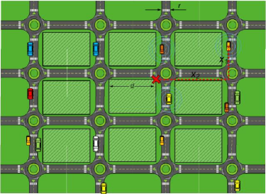
Figure 1: System illustration.

The uplink transmit power level is denoted by $P_{t}$ and the fading channel $h$ for vehicular transmissions is assumed to be Rayleigh with mean equal to unity, $E\{h\}\!=\!1$. The distance-based pathloss in Manhattan grid, $l(x_{1},x_{2})$, is a function of the NLOS distance, $x_{1}$, as well as of the LOS distance $x_{2}$, see also Fig. 1. For a vehicle located at coordinates $(x_{1},x_{2})$, the distance-based pathloss to the origin can be read as $l(x_{1},x_{2})=Cx_{1}^{-2}x_{2}^{-\alpha}$ where the attenuation exponent $\alpha$ along the LOS is taken equal to $2$ and typical values for the NLOS are $4\sim 6$. One may notice that for the $k$-th vertical street $x_{2,k}=kD,k>0$ while for the vertical street facing the considered femto-cell, $k=0$, we have $x_{2,k}=1$. Also, the parameter $C$ accounts for antenna gain, car isolation (in the case of in-car base station) and wall losses with typical wall attenuation in the range of $15\sim 20$ dB.

We want to identify whether uplink vehicular communication and indoor femto-cells can coexist in the same spectrum. In order to do that we evaluate the outage probability for given SIR target $\gamma$ at the worst-case located femto-cell facing a cross-road, see Fig. 1. In order to evaluate the SIR distribution we need a model for the aggregate interference distribution and a model for the wanted signal power level at the femto-cell. Assuming Nakagami-m fading for indoor propagation, the wanted signal power is Gamma distributed with shape $m$ and scale ${\overline{P}}_{rx}/m$ where ${\overline{P}}_{rx}$ denotes the mean received signal power. Next, we propose a model for the interference distribution and evaluate its moments.

3 Modeling interference distribution

The interference level can be expressed as the sum of interference levels from all active car base stations on all vertical and horizontal streets.

$$I_{\Phi} {=} \sum_{k}I_{\Phi_{k}}+\sum_{k^{\prime}}I_{\Phi_{k^{\prime}}}$$

$${=} \sum_{k}\!\!\sum_{x_{i}\in\Phi_{k}}\!\!\!\!P_{t}h_{i}l(x_{1,i},x_{2,k})\!+\!\sum_{k^{\prime}}\!\!\sum_{x_{i^{\prime}}\in\Phi_{k^{\prime}}}\!\!\!\!P_{t}h_{i^{\prime}}l(x_{1,i^{\prime}},x_{2,{k^{\prime}}})$$

where $x_{1,i}$ and $x_{2,k}$ are vertical NLOS distance and horizontal LOS distance, respectively, between $i$-th car on $k$-th vertical street to the crossing toward the victim building, and $x_{1,i^{\prime}}$ and $x_{2,{k^{\prime}}}$ are horizontal NLOS distance and vertical LOS distance, respectively, between ${i^{\prime}}$-th car on ${k^{\prime}}$-th horizontal street to the crossing toward the victim building.

Based on the assumption that vertical/horizontal streets in Manhattan two-dimensional grid are symmetric and a constant car density is used on all the streets, we have same density for the processes $\Phi_{k},\Phi_{k^{\prime}}\forall k,k^{\prime}$, or, $\lambda_{k}\!=\!\lambda_{k^{\prime}}\!=\!\lambda\,\forall k,k^{\prime}$. Also, the independent property of PPP allows us to focus only on one type of street (hereafter, vertical streets) and incorporate the impact of horizontal streets using a scaling factor equal to two. Next, we characterize the distribution of aggregate interference from uplink transmissions located on the $k$-th vertical street, $I_{\Phi_{k}}$, in terms of its LT.

Lemma 1

For Rayleigh fading channels, i.e. $h_{i}\sim\exp(1)$, the LT of the aggregate interference from car base stations distributed as one-dimensional PPP on the $k$-th vertical street in a Manhattan grid is

$$\mathcal{L}_{I_{\Phi_{k}(z)}}(s) {=} \mbox{exp}\left[-\pi\lambda\sqrt{\frac{sz}{\beta_{k}}}\right]$$ (1)

where $z=P_{t}C$ and $\beta_{k}\!=\!x_{2,k}^{\alpha}$. The proof is given in Appendix.

Proposition 2

The total interference from all vertical streets in a Manhattan grid is

$$\mathcal{L}_{I_{\Phi(z)}}(s) {=} \mbox{exp}\left[-\pi\lambda\left\{1+{\zeta\left(\frac{\alpha}{2}\right)}{}D^{-\frac{\alpha}{2}}\right\}\sqrt{sz}\right]$$ (2)

where $\zeta(\cdot)$ denotes the Riemann zeta function. The proof is given in Appendix.

Note that the integral range (refer to the Proof) used in Eq.(1) is from $0$ to infinity, i.e. singular pathloss model. This range causes inaccurate interference modeling in the near-field, since the interference level can become infinite when $x_{1}$ and $x_{2,k}$ become zero. In a more practical case, non-singular path loss model is taken into account by limiting $x_{1}\geq 1$, and apply the integral $\int_{1}^{\infty}(\cdot)dx_{1}$. The results given in Eq. (1) and Eq. (2) can be regenerated through the following Lemma and Proposition.

Lemma 3

For the non-singular path loss model, the interference from the $k$-th vertical street in a Manhattan street is

$$\mathcal{L}_{I_{\Phi_{k}(z)}}(s) {=} \mbox{exp}\left[-2\lambda\sqrt{\frac{sz}{\beta_{k}}}\arctan\left(\sqrt{\frac{sz}{\beta_{k}}}\right)\right].$$

The proof is given in Appendix.

Proposition 4

For the non-singular path loss model, the total interference from all vertical streets in a Manhattan grid is

$$\mathcal{L}_{I_{\Phi(z)}}(s) {=} \mbox{exp}\left[-2\lambda\sum_{k=0}^{\infty}\sqrt{\frac{sz}{\beta_{k}}}\arctan\left(\sqrt{\frac{sz}{\beta_{k}}}\right)\right].$$ (3)

The integral for the inverse LT in Eq. (3) does not exist in closed-form. As a means to provide simple and useful expressions, the use of approximations for the aggregate interference is motivated. Since the LT of the interference with the singular pathloss model in Eq. (2) resembles the Characteristic function of the Levy distribution, we approximate the interference by a fitted inverse Gamma distribution.

The first two moments of the interference can be found based on the LT $\mathbf{E}(I_{\Phi}^{i})=(-1)^{i}\frac{d^{i}}{ds^{i}}\mathcal{L}_{I_{\Phi}}(s)|_{s=0}$ and expressed as following property of the

$$\mathbf{E}\{I_{\Phi}\}\! {=} \!2\lambda\!\sum_{k=0}^{\infty}{\frac{z}{\beta_{k}}}{=}2\lambda z\left(1+\frac{\zeta(\alpha)}{D^{\alpha}}\right)$$

$$\mathbf{E}\{I_{\Phi}^{2}\}\! {=} \!\frac{4\lambda}{3}\!\sum_{k=0}^{\infty}\!{\frac{z^{2}}{\beta_{k}^{2}}}\!+\!\mathbf{E}\{I_{\Phi}\}^{2}{=}\frac{4\lambda z^{2}}{3}\!\!\left(\!1\!+\!\frac{\zeta(2\alpha)}{D^{2\alpha}}\!\right)\!+\!\mathbf{E}\{I_{\Phi}\}^{2}.$$

The fitted inverse Gamma distribution has scale $a=\frac{\mathbf{E}\{I_{\Phi}\}^{2}}{\mathbf{E}\{I_{\Phi}^{2}\}-\mathbf{E}\{I_{\Phi}\}^{2}}+2$ and shape $b={\mathbf{E}\{I_{\Phi}\}}{(a-1)}$. The inverse of the interference distribution is a Gamma distributed random variable with scale $a$ and shape $1/b$, $I_{\Phi}^{-1}\sim{\text{Gamma}}(a,1/b)$.

4 Modeling SIR distribution

For the performance evaluation of wireless systems, assessing the quantity of the signal to interference plus noise ratio (SINR) is required. Based on our system model assumptions, the performance at the worst case femto-cell is limited by the interference level and the impact of noise power can be ignored. The SIR level is

$${SIR}=\frac{P_{rx}}{I_{\Phi}}$$

where $P_{rx}$ is the wanted received signal level.

For ensuring satisfactory services to users of the femto-cell network, the outage probability (i.e. probability that the SIR value is below a target SIR) must be maintained under specific value. The outage probability can be computed using the following Lemma.

Lemma 5

The outage probability when the source destination fading is Nakagami-m distributed, with mean signal level ${\overline{P}}_{rx}$ is

$$\mathbf{P}({SIR}\leq\gamma) = 1-\sum_{i=0}^{m-1}\frac{(-\xi)^{i}}{i!}\frac{d^{i}}{d\xi^{i}}\mathcal{L}_{I_{\Phi(z)}}(\xi)$$ (4)

where $\xi=\frac{m\gamma}{\overline{P}_{rx}}$. The proof is given in the Appendix.

Eq. (4) indicates that the LT of the aggregate interference generated by the car base stations plays a central role in quantifying the outage probability in the femto-cell network. While the outage probability is completely characterized by the LT of the interference, it is also useful to approximate the SIR distribution by some known function so as to assess its mean and higher moments in a low-complex manner.

Note that the useful signal level at the femto-user in the Nakagami-m fading channel is Gamma distributed with scale $m$ and shape $\theta=\frac{\overline{P}_{rx}}{m}$, $P_{rx}\sim$ Gamma($m,\theta$). Hence, with $I_{\Phi}^{-1}\sim{\text{Gamma}}(a,1/b)$ presented in Section 3, the SIR, $P_{rx}\cdot I_{\Phi}^{-1}$, can be expressed as product of two independent Gamma random variables. By normalizing respective shape parameters, the normalized SIR $\gamma_{n}=\frac{b}{\theta}\cdot\frac{P_{rx}}{I_{\Phi}}$ becomes the product of two Gamma random variables with shape equal to unity, $g_{1}=P_{rx}\theta^{-1}\sim$ Gamma($m,1$) and $g_{2}=I_{\Phi}^{-1}{b}\sim$ Gamma($a,1$) and $\gamma_{n}=g_{1}\cdot g_{2}$. In that case the PDF of the normalized SIR distribution can be expressed in terms of the Meijer G functionSpringer

$$\mathbf{P}\left(\gamma_{n}\right) = \frac{G\begin{smallmatrix}2&0\\ 0&2\end{smallmatrix}\left(\begin{smallmatrix}-\\ m,a\end{smallmatrix}\middle|\gamma_{n}\right)}{\Gamma(m)\Gamma(a)}=\frac{2{\gamma_{n}}^{\frac{a+m}{2}}\cdot K_{m-a}(2\sqrt{\gamma_{n}})}{\Gamma(m)\Gamma(a)}$$

where $\Gamma(\cdot)$ is the gamma function, $G(\cdot)$ is Meijer G-function and $K_{m-a}(\cdot)$ is the modified Bessel function of the second kind with order ($m-a$).

The CDF of the normalized SIR distribution is derived using integral properties Springer of the Meijer G-function,

$$\mathbf{P}\left(\frac{b}{\theta}\cdot\frac{S}{I_{\Phi}}\leq\gamma_{n}\right) = \frac{G\begin{smallmatrix}2&1\\ 1&3\end{smallmatrix}\left(\begin{smallmatrix}1\\ m,a,0\end{smallmatrix}\middle|\gamma_{n}\right)}{\Gamma(m)\Gamma(a)}$$ (5)

where $G\begin{smallmatrix}2&1\\ 1&3\end{smallmatrix}\left(\begin{smallmatrix}1\\ m,a,0\end{smallmatrix}\middle|\gamma_{n}\right)=\frac{\Gamma(a-m)\gamma_{n}^{m}}{m}{}_{1}F_{2}(m;m+1-a,m+1;\gamma_{n})+\frac{\Gamma(m-a)\gamma_{n}^{a}}{a}{}_{1}F_{2}(a;a+1-m,a+1;\gamma_{n})$ and ${}_{p}F_{q}(\cdot)$ is the generalized hypergeometric function for integer $p$ and $q$.

Eq. (5) can be used as the CDF of the SIR distribution by properly shifting the axis $\mathbf{P}\left(\frac{b}{\theta}\cdot\frac{S}{I_{\Phi}}\leq\gamma_{n}\right)=\mathbf{P}\left(\frac{S}{I_{\Phi}}\leq\frac{\theta}{b}\gamma_{n}\right)=\mathbf{P}\left(\frac{S}{I_{\Phi}}\leq\gamma\right)$.

5 Numericals

In order to verify the suitability of interference and SIR models presented in Section 3 and Section 4 we consider cars deployed in a city centre which is modeled as a square with side equal to $2$ km. Street width is taken equal to $r\!=\!20$ m and building block is a square with side $d\!=\!50$ m. For NLOS propagation the pathloss exponent is taken equal to $\alpha\!=\!4$. The transmit power level in the uplink is $P_{t}=100$ mW, the wall attenuation is $15$ dB, the attenuation constant is $10^{-3}$. For mounted roof-top antenna, car isolation is equal to $\eta=0$ dB and for in-car base station $\eta=\{10,20,30\}$ dB are considered. For indoor propagation we present results for Rayleigh fading, $m=1$. The mean wanted signal level at the femto-cell is taken equal to $\overline{P}_{rx}=-40$ dBm. In order to evaluate the outage probability at the femto-cell we assume a SIR target equal to $\gamma=15$ dB.

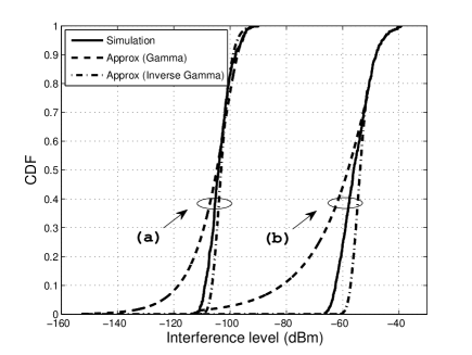
Figure 2: Approximations of interference level distribution using Gamma and Inverse-Gamma distribution with non-singular path-loss model, when (a) the interference from the closest street $k=0$ is not considered and (b) the interference from all vertical streets is considered.

Firstly, we check the accuracy of fitted inverse Gamma distribution for approximating the aggregate interference. For the parameter settings presented above the scale and the shape of the fitted distribution are $a=2.3$ and $b=8.2\cdot 10^{-9}$ respectively. Recall that the inverse Gamma approximation was selected on the basis of the LT of the interference for singular pathloss model in Eq. (2) which resembles the characteristic function of the Levy distribution. For comparison purposes we illustrate the accuracy for a fitted Gamma distribution too, see Fig. 2. Both distributions are accurate in the upper tail which would determine the accuracy of the approximation in the lower tail of the SIR distribution. However, the inverse Gamma distribution achieves better approximation over the full distribution body. In Fig. 2, it is interesting to note that the mean interference level decreases by approximately $50$ dB if the impact of the street facing the femto-cell of interest, $k=0$, is not considered.

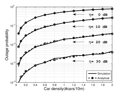
Figure 3: Comparison of outage probability for simulation result and analytical result in Eq. (4) with respect to car base station density $\lambda$ and car isolation $\eta$ when Nakagami fading parameter $m=1$, mean wanted signal level is $\overline{P}_{rx}=-40$ dBm and SIR target is $\gamma=15$ dB.

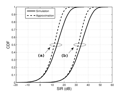
Figure 4: SIR distribution when car base station density is $\lambda=0.1$ Cars/m, the mean wanted signal level is $\overline{P}_{rx}=-40$ dBm, Car isolations are (a) $\eta=0$ dB and (b) $\eta=20$ dB

Secondly, we utilize Eq. (4) for approximating the outage probability at the femto-cell as a function of the density $\lambda$ of uplink transmissions, see Fig. 3. With car isolation equal to $20$ dB or higher, the outage probability decreases at acceptable values even for a high density of vehicles.

The outage probability has been approximated by evaluating the LT of the interference distribution and also its derivatives at certain point, see Eq. (4). The amount of computations might be high particularly when the shape $m$ of the Nakagami distribution is high. The CDF of the SIR distribution has been approximated in Section 4 using the Meijer G function. The approximating CDF can be useful for estimating not only the outage probability but also the moments of the SIR distribution. In Fig. 4 one can observe that the Meijer G function is accurate in the lower tail. However, the mean SIR is underestimated by $2.5$ dB.

6 Conclusion

In dense urban cities vehicular communication may use same spectrum with indoor femto-cells. As a result, better quality of experience for the end-users while on board would most probably come at the cost of higher interference generated indoors. We developed a model that is useful for assessing the outage probability at the femto-cell due to the interference generated from car base stations. With mounted antennas on the top of the vehicles the outage probability becomes prohibitively high given that the density of vehicular transmissions is high too. On the other hand, with in-car base stations, the isolation due to the car shell and the possibility to use lower power levels inside the car make it possible to maintain a low outage probability at the femto-cell even for a high car density. However, in that case, additional spectrum resources are needed as only in-car communication uses same spectrum with indoor femto-cells while street micro-cells are allocated at different spectrum.

APPENDIX

Appendix A Proof of Lemma 1

The distribution of the random variable $I_{\Phi_{k}}$ is characterized in terms of its LT which is given by

$$\mathcal{L}_{I_{\Phi_{k}(z)}}(s) = \mathbb{E}\left[{e}^{-s\cdot I_{\Phi_{k}}}\right]=\mathbb{E}\left[{e}^{-s\cdot\sum_{x_{i}\in\Phi_{k}}P_{t}h_{x_{i}}l(x_{i},x_{2,k})}\right]$$

$$\overset{(p1)}{=} \mathbb{E}_{\Phi_{k}}\left[\prod_{x_{i}\in\Phi_{k}}\mathbb{E}_{h}[{e}^{-s\cdot P_{t}hl(x_{i},x_{2,k})}]\right]$$

$$\overset{(p2)}{=} {e}^{-\lambda\int_{\mbox{${\mathbb{R}}$}}\left(1-\mathbb{E}_{h}\left[{e}^{-s\cdot P_{t}hl(x,x_{2,k})}\right]\right)\mbox{d}x}$$

$$\overset{(p3)}{=} {e}^{-2\lambda\int_{0}^{\infty}\left(1-{\mathbb{E}_{h}\left[{e}^{-s\cdot P_{t}hl(x,x_{2,k})}\right]}\right)\mbox{d}x}$$

$$\overset{(p4)}{=} {e}^{-2\lambda\int_{0}^{\infty}\frac{s\cdot P_{t}l(x,x_{2,k})}{1+s\cdot P_{t}l(x,x_{2,k})}\mbox{d}x}$$

$$\overset{(p5)}{=} {e}^{-2\lambda\int_{0}^{\infty}\frac{sz}{\beta_{k}x^{2}+sz}dx}\overset{(p6)}{=}{e}^{-\pi\lambda\sqrt{\frac{sz}{\beta_{k}}}}$$

where ($p1$) follows from the i.i.d. distribution of the fading $h$, ($p2$) follows from the generating functional Haenggi_large of the one-dimensional PPP, ($p3$) follows from the symmetry of the interference around the origin, and ($p4$) follows from the fact that the fading $h$ follows an exponential distribution with mean equal to unity. ($p5$) follows the pathloss model $l(x,x_{2})=Cx^{-2}x_{2}^{-\alpha}$ and ($p6$) follows from the integration rule $\int_{0}^{\infty}\frac{s}{ux^{2}+s}\mbox{d}x=\frac{\pi}{2}\sqrt{\frac{s}{u}}$ (Zwillinger, , 2.172).

Appendix B Proof of Proposition 2

Since the PPP:s along different vertical streets are independent among each other, the LT of the aggregate interference from all vertical streets is equal to the product of the LT:s from each vertical street

$$\mathcal{L}_{I_{\Phi(z)}}(s) {=} \prod_{k}\mathcal{L}_{I_{\Phi_{k}(z)}}(s){=}{e}^{-\pi\lambda\sum_{k=0}^{\infty}\sqrt{\frac{sz}{\beta_{k}}}}$$ (6)

$$\overset{(p1)}{=} {e}^{-\pi\lambda\left(1+{\zeta\left(\frac{\alpha}{2}\right)}{}D^{-\frac{\alpha}{2}}\right)\sqrt{sz}}$$

where ($p1$) follows from the Riemann zeta function, $\zeta(s)=\sum_{k=1}^{\infty}k^{-s}$ (Zwillinger, , 0.233).

Appendix C Proof of Lemma 3

For the non-singular pathloss model, the interference from $k$-th vertical street is derived by following similar steps to Lemma 2. Only the lower integration limit is different.

$$\mathcal{L}_{I_{\Phi_{k}(z)}}(s) {=} {e}^{-2\lambda\int_{1}^{\infty}\frac{s\cdot Pl(x,x_{2,k})}{1+s\cdot Pl(x,x_{2,k})}dx}={e}^{-2\lambda\int_{1}^{\infty}\frac{sz}{\beta_{k}x^{2}+sz}dx}$$

$$\overset{}{=} {e}^{-2\lambda\int_{1}^{\infty}\frac{1}{(\frac{\beta_{k}}{sz})x^{2}+1}dx}\overset{(p1)}{=}{e}^{-2\lambda\sqrt{\frac{sz}{\beta_{k}}}\arctan\left(\sqrt{\frac{sz}{\beta_{k}}}\right)}$$

where ($p1$) follows from the integration rule $\int_{1}^{\infty}\frac{s}{ux^{2}+s}\mbox{d}x=\sqrt{\frac{s}{u}}\cdot\mbox{arctan}\left(\sqrt{\frac{s}{u}}\right)$ (Zwillinger, , 2.172).

Appendix D Proof of Lemma 5

$$\mathbf{P}(\mbox{SIR}\geq\gamma) = \mathbf{P}\left({h\overline{P}_{rx}}/{I_{\Phi}}\geq\gamma\right)=\mathbf{P}\left(h\geq{\gamma I_{\Phi}}/{\overline{P}_{rx}}\right)$$

$$\overset{(p1)}{=} \int_{0}^{\infty}\mathbf{P}\left(h\geq{\gamma t}/{\overline{P}_{rx}}\right)f_{I_{\Phi}}(t)\mbox{d}t$$

$$\overset{(p2)}{=} \int_{0}^{\infty}\sum_{i=0}^{m-1}\frac{(mxt)^{i}}{i!}e^{-mxt}f_{I_{\Phi}}(t)\mbox{d}t$$

$$\overset{(p3)}{=} \sum_{i=0}^{m-1}\frac{(-mx)^{i}}{i!}\frac{d^{i}}{d(mx)^{i}}\int_{0}^{\infty}e^{-mxt}f_{I_{\Phi}}(x)\mbox{d}x$$

$$= \sum_{i=0}^{m-1}\frac{(-\xi)^{i}}{i!}\frac{d^{i}}{d\xi^{i}}{\mathcal{L}}_{I_{\Phi}}(\xi)$$

where $x=\frac{\gamma}{\overline{P}_{rx}}$ and $\xi=mx$. Equality ($p1$) follows from denoting $f_{I_{\Phi}}(t)$ the PDF of the interference distribution, ($p2$) is based on the fact that when the source-destination fading is Nakagami-m distributed, then the CCDF of $h$ is $\mathbf{P}(h>x)=\sum_{i=0}^{m-1}\frac{(mx)^{i}}{i!}e^{-mx}$, and ($p3$) holds true according to the following Laplace transform property $\int_{0}^{\infty}e^{-st}t^{i}f_{I_{\Phi}}(t)\mbox{d}t=(-1)^{i}\frac{d^{i}}{ds^{i}}{\mathcal{L}}\{f_{I_{\Phi}}\}(s)$.

References

- (1) R. Schneiderman, “Car Makers See Opportunities in Infotainment, Driver-Assistance Systems,” in IEEE Signal Processing Magazine, vol.30, no.1, pp.11-15, 2013.
- (2) J. Gozalvez, M. Sepulcre, and R. Bauza, “IEEE 802.11 p vehicle to infrastructure communications in urban environments,” in IEEE Communications Magazine, vol.50, no.5, pp.176-183, 2012.
- (3) A.U. Sheikh, Wireless communications: theory and techniques. Springer, 2004.
- (4) Y. Sui, J. Vihriälä, A. Papagogiannis, M. Sternad, W. Yang, and T. Svensson, “Moving Cells: A Promising Solution to Boost Performance for Vehicular Users,” in IEEE Communications Magazine, vol.51, no.6, pp.62-68, 2013.
- (5) H. Harri and A.Toskala, LTE Advanced: 3GPP Solution for IMT-Advanced. Wiley.com, 2012.
- (6) B. Kaufman, J. Lilleberg, and B. Aazhang, “Femtocell architectures with spectrum sharing for cellular radio networks” in International Journal of Advances in Engineering Sciences and Applied Mathematics, vol.5, no.1, pp.66-75, 2013.
- (7) M. Haenggi and R. K. Ganti, “Interference in large wireless networks”, in Foundations and Trends in Networking, vol.3, no.2, pp.127-248, 2009.
- (8) P. Cardieri, “Modeling Interference in Wireless Ad hoc Networks,” in IEEE Communications Surveys & Tutorials, vol.12, no.4, pp.551-572, 2010.
- (9) B. Cho, K. Koufos, and R. Jäntti, “Interference control in cognitive wireless networks by tuning the carrier sensing threshold,” in proc. IEEE CrownCom’13, 2013.
- (10) B. Cho, K. Koufos, and R. Jäntti, “Bounding the Mean Interference in Matérn type II Hard-Core Wireless Networks,” in IEEE Wireless Communications Letters, vol.PP, no.99, pp.1-4, 2013.
- (11) K. Ruttik, K. Koufos, and R. Jäntti, “Computation of aggregate interference from multiple secondary transmitters,” in IEEE Communications Letters, vol.15, no.4, pp.437-439, 2011.
- (12) J. G. Andrews, F. Baccelli, and R.K. Ganti, “A tractable approach to coverage and rate in cellular networks. Communications”, in IEEE Transactions on Communications, vol.59, no.11, pp.3122-3134, 2011.
- (13) J.B. Andersen, T. S. Rappaport, and S. Yoshida, “Propagation measurements and models for wireless communications channels,” in IEEE Communications Magazine, vol.33, no.1, pp.42-49, 1995.
- (14) M. D. Springer and W. E. Thompson, “The distribution of products of Beta, Gamma and Gaussian random variables”, in SIAM Journal on Applied Mathematics, vol.18, no.4, pp.721-737, 1970.
- (15) D. Zwillinger and A. Jeffrey, Table of Integrals, Series, and Products, Oxford, UK: Elsevier, 2004.