The impact of spin temperature fluctuations on the 21-cm moments

Abstract

This paper considers the impact of Lyman-$\alpha$ coupling and X-ray heating on the 21-cm brightness-temperature one-point statistics (as predicted by semi-numerical simulations). The X-ray production efficiency is varied over four orders of magnitude and the hardness of the X-ray spectrum is varied from that predicted for high-mass X-ray binaries, to the softer spectrum expected from the hot inter-stellar medium. We find peaks in the redshift evolution of both the variance and skewness associated with the efficiency of X-ray production. The amplitude of the variance is also sensitive to the hardness of the X-ray SED. We find that the relative timing of the coupling and heating phases can be inferred from the redshift extent of a plateau that connects a peak in the variance’s evolution associated with Lyman-$\alpha$ coupling to the heating peak. Importantly, we find that late X-ray heating would seriously hamper our ability to constrain reionization with the variance. Late X-ray heating also qualitatively alters the evolution of the skewness, providing a clean way to constrain such models. If foregrounds can be removed, we find that LOFAR, MWA and PAPER could constrain reionization and late X-ray heating models with the variance. We find that HERA and SKA (phase 1) will be able to constrain both reionization and heating by measuring the variance using foreground-avoidance techniques. If foregrounds can be removed they will also be able to constrain the nature of Lyman-$\alpha$ coupling.

1 Introduction

The cosmic dark ages, during which the only source of radiation was the adiabatically cooling cosmic microwave background (CMB), ended when the first stars formed (see Loeb & Furlanetto 2013 for an overview of this process). The exact nature of the first stars and galaxies is uncertain, but the radiation they emitted will have dramatically altered the state of the intergalactic medium (IGM). Neutral hydrogen (H i) dominates the composition of the IGM until the epoch of reionization (EoR); as such it is hoped that the impact of these galaxies will be detectable with the 21-cm line, a spectral line produced by a hyperfine transition in H i (Field, 1958, 1959). The spin temperature ($T_{\rm s}$), defines the distribution of the electron population over the singlet and triplet hyperfine levels involved in the 21-cm transition (Ewen & Purcell, 1951). If this is in equilibrium with the temperature of the CMB ($T_{\textsc{cmb}}$) then the 21-cm signal will not be detectable. However, radiation from stars breaks this equilibrium, leading to an observable signal in absorption where $T_{\rm s}<T_{\textsc{cmb}}$, and in emission when $T_{\rm s}>T_{\textsc{cmb}}$.

1.1 The impact of the first stars

As well as affecting the spin temperature, radiation from the first stars began ionizing neutral hydrogen. Most important to this discussion is the production of Lyman-$\alpha$, X-ray and ultra-violet radiation.

1. Wouthuysen-Field (Lyman-$\alpha$) coupling:. The populations of the 21-cm hyperfine levels are mixed by repeated absorption and re-emission of Lyman-$\alpha$ radiation. This couples the spin temperature to the Lyman-$\alpha$ colour temperature $T_{\alpha}$. Repeated scattering of Lyman-$\alpha$ photons off atoms couples $T_{\alpha}$ to the kinetic gas temperature ($T_{\rm k}$) and so $T_{\rm s}\sim T_{\rm k}$ (Wouthuysen, 1952; Field, 1958; Pritchard & Furlanetto, 2006). WF coupling therefore produces fluctuations in the 21-cm signal, the observation of which would provide insight into the nature of Lyman-$\alpha$ sources.

2. X-ray heating: An abundance of X-rays are produced by accretion onto compact objects, such as black holes and neutron stars, as well as by hot gas in the interstellar medium. These X-rays induce photo-ionizations resulting in primary and secondary electrons. It is unlikely that X-ray photo-ionizations are efficient enough to be solely responsible for the reionization of the universe (Dijkstra et al., 2004; Hickox & Markevitch, 2007; McQuinn, 2012); however, once the IGM has been ionized to a few percent, the photo-ejected electrons deposit the majority ($\sim 65$%) of their energy as heat in the IGM (Shull, 1979; Shull & van Steenberg, 1985; Furlanetto & Johnson Stoever, 2010). Because the Wouthuysen-Field (WF) coupling described in (i) is likely to have started at an early stage, the onset of X-ray production will raise the 21-cm spin temperature. Observation of 21-cm fluctuations produced by the heating process will therefore provide insight into the nature of X-ray sources.

3. Reionization: As the Universe evolves, Ultra-Violet (UV) radiation from a growing number of galaxies begins to ionize the IGM. These ionizing photons have a short mean-free path and so carve out well defined ionized regions around galaxies in an otherwise mostly neutral IGM. These grow with time until they eventually merge and the Universe is reionized. The associated depletion of neutral gas (and thus 21-cm signal) produces 21-cm fluctuations whose observation will provide insight into the process of reionization (i.e. the nature of the sources responsible, and of the IGM) Whilst sub-dominant to UV ionizations, X-ray induced ionizations will also impact on the ionization state of the IGM (for example, Oh 2001; Venkatesan et al. 2001 and Mesinger et al. 2013).

The exact timing of processes (i)-(iii), and the degree to which they overlap, are uncertain, especially for the coupling and heating processes. This uncertainty depends on the nature of the stars that drive WF coupling and the efficiency (and relative timing) of X-ray production (Mesinger et al., 2013). If the X-ray efficiency is low enough, 21-cm fluctuations induced by X-ray heating may well persist into the EoR.

Despite such uncertainties, it is expected that processes (i) - (iii) occurred in the order described. As the main source of X-rays is thought to be accretion onto compact objects, the production of X-rays is likely to be delayed by a few million years relative to the first stars igniting. Lyman-$\alpha$ production is coincident with formation of the first stars, and the emissivity to achieve Lyman-$\alpha$ coupling is much lower than that required of X-rays to substantially heat the IGM. Therefore Lyman-$\alpha$ coupling will at least commence prior to the onset of X-ray heating (Chen et al., 2004). Because the mean free path of UV photons is very small, UV-driven reionization will inevitably be delayed relative to WF coupling and X-ray heating.

1.2 Constraints on X-ray production from post-EoR redshifts

The only constraints we have on the nature of high-redshift X-ray production come from lower-redshift observations. The dominant X-ray sources observed are active galactic nuclei (AGN) and high-mass X-ray binaries (HMXBs). X-ray emission from the hot interstellar medium (ISM) is also found to contribute significantly to the soft X-ray emission of nearby galaxies (e.g. Mineo et al. 2012b).

Observations of the unresolved cosmic X-ray background point towards AGN being the dominant contributor in the local universe (Moretti et al., 2012). However, the AGN number density rapidly decreases at $z>3$ (see Fan et al. 2001 and references therein), although some scope remains in the faint end of the luminosity function for low-mass ‘mini-quasars’ to contribute at higher redshifts (for example, Madau et al. 2004; Volonteri & Gnedin 2009).

HMXBs are expected to be dominant at high redshift because: (1) in the absence of an AGN they dominate X-ray output in low-redshift galaxies (Fabbiano, 2006), and (2) their abundance is proportional to star-formation rate and ‘starburst’ galaxies are seen to increase with redshift (for example, Gilfanov et al. 2004; Mirabel et al. 2011; Mineo et al. 2012a). Theoretical modelling also suggests that a high fraction of the first stars formed in binaries or multiple systems would evolve into HMXBs (Turk et al., 2009; Stacy et al., 2010).

The X-ray spectral energy distribution (SED) and the associated mean free path of X-rays determine the scale of 21-cm fluctuations produced by inhomogeneous heating. The SED can be fit with a power law where the specific luminosity $L_{\mathrm{X}}$ is proportional to the frequency $\nu$ as $L_{\mathrm{X}}\propto\nu^{-\alpha}$ with spectral energy index of $\alpha$. A harder X-ray SED, with $\alpha<1$, produces higher energy X-rays, which have a longer mean free path. Shocks in supernovae and AGN have an energy index $\alpha\sim 1.7$ (Tozzi et al., 2006; McQuinn, 2012), the hot ISM produces an SED described by $\alpha\sim 3$ (Pacucci et al., 2014), and HMXBs have a hard spectra described by $\alpha\sim 0.7$ - $1$ (Rephaeli et al., 1995; Swartz et al., 2004; Mineo et al., 2012a). Even if we knew the appropriate spectral energy index to describe the SED at high redshift, there is the matter of the luminosity’s normalisation. We can normalise the luminosity at high redshifts to match the low redshift observations, however it could be orders of magnitudes apart from what we observe today.

1.3 Observing and understanding the 21-cm signal

Given that the X-ray properties of high redshift sources are so uncertain there is much to be gained from observing these epochs. The first generation of 21-cm radio telescope such as LOFAR, MWA and PAPER aim to constrain reionization statistically and are already starting to set interesting upper limits (see Paciga et al. 2011; Dillon et al. 2013; Ali et al. 2015 and Pober et al. 2015). However, next-generation instruments HERA and SKA will not only dramatically improve constraints on reionization, but also aim to probe the pre-reionization era. Telescopes seeking to measure the global average of the 21-cm signal, such as EDGES and DARE, should also provide valuable (and complementary) constraints on the EoR and pre-reionization epochs (Bowman & Rogers, 2010; Burns et al., 2012).

Observing the 21-cm line will clearly be rewarding, however it will be challenging as the signal is small ($\sim 10$ mK) and foregrounds will be orders of magnitude larger (Shaver et al., 1999; Di Matteo et al., 2002b; Oh & Mack, 2003; Di Matteo et al., 2004a). It is hoped that by exploiting the spectral smoothness of foregrounds they may be removed (e.g. Wang et al. 2006; Liu & Tegmark 2011; Paciga et al. 2011; Petrovic & Oh 2011; Chapman et al. 2012; Cho et al. 2012; Shaw et al. 2014). Alternatively, we could avoid foregrounds by exploiting the existence of a wedge feature in the $k_{\perp}$-$k_{\parallel}$ cylindrically-binned 2D power spectrum to which foregrounds are confined (e.g. Datta et al. 2010; Vedantham et al. 2012; Morales et al. 2012; Thyagarajan et al. 2013; Hazelton et al. 2013; Liu et al. 2014b). It is not yet clear how well foregrounds can be mitigated (see Liu et al. 2014a), so it is vital that we have a strong understanding of the statistics of 21-cm fluctuations, even in light of next-generation instruments. There are also a large number of astrophysical parameters (many of which are degenerate with each other, see for example Greig & Mesinger 2015 and Pober et al. 2015) for which we have no constraints on in the high-redshift Universe. Therefore we must also fully investigate all possibilities for the range of physics we might observe.

1.4 Overview of this work

Much attention has been focussed on measuring the 21-cm power spectrum, which has been shown to be rich with information (for example, Furlanetto et al. 2004a; Zaldarriaga et al. 2004; Mellema et al. 2006; Lidz et al. 2008; Pritchard & Loeb 2008; Santos et al. 2008; Mesinger et al. 2011; Friedrich et al. 2011; Mesinger et al. 2013; Sobacchi & Mesinger 2014; Greig & Mesinger 2015). However, given the challenging nature of these observations it is also worth considering one-point statistics. One-point statistics have been shown to be information rich, are simpler to interpret, and will be differently affected by foregrounds (e.g. Furlanetto et al. 2004b; Wyithe & Morales 2007; Harker et al. 2009; Ichikawa et al. 2010; Watkinson & Pritchard 2014; Watkinson et al. 2015).

The sensitivity of the 21-cm one-point statistics to coupling and heating has not yet been studied in detail. In this paper we investigate the sensitivity of these statistics to the X-ray efficiency and spectral index using semi-numerical simulations. In doing so, we lift the assumption that $T_{\rm s}\gg T_{\textsc{cmb}}$ (which is often made when simulating reionization) to study the impact of different X-ray properties on the 21-cm moments during the EoR.

We note that during the writing of this paper a similar work by Shimabukuro et al. (2014) was submitted to MNRAS. Our work differs in that our simulated boxes are bigger (theirs are 200 Mpc, ours are 600 Mpc). This is of particular importance in studying X-rays because of their long mean free path, which can be up to hundreds of Mpc (see McQuinn 2012). We also include peculiar velocities in our simulations. Our paper includes several additional elements:

• We present detailed analysis of the impact of X-ray processes on reionization. In particular, we show that the evolution of the skewness is altered in the case of late X-ray heating, providing a useful feature for constraining such models.

• The impact of different values for the spectral index is studied, identifying a degeneracy between X-ray efficiency and spectral index (because both alter the amplitude of the 21-cm variance). This degeneracy may be broken through observations of the 21-cm skewness. This provides sensitivity to the X-ray spectral hardness.

• Finally we consider the prospects for constraining X-ray source properties with current and future generations of radio telescope. In particular, we establish that even if foreground removal is not possible, the 21-cm variance can be accurately measured using foreground avoidance techniques.

The paper is structured as follows: In Section 2 we describe our simulations; in Section 3.1 we study the evolution of the variance and skewness during the epochs of WF coupling and X-ray heating; we then look at the impact of X-ray processes on the moments during reionization in Section 3.2; in Section 4 we consider the observational prospects for constraining the nature of WF coupling, X-ray heating, and reionization using the moments; finally in Sections 5 and 6 we discuss caveats of our work and conclude.

2 Simulation overview

We use the latest public release version of 21CMFAST (v1.12) for this work. For details of this simulation we refer the reader to Mesinger & Furlanetto (2007) and Mesinger et al. (2011); however for convenience we will summarise the main points.

The code uses the Zel’dovich Approximation (Zel’dovich, 1970) applied to linear-density fields to generate evolved density ($\delta$) and velocity ($\operatorname{d}\!{v}_{\rm r}/\operatorname{d}\!{r}$) fields. The excursion-set formalism of Furlanetto et al. (2004b) can then be applied to the evolved density fields to generate neutral-fraction ($x_{\textsc{hi}}$) fields to model UV-driven ionizations. The offset of the brightness temperature relative to that of the CMB ($\delta T_{\rm b}$) can then be calculated (assuming $T_{\rm s}\gg T_{\textsc{cmb}}$) according to,

$$\begin{split}\delta T_{\rm b}=&\frac{T_{\rm s}-T_{\textsc{cmb}}}{1+z}(1-e^{-\tau_{\nu_{0}}})\,,\\ \approx&\,27\,\frac{T_{\rm s}-T_{\textsc{cmb}}}{T_{\rm s}}\,x_{\textsc{hi}}(1+\delta)\left[\frac{H(z)/(1+z)}{\operatorname{d}\!{v}_{\rm r}/\operatorname{d}\!{r}}\right]\\ &\times\left(\frac{1+z}{10}\frac{0.15}{\Omega_{\rm m}h^{2}}\right)^{1/2}\left(\frac{\Omega_{\rm b}h^{2}}{0.023}\right)\rm mK\,.\\ \end{split}$$ (1)

The cosmological parameters in this equation are the Hubble parameter $H(z)$, the matter $\Omega_{\rm m}$, and baryon density parameters $\Omega_{\rm b}$ (where $\Omega_{i}=\rho_{i}/\rho_{\rm c}$ and $\rho_{\rm c}$ is the critical density required for flat universe).

Throughout this paper we adopt a standard $\Lambda$CDM cosmology as constrained by Planck, i.e. $\sigma_{8}=0.829$, $h=0.673$, $\Omega_{\rm m}=0.315$, $\Omega_{\Lambda}=0.685$, $\Omega_{\rm b}=0.049$ and $n_{\rm s}=0.96$ (Planck Collaboration et al., 2014). Our simulations produce 3D boxes with side $L=600\,$Mpc and cubic pixels of side $l_{\rm pix}=1\,$Mpc (initial conditions are calculated at double this resolution). All lengths are co-moving unless otherwise stated.

2.1 X-ray heating and ionizations

This paper focuses on the effects of X-ray heating, as such it is essential that the details of spin temperature fluctuations are included. 21CMFAST calculates the spin temperature according to Field (1958); Hirata (2006),

$$\begin{split}T_{\rm s}^{-1}&=\frac{T_{\textsc{cmb}}^{-1}+x_{\alpha}T^{-1}_{\alpha}+x_{\rm c}T^{-1}_{\rm K}}{1+x_{\alpha}+x_{\rm c}}\,,\\ &\approx\frac{T_{\textsc{cmb}}^{-1}+x_{\alpha}T^{-1}_{\alpha}}{1+x_{\alpha}}\,.\\ \end{split}$$ (2)

The WF-coupling coefficient is defined as $x_{\alpha}=1.7\times 10^{11}(1+z)^{-1}S_{\alpha}J_{\alpha}$ pcm^-2s^-2Hz^-1sr^-1, where $S_{\alpha}\sim 1$ is a factor correcting for detailed atomic physics and $T_{\alpha}$ is the Lyman-$\alpha$ colour temperature. The second equality of Equation LABEL:eqn:spinT follows because the collisional coupling coefficient $x_{\rm c}\approx 0$ during the epoch relevant to this work. Both $S_{\alpha}$ and $T_{\alpha}$ are calculated according to Hirata (2006). For the purpose of our analysis, we define an ‘effective’ coupling co-efficient as $x_{\mathrm{eff}}=x_{\alpha}/(1+x_{\alpha})$ assuming $S_{\alpha}=1$.

The Lyman-$\alpha$ flux ($J_{\alpha}$) has two main origins, (1) X-ray excitation (via photo-electrons) of neutral hydrogen and (2) direct stellar emission between the Lyman limit and the Lyman-$\alpha$ line. Lyman-$n$ photons are redshifted into Lyman-$\alpha$ resonance; therefore, $J_{\alpha}$ is calculated by integrating the photon contribution (as produced via mechanisms 1 and 2) over a series of concentric spherical redshift shells surrounding each pixel. For more detail than provided here, we refer the interested reader to the 21CMFAST  literature listed at the beginning of this section as well as Hirata (2006); Pritchard & Furlanetto (2006); and Pritchard & Furlanetto (2007).

Where WF coupling is saturated, $x_{\rm\alpha}\gg T_{\textsc{cmb}}$ and $T_{\rm s}^{-1}\approx T^{-1}_{\alpha}$; in this regime, the kinetic temperature will be tightly coupled to $T_{\alpha}$ due to the repeated scattering of the Lyman-$\alpha$ photons by hydrogen atoms (Field, 1958). The kinetic temperature (outside of H ii regions at position $\bm{x}$ and at redshift $z$) is calculated by tracking the heating history for that position. This can be calculated using the evolution of $T_{\rm k}(\bm{x},z^{\prime})$ which is predicted by,

$$\begin{split}\frac{\operatorname{d}\!{T}_{\rm k}(\bm{x},z^{\prime})}{\operatorname{d}\!{z}^{\prime}}=&\frac{2}{3k_{\rm\textsc{b}}(1+x_{e})}\frac{\operatorname{d}\!{t}}{\operatorname{d}\!{z}^{\prime}}\sum_{p}\epsilon_{p}+\frac{2T_{\rm k}}{3n_{\rm b}}\frac{\operatorname{d}\!{n}_{\rm b}}{\operatorname{d}\!{z}^{\prime}}\\ &-\frac{T_{\rm k}}{1+x_{e}}\frac{\operatorname{d}\!{x}_{e}}{\operatorname{d}\!{z}^{\prime}}\,,\\ \end{split}$$ (3)

where

$$\begin{split}\frac{\operatorname{d}\!{x}_{e}(\bm{x},z^{\prime})}{\operatorname{d}\!{z}^{\prime}}=&\frac{\operatorname{d}\!{t}}{\operatorname{d}\!{z}^{\prime}}\left[\Gamma_{\rm ion}-\alpha_{\rm A}Cx_{e}^{2}n_{\rm b}f_{\rm\textsc{h}}\right]\,.\\ \end{split}$$ (4)

In calculating the kinetic temperature, 21CMFAST must also calculate the local ionized fraction $x_{e}(\bm{x},z^{\prime})$, which depends on the total baryon number density $n_{\rm b}$, the ionization rate per baryon $\Gamma_{\rm ion}$, the case-A recombination co-efficient $\alpha_{\rm A}$, the clumping factor $C=<n_{\rm\textsc{h}}^{2}>/<n_{\rm\textsc{h}}>^{2}$ (where $n_{\rm\textsc{h}}$ describes the hydrogen number density and we set $C=2$), and finally the hydrogen number fraction $f_{\rm\textsc{h}}$. In addition, the kinetic temperature depends on the heating rate ($\epsilon_{p}$) per baryon for process $p$ (for our discussion the dominant process is X-ray heating) and the Boltzmann constant $k_{\rm\textsc{b}}$.

To calculate X-ray heating and ionization rates at redshift $z^{\prime}$ one must integrate over the full range of frequencies for which photons can contribute energy to these processes. Furthermore, to account for redshifted photons, another integral over redshift ($z^{\prime\prime}$) is required. The X-ray luminosity of sources is assumed to be well described by a power law, i.e. $L_{\rm emitted}\propto(\nu/\nu_{0})^{-\alpha}$ (where $\alpha$ is the spectral index discussed in Section 1.2) and $h\nu_{0}$ is the lowest energy X-ray that can escape into the IGM). 21CMFAST assumes that the total X-ray emission rate per second ($\operatorname{d}\!{}\dot{N}/\operatorname{d}\!{z}^{\prime\prime}$) from a spherical shell bounded by the redshift interval $z^{\prime\prime}$ to $z^{\prime\prime}+\operatorname{d}\!{z}^{\prime\prime}$ is the product of the number of X-ray photons per solar mass in stars $\zeta_{\textsc{x}}$ (the X-ray efficiency parameter) and the star formation rate in that shell (SFR${}_{z^{\prime\prime}}$) (i.e. $\operatorname{d}\!{}\dot{N}/\operatorname{d}\!{z}^{\prime\prime}=\zeta_{\textsc{x}}\mathrm{SFR}_{z^{\prime\prime}}$). The arrival rate at position $\bm{x}$ and redshift $z^{\prime}$ from sources between $z^{\prime\prime}$ and $z^{\prime\prime}+\operatorname{d}\!{z}^{\prime\prime}$ is then,

$$\begin{split}\frac{\operatorname{d}\!{\phi}(\bm{x},\nu,z^{\prime},z^{\prime\prime})}{\operatorname{d}\!{z}^{\prime\prime}}=\frac{\operatorname{d}\!{}\dot{N}}{\operatorname{d}\!{z}^{\prime\prime}}\alpha\nu_{0}^{-1}\left(\frac{\nu}{\nu_{0}}\right)^{-\alpha-1}\left(\frac{1+z^{\prime\prime}}{1+z^{\prime}}\right)^{-\alpha-1}\mathrm{e}^{-\tau_{\rm x}}\,,\end{split}$$ (5)

where $\tau_{\rm x}$ is the optical depth of X-rays. In calculating the mean free path of X-rays, fluctuations of the IGM state are ignored. Note that this is very inaccurate during the advanced stages of reionization, when there are large ionized regions in an otherwise neutral IGM. With this approximation, the heating rate due to X-rays at position $\bm{x}$ and redshift $z^{\prime}$ is calculated as,

$$\begin{split}\epsilon_{\rm X}(\bm{x},z^{\prime})=&\int_{\mathrm{Max[\nu_{0},\nu_{\tau=1}]}}^{\infty}\operatorname{d}\!{\nu}\\ &\times\sum_{i}(h\nu-E_{i}^{\rm th})f_{\rm heat}f_{i}x_{i}\sigma_{i}\\ &\times\int_{z^{\prime}}^{\infty}\operatorname{d}\!{z}^{\prime\prime}\frac{\operatorname{d}\!{\phi}/\operatorname{d}\!{z}^{\prime\prime}}{4\pi r_{\rm p}^{2}}\,,\end{split}$$ (6)

where $r_{\rm p}$ is the proper (null geodesic) separation of $z^{\prime}$ and $z^{\prime\prime}$. Under the same assumption, the ionization rate due to X-rays may be described by,

$$\begin{split}\Gamma_{\rm ion}(\bm{x},z)=&\int_{\mathrm{Max[\nu_{0},\nu_{\tau=1}]}}^{\infty}\operatorname{d}\!{\nu}\sum_{i}f_{i}x_{i}\sigma_{i}F_{i}\\ &\times\int_{z^{\prime}}^{\infty}\operatorname{d}\!{z}^{\prime\prime}\frac{\operatorname{d}\!{\phi}/\operatorname{d}\!{z}^{\prime\prime}}{4\pi r_{\rm p}^{2}}\,,\\ \end{split}$$ (7)

$$\begin{split}F_{i}=&(h\nu-E_{i}^{\rm th})\left(\frac{f_{\rm ion,H\textsc{i}}}{E_{\rm H\textsc{i}}^{\rm th}}+\frac{f_{\rm ion,He\textsc{i}}}{E_{\rm He\textsc{i}}^{\rm th}}+\frac{f_{\rm ion,He\textsc{ii}}}{E_{\rm He\textsc{ii}}^{\rm th}}\right)+1\,.\\ \end{split}$$ (8)

In Equations 6 to 8 a sum is taken over the species $i=$H i, He i, He ii; $x_{i}$ is the ionization fraction for the species, $f_{i}$ is the species number fraction, $\sigma_{i}$ is the ionization cross section, and $E_{i}^{\rm th}$ is the species ionization threshold energy. The fraction of the primary electron’s energy that is transferred to heat and secondary ionizations is described by $f_{\rm heat,i}$ and $f_{\rm ion,i}$ respectively for each species. The unity term in $F_{i}$ accounts for primary ionizations of species $i$. The heating and ionization rate are simplified further (to speed up the calculation) by assuming that no photons with an optical depth $\tau\leq 1$ are absorbed by the IGM and all photons with $\tau>1$ are (Mesinger & Furlanetto, 2007; Mesinger et al., 2011).

2.2 UV Ionizations

Ionizations by UV photons are calculated independently from, and following the simulation of X-ray heating and WF coupling. The code smooths iteratively around each pixel in the box from a maximum radius $R_{\rm max}$ down to pixel scales $R_{\rm pix}$. At each smoothing step, on scale $R$, the condition $f_{\rm coll}(\mathbf{x},z,R)\geq\zeta_{\rm uv}^{-1}$ is evaluated, if met the central pixel is marked as ionized; if this condition is never met then the pixel is partially ionized, accounting for both UV ionizations, calculated as $x^{\mathrm{uv}}_{\mathrm{ion}}=\zeta_{\rm uv}f_{\rm coll}(\mn@boldsymbol{r},z,R_{\rm pix})$, and partial ionizations due to X-rays (calculated using Equation LABEL:eqn:xe).

The collapsed fraction $f_{\rm coll}$ is calculated using the prediction of the extended Press-Schechter formalism (Bond et al., 1991; Lacey & Cole, 1993), with the minimum mass corresponding to a virial temperature of 10⁴ K (necessary for cooling by atomic hydrogen to be effective). The collapse fraction is normalised so that its mean agrees with that predicted by the parametrically fit mass function of Jenkins et al. (2001).

The ionizing efficiency of stars is defined as $\zeta_{\rm uv}=f_{\rm esc}f_{*}N_{\gamma/b}(1+n_{\rm rec})^{-1}$, where $f_{\rm esc}$ is the fraction of ionizing photons that escape, $N_{\gamma/b}$ denotes the number of ionizing photons produced per baryon in stars, and finally $n_{\rm rec}$ is the typical number of times that hydrogen will have recombined. The fraction of baryons converted to stars $f_{*}$ also impacts upon the estimation of SFR used in the X-ray heating and ionization rates. We set $\zeta_{\rm uv}=16$ for consistency with our previous publications, and so that the 50% point of reionization falls in the redshift range to which first generation instruments are most sensitive, whilst agreeing with observational constraints on the EoR. Our reionization model is thus optimistic.

Because UV photons have a short mean free path, it is assumed that they will carve out large ionized regions in a mostly neutral IGM; it is useful then to consider the volume filling factor of these ionized H ii regions $Q_{\rm\textsc{hii}}$. The average ionized fraction of the box, taking into account the X-ray ionizations discussed above, is $\overline{x}_{\mathrm{ion}}=Q_{\rm\textsc{hii}}+(1-Q_{\rm\textsc{hii}})x_{e}$.

3 Results

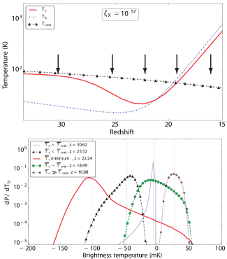
Figure 1: Redshift evolution of the spin ($T_{\rm s}$), kinetic ($T_{\rm k}$), and CMB ($T_{\textsc{cmb}}$) temperatures (top), and brightness-temperature PDF (bottom) at five key phases of its evolution for the fiducial model with $\zeta_{\textsc{x}}=10^{57}$ and $\alpha=1.5$. All PDFs are from maps smoothed to 4 Mpc. Arrows on the top plot correspond to the redshifts for which we present PDFs. The nature and timing of these features are model dependent; in some extreme models it is possible that not all of the five phases we describe will exist, or that their PDFs will look quite different.

In this work, we study the properties of X-ray sources by varying the luminosity normalisation and spectral index. The normalisation of the luminosity is parametrised through the X-ray efficiency parameter $\zeta_{\textsc{x}}$ in 21CMFAST . We simulate $\zeta_{\textsc{x}}=[10^{55},10^{56},10^{57},10^{58}]$, with $\zeta_{\textsc{x}}=10^{57}$ (roughly 1.7 X-ray photons per stellar baryon) as our fiducial model. This choice is consistent with low-redshift constraints on the total X-ray luminosity per unit of star formation (with $f_{*}=0.1$). We then consider the hardness of the X-ray background by varying the spectral index, assuming values ranging from $\alpha=0.8$ (to approximate the spectrum produced by HMXB) to $\alpha=3.0$ (typical of a soft X-ray background as produced by the hot ISM). We set $\alpha=1.5$ in our fiducial model, as it is in the middle of the plausible range of values for this parameter and is representative of X-ray hardness in the local Universe (see the discussion in Section 1.2). Unless otherwise stated results are from maps that have been smoothed and re-sampled to produce pixels with side 4 Mpc. This is to overcome the impact of a discretisation effect (that occurs through the creation of the non-linear density fields) on the moments (see Watkinson & Pritchard 2014 for details).

Ignoring fluctuations in peculiar velocities and at a fixed redshift (and cosmology), the drivers of brightness-temperature fluctuations are the density, neutral-fraction ($x_{\textsc{hi}}=1-x_{\mathrm{ion}}$) and spin-temperature fields; specifically,

$$\begin{split}\delta T_{\rm b}\propto\mu\,x_{\textsc{hi}}\Delta\,,\\ \end{split}$$ (9)

with $\mu=1-T_{\textsc{cmb}}/T_{\rm s}$ and $\Delta=1+\delta$. At early times, before the epoch of reionization, $x_{\textsc{hi}}\sim 1$ and fluctuations in $\mu$ and $\Delta$ dominate the signal. Therefore any evolution of the brightness temperature away from that of the density field will be due to correlations between $\mu$ and $\Delta$. As such we can gain insight by looking at the cross averages of these quantities, which can be broken up as follows,

$$\begin{split}\langle\mu\,x_{\textsc{hi}}\Delta\rangle&=\overline{x}_{\rm H\thinspace\textsc{i}}-\left\langle\delta\frac{T_{\textsc{cmb}}}{T_{\rm s}}x_{\textsc{hi}}\right\rangle-\left\langle\frac{T_{\textsc{cmb}}}{T_{\rm s}}x_{\textsc{hi}}\right\rangle+\left\langle\delta x_{\textsc{hi}}\right\rangle\,;\\ \mathrm{or\,when}\,x_{\textsc{hi}}=1\mathrm{:}\\ \langle\Delta\,\mu\rangle&=1-\left\langle\delta\frac{T_{\textsc{cmb}}}{T_{\rm s}}\right\rangle-\left\langle\frac{T_{\textsc{cmb}}}{T_{\rm s}}\right\rangle\,.\\ \end{split}$$ (10)

3.1 Coupling and heating epochs

\begin{overpic}[trim=0.0pt 8.5359pt 0.0pt 0.0pt,clip={true}]{Images/fig2} \put(83.0,-6.0){-125} \put(128.0,-6.0){-100} \put(175.0,-6.0){-75} \put(219.0,-6.0){-50} \put(264.0,-6.0){-25} \put(313.0,-6.0){0} \put(355.0,-6.0){25} \put(400.0,-6.0){50} \end{overpic}

Figure 2: Brightness-temperature maps of our fiducial ($\zeta_{\textsc{x}}=10^{57}$, $\alpha=1.5$) simulation. Maps are from boxes of side $L=600\,$Mpc smoothed to have pixels of (4 Mpc)³ and presented with the pixel depth flattened into the page. Maps correspond to the five key phases we describe in the text; i.e. $z\sim 30$ where $\overline{T}_{\mathrm{s}}\sim\overline{T}_{\textsc{cmb}}$ (left), $z\sim 25$ where $\overline{T}_{\mathrm{s}}<\overline{T}_{\textsc{cmb}}$ (middle-left), $z\sim 22$ where $\overline{T}_{\mathrm{s}}$ is at its minimum (middle), $z\sim 18$ where $\overline{T}_{\mathrm{s}}\sim\overline{T}_{\textsc{cmb}}$ (middle-right) and $z\sim 16$ where $\overline{T}_{\mathrm{s}}\gg\overline{T}_{\textsc{cmb}}$ (right). The amplitude of the signal is model dependent, the more efficient the X-ray production the less the amplitude in absorption. If the X-ray efficiency is high enough, it is even possible that the signal will never enter a phase of absorption as seen in this fiducial model.

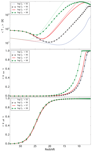
Figure 3: Redshift evolution of: spin (thick lines) and kinetic (thin lines) temperatures (top); ionized fraction (middle); and effective coupling coefficient (bottom). $\alpha=1.5$ for all models. Only in the extremely X-ray-efficient $\zeta_{\textsc{x}}=10^{58}$ model do X-ray ionizations contribute substantially to reionization. All other models exhibit a very similar, UV-driven, reionization history. However, the evolution of the spin temperature is different between all models.

Before considering the evolution of the 21-cm moments, we can build some insight by looking at the probability density function (PDF) of the brightness temperature. The top plot of Fig. 1 shows the redshift evolution of the three temperature components relevant to $\delta T_{\rm b}$: the kinetic temperature ($T_{\rm k}$; blue-dashed line), the CMB temperature ($T_{\textsc{cmb}}$; black-dashed line w/triangles) and the spin temperature ($T_{\rm s}$; red solid line). The bottom plot of the same figure shows the shape of the $\delta T_{\rm b}$ PDF at five important phases of the brightness-temperature’s evolution for our fiducial model (see Shimabukuro et al. 2014 for discussion of the $1-T_{\textsc{cmb}}/T_{\rm s}$ PDF, which agrees with the interpretation we present below).

For reference, the associated brightness-temperature maps are presented in Fig. 2 along with the redshift evolution of spin temperature, ionized fraction and $x_{\mathrm{eff}}$ in Fig. 3 (top, middle and bottom respectively).

• $\bm{\overline{T}_{\rm s}\sim\overline{T}_{\textsc{cmb}}}$, $\bm{z\sim 30}$ (Blue dot-dashed line in Fig. 1 bottom): WF coupling begins almost immediately in our simulations and is positively correlated with the density field (this can be seen in the plot of the cross average of the ‘effective’ WF coupling coefficient with density as a function of redshift in the bottom of Fig. 4). As such the spin temperature in overdense regions (near the sources of Lyman-$\alpha$ radiation) is becoming coupled to the gas temperature (which is cooling adiabatically with the expansion of the universe). As a result the mean spin temperature drops below that of the CMB. This process produces a negatively skewed brightness-temperature PDF which is quite sharply peaked with the weight of the distribution towards more negative brightness temperatures. At this point, brightness-temperature fluctuations are dominated by fluctuations in the density and Lyman-$\alpha$ flux.

• $\bm{\overline{T}_{\rm s}<\overline{T}_{\textsc{cmb}}}$, $\bm{z\sim 25}$ (black dashed line with triangles in Fig. 1 bottom): The Lyman-$\alpha$ coupling coefficient and the density field are most strongly correlated around this epoch for all models presented in this paper (again refer to Fig. 4 bottom). As the Lyman-$\alpha$ coupling becomes more effective the spin temperature starts to evolve more rapidly towards gas temperature, and the skewness of the PDF becomes less negative (as the statistics of the density field become increasingly influential). The variance is increasing during this phase.

• $\bm{\overline{T}_{\rm s}}$ at its minimum, $\bm{z\sim 22}$ (red solid line in Fig. 1 bottom): Eventually the spin temperature reaches a minimum just before coupling fully with the (now increasing) gas temperature. From the PDF we can see that despite the average brightness temperature being at its minimum, some more extreme pixels are already in emission; i.e. coupling and X-ray heating are both very strong in some pixels. At this point, the PDF has a positive skewness, primarily driven by fluctuations in the X-ray heating but amplified by fluctuations in the WF-coupling. This is because a region that is less strongly coupled will have a spin temperature closer to that of the CMB; a region that is both strongly coupled and more heated than the mean will also result in a spin temperature closer to that of the CMB.

• $\bm{\overline{T}_{\rm s}\sim\overline{T}_{\textsc{cmb}}}$ again, $\bm{z\sim 18}$ (Green dashed line w/circles in Fig. 1 bottom): The spin temperature is now fully coupled to the gas temperature and is thus increasing due to X-ray heating. At this point, fluctuations in the X-ray heating are dominating those of the brightness temperature. The average brightness temperature is zero, and fluctuations produce a relatively even distribution of pixels in emission and absorption; therefore the skewness is close to zero. The variance is also decreasing as X-ray heating is becoming more homogeneous.

• $\bm{\overline{T}_{\rm s}\gg\overline{T}_{\textsc{cmb}}}$, $\bm{z\sim 16}$ (Pink dotted line with stars in Fig. 1 bottom): Eventually the spin temperature becomes much greater than the CMB temperature and heating fluctuations become unimportant. This results in a nearly Gaussian distribution as the brightness-temperature fluctuations are governed nearly entirely by those of the density field. Reionization by UV photons is just becoming effective around this time. An earlier reionization model and/or less efficient X-ray production could mean that this Gaussian phase never occurs; instead there may be a phase in which fluctuations in both the heating and ionization fields occur at the same time (as seen in the extreme $\zeta_{\textsc{x}}=10^{55}$, which we describe at length in Section 3.2).

It is important to note that the PDFs described are from our fiducial ($\zeta_{\textsc{x}}=10^{57}$, $\alpha=1.5$) model. Thus, these five points may be observed at different redshifts; the evolution of the PDFs will also vary quantitatively in different models. Furthermore, if X-ray production is either extremely efficient, or extremely inefficient, then the evolution of the various temperatures and therefore the PDFs will be qualitatively different from the fiducial model.

3.1.1 Efficiency of X-ray production

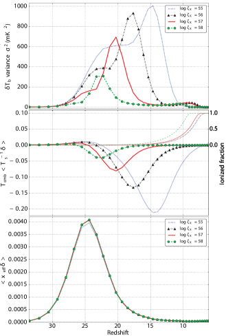
Figure 4: Redshift evolution of: brightness-temperature variance (top) which exhibits two peaks prior to that of reionization; the first is driven by $\langle x_{\mathrm{eff}}\delta\rangle$ (bottom) and the second by $\langle(T_{\textsc{cmb}}/T_{\rm s})\delta\rangle$ (middle). Thin lines on the middle plot correspond to the evolution of the ionized fraction for each model. Statistics are calculated from maps resolved to 4 Mpc, and $\alpha=1.5$ for all models.

Fig. 4 (top) shows the redshift evolution of the brightness-temperature PDF’s variance. The variance is zero at very high redshift for all models. It then increases with decreasing redshift, driven by a slight positive correlation between the density field and $T_{\rm s}^{-1}$; i.e. the spin temperature is smaller in overdense regions, because WF-coupling is strongest in the vicinity of sources and during this phase $T_{\rm k}<T_{\textsc{cmb}}$. This is illustrated by the evolution of $\langle T_{\textsc{cmb}}\delta/T_{\rm s}\rangle$ shown in the middle plot of Fig. 4. The evolution of the variance plateaus briefly as the average spin temperature drops towards the average gas temperature (although note this is less evident in the $\zeta_{\textsc{x}}=10^{58}$ as X-ray heating occurs so early). Eventually an anti-correlation between the density field and $T_{\rm s}^{-1}$ develops. By this point, WF-coupling fluctuations are minimal (see the bottom plot of Fig. 4) and so this effect is caused by the underdense regions being less heated by X-rays than those closer to sources; i.e. the spin temperature is smallest in underdense regions where there are less X-ray sources. In all but the $\zeta_{\textsc{x}}=10^{55}$ model, the variance is largest when this anti-correlation is maximized. As we will see, the $\zeta_{\textsc{x}}=10^{55}$ model enters this phase during the early stages of the EoR, when fluctuations in $x_{\textsc{hi}}$ are becoming influential. However, even in this model the influence of $x_{\textsc{hi}}$ is small, so the amplitude and position of the variance’s maximum should provide a constraint on the X-ray production efficiency. The extent of the plateau that precedes it could provide insight into the relative timing between the onset of WF-coupling and X-ray heating.

We can gain insight into the variance’s strong dependence on the correlation between $T_{\rm s}^{-1}$ and $\delta$ by calculating the variance of $\Delta\mu$. We find that,

$$\begin{split}\sigma^{2}_{\Delta\mu}&=\left\langle\left(\delta\frac{T_{\textsc{cmb}}}{T_{\rm s}}-\delta\right)^{2}\right\rangle+2\left\langle\delta\left(\frac{T_{\textsc{cmb}}}{T_{\rm s}}\right)^{2}\right\rangle\\ &-2\left\langle\delta\frac{T_{\textsc{cmb}}}{T_{\rm s}}\right\rangle-\left\langle\delta\frac{T_{\textsc{cmb}}}{T_{\rm s}}\right\rangle^{2}\\ &-2\left\langle\delta\frac{T_{\textsc{cmb}}}{T_{\rm s}}\right\rangle\left\langle\frac{T_{\textsc{cmb}}}{T_{\rm s}}\right\rangle\,,\\ \end{split}$$ (11)

and see that the variance is only sensitive to $\langle T_{\textsc{cmb}}/T_{\rm s}\rangle$ in the final term where its influence will be suppressed by a factor of $\langle T_{\textsc{cmb}}\delta/T_{\rm s}\rangle$.

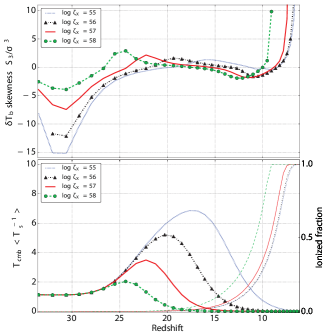
Figure 5: Redshift evolution of the brightness-temperature skewness (top) which exhibits a minimum associated with the onset of WF coupling, followed by a maximum that is driven by $\langle T_{\textsc{cmb}}/T_{\rm s}\rangle$ (bottom). Thin lines on the bottom plot correspond to the evolution of the ionized fraction for each model. Statistics are calculated from maps resolved to 4 Mpc, and $\alpha=1.5$ for all models.

In contrast, we find that the skew of $\Delta\mu$ (for which we include the full equation in Appendix A) is sensitive to both of these terms independently and in combination. The position and amplitude of the maximum in the skewness during this heating phase is mainly sensitive to $\langle T_{\textsc{cmb}}/T_{\rm s}\rangle$ as this factor dominates over $\langle T_{\textsc{cmb}}\delta/T_{\rm s}\rangle$. This is clear from Fig. 5 where we plot the skewness (top) and $\langle T_{\textsc{cmb}}/T_{\rm s}\rangle$ (bottom) as functions of redshift. Initially the skewness becomes increasingly negative during the early stages of WF-coupling. There is a universal minimum to the skewness of our models at $z\sim 31$ driven by fluctuations in the WF-coupling (the details of which are unchanged between models) drawing the spin temperature towards the lower kinetic temperature (see the discussion surrounding Fig. 1). The skewness increases from this minimum, becoming positive and reaching a maximum as the average spin temperature (depicted in the top plot of Fig. 3) reaches its lowest point. At this point, the $\mu$ parameter will be greatest and so fluctuations in the spin temperature dominate.

As previously discussed, we see from the plot of $\langle T_{\textsc{cmb}}/T_{\rm s}\rangle$ in the bottom plot of Fig. 5 that the amplitude of the X-ray heating skewness maximum is inversely proportional to that of $\langle T_{\textsc{cmb}}/T_{\rm s}\rangle$. We find this to be due to contributions from negative $\langle T_{\textsc{cmb}}/T_{\rm s}\rangle^{3}$ terms becoming more dominant as the spin temperature decreases (see Appendix A).

Note that in the $\zeta_{\textsc{x}}\leq 10^{56}$ models, the ionization field is becoming influential as the skewness reaches its global maximum. If we plot the redshift evolution of $\langle T_{\textsc{cmb}}x_{\textsc{hi}}/T_{\rm s}\rangle$ then we find a perfect correlation between the peak in skewness and the minimum of this cross average. Even in such models, the high redshift maximum of the brightness-temperature skewness should provide constraints on the point at which the spin temperature is minimum, and thus the efficiency of X-ray production.

Shimabukuro et al. (2014) show the brightness-temperature variance and skewness for their fiducial model ($\zeta_{\textsc{x}}=10^{56}$). We mostly agree with their findings; however, their plot of the brightness-temperature variance only exhibits the X-ray heating peak (note their plot does not show the redshifts associated with reionization). The peak we associate with WF coupling and the plateau connecting it to the X-ray heating peak is totally absent. This may be because their boxes are small compared with ours. However, it is most likely that this difference is because Shimabukuro et al. (2014) do not smooth their brightness-temperature maps prior to measuring one-point statistics, while we do..

3.1.2 Hardness of the X-ray SED

Fig. 6 (top) shows the redshift evolution of the brightness-temperature variance for different choices of spectral index, with $\zeta_{\textsc{x}}=10^{57}$. The variance for the $\alpha=3.0$ (soft) model is more than double that of the $\alpha=0.8$ (hard) model. The softer the X-ray spectrum the greater the anti-correlation between the density field and $T_{\rm s}^{-1}$ (i.e. the spin temperature is smallest in underdense regions). This is evident in the bottom of Fig. 6 where we plot the redshift evolution of $\langle T_{\textsc{cmb}}\delta/T_{\rm s}\rangle$. This is to be expected as soft X-rays have a shorter mean free path than hard X-rays.

The sensitivity of the variance amplitude to the spectral index is degenerate with changes in amplitude produced by different X-ray efficiencies. This degeneracy maybe broken as the location and amplitude of the skewness’ X-ray heating peak is insensitive to variations of the spectral index (as seen in Fig. 7 in which we plot the skewness for different spectral indices, with $\zeta_{\textsc{x}}=10^{57}$). This is because, the redshift at which the spin temperature minimizes, and the difference between it and $T_{\textsc{cmb}}$, is driven primarily by the efficiency of X-ray production.

We expect the insensitivity of the skewness to the X-ray spectral hardness to be relatively model independent across the models we consider, as $\langle T_{\textsc{cmb}}\delta/T_{\rm s}\rangle\ll\langle T_{\textsc{cmb}}/T_{\rm s}\rangle$ for all (see the bottom of Fig. 4 and Fig. 5). However, should the X-ray production be so efficient that $\langle T_{\textsc{cmb}}/T_{\rm s}\rangle$ remains very small during this phase, then the skewness would be sensitive to $\langle T_{\textsc{cmb}}\delta/T_{\rm s}\rangle$, and therefore the X-ray spectral hardness. We conclude that if the efficiency can be constrained using the skewness, then the amplitude of the variance has potential for constraining the spectral index of the X-ray SED.

Pacucci et al. (2014) find the peak amplitude of the large-scale ($k\sim 0.2\,$Mpc^-1) power spectrum to be sensitive to the X-ray SED’s spectral index, but not the efficiency of X-ray production. We do not recover this behaviour by measuring the variance from maps smoothed on large scales. We find instead that, for smoothing scales of order 60 Mpc, sensitivity to the spectral hardness is lost whilst the amplitude remains sensitive to the efficiency of X-ray production. This suggests that the variance and power spectrum may be complementary in that the large-scale power spectrum can inform us on the spectral index and the variance smoothed on large scales can provide constraints on the efficiency of X-ray production.

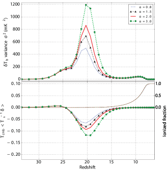
Figure 6: Evolution of variance with redshift (top) for various values of the spectral index of the X-ray SED; $\zeta_{\textsc{x}}=10^{57}$ for all. We find that suppression of the $\langle\delta(T_{\textsc{cmb}}/T_{\rm s})\rangle$ amplitude caused by a harder X-ray spectrum, and seen in the bottom plot (for which the model key of the top plot applies), reduces the variance. Thin lines on the bottom plot correspond to the evolution of the ionized fraction for each model. Statistics are calculated from maps resolved to 4 Mpc.

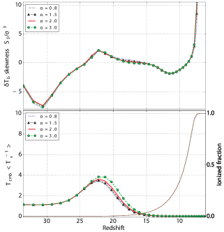
Figure 7: Evolution of the brightness-temperature skewness with redshift (top) for various values of the spectral index of the assumed X-ray SED; $\zeta_{\textsc{x}}=10^{57}$ for all. As $\langle T_{\textsc{cmb}}/T_{\rm s}^{-1}\rangle$ (shown in the bottom plot as a function of redshift) is insensitive to the hardness of the X-ray spectrum, the skewness is not sensitive to the X-ray spectral index. Thin lines on the bottom plot correspond to the evolution of the ionized fraction for each model. Statistics are calculated from maps resolved to 4 Mpc.

3.2 Epoch of reionization

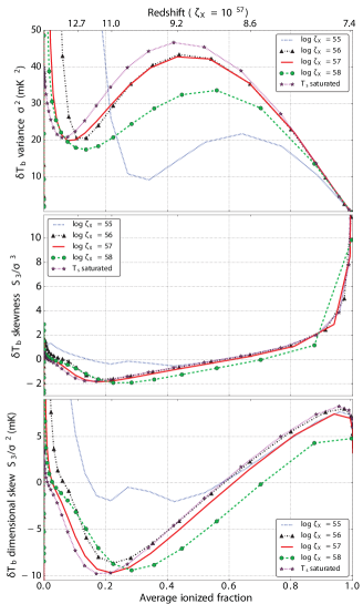
Figure 8: Brightness-temperature variance (top), skewness (middle) and dimensional skewness (bottom) as a function of ionized fraction to highlight features relevant to reionization. X-ray ionizations are seen to reduce the amplitude of the variance (see the green dashed line with circles) by reducing the anti-correlation between density and neutral-fraction fields. If heating is very late (see the blue-dashed line) the turnover in the variance is no longer at the mid-point of reionization, which could lead to misinterpretation of the timing of the EoR. The skewness is qualitatively different in such a model, exhibiting a local maxima during the early stages of reionization (note that the nature of this feature will be extremely model dependent in this regime); such a feature could be used to constrain late X-ray heating models. Statistics are calculated from maps resolved to 4 Mpc, and $\alpha=1.5$ for all models.

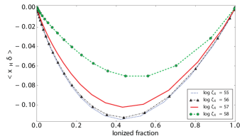
Figure 9: Evolution of the $\langle x_{\textsc{hi}}\delta\rangle$ cross average as a function of ionized fraction; this confirms that it is the decrease in the negativity of $\langle\delta x_{\textsc{hi}}\rangle$ that reduces the variance in the $\zeta_{\textsc{x}}=10^{58}$ model. Statistics are calculated from maps resolved to 4 Mpc, and $\alpha=1.5$ for all models.

When simulating reionization, it is often assumed that the spin temperature is totally saturated and therefore its fluctuations can be ignored. We see in Fig. 8 (in which we plot the brightness-temperature moments as a function of ionized fraction) that this may not be an appropriate assumption. Note that Mesinger et al. (2013) discuss trends in the power spectrum’s evolution at $k=0.1\,$Mpc^-1 similar to those seen in the variance.

3.2.1 The impact of X-ray ionizations during reionization

The variance (Fig. 8 top) for all our models is suppressed relative to that of a simulation that uses identical initial conditions but ignores spin temperature fluctuations (labelled here as ‘$T_{\rm s}$ saturated’). This is due to partial ionization of neutral regions by X-rays. X-ray ionizations are effective in both over and under-dense regions, reducing the anti-correlation between the density and neutral-fraction fields. This is seen in Fig. 9, in which we plot $\langle x_{\textsc{hi}}\delta\rangle$ as a function of ionized fraction, as the anti-correlation reduces with increasing X-ray efficiency. Partial ionizations also shift the mid-point maximum in the variance to higher ionized fractions, as reionization is more advanced when driven just by UV radiation. Such a shift is also seen in the minimum of the skewness and dimensional skewness associated with $\bar{x}_{\rm ion}\sim 0.2$ (see the middle and bottom plots of Fig. 8 respectively).

The late-time features of both skewness statistics at $\bar{x}_{\rm ion}\sim 0.95$, i.e. the rapid increase in the skewness as reionization advances, and a turnover in the dimensional skewness, are far more robust. Although, for the highest efficiency we consider ($\zeta_{\textsc{x}}=10^{58}$) the late-time turnover in the dimensional skewness doesn’t occur, as X-ray ionizations complete reionization early relative to a UV-only model. In the middle plot of Fig. 3, we see that reionization completes at $z\sim 9$ in the $\zeta_{\textsc{x}}=10^{58}$ model; however, models which are mostly driven by UV ionizations don’t reach $\bar{x}_{\rm ion}\sim 0.95$ until $z\sim 7.5$.

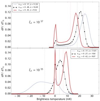
Figure 10: Brightness-temperature PDF for redshifts (corresponding to $\bar{x}_{\mathrm{ion}}=$[0.17,0.28,0.43]) associated with the local maximum feature seen in the skewness of the $\zeta_{\textsc{x}}=10^{55}$ model for: $\zeta_{\textsc{x}}=10^{57}$ in the top plot (where the zero peak corresponding to ionized pixels is separate from, and to the left of, the contribution from neutral regions); and $\zeta_{\textsc{x}}=10^{55}$ in the bottom plot (where the contribution from neutral regions is merged with that of the zero peak). Statistics are calculated from maps resolved to 4 Mpc, and $\alpha=1.5$ for all models.

3.2.2 The impact of heating on interpreting signatures of reionization

Following the X-ray heating-dominated phase, discussed in Section 3.1, we see a rapid drop from the X-ray heating peak at low ionized fractions (in agreement with the findings of Mesinger et al. 2013). If X-ray heating occurs relatively late as in the $\zeta_{\textsc{x}}=10^{55}$ model, the impact is dramatic as the drop from the heating peak occurs during UV-driven reionization (occurring at $\bar{x}_{\rm ion}<0.3$). Fig. 10 shows the PDFs during this phase. Unlike the $\zeta_{\textsc{x}}=10^{57}$ model (where there is a clear distinction between a positive brightness-temperature distribution and a sharp spike at $\delta T_{\rm b}=0$), the brightness-temperature distribution of the $\zeta_{\textsc{x}}=10^{55}$ PDF extends to negative temperatures. As a result, the contributions of neutral and ionized regions to the PDF are no longer distinct in brightness temperature. This reduces the variance and alters the skewness evolution, which exhibits a local maxima as the skewness tends to zero when $\overline{\delta T}_{\rm b}\sim 0$ in neutral regions.

Such signatures provide an opportunity to constrain the nature and timing of X-ray heating. However they also complicate interpretation of the variance and skewness during reionization, impacting our ability to constrain reionization using these moments. For example, Patil et al. (2014) fit a function with a single peak to the variance of mock data, in order to constrain parameters of reionization. Such an approach would return misleading constraints, especially if late X-ray heating occurred.

Ghara et al. (2015) note this fact and suggest to use either a three peak model (to model reionization, heating and coupling peaks) or a redshift cut-off. A redshift cut-off requires either prior knowledge on the timing of heating and reionization and/or throwing away information. The data itself could be used to provide a prior on where a redshift cut should be made (for example, model selection could be used to infer whether a three, two or one peak model best describes the data in hand and where the transitions from one to the next occur). However, this would still be misleading in the $\zeta_{\textsc{x}}=10^{55}$ model, as the drop from the heating peak occurs over redshifts for which the ionized fraction is $\sim 0.25$ and the peak (usually associated with the mid point of reionization) is at ionized fractions of between $0.6$ and $0.7$. We therefore conclude that it would be prudent to use a parameter estimation approach that uses simulations to capture such subtleties. Unfortunately, this is particularly challenging as simulations that include spin-temperature fluctuations are computationally expensive. Similar considerations would be necessary in constructing models of the skewness along the lines of Patil et al. (2014).

These arguments are also relevant to MCMC parameter estimation using simulations that assume the spin temperature is saturated, such as that of Greig & Mesinger (2015) (who consider the power spectrum rather than the variance). It would be interesting to test the code they describe (21cmmc) against a mock dataset generated from models similar to those we describe here to quantify the potential bias we would suffer from ignoring the spin temperature in performing parameter estimation.

4 Observational prospects

To consider the effect of instrumental noise and foregrounds, we make use of the publicly available code 21cmsense (Pober et al., 2014, 2013). We refer the readers to the 21cmsense literature for details, but we will describe the main points for completeness.

There are two main contributions to the error on the power spectrum: thermal noise and sample variance. At lower redshifts shot noise of the distribution of H i must also be considered, but this term is neglected in this analysis as it is found to be a sub-dominant effect, even after reionization (see Pober et al. 2013). Pober et al. (2013, 2014) calculate the noise for the $k$-mode measured by each individual baseline. As such, for a given redshift, the power spectrum may be calculated by application of an inverse-variance-weighted summation, for which the optimal estimator of the total noise error is,

$$\begin{split}\delta\Delta^{2}(k)=\left\{\sum_{i}\frac{1}{[\Delta^{2}_{\mathrm{\textsc{n}},i}(k)+\Delta^{2}_{\mathrm{\textsc{sv}},i}(k)]^{2}}\right\}^{-\frac{1}{2}}\,.\\ \end{split}$$ (12)

The thermal noise contribution for a $k$-mode labelled by $i$ is given by $\Delta^{2}_{\mathrm{\textsc{n}},i}(k)=X^{2}_{i}Y_{i}[k_{i}^{3}/(2\pi^{2})][\Omega_{i}/(2t_{i})]T^{2}_{\mathrm{sys}}$. In this expression $X^{2}Y\,[h^{-1}\,$Mpc$]$ translates observed units into cosmological distances; $\Omega_{i}[\mathrm{steradians}]$ is the solid angle of the primary beam for a given baseline; $T_{\mathrm{sys}}[\mathrm{K}]$ is the system temperature, a combination of the sky and receiver temperatures, (i.e. $T_{\mathrm{sys}}=T_{\mathrm{rec}}+T_{\mathrm{sky}}$); and $t_{i}[\mathrm{hours}]$ is the integration time for a given mode. The effect of the Earth’s rotation (relevant to a drift-scan observation mode) is taken into account when calculating the noise on an individual mode; i.e. different baselines may observe the same mode at different times which increases the integration time and therefore reduces thermal noise (for a similar reason, redundant baselines are useful). The sample variance error $\Delta^{2}_{\mathrm{\textsc{sv}},i}(k)$ is equivalent to the 21-cm power spectrum for that mode at a given redshift, i.e. $\Delta^{2}_{\mathrm{\textsc{sv}},i}(k)=\Delta^{2}_{21,i}(k)=k^{3}/(2\pi^{2})P_{21}(k)$ where $P_{21}(k)$ is the 21-cm brightness-temperature power spectrum.

As well as needing to beat down this error term, there is also the issue of foregrounds which swamp the signal by several orders of magnitude. By considering the Fourier transform along the frequency axis of each mode independently (effectively measuring the delay in signal arrival time between the two interferometer elements that make up a baseline), Parsons et al. (2012) find that the spectrally smooth nature of foregrounds mean that their contribution will be confined to the region of delay space containing the maximum delays for a given baseline (confining them to be below an ‘horizon limit’). On the other hand, the 21-cm signal should exhibit unsmooth spectral characteristics so that some contribution from the cosmological signal will be observed with smaller delays (i.e. above the ‘horizon limit’). This motivates the definition of $k_{\parallel,\mathrm{min}}$ and $k_{\perp,\mathrm{min}}$ below which foregrounds will dominate. Because of the frequency dependence of interferometer baselines, this ‘horizon limit’ drifts to increasing values of $k_{\parallel}$ with baseline length (i.e. with increasing $k_{\perp}$) producing a ‘wedge’ of foreground contamination in $k_{\parallel,\mathrm{min}}$-$k_{\perp,\mathrm{min}}$ parameter space. Mathematically the $k_{\parallel,\mathrm{min}}$ ‘horizon limit’ may be described as (Parsons et al., 2012),

$$\begin{split}k_{\parallel,\mathrm{hor}}=\left(\frac{1}{\nu}\frac{X}{Y}\right)k_{\perp}\,,\\ \end{split}$$ (13)

where $X$ and $Y$ convert angle and frequency to co-moving distance respectively.

There are two main approaches to dealing with the problem of foregrounds. One approach is to exploit the confinement of foregrounds to the ‘horizon limits’ described above and essentially ignore modes that fall outside of EoR window (the region of $k_{\parallel}$-$k_{\perp}$ space bounded by the ‘horizon limits’); see Datta et al. 2010; Vedantham et al. 2012; Morales et al. 2012; Thyagarajan et al. 2013; Hazelton et al. 2013; Liu et al. 2014b. When performing an inverse-variance-weighted (IVW) summation over $k$-modes, this is equivalent to assigning infinite noise to modes that fall outside the EoR window. In parallel, there is a great deal of effort going into actively removing foregrounds from observations; these exploit the smooth spectral characteristics of foregrounds to identify and remove their contribution (see Wang et al. 2006; Liu & Tegmark 2011; Paciga et al. 2011; Petrovic & Oh 2011; Chapman et al. 2012; Cho et al. 2012; Shaw et al. 2014).

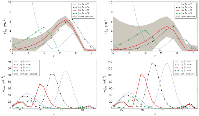
Figure 11: Inverse-variance weighted variance as measured when foregrounds are removed. LOFAR (Top-left); MWA (top-right); HERA (bottom-left); SKA (bottom-right). In the interest of brevity we do not explicitly consider PAPER’s performance, but PAPER-128 should be comparable in sensitivity to MWA for measuring the inverse-variance weighted variance. In this best case scenario all instruments are seen to be capable of constraining reionization; HERA and SKA would also tightly constrain WF-coupling and X-ray heating.

Although the effectiveness of foreground removal has yet to be proved (for example, the impact of the frequency dependent nature of the instrument on the effectiveness of these removal techniques has yet to be established), we consider optimistically that it will be possible to remove foregrounds (described by ‘remove’ in the plots of IVW-brightness-temperature variance as a function of redshift in Fig. 11), and so reduce the wedge’s extent to the edges of the instrument’s field of view. In considering foreground avoidance (described as ‘avoid’ in the plots of Fig. 12), we assume that the spectral structure of the foregrounds only extend by $\Delta k_{\parallel}=0.1h\,$Mpc^-1 beyond the wedge described by Equation 13 (in line with the predictions of Parsons et al. 2012). For both foreground models we assume that baselines sampling the same $k_{\perp}$ can be combined coherently.

Table 1: Summary of the instrumental properties we assume in calculating our errors. We assume a bandwidth of $8\,$MHz and an integration time of $1000\,$hours for all instruments. We use exact station locations for MWA and LOFAR from Beardsley et al. (2012) and van Haarlem et al. (2013) respectively (we also assume that each LOFAR HBA substation can be correlated independently to maximize redundant baselines). For HERA we assume 331 antenna in a closely packed hexagon as per Pober et al. (2013). Following Pober et al. (2013) and Greig & Mesinger (2015) we model SKA as a closely packed hexagon (to maximize redundancy) of 218 antenna out to $\sim 300$ m with a further 215 stations randomly distributed in an annulus from to $300$-$600$ m, 217 randomly placed stations in another annulus from 600-1000 m, and 216 randomly placed in an annulus covering 1000-2000 m from the centre of the array.

Parameter	LOFAR	MWA	HERA	SKA-1
Number of stations	48	128	331	866
Element size [m]	30.8	6	14	35/$\sqrt{2}$
Collecting area [m2]	35,762	896	50,953	416,595
Receiver T [K]	140	440	100	40

We perform an IVW summation over the power spectra measured by an instrument (using errors from 21cmsense and the instrumental properties described in table 1) to get constraints on the brightness-temperature variance. The 1-$\sigma$ error on the IVW variance is estimated by $[\sum_{i}(1/\delta\Delta^{2}_{i})^{2}]^{-\frac{1}{2}}$. An inverse-variance-weighted sum over the dimensionless power spectrum ($\Delta^{2}_{i}$) at different $k_{i}$ is only an unbiased estimator if the noise is Gaussian distributed with zero mean and the power is approximately flat (i.e. $\Delta^{2}_{i}=\Delta^{2}$ for all $i$) so that $\langle\sum_{i}(\Delta^{2}_{i}+n_{i})(1/\delta\Delta^{2}_{i})^{2}/\sum_{i}(1/\delta\Delta^{2}_{i})^{2}\rangle=\Delta^{2}$. Of course this is not strictly true as there is important evolution in the shape of the power spectrum with $k$. As such calculating $\sigma^{2}_{\mathrm{ivw}}=\sum_{i}\Delta^{2}_{i}(1/\delta\Delta^{2}_{i})^{2}/\sum_{i}(1/\delta\Delta^{2}_{i})^{2}$ means that $\sigma^{2}_{\mathrm{ivw}}$ is sensitive to the details of the noise, which is in turn sensitive to the details of the instrument. The limited resolution of the instruments means that the power contribution from large $k$ is totally suppressed; it is this that recovers the characteristics of the variance seen in our $\sigma^{2}_{\mathrm{ivw}}$ statistic. Similarly, the IVW-variance is sensitive to the foreground model we assume; the presence of a foreground-corrupted wedge means that power from the associated $k$ modes will be suppressed in calculating $\sigma^{2}_{\mathrm{ivw}}$. As is clear from the differing amplitudes between the plots of Fig. 11 and those of Fig. 12, the level of foreground corruption can seriously impact the amplitude of the variance. We must therefore be very careful when interpreting this statistic quantitatively from observations. The power spectra measured from $k$-modes inside the EoR window should not suffer from this issue. The qualitative nature of the variance’s evolution is insensitive to the foreground corruption we consider here and could therefore be useful for constraining coupling, X-ray heating and reionization.

We find that the first-generation instruments will only be able to constrain our models using the variance if foreground removal is possible. If so, then as is clear from the top row of plots in Fig. 11, both LOFAR and MWA will be able to constrain reionization and would also be sensitive to late X-ray heating. However, using foreground avoidance LOFAR could be sensitive to models in which reionization ends later than our models assume, but will more likely be limited to setting upper limits (see the top plot of Fig. 12). Note that because of the maximal redundancy of its baselines, the next phase of PAPER (consisting of 128-elements, see Ali et al. 2015) is only marginally less sensitive than MWA (see the appendix of Pober et al. 2014) despite having less than half the collecting area.

We again emphasise that our fiducial reionization model is optimistic, and so first-generation instruments may struggle more than is suggested by our analysis. Furthermore, due to the presence of sinks in the IGM the variance may be up to a factor of two smaller than the models of this paper predict. If extreme levels of remnant H i in galaxies are present then the variance will be reduced even further (Watkinson et al., 2015). Such reduction of the variance could make it difficult for first-generation instruments to do more than place upper limits, even if foregrounds can be removed. However, the IVW-variance will inevitably have smaller errors than the power spectrum at a given $k$ and therefore, first-generation instruments would do well to exploit it in their quest to make a first detection.

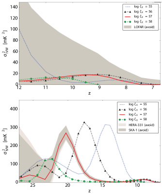
Figure 12: Inverse-variance weighted variance as measured from the foreground-free EoR window (i.e. by assigning infinite noise to power from foreground corrupted modes) by LOFAR (top), as well as by HERA and SKA (bottom). In this worst case scenario, LOFAR will be limited to placing upper bounds on the EoR, while HERA and SKA could still tightly constrain the EoR. HERA and SKA will still be able to constrain X-ray heating, but not WF-coupling.

Under the same assumptions, next-generation instruments such as SKA and HERA will be able to tightly constrain the variance for the coupling, heating and reionization epochs (as seen in the bottom plots of Fig. 11). Note that the IVW variance exhibits three distinct peaks corresponding to WF coupling, X-ray heating, and reionization; it does not exhibit the plateau between WF coupling and X-ray heating as seen in the standard variance (i.e. that measured from a clean simulated box). Even if foreground removal proves intractable then the foreground-avoidance technique will return strong constraints on the heating and reionization epochs (see the bottom plot of Fig. 12). Sinks in the IGM will not stop these next-generation instruments from returning strong constraints on the EoR using the moments. However, extreme levels of residual H i can qualitatively alter the evolution of the moments from that described in this paper (Watkinson et al., 2015).

We use the approach detailed in Watkinson & Pritchard (2014) to approximate instrumental errors on the skewness, this approach assumes that foregrounds can be perfectly removed and approximates instrumentals by smoothing and re-sampling pixels to match the resolution of the telescope. We plot the dimensional skewness as a function of both ionized fraction and redshift in Fig. 13. These errors should be viewed as optimistic estimates and will likely be quite a bit larger. As an illustration, if we compare the errors on the variance as calculated by Watkinson & Pritchard (2014) with those predicted for the IVW variance, we find its S/N is a factor of order 3 worse if foregrounds can be removed; if foreground avoidance is necessary then S/N can be 20 - 50 times worse.

We see that it will be possible to use the skewness to constrain models of late X-ray heating, possibly with LOFAR but certainly with the next-generation instruments. Therefore this presents an excellent opportunity for these telescopes to constrain a fundamental property of the Universe’s evolution, namely the relative timing of WF coupling, X-ray heating, and reionization.

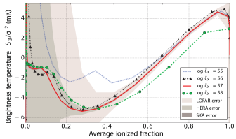
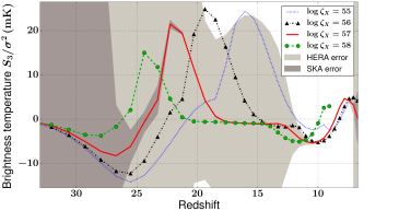
Figure 13: Dimensional skewness as a function of ionized fraction (top) and redshift (bottom) from brightness-temperature maps smoothed to a radius of 10 Mpc (top). Errors (shaded from dark to light for SKA, HERA and LOFAR respectively) correspond to approximate instrumental errors only and are therefore optimistic estimates. Whilst the first-generation instruments will struggle to extract useful constraints from this statistic, the skewness measurements from HERA and SKA will return vital constraints on the EoR. When we examine this statistic as a function of redshift (bottom), we find that SKA will also be able to tightly constrain X-ray heating with the skewness, but that HERA will not be sensitive to the skewness beyond the EoR.

5 Discussion

There are several approximations made in 21CMFAST that may have important repercussions; in particular the code assumes average properties of the IGM in calculating the X-ray mean free path. This is most important during the later stages of reionization when large ionized regions will result in fluctuations of the X-ray mean free path between sight-lines in the box. The code also assumes either population II or III stellar spectra in its calculations of WF coupling, and does not account for the possibility of mixed populations, feedback effects or shot noise. The nature of these first stars (and of the remnants they leave when they die) is very uncertain. Recent simulations indicate that these first stars will be $10-100\,M_{\odot}$ and are expected to form in small clusters (e.g. Hirano et al. 2014; Greif et al. 2011). Formation of such population III stars rely primarily on cooling via molecular hydrogen, however they produce large amounts of Lyman-Werner radiation (which disassociate molecular hydrogen) and so are likely to stunt further formation of population III stars (e.g. Wise & Abel 2007; O’Shea & Norman 2008). Such large stars are also short lived, so it is not unreasonable (as is done in this work) to assume that population II stars will be the dominant driver of the processes discussed here. However, it is possible that these results are inaccurate during the very early phases of coupling when the very first stars form.

Whilst simulations such as 21CMFAST have been tested against numerical simulations during the EoR assuming that the spin temperature is saturated (see for example, Zahn et al. 2011 and Majumdar et al. 2014), there has not been equivalent tests of these when spin temperature fluctuations are included. This is mainly because numerical simulations with the necessary scale and resolution do not yet exist. The only numerical simulations that perform radiative-transfer in all of the relevant frequency bands are those of Baek et al. (2010). These simulation do not resolve haloes with mass below 10${}^{10}M_{\odot}$, therefore they do not resolve atomically cooling haloes. As such, all astrophysical processes are driven by more massive, and therefore more rare and biased, haloes than is to be expected in reality. It is therefore not possible to draw direct comparison between Baek et al. (2010) and 21CMFAST . However, Mesinger et al. (2013) note that the qualitative evolution of the power spectrum at $k\sim 0.1$ of 21CMFAST (when including spin temperature fluctuations) is in agreement with the numerical simulations of Baek et al. (2010). We also find that the skewness of our late X-ray heating model ($\zeta_{\textsc{x}}=10^{55}$) qualitatively agrees with their S6 model, which is encouraging.

There are other processes that must be considered in parallel to spin temperature fluctuations. For example, and as already discussed, the presence of sinks could drastically reduce the variance. This reduction is due to residual signal in ionized regions and sub-pixel ionized regions. X-ray ionizations will occur in a more homogeneous fashion than UV ionizations and so will be responsible for partially ionizing regions outside of UV carved ionized regions. It therefore seems likely that the reduction of variance caused by X-ray ionizations will be in addition to that caused by sinks, i.e. they will further reduce the contrast between over and under-dense regions. The simulation of Sobacchi & Mesinger (2014) also incorporate UVB feedback which suppresses star formation, such feedback will clearly impact on both the Lyman-$\alpha$ and X-ray production. However, given the large amplitudes seen in the one-point statistics during the heating epoch, and that we have studied four orders of magnitude in the X-ray efficiency, it is unlikely that UVB feedback will have a dramatic effect beyond that seen here.

These examples (and the lack of numerical simulations with which to test 21CMFAST ) serve to illustrate the challenge we face in simulating the epochs of the first dawn and reionization. The results of this work should therefore not be considered conclusive and it is essential that we do more to understand how the statistics of the 21-cm moments are impacted by different physical processes (and their interplay).

6 Conclusion

In this paper, we have considered the sensitivity of one-point statistics of the 21-cm brightness temperature to fluctuations in WF coupling and X-ray heating, concentrating on the skewness and the variance. We use semi-numerical simulations to vary the efficiency at which X-rays are produced (to cover four orders of magnitude) and the spectral index of the X-ray SED (to encompass the range of observational constraints we have at low redshifts). From this study we establish that:

1. the location and amplitude of the global maxima in the redshift evolution of both the skewness and variance are sensitive to the X-ray production efficiency. The amplitude of this maximum in the variance is also sensitive to the hardness of the X-ray SED. This degeneracy may be broken, as the skewness is only sensitive to the X-ray production efficiency;

2. late X-ray heating causes the drop from the X-ray heating peak to occur at an ionized fraction of about a quarter rather than in the very early stages of reionization. In such a model, the turnover in the variance, usually associated with the mid-point of reionization, is shifted to higher ionized fractions. The evolution of the skewness is qualitatively different if X-ray heating occurs late, this provides a clean way to constrain such a model. The amplitude of the variance is greatly reduced in these models, which would make it more challenging for the first-generation instruments (such as LOFAR, MWA and PAPER) to make a detection of reionization using the variance;

3. the high-redshift heating peak must be allowed for in models used for parameter estimation from one-point statistics. If not our inferences may be very misleading. This is equally true for performing parameter estimation from the power spectrum;

4. X-ray ionizations reduce the amplitude of the variance. In most models we consider they reduce the variance by $\sim 10\%$ during the mid-phase of reionization; in the most X-ray efficient model, we find this reduction to be $\sim 25\%$.

We consider (for the first time to the authors’ knowledge) the variance as measured using foreground avoidance techniques. From this we find that the next-generation instruments such as HERA and SKA will return strong constraints on both reionization and X-ray heating, even if we are unable to remove foregrounds.

The findings of this paper will help us to correctly interpret future observations of the 21-cm brightness temperature; in particular they have important consequences for improving parameter estimation during reionization.

Appendix A Analytical expression for the skew of $\Delta\mu$

$$\begin{split}S_{3,\Delta\mu}&=3\left\langle\delta\left({\frac{T_{\textsc{cmb}}}{T_{\mathrm{s}}}}\right)^{2}\right\rangle-3\left\langle\delta^{2}{\frac{T_{\textsc{cmb}}}{T_{\mathrm{s}}}}\right\rangle+6\left\langle\delta\left({\frac{T_{\textsc{cmb}}}{T_{\mathrm{s}}}}\right)^{2}\right\rangle\\ &-\left\langle\left({\frac{T_{\textsc{cmb}}}{T_{\mathrm{s}}}}\right)^{3}\right\rangle-3\left\langle\delta\left({\frac{T_{\textsc{cmb}}}{T_{\mathrm{s}}}}\right)^{3}\right\rangle-3\left\langle\delta^{2}\left({\frac{T_{\textsc{cmb}}}{T_{\mathrm{s}}}}\right)^{3}\right\rangle\\ &+\left\langle\delta^{3}\right\rangle-3\left\langle\delta^{3}{\frac{T_{\textsc{cmb}}}{T_{\mathrm{s}}}}\right\rangle+3\left\langle\delta^{3}\left({\frac{T_{\textsc{cmb}}}{T_{\mathrm{s}}}}\right)^{2}\right\rangle\\ &-\left\langle\left(\delta{\frac{T_{\textsc{cmb}}}{T_{\mathrm{s}}}}\right)^{3}\right\rangle-6\left\langle{\frac{T_{\textsc{cmb}}}{T_{\mathrm{s}}}}\right\rangle\left\langle\delta{\frac{T_{\textsc{cmb}}}{T_{\mathrm{s}}}}\right\rangle\\ &+3\left\langle{\frac{T_{\textsc{cmb}}}{T_{\mathrm{s}}}}\right\rangle\left\langle\left({\frac{T_{\textsc{cmb}}}{T_{\mathrm{s}}}}\right)^{2}\right\rangle+6\left\langle{\frac{T_{\textsc{cmb}}}{T_{\mathrm{s}}}}\right\rangle\left\langle\delta\left({\frac{T_{\textsc{cmb}}}{T_{\mathrm{s}}}}\right)^{2}\right\rangle\\ &+3\left\langle{\frac{T_{\textsc{cmb}}}{T_{\mathrm{s}}}}\right\rangle\left\langle\delta^{2}\right\rangle-6\left\langle{\frac{T_{\textsc{cmb}}}{T_{\mathrm{s}}}}\right\rangle\left\langle\delta^{2}{\frac{T_{\textsc{cmb}}}{T_{\mathrm{s}}}}\right\rangle\\ &+3\left\langle{\frac{T_{\textsc{cmb}}}{T_{\mathrm{s}}}}\right\rangle\left\langle\left(\delta{\frac{T_{\textsc{cmb}}}{T_{\mathrm{s}}}}\right)^{2}\right\rangle-6\left\langle\delta{\frac{T_{\textsc{cmb}}}{T_{\mathrm{s}}}}\right\rangle^{2}\\ &+3\left\langle\left({\frac{T_{\textsc{cmb}}}{T_{\mathrm{s}}}}\right)^{2}\right\rangle\left\langle\delta{\frac{T_{\textsc{cmb}}}{T_{\mathrm{s}}}}\right\rangle+6\left\langle\delta{\frac{T_{\textsc{cmb}}}{T_{\mathrm{s}}}}\right\rangle\left\langle\delta\left({\frac{T_{\textsc{cmb}}}{T_{\mathrm{s}}}}\right)^{2}\right\rangle\\ &+3\left\langle\delta{\frac{T_{\textsc{cmb}}}{T_{\mathrm{s}}}}\right\rangle\left\langle\delta^{2}\right\rangle-6\left\langle\delta{\frac{T_{\textsc{cmb}}}{T_{\mathrm{s}}}}\right\rangle\left\langle\delta^{2}{\frac{T_{\textsc{cmb}}}{T_{\mathrm{s}}}}\right\rangle\\ &+3\left\langle\delta{\frac{T_{\textsc{cmb}}}{T_{\mathrm{s}}}}\right\rangle\left\langle\left(\delta{\frac{T_{\textsc{cmb}}}{T_{\mathrm{s}}}}\right)^{2}\right\rangle-2\left\langle{\frac{T_{\textsc{cmb}}}{T_{\mathrm{s}}}}\right\rangle^{3}\\ &-6\left\langle{\frac{T_{\textsc{cmb}}}{T_{\mathrm{s}}}}\right\rangle^{2}\left\langle\delta{\frac{T_{\textsc{cmb}}}{T_{\mathrm{s}}}}\right\rangle-6\left\langle{\frac{T_{\textsc{cmb}}}{T_{\mathrm{s}}}}\right\rangle\left\langle\delta{\frac{T_{\textsc{cmb}}}{T_{\mathrm{s}}}}\right\rangle^{2}\\ &-2\left\langle\delta{\frac{T_{\textsc{cmb}}}{T_{\mathrm{s}}}}\right\rangle^{3}\,,\\ \end{split}$$ (14)

References

- Ali et al. (2015) Ali Z. et al., 2015, preprint, arXiv:1502.06016
- Baek et al. (2010) Baek S. et al., 2010, A&A, 523, A4
- Beardsley et al. (2012) Beardsley A. P. et al., 2012, MNRAS.Lett., 429, L5
- Bond et al. (1991) Bond J. R. et al., 1991, ApJ, 379, 440
- Bowman & Rogers (2010) Bowman & Rogers, 2010, Nature, 468, 796
- Burns et al. (2012) Burns J. O. et al., 2012, Advances in Space Research, 49, 433
- Chapman et al. (2012) Chapman E. et al., 2012, MNRAS, 429, 165
- Chen et al. (2004) Chen X. & Miralda-Escude J., 2004, ApJ, 602, 1
- Cho et al. (2012) Cho J., Lazarian A., Timbie P. T., 2012, ApJ, 749, 164
- Choudhury et al. (2008) Choudhury T. R., Ferrara A., Gallerani S., 2008, MNRAS.Lett., 385, L58
- Datta et al. (2010) Datta A., Bowman J. D., Carilli C. L., 2010, ApJ, 724, 526
- Dijkstra et al. (2004) Dijkstra M., Haiman Z., Loeb A., 2004, ApJ, 613, 646
- Dillon et al. (2013) Dillon J. S. et al., 2013, 23, Phys.Rev.D, 89, 2
- Di Matteo et al. (2004a) Di Matteo T., Ciardi B., Miniati F., 2004a, MNRAS, 355, 1053
- Di Matteo et al. (2002b) Di Matteo T. et al., 2002b, ApJ, 564, 576
- Ewen & Purcell (1951) Ewen H. I., Purcell E. M., 1951, Nature, 168, 356
- Fabbiano (2006) Fabbiano G., 2006, ARA& A, 44, 323
- Fan et al. (2001) Fan X. et al., 2001, AJ, 122, 2833
- Field (1958) Field G. B., 1958, Proceedings of the IRE, 46, 240
- Field (1959) Field G. B., 1959, ApJ, 129, 536
- Friedrich et al. (2011) Friedrich M. M. et al., 2011, MNRAS, 413, 1353
- Furlanetto & Johnson Stoever (2010) Furlanetto S. R., Johnson Stoever S., 2010, MNRAS, 404, 1869
- Furlanetto et al. (2004a) Furlanetto S. R., Zaldarriaga M., Hernquist L., 2004a, ApJ, 613, 1
- Furlanetto et al. (2004b) Furlanetto S. R., Zaldarriaga M., Hernquist L., 2004b, ApJ, 613, 16
- Ghara et al. (2015) Ghara R., Choudhury T. R., Datta K. K., 2015, MNRAS, 447, 1806
- Gilfanov et al. (2004) Gilfanov M., Grimm H.-J., Sunyaev R., 2004, MNRAS, 347, L57
- Greif et al. (2011) Greif T. H. et al., 2011, ApJ, 737, 75
- Greig & Mesinger (2015) Greig B., Mesinger A., 2015, MNRAS, 449, 4246
- Harker et al. (2009) Harker G. J. A. et al., 2009, MNRAS, 393, 1449
- Hazelton et al. (2013) Hazelton B. J., Morales M. F., Sullivan I. S., 2013, ApJ, 770, 156
- Hickox & Markevitch (2007) Hickox R. C., Markevitch M., 2007, ApJ, 661, L117
- Hirano et al. (2014) Hirano S. et al., 2014, ApJ, 781, 60
- Hirata (2006) Hirata C. M., 2006, MNRAS, 367, 259
- Ichikawa et al. (2010) Ichikawa K. et al., 2010, MNRAS, 406, 2521
- Jenkins et al. (2001) Jenkins A. et al., 2001, MNRAS, 321, 372
- Lacey & Cole (1993) Lacey C., Cole S., 1993, MNRAS, 262, 627
- Lidz et al. (2008) Lidz A. et al., 2008, ApJ, 680(2), 962
- Liu & Tegmark (2011) Liu A., Tegmark M., 2011, Phys.Rev.D, 83, 103006
- Liu et al. (2014a) Liu A., Parsons A. R., Trott C. M., 2014a, Phys.Rev.D, 90, 023018
- Liu et al. (2014b) Liu A., Parsons A. R., Trott C. M., 2014b, Phys.Rev.D, 90, 023019
- Loeb & Furlanetto (2013) Loeb A., Furlanetto S. R., 2013, The First Galaxies in the Universe. Princeton University Press
- Madau et al. (1997) Madau P., Meiksin A., Rees M. J., 1997, ApJ, 475, 429
- Madau et al. (2004) Madau P. et al., 2004, ApJ, 604, 484
- Majumdar et al. (2014) Majumdar S. et al., 2014, MNRAS, 443, 2843
- McQuinn (2012) McQuinn M., 2012, MNRAS, 426, 1349
- Mellema et al. (2006) Mellema G. et al., 2006, MNRAS, 372, 679
- Mesinger & Furlanetto (2007) Mesinger A., Furlanetto S. R., 2007, ApJ, 669, 663
- Mesinger et al. (2011) Mesinger A., Furlanetto S. R., Cen R., 2011, MNRAS, 411, 955
- Mesinger et al. (2014) Mesinger A., Ewall-Wice A., Hewitt J., 2014, MNRAS, 439, 3262
- Mesinger et al. (2013) Mesinger A., Ferrara A., Spiegel D. S., 2013, MNRAS, 431, 621
- Mineo et al. (2012a) Mineo S., Gilfanov M., Sunyaev R., 2012a, MNRAS, 419, 2095
- Mineo et al. (2012b) Mineo S., Gilfanov M., Sunyaev R., 2012b, MNRAS, 426, 1870
- Mirabel et al. (2011) Mirabel I. F. et al., 2011, A&A, 528, A149
- Miralda-Escude (2003) Miralda-Escude J., 2003, ApJ, 597, 66
- Morales et al. (2012) Morales M. F. et al., 2012, ApJ, 752, 137
- Moretti et al. (2012) Moretti A. et al., 2012, A&A, 548, A87
- Oh (2001) Oh S. P., 2001, ApJ, 553, 499
- Oh & Mack (2003) Oh S. P., Mack K. J., 2003, MNRAS, 346, 871
- O’Shea & Norman (2008) O’Shea B. W., Norman M. L., 2008, ApJ, 673, 14
- Paciga et al. (2011) Paciga G. et al., 2011, MNRAS, 413, 1174
- Pacucci et al. (2014) Pacucci F. et al., 2014, MNRAS, 443, 678
- Parsons et al. (2012) Parsons A. R. et al., 2012, ApJ, 756, 165
- Patil et al. (2014) Patil A. H. et al., 2014, MNRAS, 443, 1113
- Petrovic & Oh (2011) Petrovic N., Oh S. P., 2011, MNRAS, 413, 2103
- Planck Collaboration et al. (2014) Planck Collaboration XVI, 2014, A&A, 566, A16
- Pober et al. (2013) Pober J. C. et al., 2013, AJ, 145, 65
- Pober et al. (2014) Pober J. C. et al., 2014, AJ, 782, 66
- Pober et al. (2015) Pober J. C. et al., 2015, preprint, arXiv:1503.00045
- Pritchard & Furlanetto (2006) Pritchard J. R., Furlanetto S. R., 2006, MNRAS, 367, 1057
- Pritchard & Furlanetto (2007) Pritchard J. R., Furlanetto S. R., 2007, MNRAS, 376, 1680
- Pritchard & Loeb (2008) Pritchard J. R., Loeb A., 2008, Phys.Rev.D, 78
- Rephaeli et al. (1995) Rephaeli Y., Gruber D., Persic M., 1995, A&A, 300, 91
- Santos et al. (2008) Santos M. G. et al., 2008, ApJ, 689, 1
- Shaver et al. (1999) Shaver P. A. et al., 1999, A&A, 345, 380-390
- Shaw et al. (2014) Shaw J. R. et al., 2014, ApJ, 781, 57
- Shimabukuro et al. (2014) Shimabukuro H. et al., 2014, preprint, arXiv:1412.3332
- Shull (1979) Shull J. M., 1979, ApJ, 234, 761
- Shull & van Steenberg (1985) Shull J. M., van Steenberg M. E., 1985, ApJ, 298, 268
- Sobacchi & Mesinger (2014) Sobacchi E., Mesinger A., 2014, MNRAS, 440, 1662
- Stacy et al. (2010) Stacy A., Greif T. H., Bromm V., 2010, MNRAS, 403, 45
- Storrie-Lombardi et al. (1994) Storrie-Lombardi L. J. et al., 1994, ApJ, 427, L13
- Swartz et al. (2004) Swartz D. A. et al., 2004, ApJS, 154, 519
- Thyagarajan et al. (2013) Thyagarajan N. et al., 2013, ApJ, 776, 6
- Tozzi et al. (2006) Tozzi P. et al., 2006, A&A, 451, 457
- Turk et al. (2009) Turk M. J., Abel T., O’Shea B., 2009, Science, 325, 601
- van Haarlem et al. (2013) van Haarlem M. P. et al., 2013, A&A, 56
- Vedantham et al. (2012) Vedantham H., Udaya Shankar N., Subrahmanyan R., 2012, ApJ, 745, 176
- Venkatesan et al. (2001) Venkatesan A., Giroux M. L., Shull J. M., 2001, ApJ, 563, 1
- Volonteri & Gnedin (2009) Volonteri M., Gnedin N. Y., 2009, ApJ, 703, 2113
- Wang et al. (2006) Wang X. et al., 2006, ApJ, 650, 529
- Watkinson & Pritchard (2014) Watkinson C. A., Pritchard J. R., 2014, MNRAS, 443, 3090
- Watkinson et al. (2015) Watkinson C. A. et al., 2015, MNRAS, 449, 3202
- Wise & Abel (2007) Wise J. H., Abel T., 2007, ApJ, 671, 1559
- Wouthuysen (1952) Wouthuysen S. A., 1952, AJ, 57, 31
- Wyithe & Morales (2007) Wyithe J. S. B., Morales M. F., 2007, MNRAS, 379, 1647
- Zahn et al. (2011) Zahn O. et al., 2011, MNRAS, 414, 727
- Zaldarriaga et al. (2004) Zaldarriaga M., Furlanetto S. R., Hernquist L., 2004, ApJ, 608, 622
- Zel’dovich (1970) Zel’dovich Y. B., 1970, A&A, 5, 84