Analogue White Hole Horizon and its Impact on Sediment Transport

Abstract:  
Motivated by the ideas of analogue gravity, we have performed experiments in a flume where an analogue White Hole horizon is generated, in the form of a wave blocking region, by suitably tuned uniform fluid (water) flow and counter-propagating shallow water waves. We corroborate earlier experimental observations by finding a critical wave frequency for a particular discharge above which the waves are effectively blocked beyond the horizon. An obstacle, in the form of a bottom wave, is introduced to generate a sharp blocking zone. All previous researchers used this obstacle.

A novel part of our experiment is where we do not introduce the obstacle and find that wave blocking still takes place, albeit in a more diffused zone. Lastly we replace the fixed bottom wave obstacle by a movable sand bed to study the sediment transport and the impact of the horizon or wave blocking phenomenon on the sediment profile. We find signatures of the wave blocking zone in the ripple pattern.

INTRODUCTION:
Ever since Hawking’s theoretical discovery [1] that Black Holes can radiate and Bekenstein’s proposal [2] of identifying the horizon area of a Black Hole with its entropy, there has been a paradigm shift in attempts to understanding quantization of gravity. In the framework of Jacobson [3] the above identification is put in a robust form where Einstein equations appear as equations of state, as in classical thermodynamics. Following Padmanabhan [4] and Verlinde [5] it now seems natural to understand gravity as an emergent phenomenon in a macroscopic sense. Gravity ceases to be a fundamental interaction like Electromagnetism and Weak and Strong interactions and it seems futile to try to gravity in the conventional way.

However, all of the above ideas rest on the physical existence of Hawking radiation and so far it has not been possible to observe it directly for the simple reason that for a typical astrophysical Black Hole the Hawking temperature is extremely tiny, (in fact numerically less than the CMB temperature). This has led researchers to look for experimentally accessible analogue systems where effective Black Hole metric can be simulated and dynamics of the relevant excitations in the effective Black Hole metric can be directly studied. The hope is to directly observe signatures of analogue Hawking radiation.

There appear to be several analogue systems where different aspects of the Hawking radiation phenomenon can be studied; optical systems [6] and the related Metamaterial scenario [7], Bose condensate [8], fluid system [9], in a specifically astrophysical use of the acoustic analogy [10]. (For a comprehensive review with references see [11, 12].) In the present paper we will focus on the analogue fluid model [9]. Unruh [9] had pioneered the idea that a wave-like disturbance impressed on a flowing fluid with non-uniform velocity is structurally same as the dynamics of an excitation in an effective curved spacetime. Hence a proper choice of flow and impressed wave can simulate a Black Hole-like effective metric leading to the formation of an analogue event horizon if the wave tries to penetrate an opposing background fluid flow that has a velocity larger than the effective wave velocity. This idea was experimentally tested by Rousseaux et.al [13] and by Weinfurtner et.al. [14] in a flume. An obstacle was placed on the bottom of the flume and it was seen that water waves could not overcome the opposing flow at a certain position above the obstacle. Hence a horizon was created beyond which the waves were absent and only the background flow of fluid remained. From a purely classical fluid dynamics context this phenomenon is quite common and observable in various natural settings [12]. A river mouth ending in the sea is an example of a natural white hole where the the river flow blocks the sea waves. The circular jump in the kitchen sink is a more controlled example. Another interesting example is the whale fluke-print . Indeed, it needs to be pointed out that the above phenomena are analogues of White Holes, the time reversed Black Hole, that is also a solution of the Einstein equation. In fact laboratory analogues, so far studied, are always analogue White Holes. So the novelty of the recent theoretical and experimental works lies in the interpretation of the results in the context of Analogue Hawking effect. The analysis of [14] showed that the waveform near the horizon consisted of the incoming long wavelength wave (that was impressed externally), and two short wavelength waves being swept back with the flow. Furthermore the amplitudes of the latter appeared in the exponential ratio as is true for Hawking radiation, that is predicted to be black body like. But most interestingly, one of the short wavelength waves had a negative frequency in the co-moving frame [13, 14] indicating directly the presence of mode mixing [15]. The interpretation of the experimental observation that waves are absent beyond the horizon is explained by noting that there is mode mixing at the horizon. The incoming long wavelength mode is converted to two short wavelength modes that are swept away with the flow and can not travel beyond the horizon.

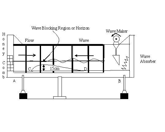
Figure 1: Schematic diagram of the flume with obstacle at blocking condition. AB = 10m is the straight portion of the flume. CD = 2.28m is the obstacle.

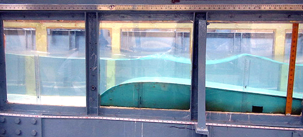
Figure 2: Wave blocking with obstacle in our flume

So far experimental studies in analogue fluid models in the context of Hawking effect have been confined to the study of the water surface profile. The real space water surface is Fourier transformed to analyze the contribution of various modes and their individual strengths. Subsequently the thermal nature of the Hawking radiation is verified. In the analogue scenario, this reduces to the study of conversion incoming shallow water waves to deep water waves at the wave blocking zone (or analogue horizon) that are swept along the flow. (For a discussion on water waves see eg. [16].) We, in the present experimental work, consider a rectangular channel or flume in which oppositely moving uniform flow of water and imposed wave-like disturbances are superimposed to produce the horizon (or blocking zone) beyond which the wave is absent. The schematic diagram of the experimental setup is presented in Figure 1. Here AB and CD represent the total flume and obstacle respectively and the uniform water flow is from A towards B. The actual wave blocking phenomenon in our flume is shown in Figure 2. We have observed the existence of a critical frequency of the incoming shallow water wave for a particular discharge, above which frequency the incoming wave is effectively blocked. This agrees with previous observations [17]. In these experimental setups the bottom of the flume consists of a fixed obstacle, referred to here as the bottom wave, (see Figure 1), that helps the wave blocking in two ways: on the one hand it increases the opposing background flow velocity at the top of the bottom wave and on the other hand it decreases the velocity of the incoming shallow water since the latter decreases as the water depth decreases. This allows the formation of a sharply defined blocking region (see Figure 2).

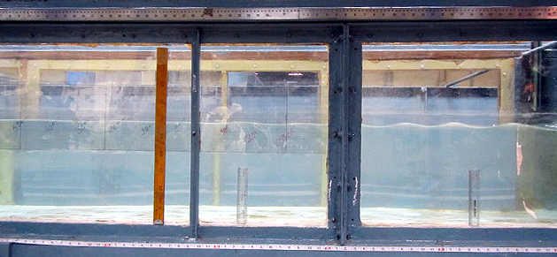
Figure 3: Wave blocking with no obstacle

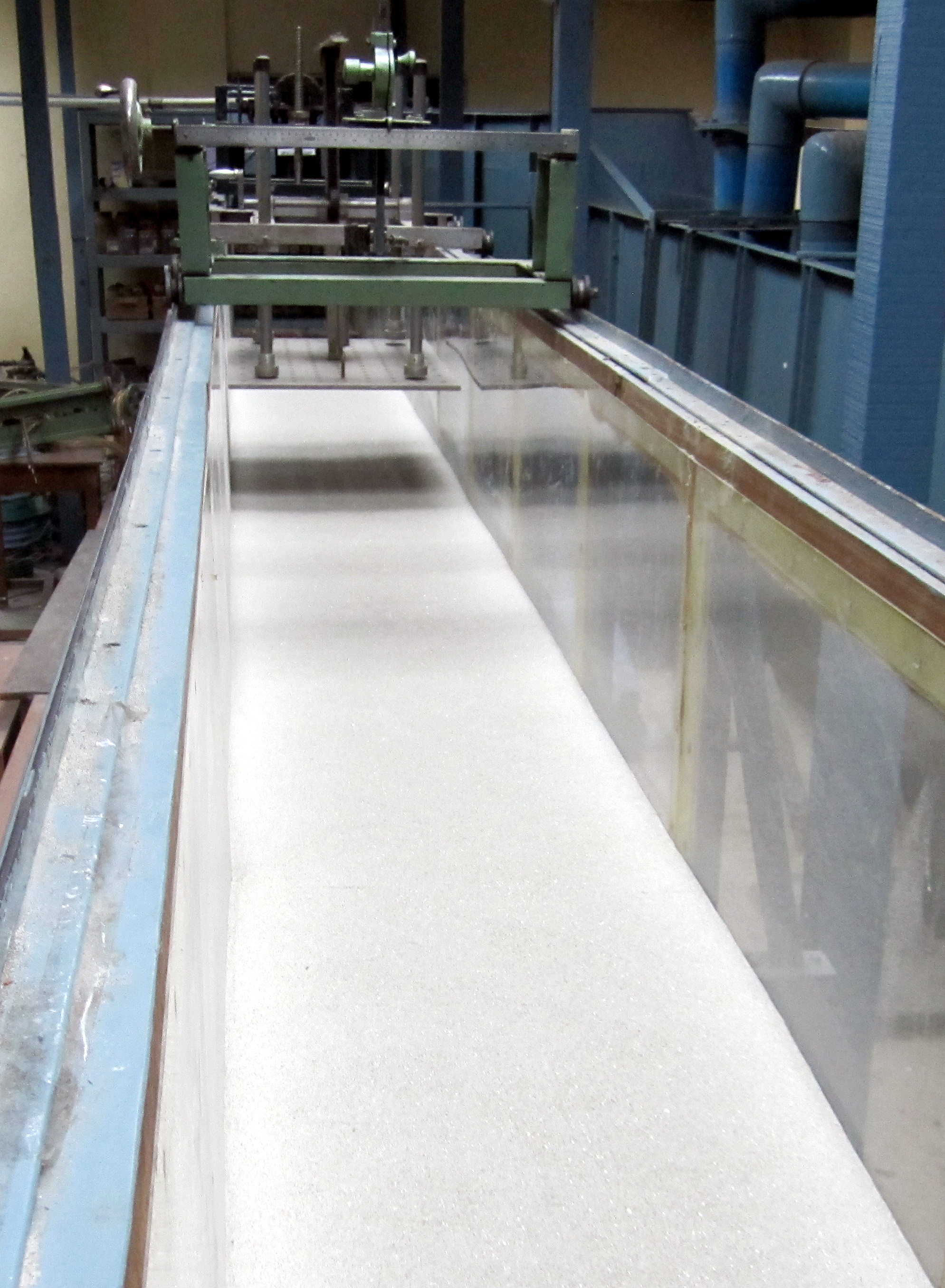
Figure 4: Flume with smooth sediment bed before experiment.

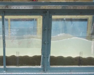
Figure 6: Wave blocking over the sediment bed

In our experiment, apart from the above, we have also ventured in an uncharted path: effect of wave blocking on sediment bed. This requires an important change in the experimental setup that is the bottom wave obstacle is removed and instead the flat bottom of the flume is covered with sand that acts as the sediment bed. In absence of the bottom wave the blocking region becomes slightly diffuse although it is still clearly visible (see Figure 3 where effect of wave blocking in flume without the bottom wave obstacle or sediment is presented). Figure 4 shows a typical smooth bed with fine sediment particles before starting of an experiment. For ripples to appear in the sediment bed the flow discharge or effectively the fluid velocity has to be chosen in such a way that the bottom shear stress is slightly higher than the threshold value for the initiation of sediment movement at the undisturbed plane sand bed. We show the uniform ripple structure for a steady flow in Figure 5. We compare the bed profile where uniform ripples are formed by the uniform flow only (see Figure 5) with the bed profile where both flow and opposing wave interact to create the blocking zone (see Figure 6). We have found signatures of the blocking region on the sediment bed profile as demonstrated in Figure 7. Note that photograph in Figure 7 consists of about ten photographs of consecutive portions of the sediment bed which were later edited to combine together to make one single photograph. Figures 6 and 7 are the new and most important observations of the present work.

The paper consists of the following sections: In Section II we provide a brief outline of the mathematics involved that leads to the analogue gravity scenario in fluid mechanics. Section III describes the experimental setup. Section IV consists of our experimental findings on the presence of a critical frequency above which the incoming waves are effectively blocked. Here the flume includes the bottom wave obstacle and is without sediment. Section V is devoted to the new setup where we remove the bottom wave obstacle and instead include the sediment in the form of sand bed. The paper ends in Section VI with our conclusions and future prospects of the present work.

Section II: Mathematical framework of analogue gravity in fluid

The basic mathematical framework is quite straightforward (for details see [12]). The Euler equation for the non-dissipative fluid with velocity field ${{\bf v}}$ is

$$\frac{d{{\bf v}}}{dt}=\dot{{\bf v}}+({\bf v}.\mbox{\bf$\nabla$}){\bf v}=-\frac{\mbox{\bf$\nabla$}p}{\rho}+{\bf g}+\frac{{\bf f}}{\rho}$$ (1)

where $p$ is the pressure, ${\bf g}=-g\vec{e_{z}}$ the acceleration due to gravity and ${\bf f}=-\rho\mbox{\bf$\nabla$}_{\parallel}V^{\parallel}$ a horizontal and irrotational force in the $x$ direction ($\parallel$) driven by the potential $V^{\parallel}$ which is at the origin of the flow.

We assume the flow to be without vorticity and hence $\mbox{\bf$\nabla$}\times{\bf v}=0$ . We find $({\bf v}.\mbox{\bf$\nabla$}){\bf v}=(\mbox{\bf$\nabla$}\times{\bf v})\times{\bf v}+\frac{1}{2}\mbox{\bf$\nabla$}(v^{2})=\frac{1}{2}\mbox{\bf$\nabla$}(v^{2})$ with ${\bf v}=\mbox{\bf$\nabla$}\phi$ where $\phi$ is the velocity potential. Without loss of generality the background flow ${\bf v}_{B}$ is taken to be stationary, irrotational and horizontal: $\mbox{\bf$\nabla$}_{\perp}{\bf v}_{B}=0$, ${\bf v}_{B}={\bf v}^{\parallel}_{B}\rightarrow\mbox{\bf$\nabla$}_{\parallel}.{\bf v}_{B}=0$. A velocity perturbation $\delta v$ of the background flow ${\bf v}_{B}$ with a corresponding vertical displacement $\delta h$ is considered. For a curl free velocity perturbation $\delta v$ we define a corresponding perturbed velocity potential $\delta\phi$. We skip the details of deriving the boundary condition for the perturbing potential $\delta\phi$ [12] and introduce a Taylor series expansion for $\delta\phi$:

$$\delta\phi(x,y,z)=\sum\limits_{n=0}^{\infty}\frac{z^{n}}{n!}\delta\phi_{(n)}(x,y).$$ (2)

Following [9, 12] for the case of the wavelengths much smaller than the water depth, one can develop a wave equation for $\delta\phi_{(0)}$,

$$\partial_{t}^{2}\delta\phi_{(0)}+2({\bf v}^{\parallel}_{B}.\mbox{\bf$\nabla$}_{\parallel})\partial_{t}\delta\phi_{(0)}+({\bf v}_{B}^{\parallel}\otimes{\bf v}_{B}^{\parallel}-gh)\mbox{\bf$\nabla$}^{2}\delta\phi_{(0)}=0.$$ (3)

The above can be expressed as a Beltrami-Laplace equation,

$$\Box\delta\phi_{(0)}=\frac{1}{\sqrt{-g}}\partial_{\mu}(\sqrt{-g}g^{\mu\nu}\partial_{\nu}\delta\phi_{(0)})=0$$ (4)

with the identification of $g^{\mu\nu}$ as an inverse metric given by,

$$g^{\mu\nu}=\begin{pmatrix}1&\vdots&{\bf v}^{\parallel}_{B}\\ \ldots\ldots\ldots&.&\ldots\ldots\ldots\ldots\\ {\bf v}^{\parallel}_{B}&\vdots&{\bf v}^{\parallel 2}_{B}-ghI\end{pmatrix}$$ (5)

Again, defining $g^{\mu\nu}g_{\mu\sigma}=\delta^{\nu}_{\sigma}$ we get the metric $g_{\mu\nu}$, popularly referred to as the acoustic metric in the conventional Painlevé-Gullstrand form,

$$g_{\mu\nu}=\frac{1}{c^{2}}\begin{pmatrix}gh-{\bf v}^{\parallel 2}_{B}&\vdots&{\bf v}^{\parallel}_{B}\\ \ldots\ldots\ldots&.&\ldots\ldots\ldots\ldots\\ {\bf v}^{\parallel}_{B}&\vdots&-1\end{pmatrix}$$ (6)

where $c=\sqrt{gh}$, the velocity of water waves in shallow water, plays the role of the analogue of velocity of light. Thus the acoustic metric has a singularity when ${\bf v}^{\parallel}_{B}=\sqrt{gh}$ that is the flow velocity becomes equal to the wave velocity but in opposite direction to it.

The dispersion relation is obtained by substituting a plane wave disturbance of the form $\delta\phi_{(0)}\sim exp(i\vec{k}.\vec{x}-i\omega t)$. One finds

$$(\omega-\vec{k}.\vec{v}_{b})^{2}=ghk^{2}.$$ (7)

This is infact the shallow water wave limit of the full dispersion relation

$$(\omega-\vec{k}.\vec{v}_{B})^{2}=gktanh(kh).$$ (8)

Let us now come to the flume experiments.

Section III: Experimental setup

The test channel or Flume: The experiments were carried out in a specially designed recirculating flume (Figure 1) at the Fluvial Mechanics Laboratory, Physics and Applied Mathematics Unit, Indian Statistical Institute, Kolkata. Both experimental and recirculating channels of the flume are of the same dimensions (10 m long, 0.5 m wide and 0.5 m deep). The experimental walls of the flume are made of Perspex windows with a length of 8 m, providing a clear view of the flow. One centrifugal pump providing the flow is located outside the main body of the flume. The inlet and outlet pipes are freely suspended from the overhead structure. The outlet pipe is fitted with one bypass pipe and a valve, so that by adjusting the valve in the outlet, the flow can be controlled at a desired speed. The upstream end of the channel is divided into three subchannels of equal dimensions, and one honeycomb cage is placed at each end of the subchannels to ensure smooth, vortexfree uniform water flow through the experimental channel. An electromagnetic discharge meter with a digital display is fitted with the outlet pipe to facilitate the continuous monitoring of the discharge. Water depth is kept constant at a depth of 25 cm for all experiments and the hydraulic slope shows to be of the order of 0.0001. Thereafter, one obstacle like waveform structure made of smooth Perspex is fabricated in the laboratory and placed at the bottom of the flume for experiment. The angles of the stoss-side and lee-side slopes of the structure are approximately $35^{0}$ and $6^{0}$ respectively. The structure is 2.28 m long with a crest height of 15 cm and spans the entire width of the flume. The obstacle is painted with epoxy paint to make the surface smooth. Particular care is taken to design the obstacle to minimize or avoid the flow separation. Our obstacle is scaled with the obstacle of the experiment in [17].
Wavemaker: A piston type wavemaker is mounted at the downstream end of the flume to generate surface waves against the current (Figure 1). The wavemaker is fabricated in the institute workshop. Two six-inch wheels are fitted at the end of a spindle, which has got a gear in its middle position. One crank and shaft is connected at the rim end of each wheel. The shafts are allowed to pass through a guide to restrict their motion in vertical direction only. A triangular shaped six inch cylinder (closed at both ends) is fitted at the other ends of the shafts. When the spindle is rotated with the help of motor, the cylinder moves to and fro in the vertical direction. The wavemaker is placed in such a way that the triangular cylinder remained partially submerged in water when it is at its extreme positions: topmost and lowermost. This is done to avoid the generation of small unwanted waves and disturbances in the flow. The amplitude of oscillations is maintained at 11 cm. Oscillations are produced at a right angle to the steady unidirectional current, which leads to the surface waves propagating against the current. The wavemaker is fixed with a Variac (variable resistor) to control the frequency of oscillation. Calibration is made using tachometer for frequency variation. The coordinate system of the measurement is as follows: x positive downstream and z positive upward. As the flume used in the present study is a recirculating one, the generated surface waves may get recirculated with the flow, which may bring more complexity in the flow. To avoid this complexity, a wave absorber is placed further downstream behind the wavemaker. Here, the experiments are performed over a range of discharges and frequencies of upstream waves against the flow over the obstacle. For each flow discharge i.e. flow velocity over the obstacle, a critical frequency of counter-propagating shallow water waves generated from the wavemaker is observed for the occurrence of wave blocking on the lee side of the obstacle, that means, the effective white hole horizon is experimentally observed for a particular frequency under a given flow discharge. The conversion from the shallow water waves generated from the wavemaker with a frequency over the obstacle to the deep water waves occurs, when a counter current becomes sufficiently strong to block the upstream propagation of shallow water waves.

Section IV: Analogue White Hole and partial wave blocking below critical frequency

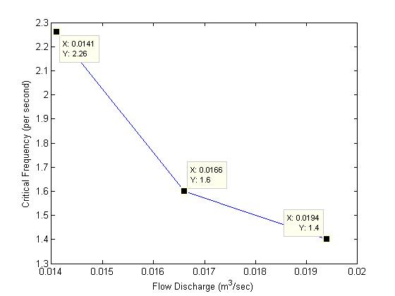
Figure 9: Critical frequency vs. discharge plot. The value of critical frequency decreases as the discharge increases. Here X and Y correspond to X-axis and Y-axis respectively.

In this section we provide the first set of observations of wave blocking or equivalently generation of the analogue White Hole horizon in experiments performed in our flume. Our aim is to show that for a given discharge, there exists a critical frequency above which imposed waves are blocked by the horizon. The blocking zone (or horizon) appears close to the crest of the obstacle, between the crest (inside positions C and D of Figure 1) and the wavemaker (position B in Figure 1). In order to observe the passage of waves beyond the horizon we fix our attention on the region close to the crest of the obstacle but in between positions A and C of Figure 1. We perform the experiment by keeping the discharge fixed and we increase the frequency of the wavemaker until there are effectively no fluctuations of the water surface in the observation point. There is no change if we increase the frequency of wavemaker still further. This indicates that for a given discharge a critical frequency exists above which the passage of waves over the obstacle are not allowed. However waves having frequency below the critical frequency can pass over the obstacle. This experiment is repeated for a number of discharges having different critical frequencies. From Figure 9 we also observe that the value of critical frequency decreases as the discharge increases.

The images of the amplitudes of a given frequency of counter propagating waves traveling over the obstacle were recorded by a camera. As all the data from the camera were in terms of pixel units, we converted those data to metric units. The recorded images of amplitudes were analyzed for a range of frequencies and discharges using digital imaging technique for better realization. Data were recorded for the variation of blocking frequencies with corresponding discharges.

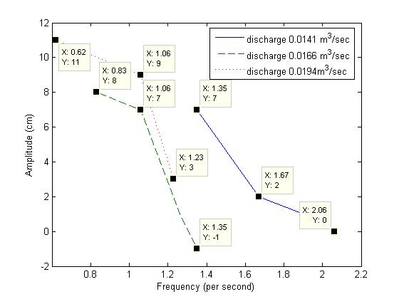
Figure 8: Amplitude vs. frequency plot for three different discharges. The value of frequency, (above which the amplitude abruptly vanishes), is called the critical frequency for that particular discharge. Here X and Y correspond to X-axis and Y-axis respectively.

Figure 8 shows the plots of wave amplitudes against the frequency for different discharges Q = $0.0141m^{3}/sec$, $0.0166m^{3}/sec$ and $0.0194m^{3}/sec$. As summarized in Table 1, notice that the blocking frequency decreases as the discharge increases. Furthermore, variations of amplitude of the wave with frequency for three different discharges can also be seen in Table 1. The amplitudes generically increase with increasing discharge. Our observations regarding critical frequency agree with earlier findings [17].

Section V: Sediment transport and effect of wave blocking on bed profile

An intensely active area of fluid dynamics research is sediment transport. In general when fluid bed is deformable the combined fluid-bed system results in a complicated non-linearly coupled system. The fluid flow directly affects the bed form and the latter, as a back reaction, can modify fluid flow. The study of sediment transport has wide practical applications in rivers and oceans and equally important is the study in laboratory flumes in a controlled environment. Studies of sediment transport from a modern perspective can be found in [18].

In laboratory flumes one generally performs experiments with initially smooth and flat sand beds, as in Figure 4. Bed forms with regular ripples and dunes are developed when sediment transport starts. The flow discharge or effectively the fluid velocity has to be chosen in such a way that the bottom shear stress is slightly higher than the threshold value for the initiation of sediment movement at the undisturbed plane sand bed, i.e. when there is no sand transport at the bed. Hjulstrom [19] suggested that there exists for each sand grain size a certain velocity, called critical velocity, above which it will experience erosion on the sediment bed. Subsequently, for initiation of sediment particle movement Shields [20] introduced a dimensionless quantity called shear stress, in terms of various relevant physical parameters of the system such as acceleration due to gravity, densities of the fluid and sediment, kinematic viscosity, etc. When shear stress exceeds the critical shear stress, the sediment motion begins to set in. As fluid flows over a flat sediment bed in a flume, the bed forms are generated along the flume surface. For example, Figure 5 shows photographs of the bed forms with small asymmetric ripples in an open channel flow. The bedform dimensions, such as amplitudes and wavelengths, depend on the flow velocity and the bed characteristics. This process seems to reach a steady state over a period of time and at each maximum velocity, the fully developed bedform (equilibrium category) seems to be evolved from an approximately steady uniform flow.

Interesting contributions along these lines were reported by Allen [21], where a very detailed account on bed forms and related features from a geologist/sedimentologists point of view is available. The most extensive experimental studies on bed forms were made by US Geological Survey at the Colorado State University (CSU). A summary of the data of all the flume experiments was presented by Guy et.al. [22]. Since then, several experimental investigations were performed under controlled conditions in laboratory flumes to study the bed form structures, sediment suspension and the influence of bed roughness over flat sediment beds of different composition [23].

In the present work we study the sediment bed topography and geometry of bed forms due to the the effect of upstream propagating waves against the flow. In particular we will concentrate on the nature of the bedform near critical frequency regime when wave blocking is in force on water surface.

In order to observe the sediment bed form structures a sand bed of thickness 10cm and of length 8m covering the entire width (50cm) of the flume is laid at the bottom of the flume. The median particle diameter of the sand is 0.25mm with a standard geometric deviation $\sigma_{g}$ = 0.685. The specific gravity of sediments used for the experiments is 2.65.

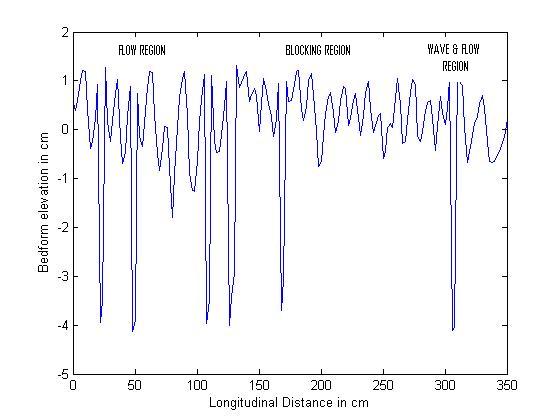
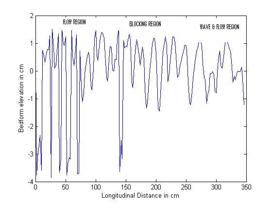
Figure 10: Actual ripple height vs. distance measured from A, as shown in Figure 1. Clearly the ripples on the left, near the flow dominated region, are higher than the ripples on the right near the horizon dominated region.

Series of experiments were conducted over the plane sediment bed to examine the effect of upstream propagating waves against the flow on the bed form structures that usually develop along the flow as regular ripples. In the first set of experiments we monitor the bed form structures only using the unidirectional flow of a given discharge over the plane sediment bed for a certain period of time to observe the uniform sand waves on the bed surface without the obstacle. In the second set of experiments we examine the bed profile when the counter propagating waves, (generated from the wavemaker), of fixed frequencies are superimposed on the flow. In particular we adjust the frequency so that the blocking condition is reached for a specific discharge and a horizon is formed. We repeat the process for different discharges and in each case we note the ripple pattern in the sediment throughout the sand bed when the blocking condition is reached. In all the cases a certain time, when the bed form gets nearly equilibrium state, the flow velocity is stopped and subsequently the bed elevations are measured at an interval of every 2cm from upstream to downstream along the center line of the flume covering the distance of about 3.5m. The instrument we use is Micro-acoustic Doppler velocimeter (ADV) made by Sontek, USA. Similar process is repeated to examine the effect of white hole horizon on the sediment bed form structures for different pairs of discharge and frequency. In Figures 10a and 10b we plot the exact (real space) ripple heights against distance for two different discharges, ie. $0.018m^{3}/sec$ and $0.019m^{3}/sec$. The bed elevation data analysis from Figures 10a and 10b suggests that there is a significant change in the bed form structures due to the wave blocking where the amplitude of upstream propagating waves is almost zero value. Our findings are summarized in Table 2.

Section VI: Conclusions and future prospects

In general, it is widely accepted that in a uniform open channel flow, when dimensionless shear stress exceeds the critical shear stress value the initiation of sediment motion starts on the flat bed surface. As the fluid velocity increases the bed shear stress increases and sediment transport starts where sediment is removed and transported locally. After a certain time it is observed that the sediment bed is changed completely forming a kind of regular asymmetric sand waves like ripples following the direction of the flow. As fluid flows over a flat sediment bed in a flume, due to the excess shear stress the bed forms are generated along the flume surface. The sediment is transported from the stoss-side and deposited in the lee-side of the ripple. The size and shape of ripples are uniform in a statistical sense and depends on the flow and bed features. Generically the ripples move downstream along the flow much slowly than the fluid. Indeed the sediment bed and fluid becomes a strongly coupled system with increase in flow velocity and results in an extremely complicated dynamical system even for a uniform fluid flow. There are various analytical models that attempt to predict the nature and motion of the ripples for a given flow but there are many important issues where consensus is not reached. (See [24] for an exhaustive study.) In our case, on top of the steady flow, there is the impressed gravity waves and to the best of our knowledge there is not much literature both in the form of experimental results or theoretical analysis. Some works on sediment transport have appeared where the impressed waves and the uniform flow both are in the same direction [25] but probably not much when the waves and uniform flow are in opposite direction.

Let us summarize our findings.
Our work can be divided in to two parts: (i) experiment with obstacle and without sediment and (ii) experiment without obstacle and with sediment.
(i) The first part of our work essentially reproduces early observations by [14, 17]. However our flume is of a considerably larger dimension than that used in [14] hence within the restrictions present in our instrumentation and laboratory setup it is not possible for us to reach the level of accuracy that is need to reproduce the experimental results found in [14]. On the other hand our flume is comparable in size with that of [17] so we have been able to derive quantitative estimates of the critical frequencies (of the imposed waves) for different discharges above which frequencies the waves are effectively blocked. The findings are summarized in Table 1. Three discharges are considered and for each one a blocking zone appears on top of the obstacle beyond which the wave amplitude decreases abruptly and effectively vanishes. Furthermore as the discharge increases the critical frequency value decreases showing that, as expected, the higher frequencies are blocked more easily and higher discharge is required to block lower frequencies.
(ii) In the second part of our work we use a distinctly different setup where the obstacle is replaced by a movable sediment bed consisting of sand. Our aim is to study sediment transport in presence of the horizon formation and blocking phenomenon. Specifically we have studied the ripple pattern on the sand bed (Figure 7) in detail after waiting for a sufficiently long time, (approximately four hours), to allow the sand bed to reach a state such that it is stable over time scales much larger than the time period of the waves. Comparing with the well-known ripple pattern in conventional uniform flows (without wave), Figure 5, we observe that in the present case the sediment bed is divided in to three sectors: in the flow dominated region (far away from the blocking zone but closer to the discharge source) the ripple structure for uniform flow prevails. The ripple structure is statistically uniform with asymmetrical shape ie. the ripples are sharper in the wave side and slopes more gently along the flow direction. Below the analogue white hole dominated blocking zone the sand ripples are more disorganized and on the average of lower height. Again in the wave-dominated region (far away from the horizon but closer to the wavemaker) the ripples are more symmetrical due to the interaction between the flow and wave force that tend to destroy the asymmetrical nature of the ripples and induces a more symmetrical shape. Therefore, the exploratory data analysis suggests that there is a transition in the bed form pattern in the flume with asymmetric ripples induced by the flow, followed by flat small sand bars in the blocking region and more symmetrical ripples in the wave dominated region. This suggests that the sediment bed may be segmented into three regions such as, the flow region at the upstream, blocking region, i.e. near analogue white hole horizon, and the wave region at the downstream respectively. Decreasing values of the standard deviation near the blocking condition in Table 2 also corroborates this.

Let us put our work in its proper perspective as it can have relevance in two different disciplines: On the one hand, in classical fluid dynamics it can be applied in practical situations having wave blocking zones where sediment bed profile plays an important role. If the analytic theory of sediment transport in the presence of opposing flow and wave is sufficiently developed its predictions can be tested in experimental setups like ours. On the other hand, in analogue gravity scenario, it can serve as an analogue of a different form of matter that couples with background gravity.

As a future work we wish to improve the statistics by making further observations with different discharge and frequencies. Another experimental aspect would be to study the turbulence phenomenon from the velocity spectrum of the fluid and sediment particles. Work is in progress along these directions.

Acknowledgements: It is indeed a pleasure to thank Silke Weinfurtner for early suggestions regarding the experimental setup. We are grateful to Koustuv Debnath and Satya Praksh Ojha for helpful discussions. The work of P. Das is funded by INSPIRE, DST, India.

Table 1:

Flow Discharge
0.0141$m^{3}/sec$		0.0166$m^{3}/sec$		0.0194$m^{3}/sec$
Frequency/sec	Amplitude(cm)	Frequency/sec	Amplitude(cm)	Frequency/sec	Amplitude(cm)
1.35	7	0.83	8	0.62	11
1.67	2	1.06	7	0.83	10
1.9	1	1.26	1	1.06	9
2.06	0	1.35	-1	1.23	3
2.26(blocking)	0	1.6(blocking)	-2	1.4(blocking)	-1

Table 2:

Actual Ripple Height in blocking condition measured from smooth bed							Same in only uniform flow
Flow($m^{3}/sec$)	Blocking Position		Towards Flow		Towards Wave Maker
	Mean	Standard	Mean	Standard	Mean	Standard	Mean	Standard
	Height(cm)	Deviation(cm)	Height(cm)	Deviation(cm)	Height(cm)	Deviation(cm)	Height(cm)	Deviation(cm)
0.0208	6.3269	0.5205	7.1064	1.348	6.7621	0.5744	6.8091	1.0962
0.0197	6.8413	0.769	7.3256	1.7491	6.8365	0.5425	8.301	0.8419
0.0183	6.4794	0.4249	6.856	1.4154	7.01	1.2608	8.0356	0.7111
0.0169	7.3173	0.5381	7.495	0.5536	7.2564	0.6033	8.5549	1.1738

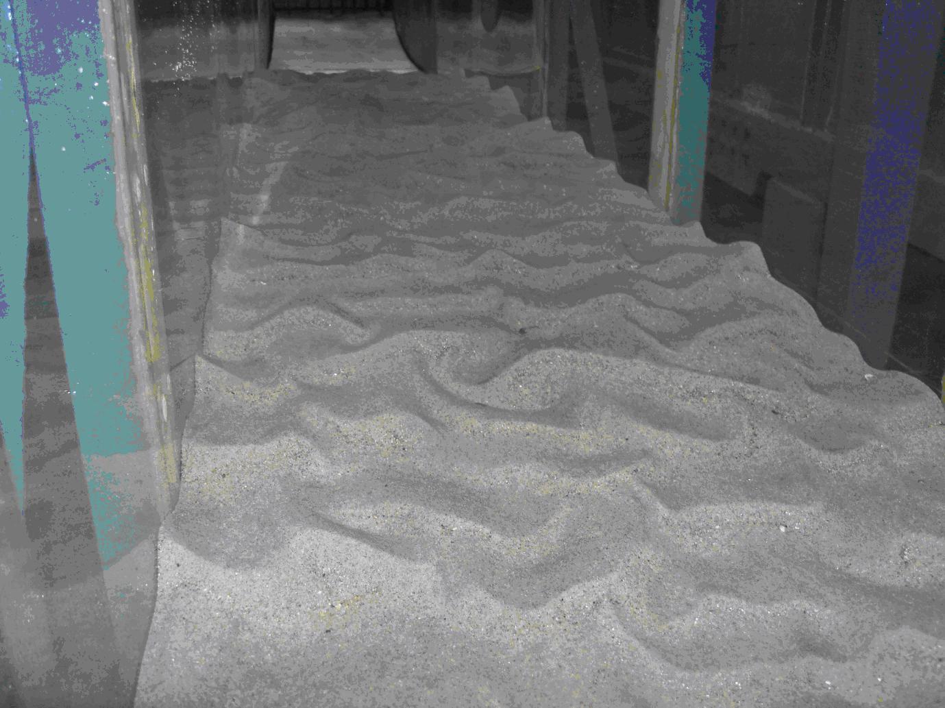
Figure 5: Ripples with only flow

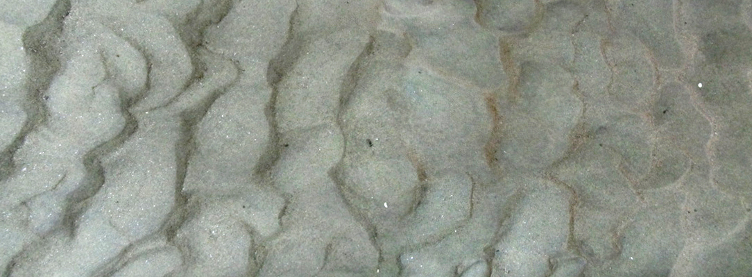
Figure 7: Effect of analogue White Hole horizon on sediment bed. The ripples are higher and more regular on the left side near the flow dominated region, similar to ripples with only uniform flow. Ripples on the right are small flat bar-like. The latter are below the horizon dominated region.

References

- [1] S.W. Hawking, Black hole explosions? , Nature, 248, 30 31, (1974); S.W. Hawking, Particle creation by black holes , Commun. Math. Phys., 43, 199 220, (1975).
- [2] J. D. Bekenstein, Phys. Rev. D7, 2333(1973).
- [3] T. Jacobson, (1995) Phys.Rev.Lett. 75 1260, [gr-qc/9504004].
- [4] T. Padmanabhan, Thermodynamical Aspects of Gravity: New insights , Rept. Prog. Phys., 73 (2010) 046901, [arXiv:0911.5004]; T. Padmanabhan, Gravity and the thermodynamics of horizons , Phys.Rept., 406 (2005) 49, [gr-qc/0311036].
- [5] E. P. Verlinde, arXiv:1001.0785 [hep-th].
- [6] U. Leonhardt, , Space-time geometry of quantum dielectrics , Phys. Rev. A, 62, 012111 1 8, (2000); F. Belgiorno, S. L. Cacciatori, G. Ortenzi, V. G. Sala, D. Faccio, Phys. Rev. Lett. 104, 140403 (2010); I. I. Smolyaninov and E. E. Narimanov, Phys. Rev. Lett. 105, 067402 (2010).
- [7] B. Reznik, Origin of the thermal radiation in a solid-state analogue of a black hole , Phys. Rev. D, 62, 044044 1 7, (2000); Subir Ghosh, Santanu K. Maiti, Spontaneous Photoemission From Metamaterial Junction: A Conjecture arXiv:1306.3748.
- [8] L.J. Garay, J.R. Anglin, J.I. Cirac, and P. Zoller, Sonic Analog of Gravitational Black Holes in Bose Einstein Condensates , Phys. Rev. Lett., 85, 4643 1 5, (2000). Related online version (cited on 31 May 2005): http://arXiv.org/abs/gr-qc/0002015.
- [9] W. G. Unruh, Experimental Black-Hole Evaporation ?, Phys. Rev. Lett., 46, 1351-1353 (1981).
- [10] T. K. Das, Analogous Hawking Radiation from Astrophysical Black Hole Accretion , (2004).
- [11] Carlos Barcel o, Stefano Liberati and Matt Visser, Analogue Gravity , Living Rev. Relativity, 8, (2005), 12.
- [12] G. Rousseaux, Lecture Notes for the IX SIGRAV School on ”Analogue Gravity”, Como (Italy), May 2011, arXiv:1203.3018.
- [13] G. Rousseaux, C. Mathis, P. Massa, T. G. Philbin and U. Leonhardt, New J. Phys., 10, 053015 (2008).
- [14] S. Weinfurtner, E. W. Tedford, M. C. J. Penrice, W. G. Unruh and G. A. Lawrence, Phys. Rev. Lett., 106, 021302 (2011); ibidClassical aspects of Hawking radiation verified in analogue gravity experiment. Arxiv: 1302.0375v1 [gr-qc]
- [15] R. Sch utzhold, and W.G. Unruh, Gravity wave analogues of black holes , Phys. Rev. D, 66, 044019 1 13, (2002); T. Jacobson, Phys.Rev. D53 (1996) 7082.
- [16] R. G. Dean and R. A. Dalrymple, (2000) Water Wave Mechanics for Engineers and Scientists, World-Scientifics, Singapore.
- [17] L. P. Fuve , F. Michel ,R. Parentani and G. Rousseaux ; Arxiv: 1409.3830v1.
- [18] Pierre Y. Julien, Erosion and Sedimentation, Cambridge University Press, 1995; R. J. Garde and K.G. Ranga Raju, Mechanics of Sediment Transportation and Alluvial Stream Problems, Wiley Eastern, 2000.
- [19] F. Hjulstrom (1935) The morphological activity of rivers as illustrated by rivers Fyris. Bull. Geol. Inst. Uppsala, Vol. 25 (Chapter III). (See W. H. Graf’s book on Hydraulics of sediment transport, Latest edition in 2010).
- [20] A. Shields (1936) Anwendung der Ahnlichkeitsmechanik und Turbulenzforschung auf die Geschiebebewegung, Mitteil. Preuss. Versuchsanst. Wasser. Erd., Schiffsbau, Berlin, no. 26. (See W. H. Graf’s book on Hydraulics of sediment transport, latest edition 2010).
- [21] J. R. L. Allen, (1968), Current Ripples, Elsevier, New York.
- [22] H. P.Guy, D. B. Simons, and E. V. Richardson (1966), Summary of alluvial channel data from flume experiments, U.S. Geol. Surv. Prof. Pap., 462 - 1, 1956 - 1961.
- [23] J.K. Ghosh, B.S. Mazumder, S. Sengupta,(1981) Methods of computation of suspended load from bed materials and flow parameters. Sedimentology 28, 781-791; K.Ghoshal, R. Mazumder, C. Chakraborty, and B. S. Mazumder (2013) Turbulence, suspension and downstream fining over a sand-gravel mixture bed. Int. J. Sed. Res.-Elsevier, 28 (2013) 194-209;B. S. Mazumder 1994, Grain size distribution in suspension from bed materials. Sedimentology, Vol. 41, pp. 271-277; J. G. Venditti, M. A. Church, and S. J. Bennett (2005) Bed form initiation from a flat sand bed. J. Geophys. Res., 110, F01009, doi: 10.1029/2004JF000149.
- [24] S. Dey, Fluvial Hydrodynamics, Springe-Verlag, 2014.
- [25] S.P. Ojha and B.S. Mazumder, J. Geophys. Res., 115, F04016, 2010; S.P. Ojha, Combined Wave-Current Flow; Doctoral thesis, Jadavpur University, Kolkata, India, 2008.