May 2015

Can gravitational microlensing
by vacuum fluctuations be observed?
S. Carlip
Department of Physics
University of California
Davis, CA 95616
USA

Abstract

Although the prospect is more plausible than it might appear, the answer to the title question is, unfortunately, “probably not.” Quantum fluctuations of vacuum energy can focus light, and while the effect is tiny, the distribution of fluctuations is highly non-Gaussian, offering hope that relatively rare “large” fluctuations might be observable. I show that although gravitational microlensing by such fluctuations become important at scales much larger than the Planck length, the possibility of direct observation remains remote, although there is a small chance that cumulative effects over cosmological distances might be detectable. The effect is sensitive to the size of the Planck scale, however, and could offer a new test of TeV-scale gravity.

1. Introduction

Quantum gravitational fluctuations of the vacuum are sometimes divided in two categories [1]. “Active” fluctuations are fluctuations of the spacetime geometry itself; beyond low orders of perturbation theory, their description presumably requires a full quantum theory of gravity. “Passive” fluctuations are fluctuations of the matter stress-energy tensor that induce fluctuations in the metric through the Einstein field equations. Their effect can be seen, for example, in the focusing or defocusing of a beam of light. A pencil of light—a congruence of null geodesics with an affinely parametrized null normal $\ell^{a}$—has a cross-sectional area $A$ whose change is characterized by the expansion

$$\theta=\frac{1}{A}\ell^{a}\nabla_{a}A=\frac{d\ }{d\lambda}\ln A,$$ (1.1)

where $\lambda$ is an affine parameter. The expansion, in turn, is governed by the Raychaudhuri equation [2, 3],

$$\frac{d\theta}{d\lambda}=\ell^{a}\nabla_{a}\theta=-\frac{1}{2}\theta^{2}-\sigma_{ab}\sigma^{ab}+\omega_{ab}\omega^{ab}-8\pi GT_{ab}\ell^{a}\ell^{b},$$ (1.2)

where $\sigma_{ab}$ is the shear, $\omega_{ab}$ is the vorticity, and the stress-energy tensor on the right-hand side encodes the effects of passive vacuum fluctuations. In particular, positive fluctuations focus, and thus temporary brighten, the beam.

Now, a typical quantum fluctuation of the stress-energy tensor at a length scale $L$ has a value $GT\sim\ell_{p}{}^{2}/L^{4}$, where $\ell_{p}$ is the Planck length. Naively, such fluctuations should be negligible at scales $L\gg\ell_{p}$. Their effects on the expansion $\theta$ were first considered at lowest order in [4], neglecting the nonlinear term in the Raychaudhuri equation, and the results were indeed found to be unobservably small. As Fewster, Ford, and Roman have demonstrated [5, 6], though, the distribution of fluctuations is highly non-Gaussian, with a sharp lower bound and an infinite subexponential positive tail. In such a setting, one must be very careful about expectations. It was shown in [5] that the non-Gaussianity greatly increases the probability of nucleating large objects such as primordial black holes and (perhaps) “Boltzmann brains,” and in [8] it was argued that one should expect dramatic effects at the Planck scale. In this paper I will investigate the possibility that such effects extend to a scale that might be directly observable. We shall see, unfortunately, that while fluctuations cause gravitational lensing at distances much larger than the Planck length, these are still almost certainly too small and short-lived to observe.

2. Vacuum fluctuations and “gambler’s ruin”

The strategy of Fewster et al. [5] was to compute vacuum correlation functions of products of many stress-energy tensors and to ask for the probability distribution for which these correlators were the moments. In two spacetime dimensions, recursion relations among correlators allow an exact computation, and the resulting probability distribution is unique [6]. In four dimensions, the computation is more difficult, but one can obtain an approximate distribution, along with very strong restrictions on the behavior of the tail [5].

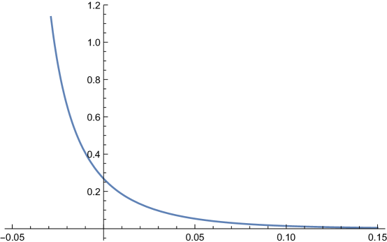
Figure 1: Probability distribution for vacuum fluctuations of electromagnetic energy

For vacuum fluctuations of the electromagnetic field, this distribution is shown in figure 1, in terms of the dimensionless stress-energy tensor at scale $L$,

$$x=\frac{16\pi^{2}}{\hbar}L^{4}T_{00}.$$ (2.1)

Note that the mass due to a vacuum fluctuations inside a sphere of radius $L$ is

$$\frac{Gm}{L}\sim\frac{1}{12\pi}\left(\frac{\ell_{p}}{L}\right)^{2}\,x.$$ (2.2)

We shall be mainly interested in the long positive tail of the distribution, which is well approximated by the equation

$$\mathit{Prob}(x)\sim c_{0}(x-x_{0})^{-2}e^{-a(x-x_{0})^{1/3}},\qquad c_{0}\approx.955,\ a\approx.963,\ x_{0}\approx-.0472,$$ (2.3)

where $x_{0}$ is the (calculated) lower bound on fluctuations.

The full quantum computation of the effects of these fluctuations, accounting for all of the nonclassical correlations, seems extremely difficult (although see [7] for a first effort). But we can obtain a reasonable approximation by treating the fluctuations as a classical stochastic process [8], with a random “kick” at each time interval $L$ selected from the distribution of Fewster et al.

Before proceeding, a few caveats are in order. First, the results of [5] were computed for the Minkowski vacuum, and may fail in regions of high curvature. We shall be looking at low curvature regions, though, so this should not be important. The results are also state-dependent; in particular, there are states in which there is no lower bound on vacuum energy along a null geodesic [9], and the argument that follows will fail for such states. The length scale $L$ is incorporated by smearing the stress-energy tensor over that scale, and the details of the distribution may depend on the choice of smearing function. (Fewster et al. use a Lorentzian average.) Finally—perhaps most seriously for this work—the relevant component of the stress-energy tensor in the Raychaudhuri equation (1.2) is a null-null component, while Fewster et al. have only computed distributions for the time-time component. I will assume that the behaviors are at least qualitatively similar, as they are in two dimensions [6]; given the tracelessness of the electromagnetic stress-energy tensor, one can argue that this must be true by symmetry considerations, but a more careful analysis would be useful.

Keeping in mind these caveats, we may proceed as follows [8]. Let us assume that the initial vorticity of our pencil of light is zero; it will then remain zero during propagation [3]. Then the only possible positive term on the right-hand side of the Raychaudhuri equation—the only term that can cause a defocusing—comes from the fact that vacuum fluctuations of $T_{ab}$ can be negative. But such defocusing fluctuations have a lower bound $x_{0}$, and if $\theta$ is negative enough, they cannot compete with the focusing caused by the nonlinear term $-\theta^{2}$. Hence if $\theta$ ever becomes sufficiently negative, it will necessarily be driven to $-\infty$.

This is essentially the phenomenon known in probability theory as “gambler’s ruin” [10]. The term has several meanings, but here the relevant statement is that if a player with a finite amount of money continues to bet against a banker with infinite resources, then no matter how favorable the odds, the player will eventually lose everything. In our context, the odds for defocusing are favorable—most vacuum fluctuations are negative. But the maximum amount of defocusing is limited, while focusing is not, so when a large enough positive fluctuation eventually occurs, the process becomes irreversible.

We may estimate of this effect as follows. At a fixed scale $L$, let

$${\bar{\theta}}=\sqrt{\frac{|x_{0}|}{\pi}}\frac{\ell_{p}}{L^{2}}.$$ (2.4)

It is easy to check that if $\theta<-{\bar{\theta}}$, the right-hand side of (1.2) is always negative, and the expansion will necessarily be forced down to $-\infty$. If $\theta>{\bar{\theta}}$, the right-hand side is also negative, and the expansion will be forced down to $\bar{\theta}$. For $-{\bar{\theta}}<\theta<{\bar{\theta}}$, on the other hand, the sign of the right-hand side is not fixed, and the expansion will vary as the vacuum fluctuates.

Now, most vacuum fluctuations are negative, and detailed simulations in two dimensions show that most of the time they drive the expansion to remain near its “maximum” $\bar{\theta}$. (Note that this is an extremely small value.) To force runaway focusing, we need a positive fluctuation large enough that in a time $L$,

$$\Delta\theta=\frac{d\theta}{d\lambda}L<-2{\bar{\theta}}.$$ (2.5)

From the Raychaudhuri equation, neglecting the effects of shear and assuming $L\gg\ell_{p}$, this requires that

$$x>4\sqrt{\pi|x_{0}|}\,\frac{L}{\ell_{p}}=x_{1}.$$ (2.6)

This is a fluctuation large enough that a sphere of radius $L$ contains a mass

$$\frac{m\,}{m_{p}}\gtrsim\frac{1}{3}\sqrt{\frac{|x_{0}|}{\pi}}\sim.13.$$ (2.7)

By (2.2), though, such a fluctuation is still weak, in the sense that

$$\frac{Gm}{L}\sim.13\frac{\ell_{p}}{L}\ll 1\quad\hbox{for $L\gg\ell_{p}$}.$$ (2.8)

While this method of estimation may seem rather crude, it has been shown to be extremely accurate in two dimensions [8]. Since fluctuations as large as (2.6) certainly can occur, runaway focusing is possible. Two questions remain, though: what is the physically relevant scale $L$, and, given such a scale, what is the probability of a positive energy fluctuation as large as (2.6)?

3. Probabilities

We begin with the more technical question: what is the probability of a fluctuation satisfying (2.6)? As long as $L/\ell_{p}$ is reasonably large, we will be in the tail, with a probability distribution (2.3). Thus

$$\mathit{Prob}(x>x_{1})\sim c_{0}\int_{x_{1}}^{\infty}(x-x_{0})^{-2}e^{-a(x-x_{0})^{1/3}}dx=3c_{0}a^{3}\Gamma[-3,a(x_{1}-x_{0})^{1/3}]$$ (3.1)

where $\Gamma$ is an incomplete gamma function. For large arguments, $\Gamma(k,u)\sim u^{k-1}e^{-u}$, so

$$\mathit{Prob}(x>x_{1})\sim\left(L/\ell_{p}\right)^{-4/3}e^{-\alpha(L/\ell_{p})^{1/3}}$$ (3.2)

where $\alpha$ is a number of order unity whose exact value will depend on such details as the choice of smearing function. Thus while the probability of a large fluctuation drops quickly as $L$ increases, it falls off considerably more slowly than one might first suppose.

Given such a fluctuation, we can next investigate the subsequent behavior of our pencil of light: at what distance does it focus? For this, we return to the Raychaudhuri equation (1.2). As a first approximation, which I will justify below, let us neglect any further fluctuations of the stress-energy tensor, as well as any contributions from the shear. Then the Raychaudhuri equation has the well-known solution

$$\frac{1}{\theta}=\frac{1}{\theta(0)}+\frac{1}{2}\lambda,$$ (3.3)

and focusing (i.e., $\theta\rightarrow-\infty$) occurs at at a distance

$$\lambda_{f}=-\frac{2}{\theta(0)}\sim\frac{2}{{\bar{\theta}}}\sim\beta\frac{L^{2}}{\ell_{p}}$$ (3.4)

where $\beta$ is a number of order unity.

This could be an underestimate: although negative energy fluctuations can never drive the expansion above $-{\bar{\theta}}$, they might slow its further descent. But this is a tiny effect. It is not hard to check from (1.2) that even with the inclusion of further negative energy fluctuations,

$$\lambda_{f}\leq\frac{2}{\bar{\theta}}\,\coth^{-1}\left|\frac{\theta(0)}{\bar{\theta}}\right|.$$ (3.5)

This is very close to (3.4) as long as $\theta(0)$ is even slightly smaller than $-{\bar{\theta}}$; for $\theta(0)=-1.01\,{\bar{\theta}}$, for example, it gives only a factor of $2.5$.

We thus have two observationally relevant scales: $L$, the scale that sets the size and duration of quantum fluctuations, and $\lambda_{f}$, the distance at which these fluctuations have a significant effect on the propagation of light. Note that in terms of $\lambda_{f}$, the probability (3.1) becomes

$$\mathit{Prob}(\lambda_{f})\sim\left(\lambda_{f}/\ell_{p}\right)^{-2/3}e^{-\gamma(\lambda_{f}/\ell_{p})^{1/6}}$$ (3.6)

where $\gamma$ is of order unity. Again, the probability of a “large” fluctuation falls off with size much more slowly than one might expect.

4. Microlensing

Suppose a vacuum fluctuation occurs along our line of sight as we observe a star. If the fluctuation is at a distance of order $\lambda_{f}$, it will focus the light, causing a momentary brightening much like that we observe in ordinary microlensing [11]. A fluctuation of characteristic size $L$, focusing over a distance $\lambda_{f}$, will subtend a solid angle $\Omega_{\hbox{\tiny\it vac}}\sim(L/\lambda_{f})^{2}\sim(\ell_{p}/L)^{2}$. A source of radius $r$ at distance $D$ will subtend an angle $\Omega_{\hbox{\tiny\it source}}\sim(r/D)^{2}$. For the fluctuation to focus a significant portion of the light, $\Omega_{\hbox{\tiny\it vac}}$ should not be much smaller than $\Omega_{\hbox{\tiny\it source}}$, so we must require

$$L\lesssim\frac{D}{r}\ell_{p},\quad\lambda_{f}\lesssim\left(\frac{D}{r}\right)^{2}\ell_{p}.$$ (4.1)

As an upper limit, we may be able to observe white dwarfs in the Large Magellanic Cloud [12], which would give an optimistic estimate of $D/r\sim\,10^{14}$, or

$$L\sim 10^{-21}\,\mathrm{m}.$$ (4.2)

This would correspond to a focusing length of $\lambda_{f}\sim 10^{-7}\,\mathrm{m}$; that is, lensing would require a fluctuation occurring within less than a micrometer of the telescope mirror. Moreover, although the probability (3.2) falls off more slowly than naive expectations, for a fluctuation of this size it is about $10^{-20000}$. This is not a promising setting for observation.

We could, of course, increase the probability by making $L$ smaller. This would also enlarge the solid angle $\Omega_{\hbox{\tiny\it vac}}$, boosting the number of potential sources. For $L\sim\,5\times 10^{5}\,\ell_{p}$, for instance, the probability of a fluctuation becomes about $10^{-42}$. While this is still a very small number, it is the probability for a fluctuation of size $L$ in a time $L/c\sim 5\times 10^{5}\,t_{p}\sim 10^{-38}\,\mathrm{s}$, corresponding to a rate of several events per day.

Unfortunately, though, while such fluctuations are large compared to the Planck length, they are still tiny compared to a typical wavelength of light. The geometric optics approximation implicitly assumed in the Raychaudhuri equation fails for scales that are small compared to the wavelength, and there is no reason to suppose that such fluctuations would have the same focusing effects. But even the scale $L\sim 10^{-21}\,\mathrm{m}$ of eqn. (4.2) corresponds to a photon with an energy on the order of $100\,\mathrm{TeV}$.

What is ultimately fatal to this idea, though, is the time scale of the fluctuations themselves. The “best case” (4.2) is a fluctuation that lasts $10^{-29}\,\mathrm{s}$. The case $L\sim\,5\times 10^{5}\,\ell_{p}$—about the largest value that gives a reasonable event rate—corresponds to a fluctuation lasting only $10^{-38}\,\mathrm{s}$. The prospects of observing a microlensing event of such a short duration seem dim indeed.

One possibility remains, though: the effects of vacuum fluctuations could accumulate over long distances. For photons with energies less than about $10^{-9}\,E_{p}$—even allowing for $\mathcal{O}(10)$ corrections in the exponent in (3.2)—the probability of a “large” fluctuation along a photon trajectory is nearly zero even at cosmological distances, so runaway focusing is not expected. Blurring of images and variations in luminosity may still occur, however. Borgman and Ford have studied this process for small fluctuations [4], and find that while the effects do accumulate, the variations in the expansion are of order $\ell_{p}{}^{2}/L^{3}$, again too small to see.

But one loophole may still be present. Borgman and Ford considered an approximation in which the nonlinearity of the Raychaudhuri equation could be neglected. But we know from [8] that near the Planck scale, negative energy fluctuations can quickly drive the expansion to the value $\bar{\theta}$ of eqn. (2.4), where the nonlinearities become important. For $L\gg\ell_{p}$ such a process would be slower, but it could still be important.

To obtain a rough estimate, consider a random walk induced by fluctuations of the typical size $\Delta(GT)\sim\pm\ell_{p}{}^{2}/L^{4}$, each lasting a characteristic time $L$. After $N$ steps, the average expansion will be

$$\langle\theta\rangle\sim\sqrt{N}\,\frac{\ell_{p}{}^{2}}{L^{3}},$$ (4.3)

which will be of order $\bar{\theta}$ when $N\sim(L/\ell_{p})^{2}$, that is, at a distance

$$d\sim\frac{L^{3}}{\ell_{p}{}^{2}}.$$ (4.4)

For a cosmological source at $d\sim 50\,\mathrm{Mpc}$, the nonlinear regime could be reached by fluctuations as large as $L\sim 10^{-15}\,\mathrm{m}$. This is still too small to see, but no longer quite as outrageously so—it corresponds roughly to the wavelength of a $1\,\mathrm{GeV}$ photon.

This is still too crude an estimate, for several reasons. First, the stochastic treatment of quantum fluctuations neglects correlations. Second, as stressed above, the real “random walk” is highly biased—step sizes and probabilities can be read from figure 1, and are not at all uniform. Third, the electromagnetic field does not give the only contribution to vacuum fluctuations; at the scales we are considering, even QCD fluctuations may be important. The first of these considerations will slow the diffusion process, requiring longer times to reach the nonlinear regime, but the second and third will almost certainly shorten the required time. If, in fact, the nonlinear regime can be reached, the effect of vacuum fluctuations can be much larger than the estimate of [4]; it will require future work to see whether this is possible.

5. Conclusion

Quantum fluctuations of vacuum energy are tiny, and one would not ordinarily expect them to have a detectable effect on the propagation of light. But their distribution is highly non-Gaussian, and exceptionally large fluctuations occur much more often than one would naively estimate. The estimates of the preceding section indicate that even averaged over a sphere with a volume $10^{17}$ times the Planck volume, “large” fluctuations may occur a few times a day. Moreover, the Raychaudhuri equation is nonlinear, amplifying the effect of such large fluctuations.

But the Planck length is very small. In the end, the non-Gaussian and nonlinear effects seem to require energies too high and times too short for us to detect. By adding more fields, one might shift exponents by factors of order a few, but even this is not likely to help. It remains possible, though, that the cumulative effects of fluctuations may be observable, not in microlensing but in fluctuations and “blurring” of images. It has also been suggested in [13], in a rather different context, that vacuum fluctuations might be visible in the integrated Sachs-Wolfe effect. A further investigation in the present context could be of interest.

Finally, these results might place new restrictions on “TeV-scale gravity” [14]. For a Planck mass of, say, $10\,\mathrm{TeV}$, the energies for runaway focusing discussed in the preceding section are reduced to about $20\,\mathrm{MeV}$. For the cumulative effects described at the end of that section, the changes are even more dramatic: for a smearing length $L\sim 700\,\mathrm{nm}$, comparable to the wavelength of visible light, the nonlinear regime could be reached in as little as about $100\,\mathrm{kpc}$. A more thorough analysis is again necessary, but this could give a significant new limit on TeV-scale gravity models.

Acknowledgments

This work was supported in part by Department of Energy grant DE-FG02-91ER40674.

References

- [1] L. H. Ford and C.-H. Wu, Int. J. Theor. Phys. 42 (2003) 15, arXiv:gr-qc/0102063.
- [2] A. Raychaudhuri, Phys. Rev. 98 (1955) 1123.
- [3] S. W. Hawking and G. F. R. Ellis, The Large Scale Structure of Space-Time (Cambridge University Press, Cambridge, 1973).
- [4] J. Borgman and L. H. Ford, Phys. Rev. D70 (2004) 064032, arXiv:gr-qc/0307043.
- [5] C. J. Fewster, L. H. Ford, and T. A. Roman, Phys. Rev. D85 (2012) 125038, arXiv:1204.3570.
- [6] C. J. Fewster, L. H. Ford, and T. A. Roman, Phys. Rev. D81 (2010) 121901, arXiv:1004.0179.
- [7] N. Drago and N. Pinamonti, J. Phys. A 47 (2014) 375202, arXiv:1402.4265.
- [8] S. Carlip, R. A. Mosna, and J. P. M. Pitelli, Phys. Rev. Lett. 107 (2011) 021303, arXiv:1103.5993.
- [9] C. J. Fewster and T. A. Roman, Phys. Rev. D67 (2003) 044003, arXiv:gr-qc/0209036.
- [10] J. L. Coolidge, Ann. Math. 10 (1909) 181.
- [11] B. Paczynski, Ap. J. 304 (1986) 1.
- [12] R. A. W. Elson et al., Ap. J. 499 (1998) L53, arXiv:astro-ph/9802117.
- [13] N. Afshordi and E. Nelson, arXiv:1504.00012.
- [14] N. Arkani-Hamed, S. Dimopoulos, and G. R. Dvali, Phys. Rev. D59 (1999) 086004, arXiv:hep-ph/9807344.