A low complexity algorithm for non-monotonically evolving fronts

Abstract

A new algorithm is proposed to describe the propagation of fronts advected in the normal direction with prescribed speed function $F$. The assumptions on $F$ are that it does not depend on the front itself, but can depend on space and time. Moreover, it can vanish and change sign. To solve this problem the Level-Set Method [Osher, Sethian; 1988] is widely used, and the Generalized Fast Marching Method [Carlini et al.; 2008] has recently been introduced. The novelty of our method is that its overall computational complexity is predicted to be comparable to that of the Fast Marching Method [Sethian; 1996], [Vladimirsky; 2006] in most instances. This latter algorithm is $\mathcal{O}(N^{n}\log N^{n})$ if the computational domain comprises $N^{n}$ points. Our strategy is to use it in regions where the speed is bounded away from zero – and switch to a different formalism when $F\approx 0$. To this end, a collection of so-called sideways partial differential equations is introduced. Their solutions locally describe the evolving front and depend on both space and time. The well-posedness of those equations, as well as their geometric properties are adressed. We then propose a convergent and stable discretization of those PDEs. Those alternative representations are used to augment the standard Fast Marching Method. The resulting algorithm is presented together with a thorough discussion of its features. The accuracy of the scheme is tested when $F$ depends on both space and time. Each example yields an $\mathcal{O}(1/N)$ global truncation error. We conclude with a discussion of the advantages and limitations of our method.

siscxxxxxxxx–x

1 Introduction

The design of robust numerical schemes describing front propagation has been a subject of active research for several decades. The need for such schemes is felt across many areas of applied sciences: geometric optics [36], optimal control [25, 53], lithography [2, 3, 4], shape recognition [31, 29], dendritic growth [26, 45], gas and fluid dynamics [32, 33, 52], combustion [58], etc. Depending on the problem at hand, various issues may arise. Consider the following two interface propagation phenomena: A fire propagating through a forest, and a large evolving population of bacteria in a Petri dish. In either case, space can be divided into distinct regions: burnt vs. unburnt, and populated vs. unpopulated. The boundaries between those regions form fronts that evolve in time. Those examples differ from one another in that a fire front can only propagate monotonically, whereas bacteria may advance or recede, depending on the stimuli present in their environment. This distinction led to different approaches when modelling those evolutions. Monotone propagation can be recast into a ‘static’ problem, as opposed to non-monotone evolution, which is instrinsically time-dependent. As a result, efficient single-pass algorithms for monotone propagation have been developed. In contrast, accurate algorithms for non-monotonically evolving fronts require a larger number of computations. In this paper, we propose a model that reconciles the advantages of previous methods – We accurately describe non-monotone front evolution with an algorithm that performs a low number of operations.

One of the early means of accurately propagating fronts was to use the Level-Set Method (LSM) [35]. This implicit approach embeds the front as the zero-level-set of an auxiliary function $\phi$. In the above example, $\phi$ could be negative in regions occupied by bacteria, and positive in other regions. Each contour of this level-set function is then evolved under the given speed function $F$, which guarantees that the front itself moves properly. The robustness and simplicity of the first order discretization of this problem made it popular. Additionally, this approach can handle a very wide class of speed functions, including those that change sign. However, describing the evolution of an $(n-1)$-dimensional front in $\mathbb{R}^{n}$ requires solving for a function of $n+1$ variables, since $\phi$ depends on space as well as time. Moreover, in order for the solution to remain accurate, it is often desirable to enforce the signed distance property $|\nabla\phi|\approx 1$ in a neighbourhood of the front. There exists a vast literature on lowering the computational complexity of the LSM, cf. [5, 39, 44, 37], and on maintaining the accuracy of the solution, cf. [11, 12, 39, 51, 40]. Nevertheless, those features are incorporated at the expense of the simplicity and the efficiency of the original LSM.

The Fast Marching Method (FMM) [41, 54] constitutes the second significant advance in the field. This approach requires the speed function to be bounded away from zero, and to be only space-dependent. Under those conditions, the FMM builds the ‘first arrival time’ function $\psi$ such that to every point $\vec{\mathbf{x}}$ in space is associated the value $t=\psi(\vec{\mathbf{x}})$ at which the front reaches $\vec{\mathbf{x}}$, cf. [41, 42, 47, 44]. In the context of fire propagation, $\psi$ records the time at which the parcel of land burnt. The use of a Dijkstra-like data structure [19] renders this scheme very efficient. A variant of this algorithm known as the Fast Sweeping Method runs in $\mathcal{O}(N^{n})$ complexity [57] when the computational domain comprises $N^{n}$ points. Recently, Falcone et al. [9] proposed a Generalized FMM (GFMM) that is able to handle vanishing speeds. This algorithm is supported by theoretical results on its convergence in the class of viscosity solutions. The examples presented are found to accurately propagate the fronts subject to a wide range of speed functions. However, when $F$ depends on time, the GFMM no longer makes use of a Dijkstra-like data structure. Its overall complexity is expected to revert to that of the LSM in such instances.

In the light of this previous work, it is desirable to design an algorithm able to handle speed functions that change sign, while retaining the efficiency of the FMM. This is the main purpose of this article. Note that if $F$ changes sign, a point $\vec{\mathbf{x}}$ in space may be reached by the front several times. This implies that the arrival time can no longer be described as a function depending solely on space. However, it is still possible to locally describe it as the graph of a function. Consider the set $\mathcal{M}:=\{(\vec{\mathbf{x}},t):\vec{\mathbf{x}}$ belongs to the front at time $t\}$. The set $\mathcal{M}$ consists of the surface traced out by the fronts as they evolve through space and time. If $\mathcal{M}$ embeds as a $C^{k}$-manifold of dimension $n$ in $\mathbb{R}^{n}\times(0,T)$, then by definition, each point $(\vec{\mathbf{x}},t)\in\mathcal{M}$ belongs to a neighbourhood that is locally the image of a $C^{k}$-function of $n$ variables. The fact that under mild assumptions $\mathcal{M}$ is a compact subset of $\mathbb{R}^{n}\times(0,T)$ guarantees that we only need a finite number of neighbourhoods to cover $\mathcal{M}$, or equivalently, a finite number of functions to parametrize $\mathcal{M}$. The images of those functions – which possibly depend on time as well as space – provide local representations of the set $\mathcal{M}$. Our approach makes use of those other representations whenever the purely spatial one is not available – e.g., when $n=2$ and $\mathcal{M}$ cannot be locally described by the standard first arrival time function $\{t=\psi(x,y)\}$, we may describe it as $\{x=\tilde{\psi}(y,t)\}$ or $\{y=\bar{\psi}(x,t)\}$. To this end, we introduce sideways PDEs solved by those $C^{k}$-functions. We illustrate in detail how they relate to previous work, argue that they are well-posed, and show that their solution does provide a local description of $\mathcal{M}$. Moreover, we provide a scheme to discretize them, prove that it converges to the correct viscosity solution, and show that it is stable.

In practice, the proposed algorithm amounts to augmenting the FMM to be able to describe $\mathcal{M}$ near those points $(\vec{\mathbf{x}},t)$ where $F(\vec{\mathbf{x}},t)=0$. The fact that different representations are used to build different parts of $\mathcal{M}$ implies that those pieces need to be woven together along their overlapping parts, to form a single codimension one subset of $\mathbb{R}^{n}\times(0,T)$. This is done by storing the $(n+1)$-dimensional normal associated to each point and by using interpolation. To illustrate the overall method, examples are presented where an $\mathcal{O}(1/N)$ global truncation error is achieved. Those tests all feature speed functions that vanish, and possibly depend on time.

Since the algorithm always approximates a function of $n$-variables, the dimensionality of the problem is never raised, unlike what happens in the LSM. As a result, the computational complexity is expected to be comparable to that of the FMM.

Outline of the article

This paper is organized as follows. We state the problem we are addressing in §2. We also present the LSM and the FMM, before providing a simple example to motivate our method. The case where $F$ is bounded away from zero and depends on time is addressed in §3. The sideways PDEs we use in regions where $F\approx 0$ are introduced in §4. A discussion of their properties is provided along with a convergent and stable scheme to discretize them. We explain how the different formalisms can be woven into a single method in §5. The pseudo-codes are given and discussed in §6. We predict the complexity and accuracy of the overall method in §7 and §8. Four examples are then covered in details in §8. Those assess the global behaviour and the accuracy of the scheme. The advantages and weaknesses of our approach are discussed in §9, where an additional example is covered to address the limitations of the method. We conclude in §10.

2 Preliminaries

2.1 Problem statement

Let a subset $\mathcal{C}_{0}\subset\mathbb{R}^{n}$ be closed with no boundary. Assume it is an orientable manifold of codimension one, with a well defined unique outer normal $\hat{\mathfrak{n}}_{0}(\vec{\mathbf{x}})$. Suppose $\mathcal{C}_{0}$ is advected in time, and denote the resulting subset of $\mathbb{R}^{n}$ at time $t$ by $\mathcal{C}_{t}$. We want to describe $\mathcal{C}_{t}$ for $0<t<T$ in the case where each point $\vec{\mathbf{x}}\in\mathcal{C}_{t}$ is advected under the velocity

$$\vec{v}=\vec{v}(\vec{\mathbf{x}},t)=F(\vec{\mathbf{x}},t)\hat{\mathfrak{n}}(\vec{\mathbf{x}},t)$$ (1)

i.e., with the prescribed speed function $F=F(\vec{\mathbf{x}},t)$, in the direction of the outward normal to $\mathcal{C}_{t}$, $\hat{\mathfrak{n}}=\hat{\mathfrak{n}}(\vec{\mathbf{x}},t)$.

2.2 Assumptions

In addition to the assumptions already stated, in the rest of this paper we assume that the following hold. The initial set $\mathcal{C}_{0}$ is known exactly, and is assumed to be $C^{2}$ in the sense that if it is given as the image of a map, e.g., $\vec{\gamma}:S^{n-1}\longrightarrow\mathbb{R}^{n}$, then $\vec{\gamma}\in C^{2}(S^{n-1})$. The speed $F=F(\vec{\mathbf{x}},t)$ is known exactly for all $(\vec{\mathbf{x}},t)$. Unless otherwise specified, it is allowed to vanish and change sign. It does not depend on the curve itself, or any of its derivatives. For simplicity, we also make the following strong assumption: the map $F:\mathbb{R}^{n}\times(0,T)\longrightarrow\mathbb{R}$ is analytic. In particular, this implies that the subset defined as $\mathcal{F}:=\{(\vec{\mathbf{x}},t):F(\vec{\mathbf{x}},t)=0\}$ is closed and has codimension one in $\mathbb{R}^{n}\times[0,T]$. We let $K$ be the Lipschitz constant of $F$. Together, those assumptions guarantee that for any given $t\in(0,T)$, there exists a well defined normal $\hat{\mathfrak{n}}=\hat{\mathfrak{n}}(\vec{\mathbf{x}},t)$ almost everywhere along $\mathcal{C}_{t}$.

2.3 Previous Work

For completeness we briefly go over two of the methods mentioned in the introduction. Considering that the set $\mathbb{R}^{n}\setminus\mathcal{C}_{t}$ consists of two connected components, we define $\mathcal{A}_{t}$ to be the bounded one.

2.3.1 The Level-Set Method

This approach was introduced by Osher & Sethian in [35]. Their idea is to embed the curve $\mathcal{C}_{t}$ as the zero-level-set of a function $\phi:\mathbb{R}^{n}\times[0,T]\rightarrow\mathbb{R}$, i.e., $\mathcal{C}_{t}=\{\vec{\mathbf{x}}:\phi(\vec{\mathbf{x}},t)=0\}$. In this setting, the outward normal $\hat{\mathfrak{n}}(\vec{\mathbf{x}},t)$ is $\frac{\nabla\phi}{|\nabla\phi|}$. The Level-Set Equation is derived from linear advection $\phi_{t}+\vec{v}(\vec{\mathbf{x}},t)\cdot\nabla\phi=0$ to yield the following Initial Value Problem (IVP):

$$\left\{\begin{array}[]{rcll}\phi_{t}+F|\nabla\phi|&=&0&\quad\mathrm{on}~{}\mathbb{R}^{n}\times(0,T)\\ \phi(\vec{\mathbf{x}},0)&=&\phi_{0}(\vec{\mathbf{x}})&\quad\mathrm{on}~{}\mathbb{R}^{n}\times\{0\}\end{array}\right.$$ (4)

where $\phi_{0}(\vec{\mathbf{x}})$ is such that $\{\vec{\mathbf{x}}:\phi_{0}(\vec{\mathbf{x}})=0\}=\mathcal{C}_{0}$. This method enjoys many desirable properties that have been studied in a variety of contexts [20, 21, 22, 23, 37, 44]. One of the most prominent is that topological changes are accurately handled, and do not require special treatment. In [35], the authors propose various discretizations of this evolution on a spatial domain that comprises $N^{n}$ points. The resulting method has complexity $\mathcal{O}(N^{n})$ at each time step, due to the fact that all the contours of the level-set function are advected. To lower this high computational cost, it is possible to work only within a neighbourhood of the zero-level-set: This yields the Narrow Band LSM [5]. To be able to render the curve $\mathcal{C}_{t}$ accurately, it is desirable to preserve the signed distance property $|\nabla\phi|\approx 1$. To this end, the reinitialization method has been studied extensively [39, 40, 51, 11]. Early versions of this method tend to displace the zero-level-set, yielding inaccuracies in the final $\mathcal{C}_{T}$. Moreover, they usually involve a large number of computations.

2.3.2 The Fast Marching Method

The Fast Marching Method was independently proposed by Sethian [41] & Tsitsiklis [54]. Strongly rooted in control theory, it requires that $F=F(\vec{\mathbf{x}})\geq\delta>0$ on $\mathbb{R}^{n}$. Under those conditions, the FMM solves the following Eikonal equation, whose unknown is the time $\psi:\mathbb{R}^{n}\mapsto\mathbb{R}$ at which each point is reached by the curve

$$\left\{\begin{array}[]{rcll}|\nabla\psi|&=&\frac{1}{F}&\quad\mathrm{on}~{}\mathcal{A}^{c}_{0}\setminus\mathcal{C}_{0}\\ \psi(\vec{\mathbf{x}})&=&0&\quad\mathrm{on}~{}\mathcal{C}_{0}\end{array}\right.$$ (7)

The FMM makes use of a Narrow Band to advance the front in a manner that enforces the characteristic structure of the PDE into the solution. See [41, 42, 47, 44] and [25] for details. Recent improvements of this method include on the one hand the work of Zhao [57], who further lowered the complexity of the algorithm to develop the Fast Sweeping Method. On the other hand, Vladimirsky relaxed the restrictions on the speed by allowing it to be time-dependent. We discuss this latter method in §3.

2.4 Motivation

We first present a simple example to motivate the need for an augmented FMM. Consider the initial curve $\mathcal{C}_{0}=\{\vec{\mathbf{x}}:x^{2}+y^{2}=r_{0}^{2}\}\subset\mathbb{R}^{2}$ and the time-dependent speed $F(t)=1-ct$, where $c$ and $r_{0}$ are positive constants. Let $\phi_{0}(\vec{\mathbf{x}})$ be the signed distance function $\phi_{0}(\vec{\mathbf{x}})=\sqrt{x^{2}+y^{2}}-r_{0}=:r(\vec{\mathbf{x}})-r_{0}$. The exact solution to the IVP (4) is then $\phi(x,y,t)=r(\vec{\mathbf{x}})-\left(r_{0}-\left(c\,t^{2}/2-t\right)\right)$. The evolution of the curve can be formally split into two parts: (1) For $t\in[0,\frac{1}{c}]$, the circle expands until it reaches the maximal radius $R=r_{0}+\frac{1}{2c}$. (2) For $t\in(\frac{1}{c},T]$, where $T=-\frac{1}{c}\left(1-\sqrt{1+2cr_{0}}\right)$, the circle contracts until it collapses to the point $(0,0)$ at time $T$.

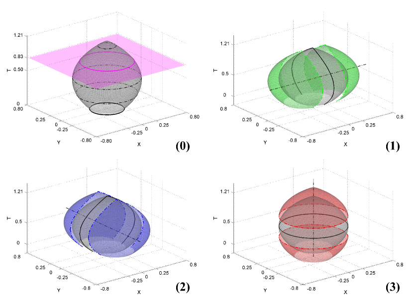
Fig. 1: Chart decomposition of $\mathcal{M}$ when $c=2$ and $r_{0}=0.25$. The circle collapses to $(0,0)$ at time $T\approx 1.21$. (0) The manifold, sliced by the plane $t=0.83$ to yield the magenta curve $\mathcal{C}_{0.83}$. Three other typical curves $\mathcal{C}_{t}$ are featured with dashed lines. $\mathcal{C}_{0}$ appears as a thick plain line. (1) $\mathcal{M}$ along with $\mathcal{W}_{1,-}$ and $\mathcal{W}_{1,+}$ appearing in green. (2) $\mathcal{M}$ along with $\mathcal{W}_{2,-}$ and $\mathcal{W}_{2,+}$ appearing in blue. (3) $\mathcal{M}$ along with $\mathcal{W}_{3,-}$ and $\mathcal{W}_{3,+}$ appearing in red.

Consider the following atlas $\mathscr{A}$ to describe the resulting $C^{0}$-manifold $\mathcal{M}$ featured on Figure 1. Let $\mathcal{U}:=\mathbb{R}\times[0,T]$. Then $\mathscr{A}=\cup^{3}_{i=1}\{(\psi_{i,\pm},\mathcal{W}_{i,\pm})\}$ where the real-valued functions $\psi_{i,\pm}$ are defined as:

$$\begin{array}[]{ll}\psi_{1,-}:\mathcal{U}\longrightarrow[-R,0]&\qquad\psi_{1,+}:\mathcal{U}\longrightarrow[0,R]\\ \psi_{2,-}:\mathcal{U}\longrightarrow[-R,0]&\qquad\psi_{2,+}:\mathcal{U}\longrightarrow[0,R]\\ \psi_{3,-}:\mathbb{R}^{2}\longrightarrow[0,\frac{1}{c})&\qquad\psi_{3,+}:\mathbb{R}^{2}\longrightarrow(\frac{1}{c},T]\end{array}$$ (11)

and

$$\psi_{1,\pm}(y,t) = \pm\sqrt{\left(r_{0}-c\,t^{2}/2+t\right)^{2}-y^{2}}$$ (12)

$$\psi_{2,\pm}(x,t) = \pm\sqrt{\left(r_{0}-c\,t^{2}/2+t\right)^{2}-x^{2}}$$ (13)

$$\psi_{3,\pm}(x,y) = \frac{1}{c}\left(1\pm\sqrt{1-2c(r(\vec{\mathbf{x}})-r_{0})}\right)$$ (14)

We also define the sets $\mathcal{W}_{i,\pm}$ as the real part of the image of the functions $\psi_{i,\pm}$. Those sets are featured on Figure 1. The functions $\psi_{3,\pm}$ can be verified to be the unique classical solutions to:

$$\left\{\begin{array}[]{rcll}|\nabla\psi_{3,-}(\vec{\mathbf{x}})|&=&\frac{1}{F(\psi_{3,-}(\vec{\mathbf{x}}))}&\quad\mathrm{on}~{}\mathcal{U}_{3,-}\\ \psi_{3,-}(\vec{\mathbf{x}})&=&0&\quad\mathrm{on}~{}\mathcal{C}_{0}\end{array}\right.$$ (17)

$$\left\{\begin{array}[]{rcll}|\nabla\psi_{3,+}(\vec{\mathbf{x}})|&=&-\frac{1}{F(\psi_{3,+}(\vec{\mathbf{x}}))}&\quad\mathrm{on}~{}\mathcal{U}_{3,+}\\ \psi_{3,+}(\vec{\mathbf{x}})&=&\frac{1}{c}&\quad\mathrm{on}~{}\mathcal{C}_{1/c}\end{array}\right.$$ (20)

where $\mathcal{U}_{3,-}=\{\vec{\mathbf{x}}:r_{0}<r(\vec{\mathbf{x}})<R\}$ and $\mathcal{U}_{3,+}=\{\vec{\mathbf{x}}:0\leq r(\vec{\mathbf{x}})<R\}$. Together, the graphs of $\psi_{3,-}$ and $\psi_{3,+}$ describe all of $\mathcal{M}$ but the circle of radius $R$ reached at time $t=\frac{1}{c}$. On the other hand this circle lies in the union of the images of $\psi_{1,\pm}$ and $\psi_{2,\pm}$. Those functions are the unique classical solutions to

$$\left\{\begin{array}[]{cl}\mp(\psi_{1,\pm})_{t}+F(t)\sqrt{1+(\psi_{1,\pm})^{2}_{y}}=0&~{}\mathrm{on}~{}\mathbb{R}\times(0,T]\\ \psi_{1,\pm}(y,0)=\pm\sqrt{r^{2}_{0}-y^{2}}&~{}\mathrm{on}~{}\mathbb{R}\times\{0\}\end{array}\right.$$ (23)

$$\left\{\begin{array}[]{cl}\mp(\psi_{2,\pm})_{t}+F(t)\sqrt{(\psi_{2,\pm})^{2}_{x}+1}=0&~{}\mathrm{on}~{}\mathbb{R}\times(0,T]\\ \psi_{2,\pm}(x,0)=\pm\sqrt{r^{2}_{0}-x^{2}}&~{}\mathrm{on}~{}\mathbb{R}\times\{0\}\end{array}\right.$$ (26)

This suggests the following procedure to build $\mathcal{M}$: (1) First, solve for $\psi_{3,-}$. (Inter.) Then solve for $\psi_{1,\pm}$ and $\psi_{2,\pm}$ restricted to $[-R,R]\times[\frac{1}{c}-\epsilon,\frac{1}{c}+\epsilon]$ for some $\epsilon>0$. (2) Finally, solve for $\psi_{3,+}$.

Some questions immediately come to mind. Criteria to decide when to move from (1) to the intermediate step must be chosen. Similarly, knowing which equation to solve within the intermediate step is a concern. The practical aspects of how a code reconciles the results of those steps need to be addressed carefully. We discuss all of these issues, and, as a result, turn the above formal idea into an efficient algorithm that constructs $\mathcal{M}$.

2.5 Notation

To lighten the notation, we will now work in the setting where $n=2$. All the results discussed extend to arbitrary $n$.

Continuous setting

We use the letter $\psi$ to denote functions whose image locally describes $\mathcal{M}$. Suppose $\psi:\mathcal{U}\mapsto\mathbb{R}$ with $\psi:(y,t)\mapsto\psi(y,t)=x$. We introduce the following subsets of $\mathbb{R}^{2}$:

$$\Gamma_{t} := \{(x,y)\in\mathbb{R}^{2}:\psi(y,t)=x,(y,t)\in\mathcal{U}\}$$ (27)

See Figure 2 for an illustration. We distinguish between $\hat{\mathfrak{n}}(\vec{\mathbf{x}},t)$ the two-dimensional outward normal to $\mathcal{C}_{t}$ at $\vec{\mathbf{x}}$; and $\hat{n}(\vec{\mathbf{x}},t)$ the three-dimensional outward normal to $\mathcal{M}$ at $(\vec{\mathbf{x}},t)$.

Discrete setting

The spatial grids have fixed meshsize $\Delta x=\Delta y=:h$. We use

$$x_{i}=i\cdot h\quad y_{j}=j\cdot h\quad t^{k}=k\cdot\Delta t\qquad(i,j,k)\in\mathbb{Z}\times\mathbb{Z}\times\{\mathbb{N}\cup\{0\}\}$$ (28)

to denote discrete values of space and time. We usually make no distinction between the continuous functions $\psi$ and their discrete approximations, except in §4. We will be using indices consistently, so that $\psi_{ij}$ can be understood as $\psi(x_{i},y_{j})$ and $\psi^{k}_{i}$ as $\psi(x_{i},t^{k})$. Nevertheless, we will explicitly mention which representation is used. If a point $p$ belongs to $\mathcal{M}$, then it may be described by one or more of the following three expressions:

$$p^{k}_{j}=(\psi^{k}_{j},y_{j},t^{k})\qquad p^{k}_{i}=(x_{i},\psi^{k}_{i},t^{k})\qquad p_{ij}=(x_{i},y_{j},\psi_{ij})$$ (29)

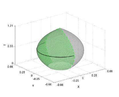
Fig. 2: The subset $\Gamma_{0.55}$ associated with $\psi_{1,-}$ from §2.4 appears as a black plain line.

3 A FMM for time-dependent speeds: The $t$-FMM

We first address the problem stated in §2.1 under the following restriction:

$$F=F(\vec{\mathbf{x}},t)\geq\delta>0\qquad\quad\forall~{}(\vec{\mathbf{x}},t)\in\mathbb{R}^{2}\times[0,T]$$ (30)

Allowing the speed to depend on time yields a non-autonomous control problem. In [55], the author studies this min-time-from-the-boundary problem in the context of anisotropic front propagation. In our context, the main result of [55] may be formulated as follows: The value function $\psi$ for this control problem satisfies the following Hamilton-Jacobi-Bellman equation:

$$H(\nabla\psi,\psi,\vec{\mathbf{x}}):=||\nabla\psi(\vec{\mathbf{x}})||F\left(\vec{\mathbf{x}},\psi(\vec{\mathbf{x}})\right)=1$$ (31)

The implementation of the resulting boundary-value problem:

$$\left\{\begin{array}[]{rcll}||\nabla\psi(\vec{\mathbf{x}})||&=&\frac{1}{F\left(\vec{\mathbf{x}},\psi(\vec{\mathbf{x}})\right)}\leq\frac{1}{\delta}&\qquad\mathrm{on}~{}\mathcal{A}^{c}_{0}\setminus\mathcal{C}_{0}\\ \psi(\vec{\mathbf{x}})&=&0&\qquad\mathrm{on}~{}\mathcal{C}_{0}\end{array}\right.$$ (34)

closely mimicks that of the classical FMM. The only step that requires modifications is the one where a tentative value is assigned to each point in the Narrow Band. Following [55] this step is adjusted as follows. Let $\vec{\mathbf{x}}_{ij}=(x_{i},y_{j})$. Without loss of generality, assume that $\vec{\mathbf{x}}_{i-1,j}$ and $\vec{\mathbf{x}}_{i,j+1}$ are Accepted neighbours of $\vec{\mathbf{x}}_{ij}$. Consider a straight line lying in Quadrant II and ending at $\vec{\mathbf{x}}_{ij}$, and suppose it intersects the line joining $\vec{\mathbf{x}}_{i-1,j}$ and $\vec{\mathbf{x}}_{i,j+1}$ at the point $\tilde{\mathbf{x}}$. See Figure 3. Then: $\tilde{\mathbf{x}}=\xi\vec{\mathbf{x}}_{i-1,j}+(1-\xi)\vec{\mathbf{x}}_{i,j+1}$ for some $\xi\in[0,1]$. Letting $\vec{v}=\vec{\mathbf{x}}_{ij}-\tilde{\mathbf{x}}$, we get $|\vec{v}|=\sqrt{\xi^{2}+(1-\xi)^{2}}~{}h$. Associate the following value to Quadrant II:

$$\psi_{\mathrm{II}}=\min_{\xi\in[0,1]}\left\{\psi(\tilde{\mathbf{x}})+\sqrt{\xi^{2}+(1-\xi)^{2}}~{}\frac{~{}h}{F(\vec{\mathbf{x}}_{ij},\psi(\tilde{\mathbf{x}}))}\right\}$$ (35)

Proceeding similarly in the other quadrants yields the values $\psi_{\mathrm{I}}$, $\psi_{\mathrm{III}}$ and $\psi_{\mathrm{IV}}$. The tentative value assigned to $\psi_{ij}$ is then $\psi_{ij}=\min\{\psi_{\mathrm{I}},~{}\psi_{\mathrm{II}},~{}\psi_{\mathrm{III}},~{}\psi_{\mathrm{IV}}\}$. Note that in two dimensions the minimization problem (35) may be solved using a direct method; see Appendix A. This method converges to the correct viscosity solution, and is globally $1^{\mathrm{st}}$ order [43, 46, 55]. Its complexity is $\mathcal{O}(N^{n}\log N^{n})$. In subsequent sections of this paper, we will refer to this modified FMM as the ‘$t$-FMM’. The results presented in this section yield Algorithm 2 given in §6. Finally, in the general case $|F|\geq\delta>0$, the PDE we wish to solve is $||\nabla\psi(\vec{\mathbf{x}})||\,|F\left(\vec{\mathbf{x}},\psi(\vec{\mathbf{x}})\right)|=1$.

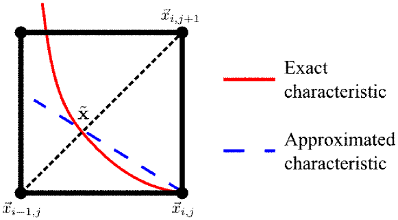
Fig. 3: If the characteristic comes from Quadrant II.

4 A local description of the evolving front: The sideways representation

An option to study the evolution of propagating curves or surfaces is to represent the front as a function that depends on time, e.g., $y=Y(x,t)$ [42]. Although successful at describing the evolution locally, this approach fails to capture the global properties of the front. Nevertheless we believe that this approach can be used near regions where $F$ vanishes.

4.1 Heuristics

We first present an argument in the smooth setting. Consider the solution $\phi$ to IVP (4). Suppose $\phi\in C^{1}(\vec{\mathbf{x}}_{0},t_{0})$ and $\phi(\vec{\mathbf{x}}_{0},t_{0})=0$. Assume furthermore that $\phi_{x}(\vec{\mathbf{x}}_{0},t_{0})\neq 0$, so that the mapping is locally invertible. From the Implicit Function Theorem there exist open neighbourhoods $(\vec{\mathbf{x}}_{0},t_{0})\in\mathcal{V}$ and $\mathcal{U}\subset\mathbb{R}\times[0,T]$, as well as a function

$$\psi:\mathcal{U}\longrightarrow\mathbb{R}~{},\quad\psi:(y,t)\mapsto x=\psi(y,t)~{},\quad\psi\in C^{1}(\mathcal{U})~{},\quad(\psi(y,t),y,t)\in\mathcal{V}$$ (36)

satisfying $\phi(\psi(y,t),y,t)=0$ $\forall~{}(y,t)\in\mathcal{U}$. Taking full derivatives of $\phi$ with respect to $y$ and $t$, and using the fact that in $\mathcal{V}$, $\phi$ satisfies the LSE pointwise gives:

$$(-\phi_{x}\psi_{t})+F\sqrt{\phi^{2}_{x}+(-\phi_{x}\psi_{y})^{2}}=0\quad\Longleftrightarrow\quad-\psi_{t}\pm F\sqrt{1+\psi^{2}_{y}}=0$$ (37)

where $\phi_{x}$ and $F$ are evaluated at $(x,y,t)=(\psi(y,t),y,t)$. The sign used in the last equation depends on $\phi_{x}=\pm\sqrt{\phi^{2}_{x}}$. We let $a:=-\mathrm{sign}(\phi_{x}(\vec{\mathbf{x}}_{0},t_{0}))$.

Now, let $\psi$ satisfy the following Initial Value Problem:

$$\left\{\begin{array}[]{cl}\psi_{t}+aF(\psi,y,t)\sqrt{1+\psi^{2}_{y}}=0&~{}\mathrm{on}~{}\mathcal{U}\cap\left(\mathbb{R}\times(t_{0},T)\right)\\ \psi(y,t_{0})=\psi_{0}(y)&~{}\mathrm{on}~{}\mathcal{U}\cap\left(\mathbb{R}\times\{t_{0}\}\right)\end{array}\right.$$ (40)

where $\psi_{0}$ is chosen such that $\phi(\psi_{0}(y),y,t_{0})=0$. Then for all $t\in(t_{0},T)$ the set $\Gamma_{t}$ locally describes the curve at time $t$, i.e., $\Gamma_{t}=\mathcal{C}_{t}\cap\mathcal{V}$. We now investigate the case where $\mathcal{M}$ is merely $C^{0}$. For simplicity, we work with $t_{0}=0$.

Remark

Applying the same argument assuming $\phi_{t}(\vec{\mathbf{x}}_{0},t_{0})\neq 0$ allows one to formally relate the LSE to the Eikonal equation [35]:

$$\phi_{t}+F(x,y,\psi)\sqrt{(-\phi_{t}\psi_{x})^{2}+(-\phi_{t}\psi_{y})^{2}}=0\quad\Longleftrightarrow\quad||\nabla\psi||=\frac{-\mathrm{sign}({\phi}_{t})}{F(x,y,\psi)}$$ (41)

But since by the LSE we have $a:=-\mathrm{sign}(\phi_{t})=\mathrm{sign}\left(F(x,y,\psi)\right)$, this simplifies to $||\nabla\psi||=\frac{1}{|F(x,y,\psi)|}$.

4.2 Theory

Equation (40) is a Cauchy problem of the form

$$\left\{\begin{array}[]{cl}\psi_{t}+H(y,t,\psi,\psi_{y})=0&~{}\mathrm{on}~{}\mathcal{U}\cap\left(\mathbb{R}\times(0,T)\right)\\ \psi(y,0)=\psi_{0}(y)&~{}\mathrm{on}~{}\mathcal{U}\cap\left(\mathbb{R}\times\{0\}\right)\end{array}\right.$$ (44)

where the Hamiltonian $H:\mathbb{R}^{1}\times(0,T)\times\mathbb{R}\times\mathbb{R}^{1}\rightarrow\mathbb{R}$ is defined as $H(y,t,\psi,\psi_{y})=aF(\psi,y,t)\sqrt{1+\psi^{2}_{y}}$. The function $\psi_{0}$ is defined such that for all $y\in\mathcal{U}\cap\left(\mathbb{R}\times\{0\}\right)$ we have $(\psi_{0}(y),y)\in\mathcal{C}_{0}$. We resort to the rich theory of viscosity solutions of Hamilton-Jacobi equations to study various properties of this problem [7, 8, 14, 15, 17, 24, 28, 49, 50]. We first address the well-posedness of the PDE. It is a simple matter to verify that the assumptions on $H$ required to apply Theorem 1.1 in [48] hold in our context. This yields

Theorem 1 (Existence & Uniqueness).

There exists a unique viscosity solution $\psi$ to problem (44).

We next verify that (44) does have the geometric interpretation advertised in the previous section.

Theorem 2 ($\Gamma_{t}$ locally describes $\mathcal{C}_{t}$).

The set $\Gamma_{t}$ enjoys the following property: $\Gamma_{t}=\mathcal{C}_{t}\cap\mathcal{V}$.

Proof.

Consider IVP (4) again:

$$\left\{\begin{array}[]{rcll}\phi_{t}+F|\nabla\phi|&=&0&\quad\mathrm{on}~{}\mathbb{R}^{2}\times(0,T)\\ \phi(\vec{\mathbf{x}},0)&=&\phi_{0}(\vec{\mathbf{x}})&\quad\mathrm{on}~{}\mathbb{R}^{2}\times\{0\}\end{array}\right.$$ (47)

Since it is known that $\vec{\mathbf{x}}\in\mathcal{C}_{t}\cap\mathcal{V}$ if and only if $\phi(\vec{\mathbf{x}},t)=0$, we may prove the theorem by showing that: $\vec{\mathbf{x}}\in\Gamma_{t}$ if and only if $\phi(\vec{\mathbf{x}},t)=0$.

$\Longrightarrow$ We argue by contradiction. Suppose the set $\mathcal{T}=\{T>t>0:\exists\vec{\mathbf{x}}\in\Gamma_{t}\mathrm{~{}s.t.~{}}\phi(\vec{\mathbf{x}},t)\neq 0\}$ is not empty and define $t^{\ast}=\inf\mathcal{T}$. Since $\phi$ is continuous, $\mathcal{T}$ is open and $t^{\ast}\not\in\mathcal{T}$. Therefore, for all $\vec{\mathbf{x}}^{\ast}\in\Gamma_{t^{\ast}}$, $\phi(\vec{\mathbf{x}}^{\ast},t^{\ast})=0$, but for any $\epsilon>0$ sufficiently small, there exists $\vec{\mathbf{x}}_{\epsilon}\in\Gamma_{t+\epsilon}$ such that $\phi(\vec{\mathbf{x}}_{\epsilon},t+\epsilon)\neq 0$. If $\mathcal{M}$ is differentiable at $(\vec{\mathbf{x}}^{\ast},t^{\ast})$, this contradicts the argument presented in §4.1: The Implicit Function Theorem guarantees that the set $\mathcal{V}$ is open. If $\mathcal{M}$ is not differentiable at $(\vec{\mathbf{x}}^{\ast},t^{\ast})$, then fix $\epsilon$ and for $\delta>0$ consider $\vec{\mathbf{x}}^{0}\in\Gamma_{t+\epsilon}$ such that $\|\vec{\mathbf{x}}_{\epsilon}-\vec{\mathbf{x}}^{0}\|\leq\delta$ and $\mathcal{M}$ is differentiable at $(\vec{\mathbf{x}}^{0},t+\epsilon)$. For any $\delta$, such a point can be found since for any $T>t+\epsilon>0$ the singularities of $\Gamma_{t+\epsilon}$ are subsets of measure 0. Again, the Implicit Function Theorem guarantees that there is a neighbourhood $\tilde{\mathcal{V}}$ of $(\vec{\mathbf{x}}^{0},t+\epsilon)$ where $\phi(\vec{\mathbf{x}},t)=0$ for any $\vec{\mathbf{x}}\in\Gamma_{t}\cap\tilde{\mathcal{V}}$. Considering the sequence $\delta_{n}=\{\frac{1}{n}:n\in\mathbb{N}\}$ and the corresponding sequence $\{\vec{\mathbf{x}}^{n}\}^{\infty}_{n=1}$, we arrive at the conclusion that $\phi(\vec{\mathbf{x}}_{\epsilon},t+\epsilon)\neq 0$ contradicts the continuity of $\phi$.

$\Longleftarrow$ Assume that there exists $(\vec{\mathbf{x}},t)\in\mathcal{V}$ such that $\phi(\vec{\mathbf{x}},t)=0$, but there is no $y$ such that $\vec{\mathbf{x}}=(\psi(y),y)\in\Gamma_{t}$. We re-use the arguments given in the proof of $\Longrightarrow$: If $\mathcal{M}$ is differentiable at $(\vec{\mathbf{x}},t)$ then this contradicts the argument in §4.1. If $\mathcal{M}$ is not differentiable at $(\vec{\mathbf{x}},t)$, then we can find a sequence $\vec{\mathbf{x}}^{n}\in\Gamma_{t}$ converging to $\vec{\mathbf{x}}$ such that $\phi(\vec{\mathbf{x}}^{n},t)=0$, and obtain the contradiction that $\psi$ is not continuous.   ∎

4.3 Generalizations

More generally, the above arguments can be applied to yield that there exists neighbourhoods $(\vec{\mathbf{x}}_{0},t_{0})\in\mathcal{V}$ and $\mathcal{U}\subset\mathbb{R}\times[0,T]$, as well as a unique function $\psi:\mathcal{U}\longrightarrow\mathbb{R}$, $\psi:(z,t)\mapsto w=\psi(z,t)$ with $(w\cos(\theta)+z,w\sin(\theta)+z,t)\in\mathcal{V}$ satisfying

$$\left\{\begin{array}[]{cl}\psi_{t}+aF\left(w\cos(\theta)+z,w\sin(\theta)+z,t\right)\sqrt{\psi^{2}_{z}+1}=0&~{}\mathrm{on}~{}\mathcal{U}\cap\left(\mathbb{R}\times(0,T)\right)\\ \psi(z,0)=\psi_{0}(z)&~{}\mathrm{on}~{}\mathcal{U}\cap\left(\mathbb{R}\times\{0\}\right)\end{array}\right.$$ (50)

in the viscosity sense. Here $\theta$ is the polar angle of $\vec{\mathbf{x}}_{0}$, $a=-\mathrm{sign}(\vec{\mathbf{x}}_{0}\cdot\hat{\mathfrak{n}}(\vec{\mathbf{x}}_{0},t_{0}))$ and $\psi_{0}$ is chosen such that for all $z\in\mathcal{U}\cap\left(\mathbb{R}\times\{0\}\right)$, we have $(\psi_{0}(z)\cos(\theta)+z,\psi_{0}(z)\sin(\theta)+z)\in\mathcal{C}_{0}$. When $\theta=0$ we recover Problem (40), whereas when $\theta=\pi/2$, we get that $\psi:(x,t)\mapsto y=\psi(x,t)$ with $(x,\psi(x,t),t)\in\mathcal{V}$ satisfies:

$$\left\{\begin{array}[]{cl}\psi_{t}+aF(x,\psi,t)\sqrt{\psi^{2}_{x}+1}=0&~{}\mathrm{on}~{}\mathcal{U}\cap\left(\mathbb{R}\times(0,T)\right)\\ \psi(x,0)=\psi_{0}(x)&~{}\mathrm{on}~{}\mathcal{U}\cap\left(\mathbb{R}\times\{0\}\right)\end{array}\right.$$ (53)

in the viscosity sense. In subsequent sections, we will refer to Problems (40) and (53) as the $yt$- and $xt$-representations of $\mathcal{M}$, whereas Problem (50) will be the skewed representation. Those problems provide sideways representations of the evolving front. For clarity, remarks pertaining to those will usually be made for the special case of Problem (40).

4.4 Discretization

Finite-differences schemes for problems such as (44) have been discussed [16, 18, 48]. Based on these works, we propose the following discretization for Equation (40). In this subsection only, we will distinguish between the continuous function $\psi$, and its discrete approximation which we denote as $\chi$. The spatial derivative $\chi_{y}$ must be computed in an upwind fashion. To this end, we introduce the one-sided operators

$$D^{+}_{l}\chi^{r}:=\frac{\chi^{r}_{l+1}-\chi^{r}_{l}}{h}\qquad\qquad D^{-}_{l}\chi^{r}:=\frac{\chi^{r}_{l}-\chi^{r}_{l-1}}{h}$$ (54)

and suggest:

$$\chi^{r+1}_{l}=\chi^{r}_{l}-a\cdot\Delta t\cdot F(\chi^{r}_{l},y_{l},t^{r})\cdot\sqrt{1+\mathrm{upw}(\chi^{r},l,r,\alpha)}$$ (55)

where

$$\mathrm{upw}(\chi^{r},l,n,\alpha) := \max\{\alpha,0\}\left(\min\left\{D^{+}_{l}\chi^{r},0\right\}^{2}+\max\left\{D^{-}_{l}\chi^{r},0\right\}^{2}\right)$$ (56)

$$-\min\{0,\alpha\}\left(\max\left\{D^{+}_{l}\chi^{r},0\right\}^{2}+\min\left\{D^{-}_{l}\chi^{r},0\right\}^{2}\right)$$

The constant $\alpha$ acts as a switch and is defined as $\alpha=\mathrm{sign}\left(aF(\chi^{r}_{l},y_{l},t^{r})\right)$.

Proposition 3.

(Convergence.) Let $M$ be defined as the local bound on $F$, i.e., $M^{r}_{l}=\sup_{(x,y,t)\in B(p^{r}_{l},2h)}\{|F(x,y,t)|\}$, where $p^{r}_{l}=(\chi^{r}_{l},y_{l},t^{r})$. Assume that $\max\left\{|D^{+}_{l}\chi^{r}|,|D^{-}_{l}\chi^{r}|\right\}\leq P$ for all $l\in L$ and $0\leq r\leq R$. Suppose $\Delta t$ satisfies

$$M^{r}_{l}\cdot\Delta t\leq\frac{h}{2P}$$ (57)

Then the above scheme is such that $\chi\rightarrow\psi$ as $h$ and $\Delta t\rightarrow 0$, with rate

$$\|\chi-\psi\|_{\infty}\leq c\sqrt{\Delta t}$$ (58)

for all $l$, where the constant $c$ depends on $\|\psi_{0}\|$, $\|D\psi_{0}\|$, the numerical Hamiltonian $g$, and $R\Delta t$ where $0\leq r\leq R$.

Proof.

We proceed by showing that the scheme is monotone and consistent in the sense of [48]. The results then follow from Theorem 3.1 of that same paper. The scheme can be rewritten as

$$\chi^{r+1}_{l}=\chi^{r}_{l}-\Delta t\cdot g\left(y_{l},t^{r},\chi^{r}_{l},D^{+}_{l}\chi^{r},D^{-}_{l}\chi^{r}\right)$$ (59)

where the numerical Hamiltonian $g$ is easily verified to be consistent, i.e.,

$$g\left(y,t,s,\delta,\delta\right)=H(y,t,s,\delta)\qquad\forall(y,t)\in\mathcal{U},~{}s\in\mathbb{R},~{}|\delta|<P$$ (60)

We verify monotonicity by showing that the function

$$G(\chi^{r}_{l-1},\chi^{r}_{l},\chi^{r}_{l+1})=\chi^{r}_{l}-a\cdot\Delta t\cdot F(u,y_{l},t^{r})\cdot\sqrt{1+\mathrm{upw}(\chi^{r},l,r,\alpha)}$$ (61)

is a non-decreasing function of each of its argument, for fixed $u$, $y_{l}$ and $t^{r}$. We only treat the case $\alpha>0$, since the other case is symmetric. Writing $F=F(u,y_{l},t^{r})$ for short gives

$$G(b,c,d)=\left\{\begin{array}[]{ll}c-a\Delta t~{}F\sqrt{1+\left(\frac{d-c}{h}\right)^{2}}&\mathrm{if}~{}d-c<0,~{}c-b<0\\ c-a\Delta t~{}F\sqrt{1+\left(\frac{c-b}{h}\right)^{2}}&\mathrm{if}~{}d-c>0,~{}c-b>0\\ c-a\Delta t~{}F\sqrt{1+\left(\frac{d-c}{h}\right)^{2}+\left(\frac{c-b}{h}\right)^{2}}&\mathrm{if}~{}d-c<0,~{}c-b>0\\ c-a\Delta t~{}F&\mathrm{if}~{}d-c>0,~{}c-b<0\end{array}\right.$$ (66)

For the first case: $G_{b}$, $G_{d}\geq 0$ are trivial to check while $G_{c}\geq 0$ only if

$$1\geq\left(F^{2}\left(\frac{\Delta t}{h}\right)^{2}-1\right)\left(-\frac{d-c}{h}\right)^{2}\quad\Longleftarrow\quad\frac{\sqrt{1+P^{2}}}{P}\geq M^{r}_{l}\frac{\Delta t}{h}$$ (67)

Case 2 yields the same condition, whereas Case 3 gives the more restrictive one present in the assumption of the claim. Case 4 is trivial.   ∎

Proposition 4.

(Stability.) The above scheme is stable, provided that

$$\Delta t<\min\left\{\frac{h}{2PM^{r}_{l}}~{},~{}\frac{P-2}{KP\sqrt{1+2P^{2}}}~{},~{}\frac{2}{P\delta}\right\}$$ (68)

for some $\delta>0$. The constant $P$ is such that $\max\left\{|D^{+}_{l}\chi^{r}|,|D^{-}_{l}\chi^{r}|\right\}\leq P$ for all $l\in L$ and $0\leq r\leq R$.

Proof.

Applying Theorem 7 of [34] to our scheme, it is possible to show that for $h$ small enough, the explicit Euler map defined as

$$S^{l}_{\Delta t}(\chi)=\chi_{l}-a\Delta t\cdot F(\chi_{l},y_{l},t)\sqrt{1+\mathrm{upw}(\chi^{r},l,r,\alpha)}$$ (69)

is a strict contraction in $\ell_{\infty}$. Bounding $S^{l}_{\Delta t}(\chi)-S^{l}_{\Delta t}(\tau)$ from below (resp. above) yields the $2^{\mathrm{nd}}$ (resp. $3^{\mathrm{rd}}$) bound in (68). ∎

When defining ‘upw’, we implicitly assumed that both $\chi^{r}_{l+1}$ and $\chi^{r}_{l-1}$ were known. In the instance where one of those values is not known, we set $\chi^{r+1}_{l}$ to $+\infty$. Indeed, no value can be assigned to $\chi^{r+1}_{l}$ since it is not possible to infer where the characteristic going through the point $p^{r}_{l}=(\chi^{r}_{l},y_{l},t^{r})$ comes from.

Remark

Assuming $P=\mathcal{O}(1/h)$, we may revisit the bounds on $\Delta t$ given in (68). The first bound is not very restrictive, even though it scales like $\mathcal{O}(h^{2})$. Indeed $F\approx 0$ implies that $M^{r}_{l}$ should always be small. The bounds imposed by stability are $\mathcal{O}(h)$, which agrees with the usual CFL number of an advection problem.

5 Weaving the representations

Both approaches just discussed in §3 and §4 provide methods that locally build the manifold $\mathcal{M}$. We now address the question of when to use a specific representation.

5.1 The Sign Test

Since the approach presented in §3 relies on the assumption that the speed is bounded away from 0, the sign of $F$ is monitored throughout the algorithm. In particular, whenever a point in $(x_{i},y_{j})$ is assigned a value $\psi_{ij}$ using the $(t)$-FMM, the Sign Test is performed as follows. Suppose the point $p_{i-1,j}=(x_{i-1},y_{j},\psi_{i-1,j})$ was used in the computation of $\psi_{ij}$. Considering the line in $xyt$-space joining the point $p_{i-1,j}$ and $p_{ij}$, we check the number of times $d$ that the speed changes sign along this line. If $d=0$, the algorithm can keep running the ($t$-)FMM: The pair $(p_{i-1,j},p_{ij})$ is said to pass the Sign Test. If $d=1$, we should change representation: The pair $(p_{i-1,j},p_{ij})$ fails the Sign Test. If $d>1$, the grid has to be refined.

5.2 Conversion of data: Interpolation

Suppose that the pair $(p_{i-1,j},p_{ij})$ just failed the Sign Test discussed in §5.1. Then the algorithm must change representation. Without loss of generality, let us suppose that the algorithm switches from the $xy$- to the $yt$-representation. This means the manifold is locally sampled by points of the form $p_{lm}=(x_{l},y_{m},t)$, where $l\in L\subset I$ and $m\in M\subset J$. The $yt$-representation requires points of the form $p^{r}_{m}=(x,y_{m},t^{r})$, where $r\in R\subset K$. See Figure 4.

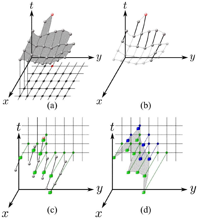
Fig. 4: Converting the data using interpolation. (a) Some data in the $xy$-representation. The point $p_{\alpha\beta}$ appears in red. (b) We only keep those points used for interpolation. (c) Performing one-dimensional interpolation line by line, we obtain data in the $yt$-representation. Those are the light green squares. (d) Using the boundary data from (c), the sideways PDE can be solved, to obtain the dark blue squares. By design, the domain shrinks by two points every time step.

5.3 Computing the outward normal

Computing the outward normal $\hat{n}$ accurately at each point sampling $\mathcal{M}$ is a crucial component of the algorithm. In regions where the level-set function $\phi$ is $C^{1}$, we have $\hat{n}=\frac{(\phi_{x},\phi_{y},\phi_{t})}{|(\phi_{x},\phi_{y},\phi_{t})|}$. We use the Implicit Function Theorem: If $\psi(y,t)=x$ satisfies $\phi(\psi(y,t),y,t)=0$, then $\phi_{y}=-\phi_{x}\psi_{y}$ and $\phi_{t}=-\phi_{x}\psi_{t}$. Since $\phi_{x}\neq 0$, we set $\vec{n}=(+\mathrm{sign}(\phi_{x}),\psi_{y},\psi_{t})$ and $\hat{n}=\vec{n}/|\vec{n}|$. We keep track of the normal associated to each point by defining the function

$$\mathrm{\textsl{Norm}~{}}:\mathbb{R}^{2}\times\mathbb{R}^{+}\longrightarrow S^{2}\qquad\qquad\mathrm{\textsl{Norm}~{}}(p_{ij})=\hat{n}(p_{ij})$$ (70)

5.4 The Orientation Test

Whenever a point is computed, the algorithm determines the orientation of the outward normal at this point. As explained in §4, this can be done based on the sign of $\hat{n}_{3}$, the time component of $\hat{n}$. We define

$$\mathrm{\textsl{Orient}3~{}}:\mathbb{R}^{2}\times\mathbb{R}^{+}\longrightarrow\{-1,+1\}\qquad\qquad\mathrm{\textsl{Orient}3~{}}(p_{ij})=-\mathrm{sign}\left(\hat{n}_{3}\right)$$ (71)

The algorithm requires finding which points $p_{ab}$ in a neighbourhood of $p_{ij}$ have the same orientation as $p_{ij}$. This is done using the Orientation Test. A pair $(p_{ij},p_{ab})$ is said to pass the Orientation Test if $\mathrm{\textsl{Orient}3~{}}(p_{ij})=\mathrm{\textsl{Orient}3~{}}(p_{ab})$, and to fail it otherwise.

6 Algorithms & Discussion

We introduce some notation before giving the details of the algorithms. We make use of four lists. Accepted and Narrow Band are lists of triplets, e.g., $p_{ij}=(x_{i},y_{j},\psi_{ij})$. Pile and Far Away are lists of coordinates, e.g., $(x_{i},y_{j})$. We define the space and time projection operators as follows: if $p_{ij}=(x_{i},y_{j},\psi_{ij})$, then

$$\pi_{s}:\mathbb{R}^{2}\times\mathbb{R}^{+}\longrightarrow\mathbb{R}^{2} \pi_{s}(p_{ij})=(x_{i},y_{j})$$ (72)

$$\pi_{t}:\mathbb{R}^{2}\times\mathbb{R}^{+}\longrightarrow\mathbb{R}^{+} \pi_{t}(p_{ij})=\psi_{ij}$$ (73)

The following function will be used:

$$\mathrm{\textsl{Grid}}:\mathbb{R}^{2}\longrightarrow\mathbb{R}^{+}\qquad\mathrm{\textsl{Grid}}:(x_{i},y_{j})\longrightarrow\psi_{ij}$$ (74)

The set of coordinates $N((x_{i},y_{j}))=\{(x_{a},y_{b}):|(i,j)-(a,b)|=1\}$ consists of the nearest neighbours of $(x_{i},y_{j})$. We use Table 1 to define two sets of triplets: $\mathrm{NeighEik}((x_{i},y_{j}))$ and $\mathrm{NeighSide}(p_{\alpha\beta})$. The first one is used to compute the value $\psi_{ij}$ in Algorithms 5 and 2. Similarly the second set is used in Algorithm 4, where the relevant component of $\hat{n}(p_{\alpha\beta})$, the normal at $p_{\alpha\beta}$, is denoted by $\eta_{i}$. We are now ready to present the main algorithms.

	$\mathcal{S}=\mathrm{NeighEik}((x_{i},y_{j}))$	$\mathcal{S}=\mathrm{NeighSide}(p_{\alpha\beta})$
$p_{ab}=(x_{a},y_{b},\psi_{ab})$	• $(x_{a},y_{b})\in N((x_{i},y_{j}))$	• $(x_{a},y_{b})\in\{(x_{l},y_{m}):l\in L,m\in M\}$
belongs to $\mathcal{S}$	• $p_{ab}\in$ Accepted	• $p_{ab}\in$ Accepted
if it satisfies	• Grid$(x_{a},y_{b})=\psi_{ab}$	• $\mathrm{sign}(\eta_{i})=\mathrm{sign}(\hat{n}_{i})$
	• $(p_{\alpha\beta},p_{ab})$ passes the Orient.Test	where $\hat{n}=$Norm $(p_{ab})$

Table 1: Definitions of two sets used in Algorithms 2, 4 and 5

Algorithm 1 Main Loop

1:while Narrow Band$\neq\emptyset$ do

2:

3:     procedure Accept a point

4:         $\psi_{\alpha\beta}\leftarrow\min\{\pi_{t}(p_{ij}):p_{ij}\in$ Narrow Band$\}$

5:         Grid$(x_{\alpha},y_{\beta})\leftarrow\psi_{\alpha\beta}$,   $p_{\alpha\beta}\leftarrow(x_{\alpha},y_{\beta},\psi_{\alpha\beta})$

6:         remove $p_{\alpha\beta}$ from Narrow Band       add $p_{\alpha\beta}$ to Accepted

7:         if $(x_{\alpha},y_{\beta})\in$ Far Away then

8:              remove $(x_{\alpha},y_{\beta})$ from Far Away              

9:

10:     if $\psi_{\alpha\beta}<T$ then

11:         procedure Update Pile

12:              for all $(x_{a},y_{b})\in N((x_{\alpha},y_{\beta}))$ do

13:                  $\vec{v}\leftarrow(x_{a},y_{b})-(x_{\alpha},y_{\beta})$

14:                  if $\mathrm{sign}(\vec{v}\cdot\hat{\mathfrak{n}}(p_{\alpha\beta}))=\mathrm{sign}(F(p_{\alpha,\beta}))$ or 0 then

15:                       if Grid$(x_{a},y_{b})=\psi_{ab}<+\infty$ then

16:                           $p_{ab}\leftarrow(x_{a},y_{b},\psi_{ab})$

17:                           if Orient3 $(p_{ab})\neq$Orient3 $(p_{\alpha\beta})$  then

18:                                add $(x_{a},y_{b})$ to Pile                           

19:                       else if $(x_{a},y_{b})\in$ Far Away then

20:                           add $(x_{a},y_{b})$ to Pile                                                                     

21:

22:     procedure Update the Narrow Band

23:         for all $(x_{i},y_{j})\in$ Pile do

24:              compute $\psi_{ij}$ and $\hat{n}_{ij}$ using Algo. 5 if $F=F(\vec{\mathbf{x}})$ or Algo. 2 if $F=F(\vec{\mathbf{x}},t)$

25:              $p_{ij}\leftarrow(x_{i},y_{j},\psi_{ij})$,   Norm $(p_{ij})\leftarrow\hat{n}(p_{ij})$

26:              remove $(x_{i},y_{j})$ from Pile.

27:              for all $p\in\mathrm{NeighEik}((x_{i},y_{j}))$ do

28:                  perform the Sign Test for the pair $(p_{ij},p)$               

29:              if at least one pair fails the Sign Test then

30:                  proceed to Algo. 3, which returns $(k,l,\psi_{kl})$, FAIL and $\hat{n}$

31:                  $p_{ij}\leftarrow(x_{k},y_{l},\psi_{kl})$,   Norm $(p_{ij})\leftarrow\hat{n}$,    $i\leftarrow k$,   $j\leftarrow l$               

32:              Orient3 $(p_{ij})\leftarrow-\mathrm{sign}(\hat{n}_{3}(p_{ij}))$

33:              if FAIL$==0$ then

34:                  if $\exists~{}q_{ij}\in$ Narrow Band with $\pi_{s}(q_{ij})=\pi_{s}(p_{ij})$ then

35:                       remove $q_{ij}$ from Narrow Band                  

36:                  add $p_{ij}$ to Narrow Band                            

Algorithm 2 Solve $|\nabla\psi(x,y)|=\frac{1}{|F(x,y,\psi)|}$

$u_{\pm}\leftarrow\pi_{t}(p_{i\pm 1j})$ if $p_{i\pm 1j}\in\mathrm{NeighEik}((x_{i},y_{j}))$, $+\infty$ otherwise.

$v_{\pm}\leftarrow\pi_{t}(p_{ij\pm 1})$ if $p_{ij\pm 1}\in\mathrm{NeighEik}((x_{i},y_{j}))$, $+\infty$ otherwise.

$\Theta\leftarrow[0,0,0,0]$

for Quadrant=1…4 do

     if Quadrant=1 then

         $\psi_{v}\leftarrow v_{+}$,  $\psi_{u}\leftarrow u_{+}$,  $\tau_{v}\leftarrow\frac{h}{|F(x_{i},y_{j+1},\psi_{v})|}$,  $\tau_{u}\leftarrow\frac{h}{|F(x_{i+1},y_{j},\psi_{u})|}$,       

     (and similarly for other quadrants)

     if $(\psi_{v}=+\infty)$ and $(\psi_{u}=+\infty)$ then

         $\theta\leftarrow+\infty$,  

     else

         $\theta\leftarrow\min_{\xi\in[0,1]}\{\xi\psi_{v}+(1-\xi)\psi_{u}+\sqrt{\xi^{2}+(1-\xi)^{2}}~{}\left(\xi\tau_{v}+(1-\xi)\tau_{u}\right)\}$

         (see Appendix A for details)      

     $\Theta$(Quadrant)$\leftarrow\theta$,  

$\psi_{ij}\leftarrow\min(\Theta)$,   $Q\leftarrow\mathrm{argmin}(\Theta)$

6.1 Algorithm 1, Main loop

All steps of the main loop can be checked to be such that if $F=F(x,y)\geq\delta>0$, $\forall(x,y)\in\mathbb{R}^{2}$, it reduces to the classical FMM. The sideways formulations are only used when $F\approx 0$. The first procedure, ‘Accept a point’ is identical to the acceptance procedure in the standard FMM [41], and we therefore omit to discuss it. For clarity, the point accepted during this step is labelled as $p_{\alpha\beta}=(x_{\alpha},y_{\beta},\psi_{\alpha\beta})$ in the rest of the discussion.

6.1.1 Update Pile

This step is only performed if $\psi_{\alpha\beta}$ is below a certain predefined time $T$ to ensure that Narrow Band is eventually empty. At this stage the algorithm needs to decide whether a nearest neighbour $(x_{a},y_{b})$ of $p_{\alpha\beta}$ should be put in Pile. To this end three criteria are used: the position, status and orientation of that neighbour. Simply put, line 12 has the following effect: If $F(p_{\alpha\beta})>0$ and the considered neighbour lies inside the curve $\mathcal{C}_{\psi_{\alpha\beta}}$, then the pair $(x_{a},y_{b})$ is not added to Pile. Next the status of this nearest neighbour is considered. If the pair $(x_{a},y_{b})$ was traversed by the curve in the past, then it is only added to Pile if $p_{ab}:=(x_{a},y_{b},$Grid$(x_{a},y_{b}))$ and $p_{\alpha\beta}$ have different orientations (lines 13-16). Indeed a point in the plane can only be traversed twice if the speed has changed sign in the meantime. If $(x_{a},y_{b})$ is still in Far Away, then it is automatically added to Pile (lines 17-18).

Remark

The presence of the ‘if $\psi_{\alpha\beta}<T$’ in line 8 is in contrast with the standard FMM, where it is proved that since $F\geq\delta>0$, all characteristics exit the domain in finite time. In this context, the size of the computational domain determines $T$.

6.1.2 Update the Narrow Band

This procedure assigns tentative values to the points in Pile using either the standard FMM (see Appendix B) or Algorithm 2, depending on the domain of $F$. Since $\psi$ only solves the Eikonal equation in regions where $|F|\geq\delta>0$, the first lines of those algorithms ensure that the points involved in the computation of $\psi_{ij}$ all lie in one such region. The steps outlined in lines 24-28 represent the main modification to the standard FMM algorithm. The Sign Test is performed to check if the value returned by Algorithm 5 or 2 is valid. If it is not, then Algorithm 3 is called. Using a sideways representation, it attempts to return a point $(x_{k},y_{l},\psi_{kl})\in\mathcal{C}_{\psi_{kl}}$. If it manages to do so, note that as explained in §6.2.4, the triplet returned may not be $(x_{i},y_{j},\psi_{ij})$, which is why $i$ and $j$ are relabelled in line 28. As in the standard FMM, if there already is a point in Narrow Band with the same spatial coordinates $(x_{i},y_{j})$, then it is automatically removed from that list. The triplet $(x_{i},y_{j},\psi_{ij})$ is added to Narrow Band. In the event where Algorithm 3 fails, no new point is added to Narrow Band.

6.2 Algorithm 3, Sideways representation

This algorithm is called by the main loop when the speed $F$ is close to 0.

6.2.1 Determine representation

In order to work locally, the first step of this procedure defines a square of side length at most $2sh$ for some $s\in\mathbb{N}$ as the new computational grid. Then the representation is chosen based on the normal at $p_{\alpha\beta}$.

6.2.2 Initialization

This is the step where data are converted, as was mentioned in §5.2. The set NeighSide$(p_{\alpha\beta})$ is found; This ensures that the orientation of the points used next is compatible with the current representation. We take time to explain what we mean in line 12 in details. It is ideal to build the sideways grid in such a way that the triplet $p_{\alpha\beta}$ is represented exactly on this grid. i.e., For example, if data are being converted to the $yt$-representation, then there should be $\tilde{l}\in L$ and $\tilde{r}\in R$ such that $(y_{\tilde{l}},t^{\tilde{r}})=(y_{\beta},\psi_{\alpha\beta})$. The function $\psi_{1}:(y,t)\mapsto x$ then satisfies $\psi_{1}(y_{\tilde{l}},t^{\tilde{r}})=x_{\alpha}$, and $(x_{\alpha},y_{\beta},\psi_{\alpha\beta})=(\psi_{1}(y_{\tilde{l}},t^{\tilde{r}}),y_{\tilde{l}},t^{\tilde{r}})$. This avoids rediscovering the point $p_{\alpha\beta}$ in the procedure ‘Get $(x_{k},y_{l},\psi_{kl})$’ discussed in §6.2.4. Assigning values to the sideways grid in line 13 is an interpolation problem. See Figure 4 (c).

6.2.3 Main loop

The sideways PDE can now be solved. As mentioned in §4.4, if either $\psi^{r-1}_{l-1}$ or $\psi^{r-1}_{l+1}$ are set to $+\infty$, then Algorithm 4 sets $\psi^{r}_{l}$ to $+\infty$. As depicted on Figure 4 (d), this has the effect of shrinking the size of the set where the PDE is solved: At most $s$ time steps can be taken before all the boundary information available has been used up. When the speed depends on time, we believe that using adaptive time stepping increases the success rate of Algorithm 3. We pick a small $\Delta t$ as long as the speed has not changed sign. This makes the scheme more accurate, thereby increasing the chances of assigning a value to $(x_{i},y_{j})$. Once $F$ changes sign, a large $\Delta t$ is chosen to increase the likelihood of assigning a value to $(x_{\alpha},y_{\beta})$.

6.2.4 Get $(x_{k},y_{l},p_{kl})$

Deciding which value is returned by the algorithm is delicate and may be summarized as follows: By default, the algorithm always tries to assign a value to the pair in the Narrow Band (lines 22-25). If this is not possible, then it tries to assign a new value to the pair $(x_{\alpha},y_{\beta})=\pi_{s}(p_{\alpha\beta})$ (lines 26-29). If this cannot be done either, then this representation failed. The algorithm must attempt using another representation which is chosen based on the ones already attempted. When the $1^{\mathrm{st}}$ attempt fails. Suppose the $xt$-representation failed, then the algorithm attempts to use the $yt$-representation. When the $2^{\mathrm{nd}}$ attempt fails. Then the scheme resorts to the skewed representation. When the $3^{\mathrm{rd}}$ attempt fails. If the skewed representation also fails, then Algorithm 3 fails entirely. Note that this is expected to happen if $(x_{i},y_{j})$ and $(x_{\alpha},y_{\beta})\not\in\mathcal{C}_{t}$ for any $t\in(p_{\alpha\beta},T)$. See Example 2 in §8.

Remark

In practice, after each iteration of the for loop line 17, we check if either $(x_{i},y_{j})$ or $(x_{\alpha},y_{\beta})$ has been traversed by the curve. If not, then the for loop keeps going.

Algorithm 3 Sideways representation

1:procedure Determine representation

2:     $s\in\mathbb{N}$ is picked,   $\vec{v}\leftarrow(-s,-s+1,\ldots,s-1,s)$,    $L\leftarrow i+\vec{v}$,    $M\leftarrow j+\vec{v}$

3:     $L\leftarrow L\cap I$,    $M\leftarrow M\cap J$

4:     if $|\hat{n}_{1}(p_{\alpha\beta})|>|\hat{n}_{2}(p_{\alpha\beta})|$ then

5:         use $yt$-representation: $z\leftarrow x$,    $a\leftarrow-\mathrm{sign}(\hat{n}_{1}(p_{\alpha\beta}))$

6:     else

7:         use $xt$-representation: $z\leftarrow y$,    $a\leftarrow-\mathrm{sign}(\hat{n}_{2}(p_{\alpha\beta}))$      

8:Attempt $\leftarrow 1$

9:while Attempt$>0$ do

10:     procedure Initialization

11:         get $\mathrm{NeighSide}(p_{\alpha\beta})$

12:         the sideways grid $(z_{l},t^{r})$, $l\in L$, $r\in R$ is built

13:         $\textsl{Grid}(z_{l},t^{r})\leftarrow\psi^{r}_{l}$ using interpolation and $\mathrm{NeighSide}(p_{\alpha\beta})$ where possible.

14:         $\textsl{Grid}(z_{l},t^{r})\leftarrow+\infty$ where interpolation cannot be used.      

15:     procedure Main loop

16:         if $a\neq 0$ then

17:              for $n=1:R_{\max}$ do

18:                  $\Delta t$ is determined

19:                  for $l=2:L_{\max}-1$ do

20:                       compute $\psi^{r}_{l}$ using Algo. 4.                                               

21:     procedure Get $(x_{k}$, $y_{l},\psi_{kl})$

22:         if $(x_{i},y_{j})$ is traversed by the curve then

23:              $\psi_{ij}$ is computed using interpolation

24:              $\psi_{kl}\leftarrow\psi_{ij}$, $x_{k}\leftarrow x_{i}$, $y_{l}\leftarrow y_{j}$, $\hat{n}(\psi_{kl})$ is computed

25:              Attempt $\leftarrow 0$, FAIL $\leftarrow 0$

26:         else if $(x_{\alpha},y_{\beta})$ is traversed by the curve then

27:              $\psi_{\alpha\beta}$ is computed using interpolation

28:              $\psi_{kl}\leftarrow\psi_{\alpha\beta}$, $x_{k}\leftarrow x_{\alpha}$, $y_{l}\leftarrow y_{\beta}$, $\hat{n}(\psi_{kl})$ is computed

29:              Attempt $\leftarrow 0$, FAIL $\leftarrow 0$

30:         else This sideways representation failed.

31:              if Attempt =1 then

32:                  if in $xt$-representation then

33:                       use $yt$-representation: $z\leftarrow x$,   $a\leftarrow-\mathrm{sign}(\hat{n}_{1}(p_{\alpha\beta}))$                   

34:                  if in $yt$-representation then

35:                       use $xt$-representation: $z\leftarrow y$,   $a\leftarrow-\mathrm{sign}(\hat{n}_{2}(p_{\alpha\beta}))$                   

36:                  Attempt = Attempt +1

37:              else if Attempt=2 then

38:                  use the skewed representation: $z\leftarrow w$,   $a\leftarrow-\mathrm{sign}((x_{\alpha}$, $y_{\beta})\cdot\hat{\mathfrak{n}}(p_{\alpha\beta}))$

39:                  Attempt = Attempt +1

40:              else if Attempt=3 then

41:                  Point is not reached before $T$.   $\psi_{kl}\leftarrow+\infty$, $x_{k}\leftarrow+\infty$, $y_{l}\leftarrow+\infty$

42:                  Attempt $\leftarrow 0$, FAIL $\leftarrow 1$                             

Algorithm 4 Solve $\psi_{t}+aF(\psi,y,t)\sqrt{1+\psi^{2}_{y}}=0$

if $(\psi^{r-1}_{l-1}<+\infty)$ & $(\psi^{r-1}_{l+1}<+\infty)$ then

     $\alpha\leftarrow$ sign$(aF(\psi^{r-1}_{l},y_{l},t^{r-1}))$

     $\psi^{r}_{l}\leftarrow\psi^{r-1}_{l}-a\cdot\Delta t\cdot F(\psi^{r-1}_{l},y_{l},t^{r-1})\cdot\sqrt{1+\mathrm{upw}(\psi^{r-1},l,r,\alpha)}$

else

     $\psi^{r}_{l}\leftarrow+\infty$

6.3 General remarks

6.3.1 Data structure

One of the main differences with the standard FMM is the way we keep track of the various properties associated to each point. The fact that a point $(x_{\alpha},y_{\beta})$ on the plane may be traversed by the curve more than once requires a slightly richer data structure. For example, the functions Norm and Orient3 have to be defined over triplets rather than over $\mathbb{R}^{2}$. On the other hand, the lists Pile  and Far Away  still consist of coordinates. Note that when the code ends, Narrow Band  is empty whereas Far Away  may still contain points. The Accepted  list may contain multiple triplets sharing the same spatial coordinates. In order to keep track of what the most ‘up-to-date’ value associated with $(x_{a},y_{b})$ is, we make use of Grid. Indeed, this function enjoys the following property: If there are distinct points $p_{ij},~{}q_{ij}\in$ Accepted  such that $\pi_{s}(p_{ij})=\pi_{s}(q_{ij})$, then Grid$(x_{i},y_{j})=\max\{\pi_{t}(p_{ij}),\pi_{t}(q_{ij})\}$. Viewed as a set, Grid$(\pi_{s}($Accepted$))$ is the upper semi-continuous envelope of $\mathcal{M}$.

6.3.2 Recovering the curve from $\mathcal{M}$

The set Accepted  provides a discrete sampling of $\mathcal{M}$. Using this point cloud, and possibly the normal $\hat{n}$ to $\mathcal{M}$ at each point, a continuous representation of $\mathcal{M}$ can be obtained. See for example [6, 10, 38, 27, 30], and [56]. Given a time $t\in(0,T)$, a contouring algorithm can then be used to find $\mathcal{C}_{t}$ (see [30]).

6.3.3 Resolution

By construction, the density of points sampling $\mathcal{M}$ is expected to be lower in regions where $F\approx 0$. A remedy to this situation is to also record the points computed in the sideways representations.

7 Complexity of the method

We derive some estimates for the computational time of the method when $n=2$, i.e., two spatial dimensions. Consider a spatial grid of $N^{2}$ points with meshsize $h$. Let $\Delta t\sim h$, and define $N^{\ast}$ to be the number of gridpoints traversed by $\mathcal{C}_{t}$ when $0<t<T$. (i.e., if a given gridpoint $(x_{i},y_{j})$ is traversed twice, say at times $t_{1}$ and $t_{2}$ where $0<t_{1}<t_{2}<T$, then this contributes $+2$ to $N^{\ast}$.) By construction, the computational time depends on the size of the set $\mathcal{F}_{\mathcal{M}}:=\mathcal{F}\cap\mathcal{M}$. Indeed, Algorithm 3 is only called when Algorithm 1 fails, which occurs whenever an accepted point computed by Algorithm 1 is within a spatial distance $h$ of $\mathcal{F}_{\mathcal{M}}$. Let the number of points computed by Algorithm 3 be $\tilde{N}$. Since the complexity of Algorithm 1 is well-known [41], let us focus on estimating the complexity of a single call to Algorithm 3. On the square of side $2s$, the Narrow Band forms a one-dimensional subset. Using interpolation to convert the points in a neighbourhood of this set takes $\mathcal{O}(s)$ operations. Algorithm 4 makes at most $s^{2}$ operations. Those two steps are performed at most three times. We formally argue that the parameters of the algorithm can be chosen such that this worse case complexity is not achieved. The procedure mentioned in the remark of §6.2.4 can be used to prevent Algorithm 4 from making unnecessary computations. In §6.2.3, we explain how using adaptive time-stepping increases the success rate of Algorithm 3. Moreover, as $N$ increases, the time distance between the accepted point computed by Algorithm 1 and $\mathcal{F}_{\mathcal{M}}$ decreases, which in turn makes Algorithm 3 more successful on average. Altogether, this suggests that the number of attempts taken by Algorithm 3 tends to one for almost all points; this is confirmed by the examples presented in the next section. As a result, the complexity of Algorithm 3 tends to $\mathcal{O}(s)$ for large $N$. Given the assumption that $F$ is analytic, we expect $N^{\ast}-\tilde{N}=\mathcal{O}(N^{2})$ and $\tilde{N}=\mathcal{O}(N)$. In practice, the number of points in the local grid $s$ can be chosen as $kN$ for $k\ll 1$. The overall complexity can therefore be estimated as:

$$\mathcal{O}(N^{2}\log(N^{2}))+\mathcal{O}(N)\times\mathcal{O}(kN)=\underbrace{\mathcal{O}(N^{2}\log(N^{2}))}_{(t)\mathrm{-FMM}}+\underbrace{\mathcal{O}(kN^{2})}_{\mathrm{augmented~{}part}}$$ (75)

Note that in the instance where $\mathcal{F}=\emptyset$, we recover the usual complexity of the FMM, namely $\mathcal{O}(N^{2}\log(N^{2}))$.

8 Numerical Tests

In this section, we illustrate how the method works with a variety of examples. We first discuss the methodology used to assess the convergence of the algorithms, and briefly summarize which features and results are expected. We then present the examples. More details are provided in Appendix C.

8.1 Error measurement

To assess the convergence of our algorithm, we compute the error associated to each point $p_{ij}$ returned by our scheme.

Method 1: $E_{ij}$

Suppose that an exact solution to the Level-Set Equation (4), $\phi(x,y,t)>0$ is known, with the property that $|\nabla\phi|=1$ for all $t$. Then evaluating $\phi$ at $p_{ij}=(x_{i},y_{j},\psi_{ij})$ returns the distance to the curve $\mathcal{C}_{\psi_{ij}}$. We define $E_{ij}=|\phi(p_{ij})|$. This method is used for all examples except Example 4 when $F<0$.

Method 2: $G_{ij}$

If an exact solution is not available, we get a numerical solution accurate enough to be considered exact. To this end, the Level-Set Equation is solved on a very fine grid using $2^{\mathrm{nd}}$ order stencils in space, and RK2 in time. At each time step, the zero-contour of $\phi$ is found and sampled. The resulting list of points $\mathcal{B}$ provides a discrete approximation of $\mathcal{M}$. The error associated to $p_{ij}$ is defined as the smallest three-dimensional distance to this exact cloud of points, i.e., $G_{ij}=\min_{q\in\mathcal{B}}\{|p_{ij}-q|\}$. This method is used for Example 4, when $F<0$.

8.2 Tests performed

Accuracy of Algorithm 4

In §4.4, it is mentioned that the sideways method we propose converges with at least $\mathcal{O}(h^{1/2})$ accuracy. To verify this, we pick a domain $\mathcal{U}$, initialize say $x=\psi(y_{m},t^{0})$ with exact data for some initial time $t^{0}$, and run Algorithm 4 for different gridsizes. The result is a subset of $\mathcal{M}$, encoded as a list of points of the form $p^{r}_{m}=(\psi^{r}_{m},y_{m},t^{r})$. An error is associated to each point $p^{r}_{m}$ such that $\psi^{r}_{m}<\infty$ using either Method 1 or 2, i.e., $E^{r}_{m}=|\psi_{\mathrm{exact}}(y_{m},t^{r})-\psi^{r}_{m}|$ or $G^{r}_{m}=\min_{q\in\mathcal{B}}\{|p^{r}_{m}-q|\}$. A two-dimensional $L_{1}$ norm is then used to report the results in Figure 5, e.g., $L_{1}=h^{2}\cdot\sum_{m\in M}\sum_{r\in R}E^{r}_{m}$.

Accuracy of the full scheme

When testing the accuracy of the full scheme, we distinguish between different regions of the resulting set Accepted. When studying a region computed by the $(t)$-FMM, a two-dimensional $L_{1}$ norm is used: $L_{1}=h^{2}\cdot\sum_{i\in I}\sum_{j\in J}E_{ij}$. Note that our assumptions on $F$ imply that the points computed using the sideways representations form one-dimensional sets of $\mathbb{R}^{2}\times[0,T]$. Consequently, a one-dimensional $L_{1}$ norm is used to study those points: $L_{1}=h\cdot\sum_{i\in I}\sum_{j\in J}E_{ij}$. The global error (computed using all the points in Accepted) is a two-dimensional $L_{1}$ norm. It may be interpreted as an approximation of the volume enclosed by the exact and the approximated surfaces.

We report the $L_{\infty}$ error qualitatively, through the black & white representations of the set Accepted. Those figures are obtained by computing the relative error at each point, i.e., if $L_{\infty}=\max_{i\in I,~{}j\in J}\{E_{ij}\}$, then $e_{ij}=E_{ij}/L_{\infty}$; and then shading the point accordingly: The darker a point, the larger its relative error $e_{ij}$.

8.3 Expectations

By assumption, as $h\rightarrow 0$, the 1st order $(t)$-FMM scheme is used almost everywhere. This should reflect in the global error: It should follow the same trend as the $(t)$-FMM. Moreover, we expect the call to Algorithm 3 to increase the constant of convergence. A question that we address is the extent to which this degrades the local and global accuracy. We investigate the behaviour of the scheme in the presence of shocks & rarefactions in Example 4, as well as in §9.

In all examples but the fourth one, the initial curve $\mathcal{C}_{0}$ is the circle centred at the origin, with radius $r_{0}=1/4$. In all tests, data are initialized with exact values.

8.4 Example 1: $F=F(t)=1-e^{10t-1}$

The main purpose of this example is to illustrate the basic ideas at play in the method. The speed is such that we expect the circle to first expand up to time $t=0.1$ and then contract until it collapses to the origin. We first assess the order of convergence of the method for the sideways representation. The results reported on Figure 5 clearly indicate that it is $\mathcal{O}(h)$. This is higher than the $\mathcal{O}(h^{1/2})$ rate that was predicted in §4.4. When the entire code is run, the set of Accepted points is presented on Figure 6 (a)-(b). One-dimensional optimization is used for those points traversed by a characteristic that is almost aligned with one of the spatial axis. We note that the sideways points are computed in the $yt$- (resp. $xt$-)representation when $\hat{\mathfrak{n}}$ aligns better with the $x$- (resp. $y$-)axis. As expected, the sampling of the surface is sparser near the plane $t=0.1$. Remark that in this example, none of the sideways points were computed in the skewed representation. The global convergence results are presented in Figure 6, (d). We distinguish between the bottom part of the surface, the top part, and those points computed using the sideways representation. On the one hand, the results pertaining to the bottom part allow us to conclude that the $t$-FMM is $\mathcal{O}(h)$, as predicted in §3. On the other hand, we can study the effect of the call to Algorithm 3 on the behaviour of the scheme. Indeed, although the $t$-FMM also converges with $\mathcal{O}(h)$ when used to build the top part of the surface, it does so with a larger constant. We conclude that changing representation does deteriorate the accuracy of the sampling but only to a mild extent. To gain a better understanding of where the loss of accuracy from the bottom to the top part stems from, the relative $L_{\infty}$ error $e_{ij}$ associated to each point can be viewed on Figure 6 (c). Those points computed using one-dimensional optimization in the $t$-FMM, just after $t=0.1$ bear the largest errors. Two reasons can explain this: Some of those points are clearly traversed by characteristics that are not aligned with the spatial axes. Nevertheless, the scheme resorts to one-dimensional optimization to assign them values, for lack of a better method. Indeed, when those points are put in Pile, there are not enough neighbours with negative orientation available to use two-dimensional optimization. We also suspect the constant of convergence of the $t$-FMM to depend on $\delta$ where $|F|\geq\delta>0$. In practice, this method is found to perform poorly when using points $p_{ij}$ such that $F(p_{ij})\approx 0$.

Remark

Those outliers do not degrade the accuracy of the method, even locally. This is because by design, Fast Marching Methods assign values to the points in Pile using only those neighbours with a smaller value. As a result, those outliers are not used in any of the calculations of the values of their neighbours. In practice, it is found that they eventually become isolated points of the Narrow Band  before getting accepted.

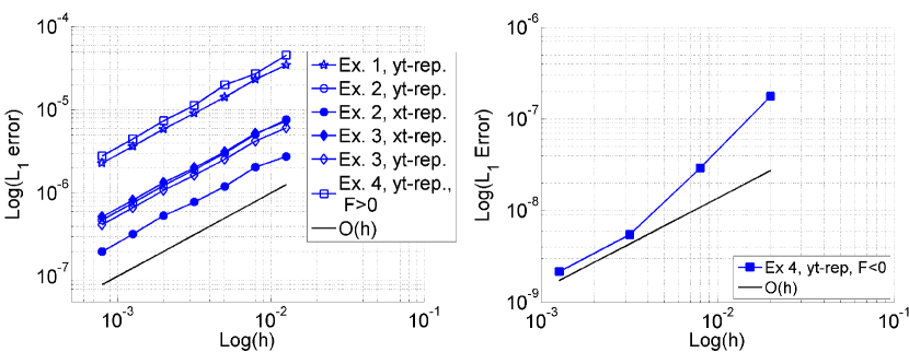
Fig. 5: Convergence results for the sideways scheme, using (left) Method 1 (right) Method 2.

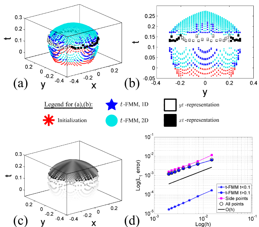
Fig. 6: Example 1: (a) - (b) Different perpectives of the set Accepted. (c) Accepted is featured. The relative error $e_{ij}$ determines the shade of each point. (d) Convergence results.

8.5 Example 2: $F=F(x)=x$

The given speed is such that the curve remains a circle whose radius grows while its center shifts to the right. Our method adequately handles this case as a single problem, although the speed changes sign across the $y$-axis. As expected, Algorithm 3 fails near the points $(0,0.25)$ and $(0,-0.25)$, as shown on Figure 7 (a). The sideways scheme was tested both in the $xt$- and the $yt$-charts, and was found to be $1^{\mathrm{st}}$ order in each case (Figure 5). The results for the full scheme show that it converges with $\mathcal{O}(h)$ accuracy everywhere (Figure 7 (b)). Let us bring up that a bi-directional FMM was proposed in [13] to solve a related problem.

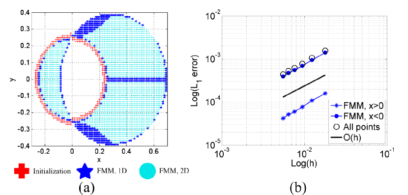
Fig. 7: Example 2: (a) The set Accepted (b) Convergence results.

8.6 Example 3: $F=F(x,y,t)$

(See Appendix C.5 for details about $F$.) This example differs significantly from the previous ones in that the set $\mathcal{F}$ no longer consists of planes. The exact solution $\mathcal{C}_{t}$ is a circle that only grows at first, and then starts moving in the positive $x$-direction. Our method is observed to perform very well on this example; We present the resulting surface and the first order convergence results on Figures 5 & 8.

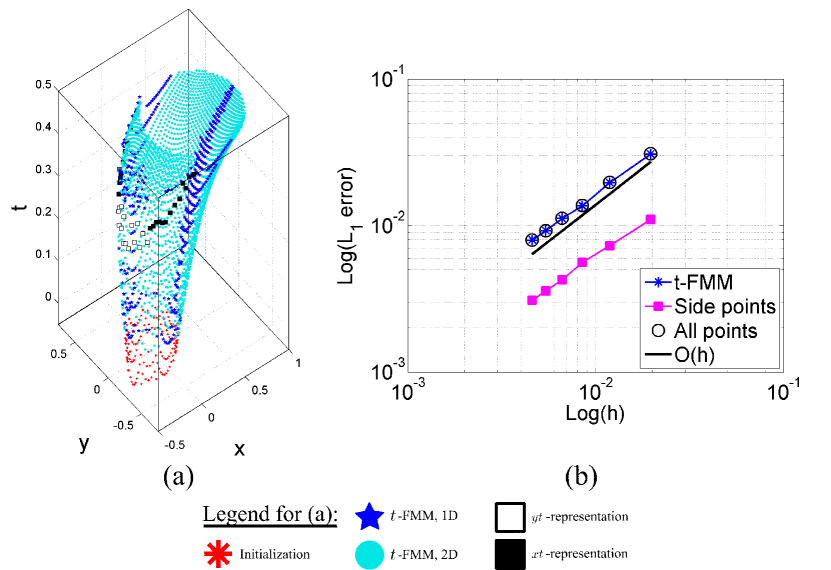
Fig. 8: Example 3: (a) The set Accepted (b) Convergence results.

8.7 Example 4: Two merging circles

This example tests the ability of the scheme to capture topological changes. The initial codimension-one manifold consists of two disjoint circles of radius $r_{0}=1/4$, with centres at $(-.3,0)$ and $(.3,0)$. The speed is such that the circles first expand, until they touch and merge. Then the speed changes sign, which makes the curve shrink until it pinches off and splits into two distinct curves. The set Accepted is presented in Figure 9 (a).The accuracy of the sideways scheme is investigated on a domain that comprises the shock when $F>0$, and the rarefaction when $F<0$. First order convergence is obtained in each case (Figure 5). The full scheme also shows $1^{\mathrm{st}}$ order convergence (Figure 9 (b)). The convergence of the sideways points and the top part is a little shy of first order, but this can be attributed to the measurement method. Those results demonstrate how robust the overall scheme is. Note that a similar example was tackled in [9], with a speed $F$ that depended linearly on time.

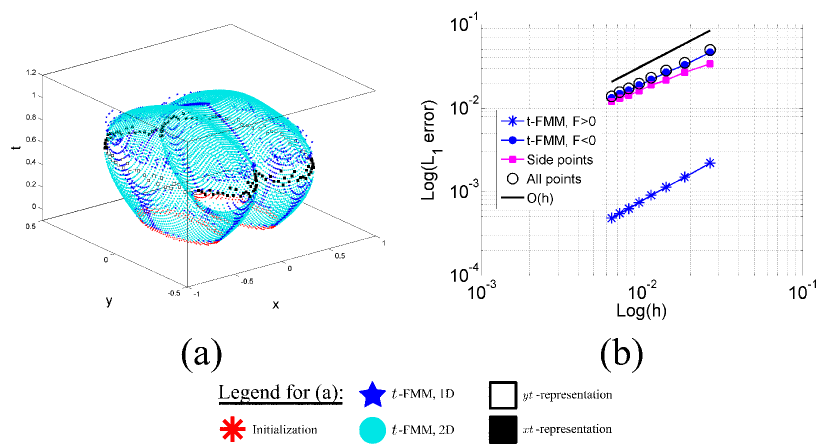
Fig. 9: Example 4: (a) The set Accepted. (b) Convergence results.

9 Discussion

In the light of the examples presented in the previous section, we address the limitations, weaknesses and advantages of the algorithm.

We illustrate one of the main limitation of the scheme with an ultimate example. The speed is chosen such that the initial circle immediately develops a kink along the $x$-axis at time $t=0$. Its subsequent shape resembles that of an almond slowly turning in the counterclockwise direction while expanding. The sign of the speed changes, forcing the curve to contract while retaining its slanted shape. See Appendix C.7 for details. The most prominent feature of this example is that, as is depicted on Figure 10, the shock is not a straight line. Remark that the speed $F$ does not satisfy the assumptions of this paper outlined in §2.2: It is only a $C^{0}$ function of $\mathbb{R}^{2}\times[0,T]$. The surface that results from running the algorithm at high resolution is shown on Figure 11. The shock is clearly visible, and has the expected figure-eight shape. Nevertheless some points ‘escape’ through the shock when the speed changes sign, and start out two new fronts that keep on expanding. The problem stems from the procedure ‘Update Pile’ in Algorithm 1. In order to decide which points go in Pile, the code distinguishes between the inside and the outside of the curve using the normal $\hat{\mathfrak{n}}$ (cf. line 12 of Algorithm 1). Consider what happens along the shock, where $\hat{\mathfrak{n}}$ has a discontinuity. So long as the expansion is outwards, this does not cause problems. But when the direction of propagation reverses, some points that should stay in Far Away are moved into Pile. A possible remedy to this issue is to approximate the normal cone along the shock. This additional information could be used as an updating criterion.

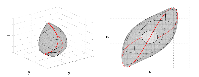
Fig. 10: $\mathcal{M}$ for the almond example. The shock appears as a red plain line.

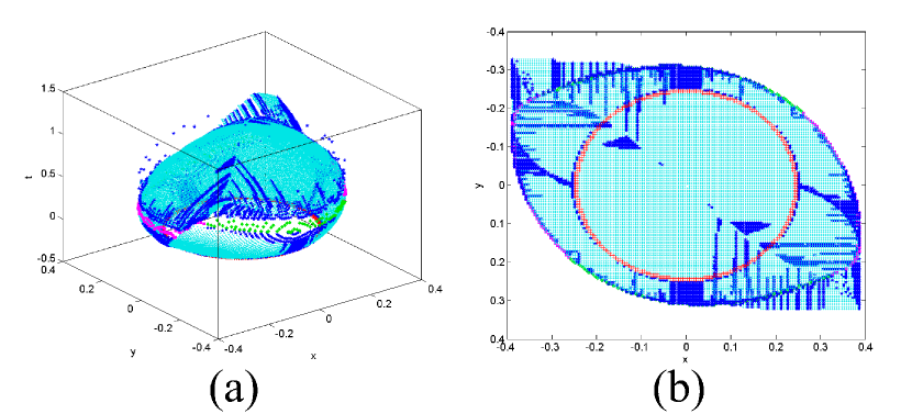
Fig. 11: The almond example: The set Accepted (a) side view, (b) viewed from above.

On a much more general note, the gluing mechanism between the two formalisms heavily relies on an accurate computation of the normal. In practice, we found that the algorithm is rather sensitive to the accuracy of this quantity. Another weakness of the method is that, as it stands, Algorithm 3 may fail when it is not supposed to. i.e., Even though $(x_{i},y_{j})$ or $(x_{\alpha},y_{\beta})$ belongs to $\mathcal{C}_{t}$ for some $t\in(0,T)$, the algorithm does not assign any value to either of those coordinates. Two situations make such a scenario possible: (1) the time steps taken are too small, or (2) too little information obtained from interpolation is available. Recall from Proposition 3 that the CFL condition prevents large $\Delta t$. Case (2) can occur if $s\in\mathbb{N}$, the number of points in the local grid in Algorithm 3 is too small. However, if $s$ is large, Algorithm 3 may not be able to carry out the step outlined in line 13. This happens if the points in NeighSide$(p_{\alpha\beta})$ sample more than one connected component of the set $\{p\in\mathcal{M}:\pi_{s}(p)\in[x_{i-s},x_{i+s}]\times[y_{j-s},y_{j+s}]\}$. See Figure 12 for an illustration. However, choosing $s$ systematically so as to prevent this situation seems difficult. Ultimately $h$ and $s$ depend on measurable quantities such as the Lipschitz constants of $F$ and its derivatives, as well as the local curvatures of $\Gamma_{t}$. Nevertheless the way those parameters are intertwined and should be chosen is a question we wish to address in future work.

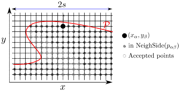
Fig. 12: Illustration of what happens if $s$ is chosen too large. Data need to be converted to the $xt$-representation, but the set NeighSide$(p_{\alpha\beta})$ of neighbours of the black point $(x_{\alpha},y_{\beta})$ consists of two connected components.

The fact that our method is a rather mild modification of the standard FMM has obvious benefits. As featured in all the examples, the sideways representations need only be used to compute a relatively small number of points sampling $\mathcal{M}$. This allows us to safely predict that the computational complexity of the algorithm is lower than that of pre-existing algorithms used to tackle this problem, such as the LSM or the GFMM. Nonetheless, it is hard at this point to make more precise complexity statements.

10 Conclusion

Our aim was to devise an algorithm with low complexity able to describe the non-linear evolution of codimension one manifolds subject to a space- & time-dependent speed function that changes sign. To this end, we illustrated how pre-existing methods can be combined to achieve this goal. The fact that we always dealt with explicit representations of the manifold implied that the dimensionality of the problem was never raised. The resulting algorithm was found to have a global truncation error of $\mathcal{O}(h)$. We tested it against a number of examples, some of which cannot be found in the current literature.

The algorithm is found to be robust and accurate in all the tests presented. Regarding the complexity of the method, a legitimate concern is to clearly quantify how the success rate of Algorithm 3 depends on the various parameters involved, as well as the speed function $F$ and the manifold $\mathcal{M}$. Once this is done, more precise statements about the runtime of the algorithm can be made and tested.

Overall, the present work thoroughly introduces a new algorithm, along with proofs of convergence and stability, as well as sturdy numerical results. We believe that the main idea on which it relies – i.e., to change representation based on the speed function $F$ – may be extended and improved in many ways that shall be explored.

Appendix A A direct method to compute $\psi_{\mathrm{II}}$ in the $t$-FMM, in 2D

We provide a direct method for solving the minimization problem appearing in Equation (35), in two dimensions. Introducing $\tau(y)=\frac{h}{|F(\vec{\mathbf{x}}_{ij},\psi(y))|}$, we first use linear interpolation to simplify the quantity we wish to minimize:

$$\psi(\tilde{\mathbf{x}})+\sqrt{\xi^{2}+(1-\xi)^{2}}~{}\frac{~{}h}{|F(\vec{\mathbf{x}}_{ij},\psi(\tilde{\mathbf{x}}))|}~{}=~{}\psi(\tilde{\mathbf{x}})+\sqrt{\xi^{2}+(1-\xi)^{2}}~{}\tau(\tilde{\mathbf{x}})$$ (76)

$$\approx \xi\psi(\vec{\mathbf{x}}_{i-1,j})+(1-\xi)\psi(\vec{\mathbf{x}}_{i,j+1})+\sqrt{\xi^{2}+(1-\xi)^{2}}~{}\left(\xi\tau(\vec{\mathbf{x}}_{i-1,j})+(1-\xi)\tau(\vec{\mathbf{x}}_{i,j+1})\right)$$

$$=: f(\xi)$$

Minimizing $f$ over $\xi\in(0,1)$ amounts to finding the roots of $0=c_{4}\lambda^{4}+c_{3}\lambda^{3}+c_{2}\lambda^{2}+c_{1}\lambda+c_{0}$ where $\lambda\in(0,1)$ is such that $f^{\prime}(\lambda)=0$. This quartic can be solved either directly with closed formulas, or with Newton’s method — we use the latter. For each root $r_{i}\in(0,1)$ the corresponding value of $\psi$ is computed as $\psi_{\mathrm{II},r_{i}}=f(r_{i})$. If $\psi_{\mathrm{II},r_{i}}<\psi(\vec{\mathbf{x}}_{i-1,j})$ or $\psi_{\mathrm{II},r_{i}}<\psi(\vec{\mathbf{x}}_{i,j+1})$, then $\psi_{\mathrm{II},r_{i}}$ is discarded. Values arising from minimization in one dimension are also computed as $\psi_{\mathrm{II},0}=\psi(\vec{\mathbf{x}}_{i,j+1})+\tau(\vec{\mathbf{x}}_{i,j+1})$ and $\psi_{\mathrm{II},1}=\psi(\vec{\mathbf{x}}_{i-1,j})+\tau(\vec{\mathbf{x}}_{i-1,j})$. The global minimum is found by comparing all those values.

Appendix B Algorithm 5, standard FMM

We revisit the standard Fast Marching Method algorithm, using some of the notation we have introduced.

Algorithm 5 Solve $|\nabla\psi(x,y)|=\frac{1}{|F(x,y)|}$

$u_{\pm}\leftarrow\pi_{t}(p_{i\pm 1j})$ if $p_{i\pm 1j}\in\mathrm{NeighEik}((x_{i},y_{j}))$, $+\infty$ otherwise.

$v_{\pm}\leftarrow\pi_{t}(p_{ij\pm 1})$ if $p_{ij\pm 1}\in\mathrm{NeighEik}((x_{i},y_{j}))$, $+\infty$ otherwise.

$u\leftarrow\min(u_{-},u_{+})$,        $v\leftarrow\min(v_{-},v_{+})$,  

if $\max(u,v)-\min(u,v)<\frac{h}{|F(x_{i},y_{j})|}$ then

     $\psi_{ij}=\frac{1}{2}\left((u+v)+\sqrt{2\left(\frac{h}{F(x_{i},y_{j})}\right)^{2}-(u-v)^{2}}\right)$

else

     $\psi_{ij}=\min(u,v)+\frac{h}{|F(x_{i},y_{j})|}$

Appendix C Implementation details for the examples

C.1 Solvers used

We give some details about the examples presented in §8. All tests were performed using Matlab^® [1]. In particular, finding the minimum value in the Narrow Band is done using the command

in ~.
%\paragraph{Initialization} All data are initialized with exact values.
%\paragraph{Interpolation} The interpolation sche

e that converts data from one representation to another is one-dimensional linear interpolation, as illustrated on Figure 4. This procedure is $\mathcal{O}(h)$.

Whenever a value $\psi_{ij}$ is computed by the $(t)$-FMM, the normal $\hat{n}_{ij}$ is approximated using the one-sided derivatives involving the points used in the computation of $\psi_{ij}$. For example: if two-dimensional optimization was used in Quadrant III to obtain $\psi_{ij}$, then

$$\vec{v}=\left(\frac{\psi_{ij}-\psi_{i-1,j}}{h},\frac{\psi_{ij}-\psi_{i,j-1}}{h},-\mathrm{\textsl{Orient}3~{}}(p_{ij})\right)\quad\mathrm{and}\quad\hat{n}(p_{ij})=\frac{\vec{v}}{|\vec{v}|}$$ (77)

Within Algorithm 3, we approximate the normal as follows. For clarity, say the points $p^{k}_{j}=(\psi^{k}_{j},y_{j},t^{k})$ and $p^{k-1}_{j}=(\psi^{k-1}_{j},y_{j},t^{k-1})$ computed in the $yt$-representation with $x$-orientation $a$ were used to obtain $p_{ij}=(x_{i},y_{j},\psi_{ij})$. Then

$$\vec{v}=\left(-a,a~{}\frac{\psi^{k-1}_{j+1}-\psi^{k-1}_{j-1}}{2h},a~{}\frac{\psi^{k}_{j}-\psi^{k-1}_{j}}{dt}\right)\quad\mathrm{and}\quad\hat{n}(p_{ij})=\frac{\vec{v}}{|\vec{v}|}$$ (78)

Note that this is not an approximation of the true normal at $p_{ij}$, which is $(-a,-\phi_{x}\psi_{y},$ $-\phi_{x}\psi_{t})$. However, the only two salient information we need from $\hat{n}$ are: the sign of $\hat{n}_{3}$ and the direction of $\hat{\mathfrak{n}}$. The two-dimensional normal is simply obtained from $\hat{n}$ as $\hat{\mathfrak{n}}=\frac{(\hat{n}_{1},\hat{n}_{2})}{|(\hat{n}_{1},\hat{n}_{2})|}$.

C.2 Choice of parameters

In all examples, the number of points in each dimension is $N+1$, and the spatial grid spacings are even: $h=dx=dy$. The size of the local grid in Algorithm 3 was set to be $s=\lfloor\frac{N}{3}\rfloor$. As discussed in §6.2.3, we use adaptive time-stepping, in those examples where $F$ depends on time. In the fine part, before the time where $F=0$, we set $\Delta t=r_{1}h$. Passed that time, we let $\Delta t=r_{2}h$. To assess the convergence of the sideways methods, a $yt$-grid with spacings $h$ and $\Delta t=h/2$ was built.Remark that the exact normal $\hat{n}$ was assigned to the points as they were accepted in all the examples, except Example 1 where it was computed as explained in §C.1.

C.3 Example 1

The exact solution to the Level-Set Equation is $\phi(x,y,t)=\sqrt{x^{2}+y^{2}}-R(t)$ where $R(t)=\left(r_{0}-\frac{e^{10t}-1}{10e}+t\right)$. Domain: $[-.321,.319]^{2}$. $T_{F}=0.3$. $xt$- and $yt$-rep.: $r_{1}=1/3$, $r_{2}=2$. Skewed rep.: $r_{1}=r_{2}=1$. Domain for convergence of Algo. 4: $(y,t)\in[-0.25,0.25]\times[0,0.3]$.

C.4 Example 2

The signed distance function to the curve $\mathcal{C}_{t}$ is given as $\phi(x,y,t)=\sqrt{(x-x_{c}(t))^{2}+y^{2}}-r(t)$ where $x_{c}(t)=r_{0}\sinh t$ and $r(t)=r_{0}\cosh t$. Note that $\phi$ does not solve the Level-Set Equation. Domain: $[-1.01,0.99]^{2}$. $T_{F}=1$. $xt$- and $yt$-rep.: $r_{1}=1/3$, $r_{2}=2$. Skewed rep.: $r_{1}=1/3$, $r_{2}=5$. Domain for convergence of Algo. 4: $(y,t)\in[-0.25,0.25]\times[0,1]$ and $(x,t)\in[-0.25,0.25]\times[0,1]$.

C.5 Example 3

The exact solution to the Level-Set Equation is $\phi(x,y,t)=\sqrt{(x-gt)^{2}+y^{2}}-\left(r_{0}+ct\right)$ where $b=10$, $c=1/2$ and $g(t)=\arctan\left(b(t-0.5)\right)+\frac{\pi}{2}$. The speed is

$$F=\frac{(x-gt)(g^{\prime}t+g)}{\sqrt{(x-gt)^{2}+y^{2}}}+c~{}\Longrightarrow~{}F\approx\left\{\begin{array}[]{ll}c&\mathrm{for~{}}t\mathrm{~{}small}\\ \frac{(x-\pi t)\pi}{\sqrt{(x-\pi t)^{2}+y^{2}}}+c&\mathrm{for~{}}t\mathrm{~{}large}\\ \end{array}\right.$$ (81)

We expect the circle to first expand (when $t$ is small), and then expand while moving to the right with speed $\pi$ (when $t$ is large). Domain: $[-1.51,+1.49]^{2}$. $T_{F}=0.5$. $xt$- and $yt$-rep.: $r_{1}=1/3$, $r_{2}=2$. Skewed rep.: $r_{1}=1/3$, $r_{2}=5$. Domain for convergence of Algo. 4: $(y,t)\in[-0.25,0.25]\times[0,0.5]$.

C.6 Example 4

The set $\mathcal{C}_{0}$ consists of two disjoint circles of radius $r_{0}=0.25$, with centres at $(-0.3,0)$ and $(0.3,0)$. The speed is $F=1-e^{2t-1}$. The circles touch along the $y$-axis when $t\approx 0.08$. When $t<0.5$ the exact solution to the Level-Set Equation is $\phi(x,y,t)=\min\left\{\sqrt{(x+0.3)^{2}+y^{2}}-R(t),\sqrt{(x-0.3)^{2}+y^{2}}-R(t)\right\}$ where $R(t)=r_{0}-\frac{e^{2t}-1}{2e}+t$. Domain: $[-1.5+0.01e,+1.5+0.01e]^{2}$. $T_{F}=1.2$. $xt$- and $yt$-rep.: $r_{1}=1/3$, $r_{2}=2$. Skewed rep.: $r_{1}=1/3$, $r_{2}=5$. Domain for convergence of Algo. 4: $(y,t)\in[-0.5,0.5]\times[0.2,0.5]$ and $(y,t)\in[-0.5,0.5]\times[0.5,.52]$.

C.7 The Almond example

The exact solution to the Level-Set Equation is

$$\phi(x,y,t) = \left(\sqrt{x^{2}+y^{2}}-r_{0}+\frac{e^{ct}-1}{ce}-t(1+C)\right)+\frac{t|xt-y|}{\sqrt{1+t^{2}}}$$ (82)

$$=: \tilde{\phi}(x,y,t)+g(x,y,t)$$ (83)

The constants are set to be: $r_{0}=1/4$, $c=1$, and $C=.65$. The function $\phi$ is made up of two parts: $\tilde{\phi}$ is qualitatively the same as in Example 1. Domain: $[-0.5,0.5]^{2}$. $T_{F}=1.9$. $xt$- and $yt$-rep.: $r_{1}=1/3$, $r_{2}=2$. Skewed rep.: $r_{1}=1/2$, $r_{2}=6$.

Acknowledgements The authors wish to thank Prof. A.Oberman for helpful discussions. The second author would like to thank the organizers of the 2011 BIRS workshop “Advancing numerical methods for viscosity solutions and applications”, Profs. Falcone, Ferretti, Mitchell, & Zhao for stimulating discussions which eventually lead to the present work.

References

- [1] MatLab and Statistics Toolbox Release 2010b, Version 7.11.0.584. The Mathworks, Inc., Natick, Massachusetts, United States.
- [2] D. Adalsteinsson and J. A. Sethian. A level set approach to a unified model for etching, deposition, and lithography. I. Algorithms and two-dimensional simulations. J. Comput. Phys., 120(1):128–144, 1995.
- [3] D Adalsteinsson and JA Sethian. A level set approach to a unified model for etching, deposition, and lithography II: Three-dimensional simulations. Journal of computational physics, 122(2):348–366, 1995.
- [4] D Adalsteinsson and JA Sethian. A level set approach to a unified model for etching, deposition, and lithography III: Redeposition, reemission, surface diffusion, and complex simulations. Journal of computational physics, 138(1):193–223, 1997.
- [5] David Adalsteinsson and James A. Sethian. A fast level set method for propagating interfaces. J. Comput. Phys., 118(2):269–277, 1995.
- [6] Nina Amenta, Marshall Bern, and Manolis Kamvysselis. A new Voronoi-based surface reconstruction algorithm. In Proceedings of the 25th Annual Conference on Computer Graphics and Interactive Techniques, SIGGRAPH ’98, pages 415–421, New York, NY, USA, 1998. ACM.
- [7] M. Bardi and I. Capuzzo-Dolcetta. Optimal Control and Viscosity Solutions of Hamilton-Jacobi-Bellman Equations. Modern Birkhäuser Classics. Birkhäuser Boston, 2008.
- [8] G. Barles. Existence results for first order Hamilton Jacobi equations. Ann. Inst. H. Poincaré Anal. Non Linéaire, 1(5):325–340, 1984.
- [9] E. Carlini, M. Falcone, N. Forcadel, and R. Monneau. Convergence of a generalized fast-marching method for an eikonal equation with a velocity-changing sign. SIAM J. Numer. Anal., 46(6):2920–2952, 2008.
- [10] Frédéric Chazal, David Cohen-Steiner, and Quentin Mérigot. Geometric inference for probability measures. Found. Comput. Math., 11(6):733–751, 2011.
- [11] Li-Tien Cheng and Yen-Hsi Tsai. Redistancing by flow of time dependent eikonal equation. J. Comput. Phys., 227(8):4002–4017, 2008.
- [12] David L Chopp. Some improvements of the fast marching method. SIAM Journal on Scientific Computing, 23(1):230–244, 2001.
- [13] David L Chopp. Another look at velocity extensions in the level set method. SIAM Journal on Scientific Computing, 31(5):3255–3273, 2009.
- [14] M. G. Crandall, L. C. Evans, and P.-L. Lions. Some properties of viscosity solutions of Hamilton-Jacobi equations. Trans. Amer. Math. Soc., 282(2):487–502, 1984.
- [15] Michael G. Crandall, Hitoshi Ishii, and Pierre-Louis Lions. User’s guide to viscosity solutions of second order partial differential equations. Bull. Amer. Math. Soc. (N.S.), 27(1):1–67, 1992.
- [16] Michael G Crandall and P-L Lions. Two approximations of solutions of Hamilton-Jacobi equations. Mathematics of Computation, 43(167):1–19, 1984.
- [17] Michael G Crandall and Pierre-Louis Lions. Viscosity solutions of Hamilton-Jacobi equations. Transactions of the American Mathematical Society, 277(1):1–42, 1983.
- [18] Michael G. Crandall and Luc Tartar. Some relations between nonexpansive and order preserving mappings. Proc. Amer. Math. Soc., 78(3):385–390, 1980.
- [19] E.W. Dijkstra. A note on two problems in connexion with graphs. Numerische Mathematik, 1(1):269–271, 1959.
- [20] L. C. Evans and J. Spruck. Motion of level sets by mean curvature. I. J. Differential Geom., 33(3):635–681, 1991.
- [21] L. C. Evans and J. Spruck. Motion of level sets by mean curvature. II. Trans. Amer. Math. Soc., 330(1):321–332, 1992.
- [22] L. C. Evans and J. Spruck. Motion of level sets by mean curvature. III. J. Geom. Anal., 2(2):121–150, 1992.
- [23] Lawrence C. Evans and Joel Spruck. Motion of level sets by mean curvature. IV. J. Geom. Anal., 5(1):77–114, 1995.
- [24] L.C. Evans. Partial Differential Equations. Graduate studies in mathematics. American Mathematical Society, 2010.
- [25] M Falcone. The minimum time problem and its applications to front propagation. Motion by Mean Curvature and Related Topics, pages 70–88, 1994.
- [26] Frédéric Gibou, Ronald Fedkiw, Russel Caflisch, and Stanley Osher. A level set approach for the numerical simulation of dendritic growth. J. Sci. Comput., 19(1-3):183–199, 2003. Special issue in honor of the sixtieth birthday of Stanley Osher.
- [27] Hugues Hoppe, Tony DeRose, Tom Duchamp, John McDonald, and Werner Stuetzle. Surface reconstruction from unorganized points. SIGGRAPH Comput. Graph., 26(2):71–78, July 1992.
- [28] S. Koike. A Beginner’s Guide to the Theory of Viscosity Solutions. MSJ Memoirs. Mathematical Society of Japan, 2004.
- [29] Pierre-Louis Lions, Elisabeth Rouy, and A Tourin. Shape-from-shading, viscosity solutions and edges. Numerische Mathematik, 64(1):323–353, 1993.
- [30] William E. Lorensen and Harvey E. Cline. Marching cubes: A high resolution 3D surface construction algorithm. SIGGRAPH Comput. Graph., 21(4):163–169, August 1987.
- [31] Ravikanth Malladi, James A. Sethian, and Baba C. Vemuri. A fast level set based algorithm for topology-independent shape modeling. J. Math. Imaging Vision, 6(2-3):269–289, 1996.
- [32] Barry Merriman, James K. Bence, and Stanley J. Osher. Motion of multiple functions: a level set approach. J. Comput. Phys., 112(2):334–363, 1994.
- [33] W. Mulder, S. Osher, and James A. Sethian. Computing interface motion in compressible gas dynamics. J. Comput. Phys., 100(2):209–228, 1992.
- [34] Adam M. Oberman. Convergent difference schemes for degenerate elliptic and parabolic equations: Hamilton-Jacobi equations and free boundary problems. SIAM J. Numer. Anal., 44(2):879–895 (electronic), 2006.
- [35] S. Osher and J. Sethian. Fronts propagating with curvature dependent speed: algorithms based on Hamilton-Jacobi formulations. J. Comp. Phys., 79:12–49, 1988).
- [36] Stanley Osher, Li-Tien Cheng, Myungjoo Kang, Hyeseon Shim, and Yen-Hsi Tsai. Geometric optics in a phase-space-based level set and eulerian framework. Journal of Computational Physics, 179(2):622 – 648, 2002.
- [37] Stanley Osher and Ronald Fedkiw. Level set methods and dynamic implicit surfaces, volume 153 of Applied Mathematical Sciences. Springer-Verlag, New York, 2003.
- [38] Mark Pauly, Markus Gross, and Leif P. Kobbelt. Efficient simplification of point-sampled surfaces. In Proceedings of the Conference on Visualization ’02, VIS ’02, pages 163–170, Washington, DC, USA, 2002. IEEE Computer Society.
- [39] Danping Peng, Barry Merriman, Stanley Osher, Hongkai Zhao, and Myungjoo Kang. A PDE-based fast local level set method. J. Comput. Phys., 155(2):410–438, 1999.
- [40] Giovanni Russo and Peter Smereka. A remark on computing distance functions. J. Comput. Phys., 163(1):51–67, 2000.
- [41] J. Sethian. A fast marching level set method for monotonically advancing fronts. Proc. Natl. Acad. Sci., 93:1591–1595, 1996.
- [42] J. Sethian. Fast marching methods. SIAM Review, 41(2):199–235, 1999.
- [43] J. A. Sethian and A. Vladimirsky. Ordered upwind methods for static Hamilton-Jacobi equations. Proc. Natl. Acad. Sci. USA, 98(20):11069–11074, 2001.
- [44] J.A. Sethian. Level Set Methods and Fast Marching Methods: Evolving Interfaces in Computational Geometry, Fluid Mechanics, Computer Vision, and Materials Science. Cambridge Monographs on Applied and Computational Mathematics. Cambridge University Press, 1999.
- [45] James A. Sethian and John Strain. Crystal growth and dendritic solidification. J. Comput. Phys., 98(2):231–253, 1992.
- [46] James A. Sethian and Alexander Vladimirsky. Ordered upwind methods for static Hamilton-Jacobi equations: theory and algorithms. SIAM J. Numer. Anal., 41(1):325–363, 2003.
- [47] JamesA. Sethian. Numerical methods for propagating fronts. In Paul Concus and Robert Finn, editors, Variational Methods for Free Surface Interfaces, pages 155–164. Springer New York, 1987.
- [48] Panagiotis E Souganidis. Approximation schemes for viscosity solutions of Hamilton-Jacobi equations. Journal of differential equations, 59(1):1–43, 1985.
- [49] Panagiotis E. Souganidis. Existence of viscosity solutions of Hamilton-Jacobi equations. J. Differential Equations, 56(3):345–390, 1985.
- [50] A.I. Subbotin. Generalized Solutions of First Order PDEs: The Dynamical Optimization Perspective. Systems & Control. Birkhäuser Boston, 1994.
- [51] Mark Sussman and Emad Fatemi. An efficient, interface-preserving level set redistancing algorithm and its application to interfacial incompressible fluid flow. SIAM J. Sci. Comput., 20(4):1165–1191 (electronic), 1999.
- [52] Mark Sussman, Peter Smereka, and Stanley Osher. A level set approach for computing solutions to incompressible two-phase flow. Journal of Computational physics, 114(1):146–159, 1994.
- [53] R. Takei and R. Tsai, Y.-H. Optimal trajectories of curvature constrained motion in hamilton-jacobi formulation (to appear). J. Sci. Comput., 2013.
- [54] John N. Tsitsiklis. Efficient algorithms for globally optimal trajectories. IEEE Trans. Automat. Control, 40(9):1528–1538, 1995.
- [55] A. Vladimirsky. Static PDEs for time-dependent control problems. Interfaces Free Bound., 8(3):281–300, 2006.
- [56] Hong-Kai Zhao, S. Osher, and R. Fedkiw. Fast surface reconstruction using the level set method. In Variational and Level Set Methods in Computer Vision, 2001. Proceedings. IEEE Workshop on, pages 194 –201, 2001.
- [57] Hongkai Zhao. A fast sweeping method for Eikonal equations. Mathematics of computation, 74(250):603–627, 2005.
- [58] J Zhu and PD Ronney. Simulation of front propagation at large non-dimensional flow disturbance intensities. Combustion science and technology, 100(1-6):183–201, 1994.