Redshift-Space Clustering of SDSS Galaxies — Luminosity Dependence, Halo Occupation Distribution, and Velocity Bias

Abstract

We present the measurements and modelling of the small-to-intermediate scale ($\sim 0.1$–$25\,h^{-1}{\rm{Mpc}}$) projected and three-dimensional (3D) redshift-space two-point correlation functions (2PCFs) of local galaxies in the Sloan Digital Sky Survey (SDSS) Data Release 7. We find a clear dependence of galaxy clustering on luminosity in both projected and redshift spaces, generally being stronger for more luminous samples. The measurements are successfully interpreted within the halo occupation distribution (HOD) framework with central and satellite velocity bias parameters to describe galaxy kinematics inside haloes and to model redshift-space distortion (RSD) effects. In agreement with previous studies, we find that more luminous galaxies reside in more massive haloes. Including the redshift-space 2PCFs helps tighten the HOD constraints. Moreover, we find that luminous central galaxies are not at rest at the halo centres, with the velocity dispersion about 30% that of the dark matter. Such a relative motion may reflect the consequence of galaxy and halo mergers, and we find that central galaxies in lower mass haloes tend to be more relaxed with respect to their host haloes. The motion of satellite galaxies in luminous samples is consistent with their following that of the dark matter. For faint samples, satellites tends to have slower motion, with velocity dispersion inside haloes about 85% that of the dark matter. We discuss possible applications of the velocity bias constraints on studying galaxy evolution and cosmology. In the appendix, we characterize the distribution of galaxy redshift measurement errors, which is well described by a Gaussian-convolved double exponential distribution.

1 Introduction

The three-dimensional galaxy distribution in our Universe can be probed through the large-scale galaxy redshift surveys, such as the Sloan Digital Sky Survey (SDSS; York et al., 2000). The angular positions of the galaxies can be accurately measured in photometric observations, while the radial positions are usually obtained from the observed galaxy redshifts. However, the radial distances derived from the redshifts differ from the real positions of galaxies due to the existence of the galaxy peculiar velocities, which is usually referred to as the redshift-space distortion (RSD) effect. Although the RSD prevents us from measuring the true galaxy distribution, it also provides valuable information about the galaxy kinematics in dark matter haloes.

A commonly used statistic for analysing the galaxy distribution is the three-dimensional (3D) two-point correlation function (2PCF), $\xi(r_{p},r_{\rm\pi})$, where $r_{p}$ and $r_{\rm\pi}$ are the transverse and line-of-sight (LOS) separations of galaxy pairs, respectively (see e.g. Zehavi et al., 2005, 2011; Li et al., 2006; Guo et al., 2013). To minimise the effect of RSD, the traditional way of probing the real-space galaxy distribution is through the projected 2PCF, $w_{p}(r_{p})$, by integrating $\xi(r_{p},r_{\rm\pi})$ along the LOS direction. Since $w_{p}(r_{p})$ is insensitive to the galaxy peculiar velocities, it only probes the galaxy spatial distribution. To fully understand the galaxy phase-space distribution, we need to model the redshift-space clustering of galaxies.

In contemporary galaxy formation and evolution models, galaxies form and evolve in dark matter haloes. The galaxy distribution in the universe can then be studied with the halo model, through the distribution of galaxies within the haloes and the halo distributions in the large-scale structure of the universe (see e.g. Cooray & Sheth, 2002, and references therein). Since the distribution of dark matter haloes is well understood using analytic models and numerical $N$-body simulations (e.g., Mo et al., 1996; Springel, 2005; Klypin et al., 2014), the key component of the models is the connection between galaxies and dark matter haloes, such as the framework of halo occupation distribution (HOD) or the closely related conditional luminosity function (e.g. Jing et al., 1998; Peacock & Smith, 2000; Seljak, 2000; Scoccimarro et al., 2001; Berlind & Weinberg, 2002; Yang et al., 2003; Zheng et al., 2005; Guo et al., 2014; Skibba et al., 2015). The HOD describes the probability distribution $P(N|M)$ of having $N$ galaxies of a given type in a dark matter halo of virial mass $M$. The probability distribution $P(N|M)$, together with the spatial and velocity distributions of galaxies inside haloes, is crucial to interpret and understand the real- and redshift-space clustering of galaxies. The observationally inferred HOD can help us test and constrain galaxy formation models.

A large fraction of the information contents on the HOD (like the occupation function and galaxy kinematics and spatial distribution inside haloes) are contained in the small-scale clustering of galaxies. However, both measuring and modelling the galaxy distribution are nontrivial in the small-scale nonlinear regime. On the observational side, in fibre-fed spectrograph surveys as in the SDSS, the hardware limit that two fibres on the same plate cannot be placed closer than an angular separation of $55^{\prime\prime}$ (Blanton et al., 2003a) significantly hinders the number of close galaxy pairs on small scales. Fortunately, this fibre collision effect can be accurately corrected using the method of Guo, Zehavi & Zheng (2012), by taking advantage of the recovered redshifts of collided galaxies in the plate-overlap regions. On the theory side, modelling the galaxy distributions on small scales is also difficult, especially in redshift space due to the lack of understanding of the galaxy phase-space distribution. This problem can be alleviated with the help of high-resolution $N$-body dark matter simulations.

Recently, Guo et al. (2015) (hereafter G15) measured and modelled the luminous red galaxy (LRG) distribution in the SDSS-III Baryon Oscillation Spectroscopic Survey (BOSS; Eisenstein et al., 2011; Dawson et al., 2013) at redshift $z{\sim}0.5$, and found that central galaxies are not at rest at the halo centres and the satellite galaxies move more slowly than the dark matter. The difference in galaxy and matter velocity distributions is dubbed as velocity bias. In this paper, we follow the method of G15 and infer the phase-space distribution of galaxies in the local universe through modelling the redshift-space galaxy 2PCFs. We improve the model of G15 and also incorporate a more accurate redshift error model shown in Appendix A. In Section 2, we describe the data, the galaxy samples, and the redshift-space 2PCF measurements. We introduce our modelling method in Section 3. The constraints on the occupation function and galaxy phase-space distribution are presented in Section 4. Finally, we summarize our results in Section 5.

Throughout the paper, for the measurements we assume a spatially flat $\Lambda$ cold dark matter ($\Lambda$CDM) cosmology, with $\Omega_{m}=0.307$ and $h=0.678$, which is adopted in the MultiDark simulation (and model) we use, and consistent with the constraints from Planck (Planck Collaboration et al., 2014).

2 Data and Measurements

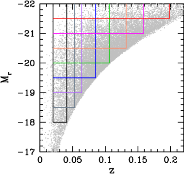
Figure 1: Construction of volume-limited galaxy samples with different luminosity thresholds. The dots show the distribution of SDSS galaxies as a function of redshift $z$ and $r$-band absolute magnitude $M_{r}$. The different colour lines delineate the selection cuts for different luminosity-threshold samples defined in Table 1.

For the purpose of studying the galaxy distribution in the local universe, we use the galaxy sample of the New York University Value-Added Galaxy Catalog (NYU-VAGC; Blanton et al., 2005), which is constructed from the SDSS Data Release 7 Main galaxy sample (Abazajian et al., 2009). The sample covers an effective area of about $7300\deg^{2}$, with galaxies selected using an $r$-band Petrosian magnitude limit of $r<17.77$. The magnitudes in the catalog are $K$–corrected and passively evolving to the median redshift of $z=0.1$ (Blanton et al., 2003b). To properly measure and model the galaxy clustering and its dependence on galaxy luminosity, we construct volume-limited samples with different luminosity thresholds. We impose a minimum redshift of $z=0.02$. The selection cuts for the different samples are shown in Fig. 1. Table 1 provides the corresponding sample information, including the average number density and the volume of each sample. Overall, the samples are similar to those constructed in Zehavi et al. (2011).

We measure the 3D redshift-space 2PCFs $\xi(r_{p},r_{\rm\pi})$ of the SDSS DR7 Main galaxy sample through the Landy–Szalay estimator (Landy & Szalay, 1993). The 2PCF, $\xi(r_{p},r_{\rm\pi})$, can be further integrated along the LOS to reduce the effect of RSD. The resulting projected 2PCF $w_{p}(r_{p})$ (Davis & Peebles, 1983) is defined as

$$w_{p}(r_{p})=2\int_{0}^{\infty}\xi(r_{p},r_{\rm\pi})dr_{\rm\pi}.$$ (1)

In both the measurements and the model, we integrate $\xi(r_{p},r_{\pi})$ to $r_{\pi,{\rm max}}=40\,h^{-1}{\rm{Mpc}}$ to obtain $w_{p}$. We adopt logarithmic $r_{p}$ bins centred at $0.13$ to $20.48\,h^{-1}{\rm{Mpc}}$ with $\Delta\log r_{p}=0.2$, and linear $r_{\rm\pi}$ bins from 0 to 40$\,h^{-1}{\rm{Mpc}}$ with $\Delta r_{\rm\pi}=2\,h^{-1}{\rm{Mpc}}$. Denoting the relative redshift-space position of a pair of galaxies as $\mn@boldsymbol{s}$, we also measure the redshift-space 2PCF in bins of $s$ and $\mu$, with $s=\sqrt{r_{p}^{2}+r_{\rm\pi}^{2}}$ being the redshift-space separation of galaxy pairs and $\mu$ being the cosine of the angle between $\mn@boldsymbol{s}$ and the LOS. The redshift-space 2PCF $\xi(s,\mu)$ can be expanded into multipoles (Hamilton, 1992),

$$\xi(s,\mu)=\sum_{l}\xi_{l}(s)P_{l}(\mu),$$ (2)

where $P_{l}$ is the $l$-th order Legendre polynomial. The multipole moments $\xi_{l}$ are usually used to characterize the redshift-space clustering (G15). We focus on the measurements of the monopole ($\xi_{0}$), quadrupole ($\xi_{2}$), and hexadecapole ($\xi_{4}$). For $s$, we adopt the same logarithmic bins as $r_{p}$, while for $\mu$ we use linear bins from -1 to 1 with $\Delta\mu=0.05$.

In linear theory, the three multipole moments we adopt are the only non-zero terms. While at any scales odd terms are zero by the symmetry of $\xi(s,\mu)$, at the translinear or nonlinear scales explored in this paper, higher-order even terms do exist. However, the information content in the higher-order terms is minimal compared to the three main terms ($\xi_{0}$, $\xi_{2}$, and $\xi_{4}$), as they are highly correlated with these lower-order terms. For example, Hikage (2014) explored the constraints on the HOD by including multipoles of different orders, and found that including the tetra-hexadecapole ($l=6$) in addition to multipoles with $l=$0, 2, and 4 leads to virtually no improvement in the constraints (see their Table 1 and Fig. 3). We therefore limit our study to only $\xi_{0}$, $\xi_{2}$, and $\xi_{4}$, in addition to $w_{p}$.

Table 1: Samples of different luminosity thresholds

$M_{r}^{\rm max}$	$z_{\rm max}$	$N$	$n_{g}$	$V$
$-18.0$	0.041	35649	$31.42\pm 4.03$	$1.19$
$-18.5$	0.053	57786	$22.25\pm 2.70$	$2.72$
$-19.0$	0.064	72484	$15.66\pm 2.06$	$4.87$
$-19.5$	0.085	125664	$11.64\pm 1.27$	$11.44$
$-20.0$	0.106	131623	$6.37\pm 0.75$	$22.00$
$-20.5$	0.132	122115	$3.13\pm 0.30$	$41.82$
$-21.0$	0.159	76802	$1.16\pm 0.12$	$71.74$
$-21.5$	0.198	35207	$0.29\pm 0.03$	$134.65$

The absolute magnitude is computed by assuming $h=1$. The minimum redshift of all the luminosity threshold samples is $z_{\rm min}=0.02$. The total number of galaxies $N$ in each sample is also displayed. The mean number density $n_{g}$ is in units of $10^{-3}h^{3}{\rm{Mpc}}^{-3}$. The volume $V$ of each sample is in units of $10^{6}h^{-3}{\rm{Mpc}}^{3}$.

We apply the method developed in Guo, Zehavi & Zheng (2012) to correct the fibre-collision effect, enabling accurate measurements of the small-scale 2PCFs. For each sample, the covariance matrix of the measurements is estimated from 400 jackknife samples (Zehavi et al., 2011; Guo et al., 2015).

We show in Fig. 2 the measured 2PCFs for the different luminosity threshold samples. It is clear from the projected 2PCF $w_{p}(r_{p})$ and the redshift-space monopole $\xi_{0}(s)$ that more luminous galaxies have stronger clustering amplitudes than their fainter counterparts, consistent with the results of Zehavi et al. (2011). The measurements of the quadrupole $\xi_{2}(s)$ and hexadecapole $\xi_{4}(s)$ are noisier, but the overall dependence on luminosity is clear. For example, more luminous galaxies show a more positive quadrupole and hexadecapole on small scales, indicating stronger Fingers-of-God (FOG) effects. We jointly model all the 2PCF measurements in the following sections.

3 Simulation and Model

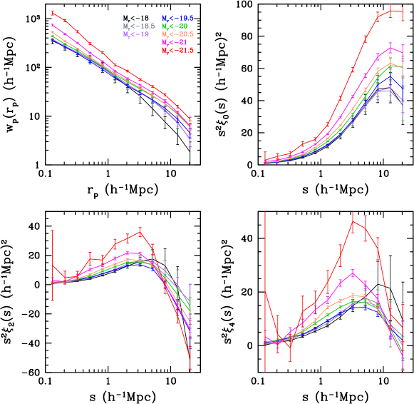
Figure 2: Measured projected 2PCF $w_{p}(r_{p})$ (top left), redshift-space monopole $\xi_{0}(s)$ (top right), quadrupole $\xi_{2}(s)$ (bottom left), and hexadecapole $\xi_{4}(s)$ (bottom right) for SDSS galaxies. The different colour lines show the measurements for different luminosity threshold samples. The errors are estimated from 400 jackknife samples.

To accurately model the galaxy clustering under the HOD framework, we follow the simulation-based model method developed in Zheng & Guo (2015), which is used in G15 to model redshift-space clustering of BOSS galaxies. It tabulates properties of haloes in an $N$-body simulation (e.g., halo mass functions, halo profiles, halo clustering) necessary for computing galaxy 2PCFs. Given a set of HOD parameters, the model can then accurately predict the galaxy 2PCFs. It is equivalent to assigning galaxies to haloes in the simulation with the given set of HOD parameters and measuring the 2PCFs from the resultant mock catalog. When populating haloes with galaxies, the redshift-space distortion is applied in a galaxy-by-galaxy manner by using the velocity information of galaxies and haloes. Our modelling method does the same thing by using the galaxy velocity distribution inside haloes and the redshift-space clustering of haloes (see Zheng & Guo 2015 for details). Our simulation-based modelling method works more efficiently than directly populating the simulation with galaxies, since it enables ‘populating galaxies’ and ‘measuring the 2PCF in the mock’ to be performed analytically. The model is accurate since it automatically takes into account the effects of halo exclusion, nonlinear growth, and scale-dependent halo bias by using the halo catalogues in high-resolution simulations. In particular, it is well suited to model the redshift-space galaxy clustering on small and intermediate scales, for which an accurate analytic model is difficult to develop (e.g. Tinker, 2007; Reid & White, 2011; Wang et al., 2014a; White et al., 2015).

The model we use in this paper is based on the MultiDark simulation of Planck cosmology (MDPL; Klypin et al. 2014), which is carried out with L-GADGET-2 code (Springel, 2005). The cosmological parameters ($\Omega_{m}=0.307$, $\Omega_{b}=0.048$, $h=0.678$, $n_{s}=0.96$, and $\sigma_{8}=0.823$) used in MDPL are consistent with the recent results from Planck (Planck Collaboration et al., 2014). The simulation has 3840³ dark matter particles in a box of 1 $h^{-1}$ Gpc (comoving) on a side, so the mass resolution is $1.51\times 10^{9}\,h^{-1}{\rm M_{\sun}}$, which is about 6 times higher than the previous MultiDark run simulation (MDR1; Prada et al. 2012). The force resolution, i.e. the gravitational softening length, is only $5h^{-1}$ kpc (physical) at low redshifts, which enables us to accurately model the clustering signals on very small scales. We use the simulation output at $z=0$ to model all the luminosity threshold galaxy samples in the NYU-VAGC. In principle, when modelling the measurements, it is better to choose the simulation output to match the mean redshift for each individual sample. This is certainly limited by the available simulation outputs. On the other hand, given the small redshift range of the SDSS Main galaxies, the effect of using one output (as we do) is small. We have tested applying the $z=0.1$ simulation output for modelling the data, and the inferred HOD parameters are consistent with those from the default model built on the $z=0$ output.

Dark matter haloes are identified using the Rockstar phase-space halo finder (Behroozi et al., 2013), which is efficient and accurate in finding the bound spherical structures from the density peaks in the phase space (Onions et al., 2012; Knebe et al., 2013). Halo mass is defined from the given spherical overdensities of a virial structure (Bryan & Norman, 1998). Note that we do not remove the unbound particles in the haloes, because the satellite galaxies in the haloes can also be unbound. The halo positions, velocities and velocity dispersions are calculated from all the particles in the haloes. In Rockstar, the centre of each halo is computed from the average particle locations for the inner friends-of-friends (FOF) subgroup that best minimizes the Poisson error. Different from G15, who use the average velocity of the inner $25$ per cent of halo particles as the halo core velocity, we define the halo velocity as the average velocity of all particles in the halo, i.e. the centre-of-mass velocity. The purpose of this definition is to make better comparisons with the literature, and also make easier the application of our models to other low-resolution simulations. The definition of the halo velocity is important for comparing the results of galaxy velocity bias, since the halo core velocity can have a substantial velocity offset from the halo bulk velocity (Behroozi et al., 2013; Reid et al., 2014).

For the HOD modelling of the galaxy clustering, we follow the parametrization of Zheng, Coil & Zehavi (2007) by decomposing the contributions to the mean occupation function $\langle N(M)\rangle$ of galaxies (i.e. the average number $N$ of galaxies in a sample in haloes of mass $M$) into the central and satellite components,

$$\langle N(M)\rangle = \langle N_{\rm cen}(M)\rangle+\langle N_{\rm sat}(M)\rangle,$$ (3)

$$\langle N_{\rm cen}(M)\rangle = \frac{1}{2}\left[1+{\rm erf}\left(\frac{\log M-\log M_{\rm min}}{\sigma_{\log M}}\right)\right],$$ (4)

$$\langle N_{\rm sat}(M)\rangle = \langle N_{\rm cen}(M)\rangle\left(\frac{M-M_{0}}{M_{1}^{\prime}}\right)^{\alpha},$$ (5)

where $M_{\rm min}$ describes the cutoff halo mass of the central galaxies and $\sigma_{\log M}$ takes into account the scatter between the galaxy luminosity and halo mass. The three parameters for the satellite galaxies are the cutoff mass scale $M_{0}$, the normalization mass scale $M_{1}^{\prime}$ and the power-law slope $\alpha$ at the high-mass end. In our model, we implicitly assume that the halo hosting a satellite galaxy in a given luminosity threshold sample also hosts a central galaxy from the same sample. One derived parameter we have is $M_{1}$, the characteristic mass of haloes hosting on average one satellite galaxy. In combination with the halo mass function, the satellite fraction $f_{\rm sat}$ of the galaxies in the sample can also be derived from the central and satellite mean occupation functions.

To model the redshift-space galaxy clustering, we need to specify the phase-space (spatial and velocity) distribution of galaxies inside haloes. We put the central galaxies at the halo centres and randomly select dark matter particles inside haloes to represent the satellite galaxies. When calculating the redshift-space clustering, we employ the plane-parallel approximation and use the $\hat{z}$ direction in the simulation as the LOS. The shift of a galaxy’s position from real space to redshift space in the $\hat{z}$ direction due to the RSD is then calculated as $\Delta Z=v_{\hat{z}}(1+z)/H(z)$ with $z=0$, where $v_{\hat{z}}$ is the LOS peculiar velocity of the galaxy.

As found by G15, the motion of galaxies can differ from that of dark matter. We therefore introduce two velocity bias parameters ($\alpha_{c}$ and $\alpha_{s}$) in the HOD model when describing the velocities of central and satellite galaxies. Note that all the velocity quantities below refer to the $\hat{z}$ (LOS) component for our modelling purpose, including the central galaxy velocity $v_{c}$, satellite galaxy velocity $v_{s}$, halo velocity $v_{h}$, and particle velocity dispersion $\sigma_{v}$ inside a given halo. We first measure the LOS velocity dispersion $\sigma_{v}$ from all the dark matter particles in the haloes. The central galaxy is not necessarily at rest with respect to the host halo, and its velocity $v_{c}-v_{h}$ in the frame of the halo is assumed to follow a Laplace distribution, in the form of

$$f(v_{c}-v_{h})=\frac{1}{\sqrt{2}\sigma_{c}}\exp\left(-\frac{\sqrt{2}|v_{c}-v_{h}|}{\sigma_{c}}\right),$$ (6)

where $v_{h}$ is the LOS centre-of-mass velocity of the halo, $\sigma_{c}\equiv\alpha_{c}\sigma_{v}$ is the LOS central galaxy velocity dispersion, and $\alpha_{c}$ is the central galaxy velocity bias, characterizing the relative motion between the central galaxy and the host halo. The use of Laplace distribution instead of the commonly-used Gaussian distribution is motivated by the distribution of the velocities of brightest cluster galaxies (BCGs) relative to satellites in Abell clusters (Lauer et al., 2014).

To allow for possible velocity offsets between the satellite galaxies and the randomly-selected dark matter particles, we scale the velocity of the satellite galaxies in the centre-of-mass frame of the halo by a satellite velocity bias factor $\alpha_{s}$,

$$v_{s}-v_{h}=\alpha_{s}(v_{p}-v_{h}),$$ (7)

where $v_{s}$ and $v_{p}$ are the LOS velocities of the satellite galaxies and the selected dark matter particles, respectively. Therefore, the LOS velocity dispersion $\sigma_{s}$ of satellite galaxies in the haloes is $\sigma_{s}=\alpha_{s}\sigma_{v}$ (see, e.g. Tinker, 2007). We note that even though we only apply the LOS velocity bias in the above equations, the velocity bias exists in all components of the galaxy velocities. However, for the purpose of modelling the redshift-space clustering, only the LOS component matters. In our fiducial HOD model, we assume a constant galaxy velocity bias, good enough given the current data precision.

Except for the galaxy velocity bias, another ingredient that could affect the galaxy LOS distribution in redshift space is the measurement error of the SDSS galaxy redshifts. We show in Appendix A an accurate modelling of the redshift errors from repeat observations of galaxy spectra in the SDSS. We find that the additional velocity contribution introduced by the redshift errors is best modelled by a Gaussian-convolved Laplace distribution. We adopt two different redshift error models for the luminous and faint galaxies (see details in Appendix A). The typical 1$\sigma$ redshift error is about 10-15 ${\rm km\,s^{-1}}$. The redshift errors (following the Gaussian-convolved Laplace distribution) are built into our HOD model.

Following G15, we apply a Markov Chain Monte Carlo method to explore the HOD parameter space. The likelihood $\propto\exp(-\chi^{2}/2)$ for a given set of HOD parameters is determined by the $\chi^{2}$, contributed by the projected 2PCF $w_{p}(r_{p})$, the redshift-space multipoles $\xi_{0}(s)$, $\xi_{2}(s)$ and $\xi_{4}(s)$, and the observed galaxy number density $n_{g}$,

$$\chi^{2}=\mn@boldsymbol{(\xi-\xi^{*})^{T}C^{-1}(\xi-\xi^{*})}+\frac{(n_{g}-n_{g}^{*})^{2}}{\sigma_{n_{g}}^{2}},$$ (8)

where $\mn@boldsymbol{C}$ is the full error covariance matrix and the data vector $\mn@boldsymbol{\xi}=[\mn@boldsymbol{w_{p}},\mn@boldsymbol{\xi_{0}},\mn@boldsymbol{\xi_{2}},\mn@boldsymbol{\xi_{4}}]$. The quantity with (without) a superscript ‘$*$’ is the one from the measurement (model). The covariance matrix is determined from 400 jackknife samples as mentioned above (Zehavi et al., 2011; Guo et al., 2013). We apply a mean correction for the bias effect in inverting the covariance matrix, as described in Hartlap et al. (2007) (see also Percival et al., 2014). We also apply a volume correction of $1+V/V_{\rm sim}$ to the covariance matrix to account for the model uncertainty caused by the the finite volume ($V_{\rm sim}=1\,h^{-3}{\rm Gpc}^{3}$) of the MDPL simulation (G15). The error $\sigma_{n_{g}}$ on the number density is determined from the variation of $n_{g}$ in the different jackknife samples. The volume $V$ and mean number density $n_{g}$ of each luminosity threshold sample are listed in Table 1.

4 Results

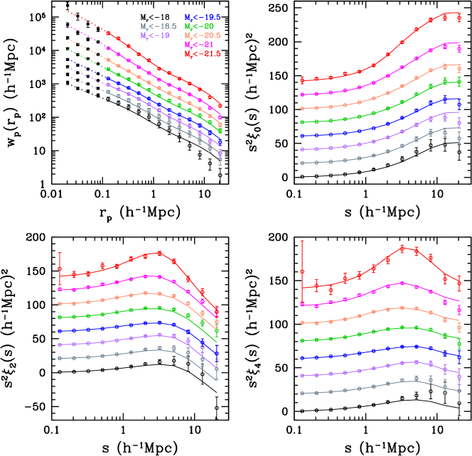
Figure 3: HOD fittings to the four sets of 2PCF measurements in Fig. 2. The measurements from the data are shown by open circles, while the HOD model fits are displayed as lines. For clarity, the measurements of different luminosity threshold samples are separated by $0.2{\rm dex}$ (for $w_{p}$) or $20(\,h^{-1}{\rm{Mpc}})^{2}$ (for $s^{2}\xi_{0,2,4}$) per sample, starting from the $M_{r}<-18$ sample. In the top left panel of $w_{p}(r_{p})$, the measurements at $r_{p}<0.1\,h^{-1}{\rm{Mpc}}$ (below the fibre-collision scale) are also shown, which are not included in the HOD fittings, while the dashed lines are the predictions from the best-fitting HOD models.

4.1 Fitting Results and the Mean Occupation Function

Fig. 3 shows the measurements and best-fitting HOD models for the four sets of 2PCFs as in Fig. 2. For clarify, offsets are applied to both the data points and bestfitting curves, $0.2{\rm dex}$ for $w_{p}$ and $20(\,h^{-1}{\rm{Mpc}})^{2}$ for $s^{2}\xi_{0,2,4}$ for each galaxy sample. As is evident, our HOD model leads to remarkably good fits to all the luminosity threshold samples, for both the projected and redshift-space 2PCFs. We choose to fit 2PCFs on scales above $0.1\,h^{-1}{\rm{Mpc}}$ to reduce any possible systematic effect in the fibre-collision correction (which is small according to Guo et al. 2012). With our bestfitting HOD model, we can predict the 2PCFs on smaller scales. The dotted curves and the filled circles in the top left panel of Fig. 3 show the prediction and the measurements on scales below $0.1\,h^{-1}{\rm{Mpc}}$. The best-fitting models reproduce well the measurements for all luminosity threshold samples down to $r_{p}=0.02\,h^{-1}{\rm{Mpc}}$, suggesting both an accurate HOD model and a robust fibre-collision correction.

Table 2: Best-fitting HOD parameters and derived parameters for the luminosity threshold samples

$M_{r}^{\rm max}$	-18.0	-18.5	-19.0	-19.5	-20.0	-20.5	-21.0	-21.5
$\chi^{2}/{\rm dof}$	$31.02/42$	$34.77/42$	$31.52/42$	$32.29/42$	$32.17/42$	$46.24/42$	$44.38/42$	$39.16/42$
$\log M_{\rm min}$	$11.18\pm 0.14$	$11.38\pm 0.10$	$11.58\pm 0.09$	$11.67\pm 0.07$	$11.95\pm 0.06$	$12.23\pm 0.04$	$12.78\pm 0.11$	$13.53\pm 0.10$
$\sigma_{\log M}$	$0.09\pm 0.49$	$0.23\pm 0.22$	$0.00\pm 0.21$	$0.01\pm 0.21$	$0.16\pm 0.17$	$0.18\pm 0.13$	$0.49\pm 0.13$	$0.72\pm 0.08$
$\log M_{0}$	$11.57\pm 0.24$	$11.73\pm 0.16$	$11.61\pm 0.22$	$11.80\pm 0.13$	$12.10\pm 0.10$	$12.42\pm 0.12$	$12.59\pm 1.59$	$13.13\pm 2.88$
$\log M_{1}^{\prime}$	$12.48\pm 0.12$	$12.71\pm 0.10$	$13.04\pm 0.08$	$13.07\pm 0.06$	$13.33\pm 0.06$	$13.57\pm 0.05$	$13.99\pm 0.07$	$14.52\pm 0.06$
$\alpha$	$0.97\pm 0.07$	$1.02\pm 0.06$	$1.12\pm 0.04$	$1.06\pm 0.03$	$1.08\pm 0.03$	$1.06\pm 0.05$	$1.14\pm 0.08$	$1.14\pm 0.16$
$\alpha_{c}$	$0.01\pm 0.13$	$0.01\pm 0.09$	$0.29\pm 0.12$	$0.28\pm 0.07$	$0.25\pm 0.07$	$0.29\pm 0.04$	$0.27\pm 0.04$	$0.31\pm 0.04$
$\alpha_{s}$	$0.95\pm 0.05$	$0.81\pm 0.04$	$0.77\pm 0.03$	$0.86\pm 0.03$	$0.84\pm 0.03$	$0.85\pm 0.03$	$0.97\pm 0.05$	$1.05\pm 0.08$
$\log M_{1}$	$12.53\pm 0.10$	$12.76\pm 0.09$	$13.06\pm 0.07$	$13.10\pm 0.05$	$13.35\pm 0.05$	$13.60\pm 0.04$	$14.01\pm 0.06$	$14.55\pm 0.06$
$f_{\rm{sat}}$	$26.87\pm 1.53$	$23.90\pm 1.20$	$20.74\pm 1.03$	$20.45\pm 0.80$	$17.87\pm 0.75$	$15.67\pm 0.57$	$12.46\pm 0.90$	$7.74\pm 0.74$
$\sigma_{c}$	$0.08\pm 8.39$	$0.37\pm 6.15$	$22.36\pm 9.81$	$22.85\pm 4.17$	$25.21\pm 7.17$	$35.05\pm 5.13$	$50.24\pm 7.95$	$99.20\pm 15.19$
$\sigma_{s}$	$146.24\pm 13.68$	$146.78\pm 12.80$	$173.85\pm 11.53$	$197.32\pm 9.01$	$234.58\pm 11.83$	$285.16\pm 13.91$	$442.16\pm 31.99$	$705.10\pm 70.42$

The halo mass is in units of $\,h^{-1}{\rm M_{\sun}}$. The best-fitting $\chi^{2}$ per degrees of freedom (dof) of the HOD modelling is also given. The degree of freedom of each sample is calculated as ${\rm dof}=N_{\rm 2PCF}+1-N_{\rm par}$, where the total number of data points ($N_{\rm 2PCF}+1$) is 49 (12 for each of $w_{p}$ and $\xi_{0,2,4}$, plus one number density constraint), and $N_{\rm par}=7$ is the number of HOD parameters. The derived parameter $\log M_{1}$ is the mass of a halo that on average hosts one satellite galaxy. The satellite fraction $f_{\rm{sat}}$ is in units of $\rm{per\,cent}$. The $\sigma_{c}$ and $\sigma_{s}$ (in units of $\,{\rm{km\,s^{-1}}}$) are the typical velocity dispersion of central and satellite galaxies, respectively (see details in text).

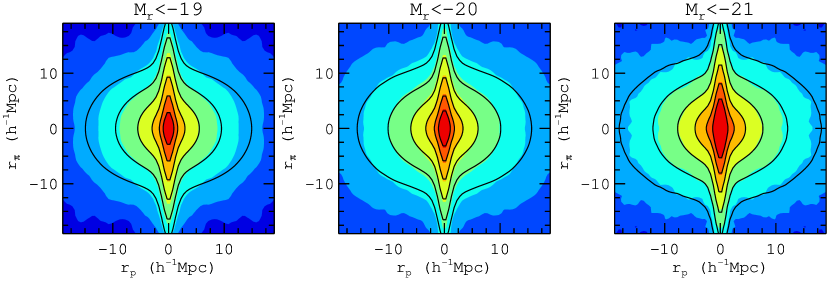
Figure 4: Comparisons between the measured redshift-space 3D 2PCF $\xi(r_{p},r_{\pi})$ (color scales) and the prediction from the best-fitting HOD model (black solid curves), for three representative luminosity-threshold samples. The data and models have the same contour levels of 0.3, 0.5, 1,2, 5, 10, and 20.

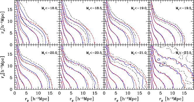
Figure 5: Comparisons between the predicted 3D 2PCF $\xi(r_{p},r_{\pi})$ from the best-fitting HOD models (red dotted curves) and the measurements (blue solid curves) for different luminosity-threshold samples. Contour levels are set to $\xi(r_{p},r_{\pi})=[0.3,0.5,1,2,5,10,20]$. The black dotted curves in each panel are contours at the level of $\xi(r_{p},r_{\pi})=0.3$ with $\xi(r_{p},r_{\pi})$ shifting by $\pm 1\sigma$ measurement error. The measurements of $\xi(r_{p},r_{\pi})$ in each panel (as well as the model curves) are smoothed with a Gaussian kernel to reduce the noise on large scales.

The best-fitting HOD parameters are listed in Table 2 for the different luminosity threshold samples. The $\chi^{2}/\rm{dof}$ of the fittings confirm the adequacy of the model in fitting the data. The derived parameters $M_{1}$ and $f_{\rm sat}$ are also displayed, together with the characteristic central and satellite galaxy velocity dispersions $\sigma_{c}=\alpha_{c}\sigma_{v}(M_{\rm min})$ and $\sigma_{s}=\alpha_{s}\sigma_{v}(M_{1})$ (see § 4.2 for more details).

In our modelling, we choose to fit the projected 2PCF and the redshift-space 2PCF multipole $\xi_{0,2,4}$, not the 3D redshift-space 2PCF $\xi(r_{p},r_{\pi})$ directly. The reason is the large dimension of $\xi(r_{p},r_{\pi})$ (e.g. 240 data points per sample for 12 $r_{p}$ bins and 20 $r_{\pi}$ bins), which makes it difficult to estimate a robust covariance matrix. However, with the best-fitting models, we can predict $\xi(r_{p},r_{\pi})$ and compare to the measurements as a cross-check. Such a comparison is shown in Fig. 4 for three representative luminosity-threshold samples of $M_{r}<-19$, $-20$ and $-21$. Two main RSD effects show up in $\xi(r_{p},r_{\pi})$. On large scales, the galaxy infall towards overdense regions as well as the streaming of galaxies out of underdense regions compresses the contours along the LOS direction, known as the Kaiser squashing effect (Kaiser, 1987; Hamilton, 1992). On small scales, the random motions of galaxies in virialized structures cause the $\xi(r_{p},r_{\pi})$ contours to appear stretched along the LOS direction, causing the FOG effect (Jackson, 1972; Huchra, 1988). The best-fitting HOD models reproduce the two features and the overall $\xi(r_{p},r_{\pi})$ measurements very well. In particular, the agreement between the measured and predicted 3D 2PCFs on small scales is remarkably good.

On large scales, there appears to be slight deviations of the predictions from the measurements. which are not significant, given the measurement errors. To see this and to have a comparison for all samples, in Fig. 5 we compare the 3D 2PCF contours for both the best-fitting predictions (red dotted curves) and the meausurements (blue solid curves). To illustrate the uncertainties on the measurements of $\xi(r_{p},r_{\pi})$, we show in each panel with black dotted curves the contours from $\pm 1\sigma$ of the $\xi(r_{p},r_{\pi})$ measurements for the outmost level ($\xi(r_{p},r_{\pi})=0.3$). The model fits of the $M_{r}<-18.5$ and $M_{r}<-19$ samples seem to be out of the 1$\sigma$ range of the measurements on large scales of $r_{p}>10\,h^{-1}{\rm{Mpc}}$, which is consistent with the over-prediction of the model on large scales, as seen in $w_{p}$ and $\xi_{0}$ in Fig. 3. However, such deviations are not significant given the highly correlated covariance matrix elements on these scales. The largest difference in the FoG feature is seen in the $M_{r}<-18.0$ sample, which is in fact not significant given the large error bars in the measurement for this sample. Overall the model successfully reproduces the luminosity dependent $\xi(r_{p},r_{\pi})$ measurements. As will be discussed in § 4.2, velocity bias is needed for the model to fit the redshift-space clustering.

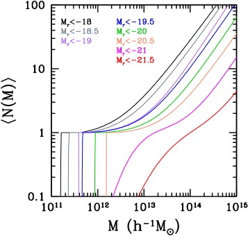
Figure 6: Mean halo occupation functions of the best-fitting models for different luminosity threshold samples.

The mean halo occupation functions for the different luminosity threshold galaxy samples are presented in Fig. 6. The most significant trend is that the host halo mass scale increases with the galaxy luminosity, as expected from HOD modelling of projected 2PCF $w_{p}(r_{p})$ from the same SDSS data by Zehavi et al. (2011) (see also Zehavi et al. 2005; Zheng et al. 2007). Compared to the HOD model used in Zehavi et al. (2011), our model in this paper adopts different cosmological parameters and halo definition. Furthermore, we shift to a simulation-based model, rather than an analytic model. Finally, we jointly fit the projected 2PCF $w_{p}$ and the redshift-space 2PCFs $\xi_{0,2,4}$, while Zehavi et al. (2011) only fit $w_{p}$. Accounting for these differences, our results are in good agreement with those in Zehavi et al. (2011). We note that the uncertainties in many HOD parameters (and the derived satellite fraction) from the modelling in this paper appear to be larger than those in Zehavi et al. (2011) from modelling $w_{p}$ only. This can be attributed to the differences in the models. The accuracy of the measured small-scale data points exceed that of the analytic HOD model used in Zehavi et al. (2011), which may be the reason of their large $\chi^{2}/$dof (2–3 for some cases). As a consequence, the uncertainties in the HOD parameters can be artificially underestimated. The simulation-based model used in this paper is a more accurate model, leading to good values of $\chi^{2}/$dof and improved error estimates in the parameters.

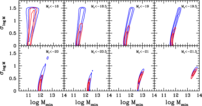
Figure 7: Comparisons between the constraints on the HOD parameters $M_{\rm min}$ and $\sigma_{\log M}$ from fitting $w_{p}$ (blue contours) and jointly fitting $w_{p}$ and $\xi_{0,2,4}$ (red contours).

We also perform $w_{p}$-only fit with the simulation-based model and compare to the results from fitting both $w_{p}$ and $\xi_{0,2,4}$. We find that redshift-space 2PCFs help tighten the constraints on the HOD parameters. As an example, we show in Fig. 7 the comparison of the constraints on $M_{\rm min}$ and $\sigma_{\log M}$ from fitting $w_{p}$ only (blue contours) and jointly fitting $w_{p}$ and $\xi_{0,2,4}$ (red contours). We set a prior of $\sigma_{\log M}<1.5$ when fitting the data to have a reasonable value of the scatter. Clearly, a substantial improvement with the redshift-space 2PCFs is to narrow down the range of $\sigma_{\log M}$, especially for less luminous samples (with the $M_{r}<-18$ as an exception, which has a tighter $M_{\rm min}$).

Even though redshift-space 2PCFs help tighten the constraints on $\sigma_{\log M}$, we note that for faint galaxy samples the cutoff profile in the mean central occupation function is still not well constrained, as indicated by the large errors (Table 2 and Fig. 7). It is consistent with a sharp cutoff at $M_{\rm min}$, and in Fig. 6 we choose to plot the best-fitting models with $\sigma_{\log M}\simeq 0$ for these samples. The constraints on $M_{\rm min}$ and $\sigma_{\log M}$ mainly come from the galaxy bias (large scale 2PCF amplitude) and the galaxy number density. The galaxy bias is mainly determined by haloes around $M_{\rm min}$. For faint samples, $M_{\rm min}$ is in the range that halo bias is insensitive to halo mass. As a consequence, the galaxy bias is insensitive to the way of populating galaxies into haloes of different masses around $M_{\rm min}$, i.e. insensitive to the change in $\sigma_{\log M}$. A change in $\sigma_{\log M}$ can be easily compensated by a slight change in $M_{\rm min}$ to maintain the galaxy number density. Therefore, the cutoff profiles for faint samples are not well constrained. Conversely, $\sigma_{\log M}$ is much better constrained for the luminous samples as a result of the steep dependence of halo bias and halo mass function on halo mass toward the high-mass end.

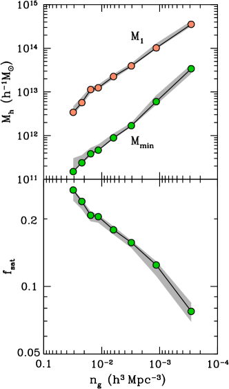
Figure 8: Top: characteristic mass scales ($M_{\rm min}$ and $M_{1}$) of haloes hosting central galaxies and satellites as a function of the sample number density $n_{g}$. Bottom: satellite fraction as a function of the sample number density. The shaded area around each curve shows the $1\sigma$ uncertainties in the parameter.

Fig. 8 shows the dependence of the characteristic mass scales ($M_{\rm min}$ for central galaxies and $M_{1}$ for satellite galaxies) and the satellite fraction $f_{\rm sat}$ on the sample number density $n_{g}$. The dependence of any of those parameters on $n_{g}$ roughly follows a power-law form. As pointed out in Guo et al. (2014), the dependence of $M_{\rm min}$ on the number density largely comes from the nearly power-law form of the halo mass function over a large mass range. The mass $M_{\rm min}$ is mostly determined by matching the halo number density with the galaxy number density, modulated by $\sigma_{\log M}$. There is a trend that the ratio $M_{1}/M_{\rm min}$ decreases as the sample number density decreases (or the sample luminosity increases), consistent with those found in literature (e.g. Zehavi et al., 2005; Skibba et al., 2007; Zheng et al., 2009; Zehavi et al., 2011; Guo et al., 2014; McCracken et al., 2015; Skibba et al., 2015). This is a manifestation of the halo mass dependent competition between accretion of galaxies into haloes and destruction of galaxies inside haloes. From the bottom panel of Fig. 8, we see that fainter galaxies are more likely to be satellite galaxies in massive haloes. The satellite fraction follows $f_{\rm sat}\simeq 0.1[\bar{n}_{g}/(10^{-3}h^{3}{\rm Mpc}^{-3})]^{1/3}$, as also shown in other surveys (Guo et al., 2014), which can be used to estimate the satellite fraction given the number density of a threshold galaxy sample. Note that the values of satellite fraction are slightly lower than those inferred in Zehavi et al. (2011), which can be mostly attributed to the difference in the definitions (hence the sizes) of haloes.

4.2 Galaxy Velocity Bias

The constraints on the galaxy velocity bias parameters are shown in Fig. 9, including the 68 per cent and 98 per cent contours in the $\alpha_{c}$–$\alpha_{s}$ plane and the marginalized distributions of $\alpha_{c}$ and $\alpha_{s}$ for each sample. In terms of the tightness in the central galaxy velocity bias $\alpha_{c}$ constraints, the luminous and faint samples show a dichotomy.

For the luminous samples (more luminous than $M_{r}=-19.5$), both the central and satellite velocity bias parameters are well constrained, as shown in the top left panel. The case without any galaxy velocity bias (i.e. $\alpha_{c}=0$ and $\alpha_{s}=1$) is far beyond the 95 per cent contours of all luminous samples. That is, galaxy velocity bias is required to reproduce the redshift-space clustering in the local universe for luminous samples.

The central velocity bias parameter $\alpha_{c}$ for luminous samples is about 0.3 (top-left and bottom-left panels in Fig. 9). It shows no significant dependence on galaxy luminosity. The existence of the central velocity bias implies that these luminous central galaxies are not at rest at the halo centres with respect to the bulk motion of the haloes. This reflects the mutual (non)relaxation status of central galaxies and host haloes, which are related to the merger history of the galaxies and the formation history of haloes (see more detailed discussions in G15). The value of $\alpha_{c}$ inferred from our modelling of the redshift-space clustering is in agreement with the estimates from galaxy group catalogues in the SDSS (e.g. van den Bosch et al., 2005), which uses the mean velocity of satellites as a proxy for the halo velocity.

The constraints on the central velocity bias parameter $\alpha_{c}$ are loose for the three faint samples (with threshold luminosity fainter than $M_{r}=-19.0$), as seen from the contours in the top-right panel and the corresponding curves in the bottom-left panel of Fig. 9. For the $M_{r}<-19$ sample, $\alpha_{c}$ is different from zero only at the 2.5$\sigma$ level (see Table 2). For the other two fainter samples, $\alpha_{c}$ is consistent with zero. The loose constraints can be partly attributed to the relatively large uncertainty in the clustering measurements and in the jackknife covariance matrix estimate for the faint samples, as the sample volumes are substantially smaller than those of the luminous samples (see Fig. 1 and Table 1), especially on large scales where $\alpha_{c}$ is mostly constrained (see Fig.6 of G15). The three faint samples have volumes that are 10%, 24%, and 43% that of the $M_{r}<-19.5$ sample, which has the smallest volume among the luminous samples. The other possible cause of the loose constraints can be the redshift errors. As the central velocity bias, in terms of velocity dispersion (see below), approaches or drops below the level of redshift errors (about 13 ${\rm km\,s^{-1}}$; see Appendix A), the sensitivity of RSD to the central velocity bias is reduced, likely the case for the faint samples.

For the satellite velocity bias, all samples show good constraints. Sample volume becomes less important here, since the constraints mainly come from the small-scale FoG effect (see Fig.6 of G15), where the uncertainties in the measurements are small. However, the faintest sample ($M_{r}<-18$) may still be affected by the small sample size and the noisy covariance matrix estimate, and we should interpret the satellite velocity bias with caution. If we neglect the $M_{r}<-18$ sample, the satellite velocity bias $\alpha_{s}$ constraints show a more or less continuous trend with luminosity, i.e. higher values of $\alpha_{s}$ for more luminous sample. Probably more appropriately, the satellite velocity bias constraints can be divided into two groups. For the two most luminous samples (more luminous than $L_{*}$, corresponding to $M_{r}=-20.44$; Blanton et al. 2003b), $\alpha_{s}$ is consistent with unity. That is, the motion of the luminous satellites closely follows that of the dark matter. For samples with threshold luminosity fainter than $L_{*}$, $\alpha_{s}$ is about 0.8 – 0.85. That is, for those samples, satellites moves more slowly than dark matter particles.

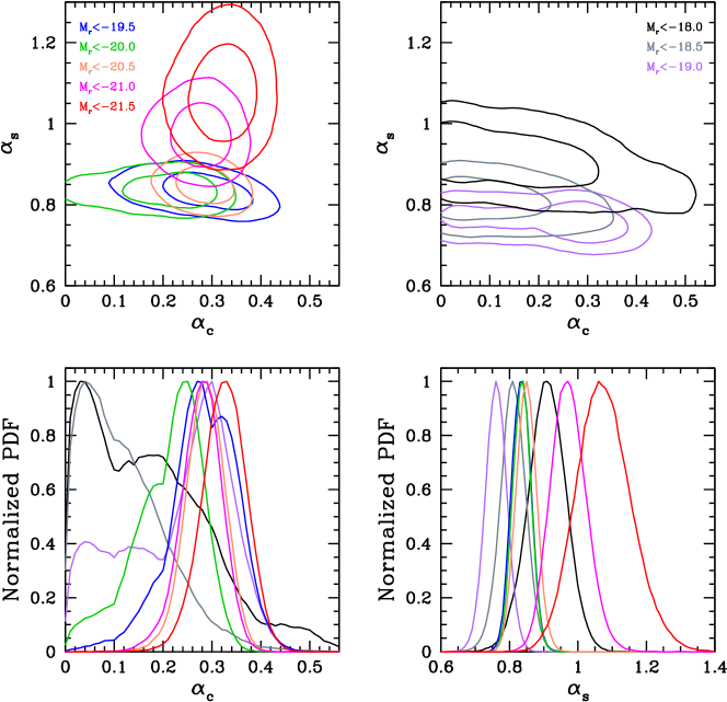
Figure 9: Top panels: marginalized probability distributions of central and satellite galaxy velocity bias parameters for the luminous (left) and faint (right) galaxy samples. The contours show the 68 and 95 per cent confidence levels for the two parameters. Bottom panels: 1D probability distribution of the central (left) and satellite (right) galaxy velocity bias parameters for various luminosity-threshold samples.

In a steady state, the spatial distribution and velocity distribution of satellite galaxies inside haloes are related to each other. In our modelling, we draw random dark matter particles for the position of satellites. That is, we implicitly assumed that the spatial distribution of satellites follows that of the dark matter, which is well described by the Navarro-Frenk-White (NFW) profile (Navarro et al., 1997). For the two luminous samples, $\alpha_{s}$ is around unity, i.e., their satellite velocity distribution is consistent with that of the dark matter. Therefore, based on the constraints we infer, an NFW profile and associated velocity distribution for satellites are able to explain the redshift-space clustering for the luminous sample. More modelling efforts are needed to see whether other profiles and the corresponding velocity distributions are preferred or not (see the tests in G15). For the other, faint samples, the inferred $\alpha_{s}$ ($\sim$0.8 – 0.85) differs substantially from unity, inconsistent with the value for the NFW profile. The result alone suggests that the spatial distribution of faint satellites should deviate from the NFW profile. Our current model, however, is not able to provide more information on how significant a deviation it needs to be. For an improved model, one can consider to parameterize the spatial profile of satellites and solve for the corresponding velocity distribution in a self-consistent manner, which is beyond the scope of this paper.

Watson et al. (2010) and Watson et al. (2012) analyzed the small-scale (down to ${\sim}0.01\,h^{-1}{\rm{Mpc}}$) clustering ($w_{p}$) of the SDSS Main galaxy sample and luminous red galaxies. They found that the spatial distribution of faint satellite galaxies (below $M_{r}=-20$) is consistent with the NFW profile, while that of bright satellite galaxies deviates from the NFW profile (with a steeper inner profile). These seem opposite to what we find from modelling the redshift-space clustering. An improved model is necessary to constrain the range of profiles allowed by the redshift-space clustering data and to see whether this apparent difference is significant.

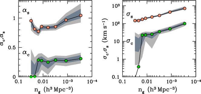
Figure 10: Velocity bias and typical velocity dispersion. Left: central and satellite galaxy velocity bias as a function of the sample number density $n_{g}$. Right: dependence of the typical central and satellite galaxy velocity dispersions, $\sigma_{c}$ and $\sigma_{s}$, on the sample number density. The shaded area show the 68 per cent and 95 per cent confidence levels of the parameters. The solid lines with circles are the best-fitting models.

In the left panel of Fig. 10, we summarize the constraints on the velocity bias parameters $\alpha_{c}$ and $\alpha_{s}$ as a function of galaxy number density (more luminous galaxy samples have lower number densities). For galaxies $M_{r}<-19.5$ and brighter, there is no significant dependence of $\alpha_{c}$ on number density. The three faint galaxy samples (with the highest number densities) seem to have lower values of $\alpha_{c}$, consistent with zero, but with large error bars. Since the host halo mass increases as the galaxy luminosity increases (or as the number density decreases), the trend also indicates the weak dependence of $\alpha_{c}$ on the host halo mass. With the faintest sample excluded (smallest sample volume), the dependence of satellite velocity bias $\alpha_{s}$ on the luminosity for faint galaxies is also weak, while $\alpha_{s}$ shows a clear increase with luminosity for $M_{r}<-21$.

To interpret the velocity bias results, the more meaningful physical quantities are the velocity dispersions of central and satellite galaxies inside haloes, denoted as $\sigma_{c}$ and $\sigma_{s}$, respectively. Given the velocity bias parameters, velocity dispersions depend on halo mass, and we choose to evaluate typical values in representative haloes. For central galaxies, the velocity bias constraint is mainly contributed from haloes around $M_{\rm min}$, and we compute the typical central galaxy velocity dispersion as $\sigma_{c}=\alpha_{c}\sigma_{v}(M_{\rm min})$. For satellite galaxies, the effect of the velocity bias on clustering comes from haloes around $M_{1}$, and the typical satellite velocity dispersion is computed as $\sigma_{s}=\alpha_{s}\sigma_{v}(M_{1})$. The right panel of Fig. 10 shows the dependencies of these typical velocity dispersions on sample number density, which roughly follow power-law relations, $\sigma_{c}\simeq 55\,{\rm{km\,s^{-1}}}[\bar{n}_{g}/(10^{-3}h^{3}{\rm Mpc}^{-3})]^{-0.45}$ and $\sigma_{s}\simeq 437\,{\rm{km\,s^{-1}}}[\bar{n}_{g}/(10^{-3}h^{3}{\rm Mpc}^{-3})]^{-1/3}$.

The existence of galaxy velocity bias reflects the dynamical evolution of galaxies inside haloes. For example, infalling satellites experience tidal striping and dynamical friction in the dark matter haloes, affecting its velocity distribution. For central galaxies, the existence of velocity bias indicates that central galaxy and the host haloes are not mutually relaxed. A likely cause can be the halo mergers and the subsequent galaxy mergers. Our results can be used to assess the dependence of the degree of relaxation after mergers on halo mass (or galaxy number density). For mergers of haloes of similar mass, the mean pairwise infall velocity $v_{12}$ on large scales is proportional to the bias factor (Sheth et al., 2001; Zhang & Jing, 2004). With the luminosity-dependent bias factor in Zehavi et al. (2011), we find that the bias factor approximately scales as $n_{g}^{-0.11}$, which means that the pairwise infall velocity $v_{12}\propto n_{g}^{-0.11}$ before merger. The central velocity dispersion constrained from the RSD ($\alpha_{c}\propto n_{g}^{-0.45}$) is much steeper than the infall velocity. We therefore conclude that central galaxies in lower mass haloes are more relaxed with respect to the host haloes, compared with their counterparts in more massive haloes, consistent with an overall earlier formation and thus more time for relaxation of the lower mass haloes.

4.3 Dependence of Velocity Bias on Cosmology ($\Omega_{m}$)

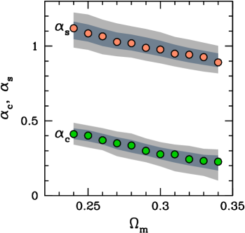
Figure 11: Dependence of central and satellite galaxy velocity bias on the cosmological parameter $\Omega_{m}$. The central and satellite velocity bias are displayed in circles of different colours. The shaded area show the 68 and 95 per cent confidence levels of the parameters.

The velocity bias constraints we infer rely on the MultiDark simulation with the assumed cosmology. The cosmological parameters are close to the results from Planck (Planck Collaboration et al., 2014). It is useful to see whether the velocity bias constraints are robust against reasonable change in cosmology. Here, we limit our investigation to the change in $\Omega_{m}$. Instead of using simulations with different $\Omega_{m}$ parameters, we use the appropriate scaling relations with the MDPL simulation for the corresponding change in the dark matter halo properties when varying $\Omega_{m}$.

According to Zheng et al. (2002) and Tinker et al. (2006), if two simulations have the identical initial matter fluctuation spectrum (including amplitude and phase) but different values of $\Omega_{m}$, there exists a simple relation between simulation outputs at a given linear growth factor $G$. There are correspondences between haloes in the two simulations, and the corresponding haloes have the same radius with the mass scaling with $\Omega_{m}$. Halo velocity scales with the growth rate $f\equiv d\ln G/d\ln a$, with $a$ the scale factor. The internal velocity dispersion inside haloes scales with $\Omega_{m}^{0.5}$. We therefore modify our default simulation output by scaling the halo mass $M$, halo velocity $v_{h}$, dark matter particle velocity $v_{p}$, and the 1D velocity dispersion $\sigma_{v}$ of dark matter particles in haloes in the following way,

$$M = \left(\Omega_{m}/\Omega_{m,0}\right)M_{0},$$ (9)

$$v_{h} = \left(f/f_{0}\right)v_{h,0},$$ (10)

$$v_{p}-v_{h} = \left(\Omega_{m}/\Omega_{m,0}\right)^{1/2}(v_{p,0}-v_{h,0}),$$ (11)

$$\sigma_{v} = \left(\Omega_{m}/\Omega_{m,0}\right)^{1/2}\sigma_{v,0},$$ (12)

where the symbols with subscript ‘0’ denote the values in the fiducial MDPL simulation. The halo mass function also changes accordingly in each scaled simulation. We build eleven scaled simulation catalogues, varying $\Omega_{m}$ from $0.24$ to $0.34$ with a step of $\Delta\Omega_{m}=0.01$. We then apply our HOD model to the $M_{r}<-21$ sample based on the eight scaled simulations to constrain the velocity bias parameters.

We show in Fig. 11 the dependence of the velocity bias parameter constraints on $\Omega_{m}$. Both the central and satellite velocity biases decrease with increasing $\Omega_{m}$, as expected. Increasing $\Omega_{m}$ leads to higher halo-halo and internal halo velocity dispersions, and the velocity bias parameters decrease to compensate such a change to match the redshift-space clustering. For the range of $\Omega_{m}$ considered here, both velocity bias parameters are well constrained. In particular, the central velocity bias differs from zero for all the cases, which shows that our constraints are robust against reasonable changes in cosmology.

We note that the luminosity-threshold samples used in this paper are constructed over different redshift ranges according to the range for which they are volume limited (see Fig. 1 and Table 1). If we were to apply the cosmology change and compare the results among different samples, the difference in the sample mean redshifts needs to be accounted for, which leads to small effective cosmology changes. As mentioned in § 3, our test with the model built on the $z=0.1$ simulation output shows that the inferred HOD parameters are within the uncertainties of those from the default model built on the $z=0$ output. So the effect of cosmology change from the difference in mean redshift is small. Furthermore, here we only focus on one sample and aim to see the sensitivity of velocity bias constraints to cosmology, and the effective cosmology change among different samples becomes irrelevant. With one sample, there is another effect related to the cosmology change. In principle, when varying the cosmological parameter $\Omega_{m}$, we need to rescale or remeasure the 3D 2PCFs and then perform the modelling. Otherwise, the Alcock-Paczynski effect (Alcock & Paczynski, 1979) would introduce an additional distortion in the 2PCFs. However, since the galaxy samples are local, with $z\sim 0$, the comoving distance is insensitive to $\Omega_{m}$ and the effect is tiny. For example, at the mean redshift of the $M_{r}<-21$ sample, $z\sim 0.12$, the comoving distance changes by less than 1% in the whole range of $\Omega_{m}$ we study here, which has little effect on the 2PCF measurements. We therefore do not rescale or remeasure the 2PCFs changing the cosmology.

Relevant to the RSD effect, a more interesting change in cosmology is in the combination of the growth rate and fluctuation amplitude, $f\sigma_{8}$. Because of the high precision measurements, the small-scale redshift-space clustering can help tighten the constraints on $f\sigma_{8}$ (e.g. Reid et al., 2014), providing potentially stringent tests to the $\Lambda$CDM cosmology and theory of gravity. We reserve such an investigation on the $f\sigma_{8}$ constraints with the SDSS Main galaxies for a future work.

5 Summary and Discussions

We measure the projected and redshift-space 2PCFs for volume-limited, luminosity-threshold samples of SDSS Main galaxies, on small to intermediate scales ($0.1$–$25\,h^{-1}{\rm{Mpc}}$). The measurements are interpreted within the HOD framework to infer the relation between galaxies and dark matter haloes. In particular, the RSD effects in the redshift-space 2PCFs enable us to constrain the kinematics of central and satellite galaxies inside dark matter haloes and infer the difference between the motions of galaxies and dark matter.

It is the first time that the redshift-space clustering of local galaxies is accurately measured on scales as small as $\sim$$0.1\,h^{-1}{\rm{Mpc}}$. The measurements become possible with the accurate fibre-collision correction method developed in Guo, Zehavi & Zheng (2012), which makes use of the resolved collided galaxy pairs in tile overlap regions to recover the small scale clustering. Previous measurements (e.g. Hawkins et al., 2003; Zehavi et al., 2005) rely on either angular or nearest neighbour fibre-collision corrections, which results in systematics at the level of the data precision (Guo et al., 2012). With our measurements, we find that both the projected and redshift-space 2PCFs show a clear dependence on galaxy luminosity, generally with a higher clustering amplitude for more luminous galaxies on both small and large scales. The dependence on luminosity becomes stronger for galaxies above $\sim$$L_{*}$. The overall trend is consistent with previous results based on the projected 2PCFs (e.g. Zehavi et al., 2011).

To interpret the measurements, similar to G15, we resort to an accurate HOD model based on a high-resolution $N$-body simulation. In addition to the mean halo occupation function, the model also parameterizes the central and satellite galaxy velocity bias. For the first time, a halo-based model is applied to model the measured luminosity dependent small- and intermediate-scale redshift-space clustering of local galaxies. Previous studies usually focus on relatively large scales and adopt a streaming model (e.g. Peacock et al., 2001; Hawkins et al., 2003; Bel et al., 2014; Howlett et al., 2015). The commonly inferred quantities include the linear redshift distortion parameter and the mean pairwise velocity dispersion of galaxies (e.g Cabré & Gaztañaga, 2009) or its scale dependence (e.g. Li et al., 2007). Our halo-based model, as applied in G15 (see Reid et al. 2014 for a similar model), makes use of the kinematic information of haloes and parameterizes the galaxy velocity distribution on top of it, rather than an overall mean velocity dispersion. It allows us to constrain the occupation and kinematic distribution of galaxies at the level of dark matter haloes, a more informative extraction from galaxy redshift-space clustering data. We find that the model is able to successfully reproduce the observed projected 2PCF $w_{p}(r_{p})$, the redshift-space multipole moments $\xi_{0}(s)$, $\xi_{2}(s)$ and $\xi_{4}(s)$, and the 3D 2PCF $\xi(r_{p},r_{\pi})$, on all scales for all SDSS luminosity-threshold samples (Fig. 3 and Fig. 5).

Consistent with previous work that only model the projected 2PCF (e.g. Zheng et al., 2007; Zehavi et al., 2011), we find that the clustering trend with luminosity can be explained by the fact that more luminous galaxies reside in more massive haloes. The characteristic halo masses, $M_{\rm min}$ (for central galaxies) and $M_{1}$ (for satellite galaxies), increase with increasing luminosity threshold. The satellite fraction, $f_{\rm sat}$, drops as the luminosity threshold increases. The dependence of $M_{\rm min}$, $M_{1}$, and $f_{\rm sat}$ on the sample number density (which is directly related to the sample luminosity threshold) can be well described by power-law relations. Compared to the $w_{p}$-only modelling results, the redshift-space 2PCFs help tighten the constraints on the HOD parameters. However, we find that for the faint galaxy samples (with luminosity threshold below $L_{*}$), the cutoff profile (characterized by the parameter $\sigma_{\log M}$) in the mean occupation function of central galaxies is still loosely constrained.

Besides the above results, the brand-new outcomes from our modelling are the constraints on galaxy kinematics inside haloes, coming from the RSD effects on both small and large scales. The redshift-space clustering data require the existence of a non-zero central galaxy velocity bias of about $0.3$ for luminous samples (with threshold luminosity $M_{r}<-19.5$), while for faint samples the central velocity bias parameters are loosely constrained but consistent with the above value. That is, in the rest-frame (centre-of-mass frame) of a halo, the central galaxy on average moves at a speed about 30% that of dark matter particles. The central galaxy velocity bias in our model is in agreement with the estimates from the galaxy group catalogues in the SDSS (e.g. van den Bosch et al., 2005). This mutual non-relaxation between central galaxies and dark matter haloes can result from mergers and dynamical evolution of galaxies and haloes. Converting the value to physical speed and comparing to the typical infall velocity before merging, our results imply that galaxies in lower mass haloes are more relaxed with respect to the host haloes, consistent with their earlier formation time. Further theoretical investigation of such an evolution paradigm using high-resolution cosmological hydrodynamic galaxy formation simulations will be pursued in future work.

For satellite galaxies, we find that the two most luminous samples have satellite velocity bias consistent with unity, which means that they follow closely the motion of dark matter. The satellite velocity bias $\alpha_{s}\sim 0.85$ for fainter samples implies that fainter satellites move more slowly than dark matter. If satellite motion is in a steady state, the result suggests that the spatial distribution profile of faint satellites should differ from that of dark matter. More informative constraints need an improved model that allow for a self-consistent treatment of the spatial and kinematic distributions of satellites, which would also lead to tighter constraints than using only projected spatial clustering measurements (e.g. Watson et al., 2012; Wang et al., 2014b). An improved model can also include the effect of halo assembly bias to see its influence on the HOD (e.g. Zentner et al. 2014; but see Lin et al. 2015) and velocity bias. The existence of satellite galaxy velocity bias affects any dynamical inference based on satellite velocity dispersions. For example, the effect needs to be taken into account when using the velocity dispersion of the galaxy cluster members to estimate the halo mass of galaxy clusters (Goto et al., 2003; Old et al., 2013).

In G15, velocity bias is inferred for a sample of $z\sim 0.5$ luminous galaxies ($n_{g}=2.19\times 10^{-4}h^{3}{\rm Mpc}^{-3}$). Converted to the same velocity bias definition used in this paper (i.e. in the centre-of-mass frame of haloes), their result on the velocity dispersion for central galaxies in haloes of $\sim 10^{13.35}\,h^{-1}{\rm M_{\sun}}$ is about $96\pm 8\,{\rm km\,s^{-1}}$. On average, these haloes evolve to $\sim 10^{13.55}\,h^{-1}{\rm M_{\sun}}$ haloes at z$\sim 0$ (e.g. Zhao et al., 2009), around $M_{\rm min}$ of the $M_{r}<-21.5$ sample ($n_{g}=2.86\times 10^{-4}h^{3}{\rm Mpc}^{-3}$). We thus can have an approximate connection between the two samples at $z\sim 0.5$ and $z\sim 0$ from the halo evolution, following the same spirit as in Zheng et al. (2007), which is also supported by the number density comparison. The central galaxy velocity dispersion for the $M_{r}<-21.5$ is about $99\pm 15\,{\rm km\,s^{-1}}$. Such a preliminary analysis shows that the velocity dispersion for luminous central galaxies has not evolved much since $z\sim 0.5$ (in fact, it has marginally increased, but only at a $\sim 0.3\sigma$ level). We can assume a simple circular motion of the central galaxy in the inner NFW halo to study the implication of the result. With the $z\sim 0.5$ velocity bias result, the radius of the orbit can be inferred to be about 0.4% of the virial radius of the halo (G15). The corresponding dynamical friction time scale is estimated to be $\sim$0.1 Myr, much shorter than the 3.7 Gyr time span from $z\sim 0.5$ to $z\sim 0.1$. Therefore, a substantial central velocity bias at $z\sim 0$ indicates that these luminous central galaxies and their host haloes (or the cores of haloes and the rest of the haloes) may have been constantly disturbed by galaxy and halo mergers. We expect that velocity bias of galaxies inferred from different redshifts can help study the dynamical evolution of galaxies and haloes and test galaxy formation theory.

The galaxy peculiar velocity field is directly related to the growth of structures in the universe. RSD effects can be used to constrain cosmology, especially the growth rate (i.e. the $f\sigma_{8}$ parameter) to test the theory of gravity (e.g. Guzzo et al., 2008; Percival & White, 2009). The statistical power of small-scale RSD measurements have the potential to greatly tighten the constraints (e.g. Tinker et al., 2006; Tinker, 2007; Reid et al., 2014). The effect of velocity bias needs to be taken into account when using small-scale redshift-space clustering to constrain cosmology. We leave an investigation on cosmological applications based on our measurements and model for a future work.

Appendix A The Redshift Error Distribution

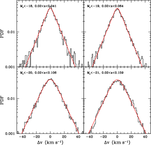
Figure 12: Redshift error distribution of SDSS Main galaxies with different luminosity thresholds. In each panel, the histogram is obtained from galaxies with repeat spectroscopic observations, and the red curve is the best-fitting Gaussian-convolved Laplace distribution. See the text.

In order to develop an accurate HOD model to apply to the redshift-space clustering measurements in SDSS, we need to carefully account for the distribution of redshift measurement errors of galaxies. The effect of redshift errors is to add apparent peculiar velocity dispersion to galaxies, which, if not accounted for, introduces apparent velocity bias component. This is especially important for faint galaxies, because the potentially small central and satellite velocities inside haloes make the constraints more vulnerable to redshift errors.

To properly investigate the redshift errors in the SDSS Main galaxies, we make use of all the galaxies with repeat spectra for each luminosity-threshold sample to derive the distribution of redshift measurement errors. In particular, for a galaxy with $n$ observations and hence $n$ redshift measurements, we construct the estimator of the velocity error in each measurement as

$$\Delta v_{i}=\sqrt{\frac{n}{n-1}}\frac{c(z_{i}-\bar{z})}{1+\bar{z}},$$ (13)

where $z_{i}$ is the $i$–th redshift measurement for this galaxy ($i=1,...,n$) and $\bar{z}$ is the mean of the $n$ measurements, and the factor $\sqrt{n/(n-1)}$ makes the estimator unbiased.

The histograms in Fig. 12 show the probability distribution of the redshift errors in terms of the peculiar velocity errors $\Delta v$ in four different luminosity-threshold samples. We find that the distribution has more extended tails than a naively assumed Gaussian distribution. The extended part follows closely the double exponential distribution or the Laplace distribution (appearing as straight lines in the plot), while the central part can be described by a Gaussian core (less sharply peaked than the Laplace distribution). In fact, the distribution can be remarkably fitted by a Gaussian-convolved Laplace distribution, shown as the red curves of Fig. 12. A random deviate $\Delta v$ for such a distribution can be obtained by the sum of two independent Gaussian and Laplace random numbers, i.e. $\Delta v=\Delta v_{\rm gau}+\Delta v_{\rm exp}$, with the distribution functions of $\Delta v_{\rm gau}$ and $\Delta v_{\rm exp}$ as

$$f_{\rm gau}(\Delta v_{\rm gau}) = \frac{1}{\sqrt{2\pi}\sigma_{\rm gau}}\exp\left(-\frac{\Delta v_{\rm gau}^{2}}{2\sigma_{\rm gau}^{2}}\right),$$ (14)

$$f_{\rm exp}(\Delta v_{\rm exp}) = \frac{1}{\sqrt{2}\sigma_{\rm exp}}\exp\left(-\frac{\sqrt{2}|\Delta v_{\rm exp}|}{\sigma_{\rm exp}}\right).$$ (15)

The parameters $\sigma_{\rm gau}$ and $\sigma_{\rm exp}$ are the standard deviations for the Gaussian and Laplace distributions, respectively.

Why does the redshift error follow more closely to a Laplace distribution than a Gaussian distribution? Laplace distribution can be thought as the distribution of Gaussian random variables with mean zero and stochastic variance that has an exponential distribution. We speculate that for a given galaxy, the redshift error follows a Gaussian distribution, but the variance of the distribution varies from galaxy to galaxy. We expect that for higher variance in redshift errors, there are fewer galaxies, and that there is a minimum variance (e.g. from the spectral resolution). With such an expectation, the probability distribution of the variance can be approximated as an exponential distribution with a cutoff towards lower value. The overall distribution of the redshift errors then follows a Laplace distribution with the central part modified by the lower cutoff on the variance. In such a scenario, the random variable $\Delta v$ can be obtained through the product of two independent random numbers, $\Delta v=\sigma u$, where $u$ follows the unit normal distribution and $\sigma^{2}$ follows a modified exponential distribution of scale parameter $\sigma_{e}^{2}$ with non-zero values above a threshold $\sigma_{t}^{2}$. The two parameters $\sigma_{e}$ and $\sigma_{t}$ characterize the tail and central part of the distribution. The above speculation is supported by the data. In Fig. 13, we show the histogram of the sample variance $s^{2}$ of the redshift error distribution estimated from galaxies with $n=2$ repeat spectra, with $s^{2}=\sum_{i=1}^{n}[c(z_{i}-\bar{z})/(1+\bar{z})]^{2}/(n-1)$ for each galaxy. The dotted curve shows an exponential distribution of the variance $\sigma^{2}$ of the Gaussian error distribution with $\sigma_{e}^{2}=200{\rm(km\,s^{-1})^{2}}$ and $\sigma_{t}^{2}=20{\rm(km\,s^{-1})^{2}}$. The expected distribution of sample variance $s^{2}$ is shown as the solid curve. It is derived from convolving the dotted curve with the sample variance distribution at given $\sigma^{2}$ [noting that $(n-1)s^{2}/\sigma^{2}$ follows a $\chi^{2}$ distribution with $n-1$ degrees of freedom]. Clearly, the $s^{2}$ distribution from galaxies with repeat spectra is consistent with being from a sample of Gaussian errors with stochastic variance that follows a truncated exponential distribution.

In this paper, we adopt the Gaussian-convolved Laplace distribution to model the redshift error distribution. From fitting the histograms of redshift errors with such a distribution for different luminosity-threshold galaxy samples, we derive the parameters $\sigma_{\rm gau}$ and $\sigma_{\rm exp}$. We find that it is sufficient to adopt two groups of parameters, for bright and faint galaxies, respectively. We use $\sigma_{\rm gau}=2\,{\rm{km\,s^{-1}}}$ and $\sigma_{\rm exp}=12.5\,{\rm{km\,s^{-1}}}$ for the luminosity threshold samples of $M_{r}<-18$, $-18.5$ and $-19$, while the more luminous samples have $\sigma_{\rm gau}=5\,{\rm{km\,s^{-1}}}$ and $\sigma_{\rm exp}=14.5\,{\rm{km\,s^{-1}}}$. We incorporate the redshift errors into our model by adding shifts in the redshift-space positions of galaxies, following the corresponding Gaussian-convolved Laplace distribution.

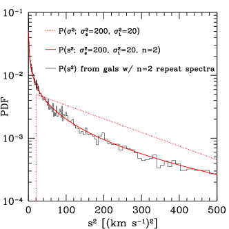
Figure 13: Distribution of sample variance $s^{2}$ of redshift errors. For each galaxy with $n=2$ repeat spectra, the sample variance $s^{2}$ is computed as $s^{2}=\sum_{i=1}^{n}[c(z_{i}-\bar{z})/(1+\bar{z})]^{2}/(n-1)$. The distribution is consistent with the expected $s^{2}$ distribution (solid curve) for the following case: the redshift error of each galaxies follows a Gaussian distribution, while the variance $\sigma^{2}$ of the Gaussian distribution varies from galaxy to galaxy and this stochastic variance $\sigma^{2}$ follows an exponential distribution with a cutoff (illustrated by the dotted curve, characterized by a scale parameter $\sigma_{e}^{2}$ and a cutoff threshold $\sigma_{t}^{2}$). The description provides an explanation for the redshift error distribution of SDSS galaxies (Fig. 12). See text for more details.

References

- Abazajian et al. (2009) Abazajian K. N., Adelman-McCarthy J. K., Agüeros M. A., et al. 2009, ApJS, 182, 543
- Alcock & Paczynski (1979) Alcock C., Paczynski B., 1979, Nature, 281, 358
- Behroozi et al. (2013) Behroozi P. S., Wechsler R. H., Wu H.-Y., 2013, ApJ, 762, 109
- Bel et al. (2014) Bel J., et al., 2014, A&A, 563, A37
- Berlind & Weinberg (2002) Berlind A. A., Weinberg D. H., 2002, ApJ, 575, 587
- Blanton et al. (2003a) Blanton M. R., Lin H., Lupton R. H., Maley F. M., Young N., Zehavi I., Loveday J., 2003a, AJ, 125, 2276
- Blanton et al. (2003b) Blanton M. R., et al., 2003b, ApJ, 592, 819
- Blanton et al. (2005) Blanton M. R., et al., 2005, AJ, 129, 2562
- Bryan & Norman (1998) Bryan G. L., Norman M. L., 1998, ApJ, 495, 80
- Cabré & Gaztañaga (2009) Cabré A., Gaztañaga E., 2009, MNRAS, 396, 1119
- Cooray & Sheth (2002) Cooray A., Sheth R., 2002, Phys. Rep., 372, 1
- Davis & Peebles (1983) Davis M., Peebles P. J. E., 1983, ApJ, 267, 465
- Dawson et al. (2013) Dawson K. S., et al., 2013, AJ, 145, 10
- Eisenstein et al. (2011) Eisenstein D. J., Weinberg D. H., Agol E., et al. 2011, AJ, 142, 72
- Goto et al. (2003) Goto T., Yamauchi C., Fujita Y., Okamura S., Sekiguchi M., Smail I., Bernardi M., Gomez P. L., 2003, MNRAS, 346, 601
- Guo et al. (2012) Guo H., Zehavi I., Zheng Z., 2012, ApJ, 756, 127
- Guo et al. (2013) Guo H., et al., 2013, ApJ, 767, 122
- Guo et al. (2014) Guo H., et al., 2014, MNRAS, 441, 2398
- Guo et al. (2015) Guo H., et al., 2015, MNRAS, 446, 578
- Guzzo et al. (2008) Guzzo L., et al., 2008, Nature, 451, 541
- Hamilton (1992) Hamilton A. J. S., 1992, ApJ, 385, L5
- Hartlap et al. (2007) Hartlap J., Simon P., Schneider P., 2007, A&A, 464, 399
- Hawkins et al. (2003) Hawkins E., et al., 2003, MNRAS, 346, 78
- Hikage (2014) Hikage C., 2014, MNRAS, 441, L21
- Howlett et al. (2015) Howlett C., Ross A. J., Samushia L., Percival W. J., Manera M., 2015, MNRAS, 449, 848
- Huchra (1988) Huchra J. P., 1988, in Dickey J. M., ed., Astronomical Society of the Pacific Conference Series Vol. 5, The Minnesota lectures on Clusters of Galaxies and Large-Scale Structure. pp 41–70
- Jackson (1972) Jackson J. C., 1972, MNRAS, 156, 1P
- Jing et al. (1998) Jing Y. P., Mo H. J., Börner G., 1998, ApJ, 494, 1
- Kaiser (1987) Kaiser N., 1987, MNRAS, 227, 1
- Klypin et al. (2014) Klypin A., Yepes G., Gottlober S., Prada F., Hess S., 2014, preprint, (arXiv:1411.4001)
- Knebe et al. (2013) Knebe A., et al., 2013, MNRAS, 435, 1618
- Landy & Szalay (1993) Landy S. D., Szalay A. S., 1993, ApJ, 412, 64
- Lauer et al. (2014) Lauer T. R., Postman M., Strauss M. A., Graves G. J., Chisari N. E., 2014, ApJ, 797, 82
- Li et al. (2006) Li C., Jing Y. P., Kauffmann G., Börner G., White S. D. M., Cheng F. Z., 2006, MNRAS, 368, 37
- Li et al. (2007) Li C., Jing Y. P., Kauffmann G., Börner G., Kang X., Wang L., 2007, MNRAS, 376, 984
- Lin et al. (2015) Lin Y.-T., Mandelbaum R., Huang Y.-H., Huang H.-J., Dalal N., Diemer B., Jian H.-Y., Kravtsov A., 2015, preprint, (arXiv:1504.07632)
- McCracken et al. (2015) McCracken H. J., et al., 2015, MNRAS, 449, 901
- Mo et al. (1996) Mo H. J., Jing Y. P., White S. D. M., 1996, MNRAS, 282, 1096
- Navarro et al. (1997) Navarro J. F., Frenk C. S., White S. D. M., 1997, ApJ, 490, 493
- Old et al. (2013) Old L., Gray M. E., Pearce F. R., 2013, MNRAS, 434, 2606
- Onions et al. (2012) Onions J., et al., 2012, MNRAS, 423, 1200
- Peacock & Smith (2000) Peacock J. A., Smith R. E., 2000, MNRAS, 318, 1144
- Peacock et al. (2001) Peacock J. A., et al., 2001, Nature, 410, 169
- Percival & White (2009) Percival W. J., White M., 2009, MNRAS, 393, 297
- Percival et al. (2014) Percival W. J., et al., 2014, MNRAS, 439, 2531
- Planck Collaboration et al. (2014) Planck Collaboration Ade P. A. R., Aghanim N., et al. 2014, A&A, 571, A16
- Prada et al. (2012) Prada F., Klypin A. A., Cuesta A. J., Betancort-Rijo J. E., Primack J., 2012, MNRAS, 423, 3018
- Reid & White (2011) Reid B. A., White M., 2011, MNRAS, 417, 1913
- Reid et al. (2014) Reid B. A., Seo H.-J., Leauthaud A., Tinker J. L., White M., 2014, MNRAS, 444, 476
- Scoccimarro et al. (2001) Scoccimarro R., Sheth R. K., Hui L., Jain B., 2001, ApJ, 546, 20
- Seljak (2000) Seljak U., 2000, MNRAS, 318, 203
- Sheth et al. (2001) Sheth R. K., Diaferio A., Hui L., Scoccimarro R., 2001, MNRAS, 326, 463
- Skibba et al. (2007) Skibba R. A., Sheth R. K., Martino M. C., 2007, MNRAS, 382, 1940
- Skibba et al. (2015) Skibba R. A., et al., 2015, ApJ, 807, 152
- Springel (2005) Springel V., 2005, MNRAS, 364, 1105
- Tinker (2007) Tinker J. L., 2007, MNRAS, 374, 477
- Tinker et al. (2006) Tinker J. L., Weinberg D. H., Zheng Z., 2006, MNRAS, 368, 85
- Wang et al. (2014a) Wang L., Reid B., White M., 2014a, MNRAS, 437, 588
- Wang et al. (2014b) Wang W., Sales L. V., Henriques B. M. B., White S. D. M., 2014b, MNRAS, 442, 1363
- Watson et al. (2010) Watson D. F., Berlind A. A., McBride C. K., Masjedi M., 2010, ApJ, 709, 115
- Watson et al. (2012) Watson D. F., Berlind A. A., McBride C. K., Hogg D. W., Jiang T., 2012, ApJ, 749, 83
- White et al. (2015) White M., Reid B., Chuang C.-H., Tinker J. L., McBride C. K., Prada F., Samushia L., 2015, MNRAS, 447, 234
- Yang et al. (2003) Yang X., Mo H. J., van den Bosch F. C., 2003, MNRAS, 339, 1057
- York et al. (2000) York D. G., et al., 2000, AJ, 120, 1579
- Zehavi et al. (2005) Zehavi I., et al., 2005, ApJ, 621, 22
- Zehavi et al. (2011) Zehavi I., et al., 2011, ApJ, 736, 59
- Zentner et al. (2014) Zentner A. R., Hearin A. P., van den Bosch F. C., 2014, MNRAS, 443, 3044
- Zhang & Jing (2004) Zhang H.-Y., Jing Y.-P., 2004, Chinese J. Astron. Astrophys., 4, 507
- Zhao et al. (2009) Zhao D. H., Jing Y. P., Mo H. J., Börner G., 2009, ApJ, 707, 354
- Zheng & Guo (2015) Zheng Z., Guo H., 2015, preprint, (arXiv:1506.07523)
- Zheng et al. (2002) Zheng Z., Tinker J. L., Weinberg D. H., Berlind A. A., 2002, ApJ, 575, 617
- Zheng et al. (2005) Zheng Z., et al., 2005, ApJ, 633, 791
- Zheng et al. (2007) Zheng Z., Coil A. L., Zehavi I., 2007, ApJ, 667, 760
- Zheng et al. (2009) Zheng Z., Zehavi I., Eisenstein D. J., Weinberg D. H., Jing Y. P., 2009, ApJ, 707, 554
- van den Bosch et al. (2005) van den Bosch F. C., Weinmann S. M., Yang X., Mo H. J., Li C., Jing Y. P., 2005, MNRAS, 361, 1203