An Immersed Boundary Method for Rigid Bodies

Abstract

We develop an immersed boundary (IB) method for modeling flows around fixed or moving rigid bodies that is suitable for a broad range of Reynolds numbers, including steady Stokes flow. The spatio-temporal discretization of the fluid equations is based on a standard staggered-grid approach. Fluid-body interaction is handled using Peskin’s IB method; however, unlike existing IB approaches to such problems, we do not rely on penalty or fractional-step formulations. Instead, we use an unsplit scheme that ensures the no-slip constraint is enforced exactly in terms of the Lagrangian velocity field evaluated at the IB markers. Fractional-step approaches, by contrast, can impose such constraints only approximately, which can lead to penetration of the flow into the body, and are inconsistent for steady Stokes flow. Imposing no-slip constraints exactly requires the solution of a large linear system that includes the fluid velocity and pressure as well as Lagrange multiplier forces that impose the motion of the body. The principal contribution of this paper is that it develops an efficient preconditioner for this exactly constrained IB formulation which is based on an analytical approximation to the Schur complement. This approach is enabled by the near translational and rotational invariance of Peskin’s IB method. We demonstrate that only a few cycles of a geometric multigrid method for the fluid equations are required in each application of the preconditioner, and we demonstrate robust convergence of the overall Krylov solver despite the approximations made in the preconditioner. We empirically observe that to control the condition number of the coupled linear system while also keeping the rigid structure impermeable to fluid, we need to place the immersed boundary markers at a distance of about two grid spacings, which is significantly larger from what has been recommended in the literature for elastic bodies. We demonstrate the advantage of our monolithic solver over split solvers by computing the steady state flow through a two-dimensional nozzle at several Reynolds numbers. We apply the method to a number of benchmark problems at zero and finite Reynolds numbers, and we demonstrate first-order convergence of the method to several analytical solutions and benchmark computations.

I Introduction

A large number of numerical methods have been developed to simulate interactions between fluid flows and immersed bodies. For rigid bodies or bodies with prescribed kinematics, many of these approaches DirectForcing_Uhlmann ; RigidIBAMR ; IBM_Projection ; RigidIBAMR_ZhangGuy ; IBM_Rigid_Boundary are based on the immersed boundary (IB) method of Peskin IBM_PeskinReview . The simplicity, flexibility, and power of the IB method for handling a broad range of fluid-structure interaction problems was demonstrated by Bhalla et al. RigidIBAMR . In that study, the authors showed that the IB method can be used to model complex flows around rigid bodies moving with specified kinematics (e.g., swimming fish or beating flagella) as well as to compute the motion of freely moving bodies driven by flow. In the approach of Bhalla et al., as well as those of others DirectForcing_Uhlmann ; IBM_Projection ; IBM_Rigid_Boundary ; RigidIBAMR_ZhangGuy , the rigidity constraint enforcing that the fluid follows the motions of the rigid bodies is imposed only approximately. Here and throughout this manuscript, when we refer to the no slip condition, we mean the requirement that the interpolated fluid velocity exactly match the rigid body velocity at the positions of the IB marker points. In this work, we develop an effective solution approach to an IB formulation of this problem that exactly enforces both the incompressibility and no-slip constraints, thus substantially improving upon a large number of existing techniques.

A simple approach to implementing rigid bodies using the traditional IB method is to use stiff springs to attach markers that discretize the body to tether points constrained to move as a rigid body TetherPoint_IBM . This penalty-spring approach leads to numerical stiffness and, when the forces are handled explicitly, requires very small time steps. For this reason, a number of direct forcing IB methods IBSE_Poisson have been developed that aim to constrain the flow inside the rigid body by treating the fluid-body force as a Lagrange multiplier $\boldsymbol{\Lambda}$ enforcing a no-slip constraint at the locations of the IB markers. However, to our knowledge, all existing direct forcing IB methods use some form of time step splitting to separate the coupled fluid-body problem into more manageable pieces. The basic idea behind these approaches is first to solve a simpler system in which a number of the constraints (e.g., incompressibility, or no-slip along the fluid-body interface) are ignored. The solution of the unconstrained problem is then projected onto the constraints, which yields estimates of the true Lagrange multipliers. In most existing methods, the fluid solver uses a fractional time stepping scheme, such as a version of Chorin’s projection method, to separate the velocity update from the pressure update DirectForcing_Uhlmann ; IBM_Projection ; IBM_Rigid_Boundary . Taira and Colonius also use a fractional time-stepping approach in which they split the velocity from the Lagrange multipliers $\left(\pi,\boldsymbol{\Lambda}\right)$. They obtain approximations to $\left(\pi,\boldsymbol{\Lambda}\right)$ in a manner similar to that in a standard projection method for the incompressible Navier-Stokes equations. A modified Poisson-type problem (see (26) in IBM_Projection ) determines the Lagrange multipliers and is solved using an unpreconditioned conjugate gradient method. The method developed in Ref. RigidIBAMR avoids the pressure-velocity splitting and instead uses a combined iterative Stokes solver, and in Ref. RigidIBAMR_ZhangGuy (see supplementary material), periodic boundary conditions are applied, which allows for the use of a pseudo-spectral method. In both works, however, time step splitting is still used to separate the computation of the rigidity constraint forces from the updates to the fluid variables. In the approach described in the supplementary material to Ref. RigidIBAMR_ZhangGuy , the projection step of the solution onto the rigidity constraint is performed twice in a predictor-corrector framework, which improves the imposition of the constraint; however, this approach does not control the accuracy of the approximation of the constraint forces. Curet et al. FIISPA_Patankar and Ardekani et al. FIISPA_Ardekani go a step closer in the direction of exactly enforcing the rigidity constraint by iterating the correction until the relative slip between the desired and imposed kinematics inside the rigid body reaches a relatively loose tolerance of 1%. The scheme used in Ref. FIISPA_Patankar is essentially a fixed-point (Richardson) iteration for the constrained fluid problem, which uses splitting to separate the update of the Lagrange multipliers from a fluid update based on the SIMPLER scheme CFD_Patankar . Unlike the approach developed here, fixed point iterations based on splitting are not guaranteed to converge, yet alone converge rapidly, especially in the steady Stokes regime for tight solver tolerances.

An alternative view of direct forcing methods that use time step splitting is that they are penalty methods for the unsplit problem, in which the penalty parameter is related to the time step size. Such approaches inherently rely on inertia and implicitly assume that fluid velocity has memory. Consequently, all such splitting methods fail in the steady Stokes limit. Furthermore, even at finite Reynolds numbers, methods based on splitting cannot exactly satisfy the no-slip constraint at fluid-body interfaces. Such methods can thereby produce undesirable artifacts in the solution, such as penetration of the flow through a rigid obstacle. It is therefore desirable to develop a numerical method that solves for velocity, pressure, and fluid-body forces in a single step with controlled accuracy and reasonable computational complexity.

The goal of this work is to develop an effective IB method for rigid bodies that does not rely on any splitting. Our method is thus applicable over a broad range of Reynolds numbers, including steady Stokes flow, and is able to impose rigidity constraints exactly. This approach requires us to solve large linear systems for velocity, pressure, and fluid-body interaction forces. This linear system is not new. For example, (13) in Ref. IBM_Projection is essentially the same system of equations that we study here. The primary contributions of this work are that we do not rely on any approximations when solving this linear system, and that we develop an effective preconditioner based on an approximation of the Schur complement that allows us to solve (3). The resulting method has a computational complexity that is only a few times larger than the corresponding problem in the absence of rigid bodies. In the context of steady Stokes flows, a rigid-body IB formulation very similar to the one we use here has been developed by Bringley and Peskin IBM_Sphere ; however, that formulation relies on periodic boundary conditions, and uses a very different spatial discretization and solution methodology from the approach we describe here. Our approach can readily handle a broad range of specified boundary conditions. In both Refs. IBM_Sphere and a very recent work by Stein et al. on a higher-order IB smooth extension method for scalar (e.g., Poisson) equations IBSE_Poisson , the Schur complement is formed densely in an expensive pre-computation stage. By contrast, in the method proposed here we build a simple physics-based approximation of the Schur complement that can be computed “on the fly” in a scalable and efficient manner.

Our basic solution approach is to use a preconditioned Krylov solver for the fully constrained fluid problem, as has been done for some time in the context of finite element methods for fluid flows interacting with elastic bodies heil2008solvers ; FluidStructure_FEM_AMG . A key difficulty that we address in this work is the development of an efficient preconditioner for the constrained formulation. To do so, we construct an analytical approximation of the Schur complement (i.e., the mobility matrix) corresponding to Lagrangian rigidity forces (i.e., Lagrange multipliers) enforcing the no-slip condition at the positions of the IB markers. We rely on the near translational and rotational invariance of Peskin’s IB method to approximate the Schur complement, following techniques commonly used for suspensions of rigid spheres in steady Stokes flow such as Stokesian dynamics BrownianDynamics_OrderNlogN ; StokesianDynamics_Rigid , bead methods for rigid macromolecules HYDROLIB ; SphereConglomerate ; HYDROPRO ; HYDROPRO_Globular and the method of regularized Stokeslets RegularizedStokeslets ; RegularizedStokeslets_2D ; RegularizedBrinkmanlet . In fact, as we explain herein, many of the techniques developed in the context of steady Stokes flow can be used with the IB method both at zero and also, perhaps more surprisingly, finite Reynolds numbers.

The method we develop offers an attractive alternative to existing techniques in the context of steady or nearly-steady Stokes flow of suspensions of rigid particles. To our knowledge, most other approaches tailored to the steady Stokes limit rely on Green’s functions for Stokes flow to eliminate the (Eulerian) fluid degrees of freedom and solve only for the (Lagrangian) degrees of freedom associated to the surface of the body. Because these approaches rely on the availability of analytical solutions, handling non-trivial boundary conditions (e.g., bounded systems) is complicated BD_IBM_Graham and has to be done on a case-by-case basis BrownianDynamics_DNA2 ; StokesianDynamics_Wall ; StokesianDynamics_Slit ; StokesianDynamics_Confined ; BD_LB_Comparison ; RegularizedStokeslets_Walls ; RegularizedStokeslets_Periodic . By contrast, in the method developed here, analytical Green’s functions are replaced by an “on the fly” computation that may be carried out by a standard finite-volume, finite-difference, or finite-element fluid solver . Such solvers can readily handle nontrivial boundary conditions. Furthermore, suspensions at small but nonzero Reynolds numbers can be handled without any extra work. Additionally, we avoid uncontrolled approximations relying on truncations of multipole expansions to a fixed order BrownianDynamics_OrderNlogN ; ForceCoupling_Stokes ; ISIBM ; IrreducibleActiveFlows_PRL , and we can seamlessly handle arbitrary body shapes and deformation kinematics. For problems involving active ActiveSuspensions particles, it is straightforward to add osmo- or electro-phoretic coupling between the fluid flow and additional fluid variables such as the electric potential or the concentration of charged ions or chemical reactants. Lastly, in the spirit of fluctuating hydrodynamics BrownianBlobs ; ForceCoupling_Fluctuations ; SELM , it is straightforward to generate the stochastic increments required to simulate the Brownian motion of small rigid particles suspended in a fluid by including a fluctuating stress in the fluid equations. We also point out that our method also has some disadvantages compared to methods such as boundary integral or boundary element methods. Notably, it requires filling the domain with a dense uniform fluid grid, which is expensive at low densities. It is also a low-order method that cannot compute solutions as accurately as spectral boundary integral formulations. We do believe, nevertheless, that the method developed here offers a good compromise between accuracy, efficiency, scalabilty, flexibility and extensibility, compared to other more specialized formulations.

II Semi-Continuum Formulation

Our notation uses the following conventions where possible. Vectors (including multi-vectors), matrices, and operators are bolded, but when fully indexed down to a scalar quantity we no longer bold the symbol; matrices and operators are also scripted. We denote Eulerian quantities with lowercase letters, and the corresponding Lagrangian quantity with the same capital letter. We use the Latin indexes $i,j,k,l,m$ to denote a specific fluid grid point or IB marker (i.e., physical location with which degrees of freedom are associated), the indices $p,q,r,s,t$ to denote a specific body in the multibody context, and Greek superscripts $\alpha,\beta,\gamma$ to denote specific Cartesian components. For example, $\boldsymbol{v}$ denotes fluid velocity (either continuum or discrete), with $v_{k}^{\alpha}$ being the fluid velocity in direction $\alpha$ associated with the face center $k$, and $\boldsymbol{V}$ denotes the velocity of all IB markers, with $V_{i}^{\alpha}$ being the velocity of marker $i$ along direction $\alpha$. Our formulation is easily extended to a collection of rigid bodies, but for simplicity of presentation, we focus on the case of a single body.

We consider a region $\mathcal{D}\subset\mathbb{R}^{d}$ ($d=2$ or $3$) that contains a single rigid body $\Omega\subset\mathcal{D}$ immersed in a fluid of density $\rho$ and shear viscosity $\eta$. The computational domain $\mathcal{D}$ could be a periodic region (topological torus), a finite box, an infinite domain, or some combination thereof, and we will implicitly assume that some consistent set of boundary conditions are prescribed on its boundary $\partial\mathcal{D}$ even though we will not explicitly write this in the formulation. We require that the linear velocity of a given reference point (e.g., the center of mass of the body) $\boldsymbol{U}(t)$ and the angular velocity $\boldsymbol{\Omega}(t)$ of the body are specified functions of time, and without loss of generality, we assume that the rigid body is at rest . In addition to features of the fluid flow, typical quantities of interest are the total drag force $\boldsymbol{F}(t)$ and total drag torque $\boldsymbol{T}(t)$ between the fluid and the body. Another closely related problem to which IB methods can be extended is the case when the motion of the rigid body (i.e., $\boldsymbol{U}(t)$ and $\boldsymbol{\Omega}(t)$) is not known but the body is subject to specified external force $\boldsymbol{F}(t)$ and torque $\boldsymbol{T}(t)$. For example, in the sedimentation of rigid particles in suspension, the external force is gravity and the external torque is zero. Handling this free kinematics problem IBAMR_Fish ; RigidIBAMR requires a nontrivial extension of our formulation and numerical algorithm.

In the immersed boundary (IB) method IBM_PeskinReview ; IBAMR ; IBAMR_HeartValve , the velocity field $\boldsymbol{v}(\boldsymbol{r},t)$ is extended over the whole domain $\mathcal{D}$, including the body interior. The body is discretized using a collection of markers, which is a set of $N$ points that cover the interior of the body and at which the interaction between the body and the fluid is localized. For example, the markers could be the nodes of a triangular ($d=2$) or tetrahedral ($d=3$) mesh used to discretize $\Omega$; an illustration of such a volume grid of markers discretizing a rigid disk immersed in steady Stokes flow is shown in the left panel of Fig. 1. In the case of Stokes flow, the specification of a no slip condition on the boundary of a rigid body is sufficient to ensure rigidity of the fluid inside the body RegularizedStokeslets . Therefore, for Stokes flow, the grid of markers does not need to extend over the volume of the body and can instead be limited to the surface of the rigid body, thus substantially reducing the number of markers required to represent the body. In this case, the markers could be the nodes of a triangulation ($d=3$) of the surface of the body; an illustration of such a surface grid of markers is shown in the right panel of Fig. 1. We discuss the differences between a volume and a surface grid of markers in Section VII.

The traditional IB method is concerned with the motion of elastic (flexible) bodies in fluid flow, and the collection of markers can be viewed as a set of quadrature points used to discretize integrals over the moving body. The elastic body forces are most easily computed in a Lagrangian coordinate system attached to the deforming body, and the relative positions of the markers in the fixed Eulerian frame of reference generally vary in time. For a rigid body, however, the relative positions of the markers do not change, and it is not necessary to introduce two distinct coordinate frames. Instead, we use the same Cartesian coordinate system to describe points in the fluid domain and in the body; the positions of the $N$ markers in this fixed frame of reference will be denoted with $\boldsymbol{R}=\left\{\boldsymbol{R}_{1},\dots,\boldsymbol{R}_{N}\right\}$, where $\boldsymbol{R}\subset\Omega$ for volume meshes or $\boldsymbol{R}\subset\partial\Omega$ for surface meshes.

Figure 1: Two-dimensional Steady Stokes flow past a periodic column of circular cylinders (disks) at zero Reynolds number obtained using our rigid-body IB method (the same setup is also studied at finite Reynolds numbers in Section VII.6). The markers used to mediate the fluid-body interaction are shown as small colored circles. The Lagrangian constraint forces $\boldsymbol{\Lambda}$ that keep the markers at their fixed locations are shown as colored vectors; the color of the vectors and the corresponding marker $i$ are based on the magnitude of the constraint force $\boldsymbol{\Lambda}_{i}$ (see color bar). The fluid velocity field is shown as a vector field (black arrows) in the vicinity and the interior of the body; further from the body, flow streamlines are shown as solid blue lines. The magnitude of the Eulerian constraint force $\boldsymbol{\mathcal{S}}\boldsymbol{\Lambda}$ is shown as a gray color plot (see greyscale bar). (Left panel) A volume marker grid of 121 markers is used to discretize the disk. The majority of the constraint forces are seen to act near the surface of the body, but nontrivial constraint forces are seen also in the interior of the body. (Right panel) A surface grid of 39 markers is used to discretize the disk, which strictly localizes the constraint forces to the surface of the body.

In the standard IB method for flexible immersed bodies, elastic forces are computed in the Lagrangian frame and then spread to the fluid in the neighborhood of the markers using a regularized delta function $\delta_{a}\left(\boldsymbol{r}\right)$ that integrates to unity and converges to a Dirac delta function as the regularization width $a\rightarrow 0$. The regularization length scale $a$ is typically chosen to be on the order of the spacing between the markers (as well as the lattice spacing of the grid used to discretize the fluid equations), as we discuss in more detail later. In turn, the motion of the markers is specified to follow the velocity of the fluid interpolated at the positions of the markers.

The key difference between an elastic and a rigid body is that, for a rigid object, the motion of the markers is known (e.g, they are fixed in place or move with a specified velocity) and the body forces are unknown and must be determined within each time step. To obtain the fluid-marker interaction forces $\boldsymbol{\Lambda}\left(t\right)=\left\{\boldsymbol{\Lambda}_{i}\left(t\right),\dots,\boldsymbol{\Lambda}_{N}\left(t\right)\right\}$ that constrain the motion of the $N$ markers, we solve for the Eulerian velocity field $\boldsymbol{v}\left(\boldsymbol{r},t\right)$, the Eulerian pressure field $\pi\left(\boldsymbol{r},t\right)$, and the Lagrangian constraint forces $\boldsymbol{\Lambda}_{i}\left(t\right)$ the system

$$\rho\left(\partial_{t}\boldsymbol{v}+\boldsymbol{v}\cdot\boldsymbol{\nabla}\boldsymbol{v}\right)+\boldsymbol{\nabla}\pi =\eta\boldsymbol{\nabla}^{2}\boldsymbol{v}+\sum_{i=1}^{N}\boldsymbol{\Lambda}_{i}\delta_{a}\left(\boldsymbol{R}_{i}-\boldsymbol{r}\right),$$

$$\boldsymbol{\nabla\cdot}\boldsymbol{v} =0,$$

$$\boldsymbol{V}_{i}=\int\delta_{a}\left(\boldsymbol{R}_{i}-\boldsymbol{r}\right)\boldsymbol{v}\left(\boldsymbol{r},t\right)\,d\boldsymbol{r} =0,\quad i=1,\dots,N,$$ (1)

along with suitable boundary conditions. In the case of steady Stokes flow, we set $\rho=0$. The first two equations are the incompressible Navier-Stokes equations with an Eulerian constraint force

$$\boldsymbol{\lambda}\left(\boldsymbol{r},t\right)=\sum_{i=1}^{N}\boldsymbol{\Lambda}_{i}\delta_{a}\left(\boldsymbol{R}_{i}-\boldsymbol{r}\right).$$

The last condition is the rigidity constraint that requires that the Eulerian velocity averaged around the position of marker $i$ must match the known marker velocity $\boldsymbol{V}_{i}$. This constraint enforces a regularized no-slip condition at the locations of the IB markers, which is a numerical approximation of the true no-slip condition on the surface (or interior) of the body. Observe that flow may still penetrate the body in-between the markers and this leads to a well-known small but nonzero “leak” in the traditional Peskin IB method. This leak can be greatly reduced by adopting a staggered-grid formulation IBM_Staggered , as done in the present work. Other more specialized approaches to reducing spurious fluxes in the IB method have been developed ImprovedLeak ; IBFE ; DivFreeIB , but will not be considered in this work.

Notice that for zero Reynolds number, the semi-continuum formulation (1) is closely related to the popular method of regularized Stokeslets, which solves a similar system of equations for $\boldsymbol{\Lambda}$ RegularizedStokeslets ; RegularizedStokeslets_2D . The key difference is that in the method of regularized Stokeslets, the fluid equations are eliminated using analytic Green’s functions; this necessitates that nontrivial pre-computations of these Green’s functions be performed for each type of boundary condition RegularizedStokeslets_Walls ; RegularizedStokeslets_Periodic .

In this work, we treat (1) as the primary continuum formulation of the problem. This is a semi-continuum formulation in which the rigid body is represented as a discrete collection of markers but the fluid description is kept as a continuum, which implies that different discretizations of the fluid equations are possible. One can, in principle, try to write a fully continuum formulation in which the discrete set of rigidity forces $\boldsymbol{\Lambda}$ are replaced by a continuum force density field $\boldsymbol{\lambda}\left(\boldsymbol{R}\in\Omega,t\right)$. The well-posedness and stability of such a fully continuum formulation is mathematically delicate, however, and there can be subtle differences between weak and strong interpretations of the equations. To appreciate this, observe that if each component of the velocity is discretized with $N_{f}$ degrees of freedom, it cannot in general be possible to constrain the velocity strongly at more than $N_{f}$ points (markers). By contrast, in our strong formulation (1), the velocity is infinite dimensional but it is only constrained in the vicinity of a finite number of markers. Therefore, the problem (1) is always well posed and is directly amenable to numerical discretization and solution, at least when it is well-conditioned. As we show in this work, the conditioning of the fully discrete problem is controlled by the relationship between the regularization length $a$ and the marker spacing.

The physical interpretation of the constraint forces $\boldsymbol{\Lambda}_{i}$ depends on details of the marker grid and the type of the problem under consideration. For fully continuum formulations, in which the fluid-body interaction is represented solely as a surface force density, the force $\boldsymbol{\Lambda}_{i}$ can be interpreted as the integral of the traction (normal component of the fluid stress tensor) over a surface area associated with marker $i$. Such a formulation is appropriate, for example, for steady Stokes flow. In particular, for steady Stokes flow our method can be seen as a discretized and regularized first-kind integral formulation in which Green’s functions are computed by the fluid solver. This approach is different from the method of regularized Stokeslets, in which regularized Green’s functions must be computed analytically RegularizedStokeslets_2D ; RegularizedStokeslets .

For cases in which markers are placed on both the surface and the interior of a rigid body, the precise physical interpretation of the volume force density, and thus of $\boldsymbol{\Lambda}$, is delicate even for steady Stokes flow. Notably, observe that the splitting between a volume constraint force density and the gradient of the pressure is not unique because the pressure inside a rigid body cannot be determined uniquely. Specifically, only the component of the constraint force density projected onto the space of divergence-free vector fields is uniquely determined. In the presence of finite inertia and a density mismatch between the fluid and the moving rigid bodies, the inertial terms in (1) need to be modified in the interior of the body ISIBM . Furthermore, sufficiently many markers in the interior of the body are required to prevent spurious angular momentum being generated by motions of the fluid inside the body DirectForcing_Uhlmann . We do not discuss these physical issues in this work because they do not affect the numerical algorithm, and because we restrict our numerical studies to flow past stationary rigid bodies, for which the fluid-body interaction force is localized to the surface of the body in the continuum limit.

III Discrete Formulation

The spatial discretization of the fluid equation uses a uniform Cartesian grid with grid spacing $h$ and is based on a second-order accurate staggered-grid finite-difference discretization, in which vector-valued quantities, including velocities and forces, are represented on the faces of the Cartesian grid cells, and scalar-valued quantities, including the pressure, are represented at the centers of the grid cells IBAMR ; IBAMR_HeartValve ; ISIBM ; RigidIBAMR . Our implicit-explicit temporal discretization of the Navier-Stokes equation is standard and summarized in prior work; see for example the work of Griffith IBAMR_HeartValve . The key features are that we treat advection explicitly using a predictor-corrector approach, and that we treat viscosity implicitly, using either the backward Euler or the implicit midpoint method. For steady Stokes flow, no temporal discretization required, although one can also think of this case as corresponding to a backward Euler discretization of the time-dependent problem with a very large time step size $\Delta t$. A key dimensionless quantity is the viscous CFL number $\beta=\nu\Delta t/h^{2}$, where the kinematic viscosity is $\nu=\eta/\rho$. If $\beta$ is small, the pressure and velocity are weakly coupled, but for large $\beta$, and in particular for the steady Stokes limit $\beta\rightarrow\infty$, the coupling between the velocity and pressure equations is strong.

We do not use a fractional time-stepping scheme (i.e., a projection method) to split the pressure and velocity updates; instead, the pressure is treated as a Lagrange multiplier that enforces the incompressibility and must be determined together with the velocity at the end of the time step NonProjection_Griffith ; except in special cases, this is necessary for small Reynolds number flows. This approach also greatly aids with imposing stress boundary conditions NonProjection_Griffith . The constraint force $\boldsymbol{\lambda}\left(\boldsymbol{r},t\right)$ is treated analogously to the pressure, i.e., as a Lagrange multiplier. Whereas the role of the pressure is to enforce the incompressibility constraint, $\boldsymbol{\lambda}$ enforces the rigidity constraint. Like the pressure, $\boldsymbol{\lambda}$ is an unknown that must be solved for in this formulation.

III.1 Force spreading and velocity interpolation

In the fully discrete formulation of the fluid-body coupling, we replace spatial integrals by sums over fluid or body grid points in the semi-continuum formulation (1). The regularized delta function is discretized using a tensor product in $d$-dimensional space (see ISIBM for more details),

$$\delta_{a}(\boldsymbol{r})=h^{-d}\prod_{\alpha=1}^{d}\phi_{a}\left(r_{\alpha}\right),$$

where $h^{d}$ is the volume of a grid cell. The one-dimensional kernel function $\phi_{a}$ is chosen based on numerical considerations of efficiency and maximized approximate translational invariance IBM_PeskinReview . In this work, for reasons that will become clear in Section IV, we prefer to use a kernel that maximizes translational and rotational invariance (i.e., improves grid-invariance). We therefore use the smooth (three-times differentiable) six-point kernel recently described by Bao et al. New6ptKernel . This kernel is more expensive than the traditional four-point kernel IBM_PeskinReview because it increases the support of the kernel to $6^{2}=36$ grid points in two dimensions and $6^{3}=216$ grid points in three dimensions; however, this cost is justified because the new six-point kernel improves the translational invariance by orders of magnitude compared to other standard IB kernel functions New6ptKernel .

The interaction between the fluid and the rigid body is mediated through two crucial operations. The discrete velocity-interpolation operator $\boldsymbol{\mathcal{J}}$ averages velocities on the staggered grid in the neighborhood of marker $i$ via

$$\left(\boldsymbol{\mathcal{J}}\boldsymbol{v}\right)_{i}^{\alpha}=\sum_{k}v_{k}^{\alpha}\;\phi_{a}\left(\boldsymbol{R}_{i}-\boldsymbol{r}_{k}^{\alpha}\right),$$

where the sum is taken over faces $k$ of the grid, $\alpha$ indexes coordinate directions ($x,y,z$) as a superscript, and $\boldsymbol{r}_{k}^{\alpha}$ is the position of the center of the grid face $k$ in the direction $\alpha$. The discrete force-spreading operator $\boldsymbol{\mathcal{S}}$ spreads forces from the markers to the faces of the staggered grid via

$$\left(\boldsymbol{\mathcal{S}}\boldsymbol{\Lambda}\right)_{k}^{\alpha}=h^{-d}\sum_{i}\Lambda_{i}^{\alpha}\;\phi_{a}\left(\boldsymbol{R}_{i}-\boldsymbol{r}_{k}^{\alpha}\right),$$ (2)

where now the sum is over the markers that define the configuration of the rigid body. These operators are adjoint with respect to a suitably-defined inner product, $\boldsymbol{\mathcal{J}}=\boldsymbol{\mathcal{S}}^{\star}=h^{d}\,\boldsymbol{\mathcal{S}}^{T}$, which ensures conservation of energy IBM_PeskinReview . Extensions of the basic interpolation and spreading operators to account for the presence of physical boundary conditions are described in Appendix D.

III.2 Rigidly-constrained Stokes problem

At every stage of the temporal integrator, we need to solve a linear system of the form

$$\left[\begin{array}[]{ccc}\boldsymbol{\mathcal{A}}&\boldsymbol{\mathcal{G}}&-\boldsymbol{\mathcal{S}}\\ -\boldsymbol{\mathcal{D}}&\boldsymbol{0}&\boldsymbol{0}\\ -\boldsymbol{\mathcal{J}}&\boldsymbol{0}&\boldsymbol{0}\end{array}\right]\left[\begin{array}[]{c}\boldsymbol{v}\\ \pi\\ \boldsymbol{\Lambda}\end{array}\right]=\left[\begin{array}[]{c}\boldsymbol{g}\\ \boldsymbol{h}=\boldsymbol{0}\\ \boldsymbol{W}=\boldsymbol{0}\end{array}\right],$$ (3)

which is the focus of this work. The right-hand side $\boldsymbol{g}$ includes all remaining fluid forcing terms, explicit contributions from previous time steps or stages, boundary conditions, etc. Here, $\boldsymbol{\mathcal{G}}$ is the discrete gradient operator, $\boldsymbol{\mathcal{D}}=-\boldsymbol{\mathcal{G}}^{T}$ is the discrete divergence operator, and $\boldsymbol{\mathcal{A}}$ is the vector equivalent of the familiar screened Poisson (or Helmholtz) operator

$$\boldsymbol{\mathcal{A}}=\frac{\rho}{\Delta t}\boldsymbol{\mathcal{I}}-\frac{\kappa\eta}{h^{2}}\boldsymbol{\mathcal{L}}_{v},$$

with $\kappa=1$ for the backward Euler method or for steady Stokes, and $\kappa=1/2$ for the implicit midpoint rule. Here $\boldsymbol{\mathcal{L}}_{v}$ is the dimensionless vector Laplacian operator, which takes into account boundary conditions for velocity such as no-slip boundaries. Since the viscosity appears multiplied by the coefficient $\kappa$, we will henceforth absorb this coefficient into the viscosity, $\eta\leftarrow\kappa\eta$, which allows us to assume, without loss of generality, that $\kappa$=1 and to write the fluid operator in the form

$$\boldsymbol{\mathcal{A}}=\eta h^{-2}\left(\beta^{-1}\boldsymbol{\mathcal{I}}-\boldsymbol{\mathcal{L}}_{v}\right).$$ (4)

We remark that making the $(3,3)$ block in the matrix in (3) non-zero (i.e., regularizing the saddle-point system) is closely related to solving the Brinkman equations Brinman_Original for flow through a permeable or porous body suspended in fluid RigidIBAMR_ZhangGuy . In particular, by making the $(3,3)$ block a diagonal matrix with suitable diagonal elements, one can consistently discretize the Brinkman equations. Such regularization greatly simplifies the numerical linear algebra except, of course, when the permeability of the body is so small that it effectively acts as an impermeable body. In this work, we focus on developing a solver for (3) that is effective even when there is no regularization (permeability), and even when the matrix $\boldsymbol{\mathcal{A}}$ is the discretization of an elliptic operator, as is the case in the steady Stokes regime. This is the hardest case to consider, and a solver that is robust in this case will be able to handle the easier cases of finite Reynolds number or permeable bodies with ease.

It is worth noticing the structure of the linear system (3). First, observe that the system is symmetric, at least if only simple boundary conditions such as periodic or no-slip boundaries are present NonProjection_Griffith . In the top $1\times 1$ block, $\boldsymbol{\mathcal{A}}\succsim\boldsymbol{0}$ is a symmetric positive-semidefinite (SPD) matrix. The top left $2\times 2$ block represents the familiar saddle-point problem arising when solving the Navier-Stokes or Stokes equations in the absence of a rigid body NonProjection_Griffith . The whole system is a saddle-point problem for the fluid variables and for $\boldsymbol{\Lambda}$, in which the top-left block is the Stokes saddle-point matrix.

…

III.3 Mobility matrix

We can formally solve (3) through a Schur complement approach, as described in more detail in Section V. For increased generality, which will be useful when discussing preconditioners, we allow the right hand side to be general and, in particular, do not assume that $\boldsymbol{h}$ and $\boldsymbol{W}$ are zero.

First, we solve the unconstrained fluid equation for pressure and velocity

$$\left[\begin{array}[]{cc}\boldsymbol{\mathcal{A}}&\boldsymbol{\mathcal{G}}\\ -\boldsymbol{\mathcal{D}}&\boldsymbol{0}\end{array}\right]\left[\begin{array}[]{c}\boldsymbol{v}\\ \pi\end{array}\right]=\left[\begin{array}[]{c}\boldsymbol{\mathcal{S}}\boldsymbol{\Lambda}+\boldsymbol{g}\\ \boldsymbol{h}\end{array}\right],$$ (5)

where we recall that $\boldsymbol{\mathcal{A}}=\eta h^{-2}\left(\beta^{-1}\boldsymbol{\mathcal{I}}-\boldsymbol{\mathcal{L}}_{v}\right)$. The solution can be written as $\boldsymbol{v}=\boldsymbol{\mathcal{L}}^{-1}\left(\boldsymbol{\mathcal{S}}\boldsymbol{\Lambda}+\boldsymbol{g}\right)+\boldsymbol{\mathcal{L}}_{p}^{-1}\boldsymbol{h}$, where $\boldsymbol{\mathcal{L}}^{-1}$ is the standard Stokes solution operator for divergence-free flow ($\boldsymbol{h}=0$), given by

$$\boldsymbol{\mathcal{L}}^{-1}=\boldsymbol{\mathcal{A}}^{-1}-\boldsymbol{\mathcal{A}}^{-1}\boldsymbol{\mathcal{G}}\left(\boldsymbol{\mathcal{D}}\boldsymbol{\mathcal{A}}^{-1}\boldsymbol{\mathcal{G}}\right)^{-1}\boldsymbol{\mathcal{D}}\boldsymbol{\mathcal{A}}^{-1},$$ (6)

where we have assumed for now that $\boldsymbol{\mathcal{A}}^{-1}$ is invertible. For a periodic system, the discrete operators commute, and we can write

$$\boldsymbol{\mathcal{L}}^{-1}=\boldsymbol{\mathcal{P}}\boldsymbol{\mathcal{A}}^{-1}=\left(\boldsymbol{\mathcal{I}}-\boldsymbol{\mathcal{G}}\left(\boldsymbol{\mathcal{D}}\boldsymbol{\mathcal{G}}\right)^{-1}\boldsymbol{\mathcal{D}}\right)\boldsymbol{\mathcal{A}}^{-1},$$ (7)

where $\boldsymbol{\mathcal{P}}$ is the Helmholtz projection onto the space of divergence-free vector fields. We never explicitly compute or form $\boldsymbol{\mathcal{L}}^{-1}$; rather, we solve the Stokes velocity-pressure subsystems using the projection-method based preconditioner developed by Griffith NonProjection_Griffith . Let us define $\tilde{\boldsymbol{v}}=\boldsymbol{\mathcal{L}}^{-1}\boldsymbol{f}+\boldsymbol{\mathcal{L}}_{p}^{-1}\boldsymbol{h}$ to be the solution of the unconstrained Stokes problem

$$\left[\begin{array}[]{cc}\boldsymbol{\mathcal{A}}&\boldsymbol{\mathcal{G}}\\ -\boldsymbol{\mathcal{D}}&\boldsymbol{0}\end{array}\right]\left[\begin{array}[]{c}\tilde{\boldsymbol{v}}\\ \tilde{\pi}\end{array}\right]=\left[\begin{array}[]{c}\boldsymbol{f}\\ \boldsymbol{h}\end{array}\right],$$ (8)

giving $\boldsymbol{v}=\tilde{\boldsymbol{v}}+\boldsymbol{\mathcal{L}}^{-1}\boldsymbol{\mathcal{S}}\boldsymbol{\Lambda}$.

Next, we plug the velocity $\boldsymbol{v}$ into the rigidity constraint, $\boldsymbol{\mathcal{J}}\boldsymbol{v}=-\boldsymbol{W}$, to obtain

$$\boldsymbol{\mathcal{M}}\boldsymbol{\Lambda}=-\left(\boldsymbol{W}+\boldsymbol{\mathcal{J}}\tilde{\boldsymbol{v}}\right),$$ (9)

where the Schur complement or marker mobility matrix is

$$\boldsymbol{\mathcal{M}}=\boldsymbol{\mathcal{J}}\boldsymbol{\mathcal{L}}^{-1}\boldsymbol{\mathcal{S}}=\boldsymbol{\mathcal{S}}^{\star}\boldsymbol{\mathcal{L}}^{-1}\boldsymbol{\mathcal{S}}.$$ (10)

The mobility matrix $\boldsymbol{\mathcal{M}}\succsim\boldsymbol{0}$ is SPD and has dimensions $dN\times dN$, and the $d\times d$ block $\boldsymbol{\mathcal{M}}_{ij}$ relates the force applied at marker $j$ to the velocity induced at marker $i$. Our approach to obtaining an efficient algorithm for the constraind fluid-solid system is to develop a method for approximating the marker mobility matrix $\boldsymbol{\mathcal{M}}$ in a simple and efficient way that leads to robust preconditioners for solving the mobility subproblem (9); see Section IV.

Observe that the conditioning of the saddle-point system (3) is controlled by the conditioning of $\boldsymbol{\mathcal{M}}$. In particular, if the (non-negative) eigenvalues of $\boldsymbol{\mathcal{M}}$ are bounded away from zero, then there will be a unique solution to the saddle-point system. If this bound is uniform as the grid is refined, then the problem is well-posed and will satisfy a stability criterion similar to the well-known Ladyzenskaja-Babuska-Brezzi (LBB) condition for the Stokes saddle-point problem (8). We investigate the spectrum of the the marker mobility matrix numerically in Section V. In practice, there may be some nearly zero eigenvalues of the matrix $\boldsymbol{\mathcal{M}}$ corresponding to physical (rather than numerical) null modes. An example is a sphere discretized with markers on the surface: we know that a uniform compression of the sphere will not cause any effect because of the incompressibility of the fluid filling the sphere. This compression mode corresponds to a null-vector for the constraint forces $\boldsymbol{\Lambda}$; it poses no difficulties in principle because the right-hand side in (9) is always in the range of $\boldsymbol{\mathcal{M}}$. Of course, when a discrete set of markers is placed on the sphere, the rotational symmetry will be broken and the corresponding mode will have a small but nonzero eigenvalue, which can lead to numerical difficulties if not handled with care.

III.4 Periodic steady Stokes flow

In the time-dependent context, $\beta$ is finite, and it is easy to see that $\boldsymbol{\mathcal{A}}\succ\boldsymbol{0}$ is invertible. The same happens even for steady Stokes flow if at least one of the boundaries is a no-slip boundary. In the case of periodic steady Stokes flow, however, $\boldsymbol{\mathcal{A}}=-\eta h^{-2}\boldsymbol{\mathcal{L}}_{v}$ has in its range vectors that sum to zero, because no nonzero total force can be applied on a periodic domain. This means that a solvability condition is

$$\langle\boldsymbol{\mathcal{S}}\boldsymbol{\Lambda}+\boldsymbol{g}\rangle=\text{$\text{\text{vol}}$}^{-1}\sum_{i=1}^{N}\boldsymbol{\Lambda}_{i}+\langle\boldsymbol{g}\rangle=\text{$\text{\text{vol}}$}^{-1}\boldsymbol{1}^{T}\boldsymbol{\Lambda}+\langle\boldsymbol{g}\rangle=0,$$

where $\langle\rangle$ denotes an average over the whole system, $\boldsymbol{1}$ is a vector of ones, and vol is the volume of the domain. This is an additional constraint that must be added to the constrained Stokes system (3) for a periodic domain the steady Stokes case. In this approach, the solution has an indeterminate mean velocity $\langle\boldsymbol{v}\rangle$ because momentum is not conserved. This sort of approach is followed for a scalar (reaction-diffusion) equivalent of (3) in the Appendix of Ref. ReactiveBlobs , for the traditional Peskin IB method in Ref. TetherPoint_IBM , and for a higher-order IB method in IBSE_Poisson .

Here, we instead impose the mean velocity $\langle\boldsymbol{v}\rangle=\boldsymbol{0}$ and ensure that the total force applied to the fluid sums to zero, i.e., we enforce momentum conservation. Specifically, for the special case of periodic steady Stokes, we solve the system

$$\left[\begin{array}[]{ccc}\boldsymbol{\mathcal{A}}&\boldsymbol{\mathcal{G}}&-\left(\boldsymbol{\mathcal{S}}-\text{$\text{\text{vol}}$}^{-1}\boldsymbol{1}^{T}\right)\\ -\boldsymbol{\mathcal{D}}&\boldsymbol{0}&\boldsymbol{0}\\ -\boldsymbol{\mathcal{J}}&\boldsymbol{0}&\boldsymbol{0}\end{array}\right]\left[\begin{array}[]{c}\boldsymbol{v}\\ \pi\\ \boldsymbol{\Lambda}\end{array}\right]=\left[\begin{array}[]{c}\boldsymbol{g}\\ \boldsymbol{h}\\ \boldsymbol{W}\end{array}\right],$$ (11)

together with the constraint $\langle\boldsymbol{v}\rangle=\boldsymbol{0}$, where we assume that $\langle\boldsymbol{g}\rangle=\boldsymbol{0}$ for consistency. This change amounts to simply redefining the spreading operator to subtract the total applied force on the markers as a uniform force density, $\boldsymbol{\mathcal{S}}\leftarrow\boldsymbol{\mathcal{S}}-\text{$\text{\text{vol}}$}^{-1}\boldsymbol{1}^{T}$. This can be justified by considering the unit cell to be part of an infinite periodic system in which there is an externally applied constant pressure gradient, which is balanced by the drag forces on the bodies so as to ensure that the domain as a whole is in force balance FiniteRe_3D_Ladd ; FiniteRe_2D_Ladd ; VACF_Ladd .

IV Approximating the Mobility Matrix

A key element in the preconditioned Krylov solver for (3) that we describe in Section V is an approximate solver for the mobility subproblem (9). The success of this approximate solver, i.e., the accuracy with which we can approximate the Schur complement of the saddle-point problem (3), is crucial to an effective linear solver and one of the key contributions of this work.

Because it involves the inverse Stokes operator $\boldsymbol{\mathcal{L}}^{-1}$, the actual Schur complement $\boldsymbol{\mathcal{M}}=\boldsymbol{\mathcal{S}}^{\star}\boldsymbol{\mathcal{L}}^{-1}\boldsymbol{\mathcal{S}}$ cannot be formed efficiently. Instead of forming the true mobility matrix, we instead approximate $\boldsymbol{\mathcal{M}}\approx\widetilde{\boldsymbol{\mathcal{M}}}$ by a dense but low-rank approximate mobility matrix $\widetilde{\boldsymbol{\mathcal{M}}}$ given by simple analytical approximations. To achieve this, we use two key ideas:

1. We ignore the specifics of the boundary conditions and assume that the structure is immersed in an infinite domain at rest at infinity (in three dimensions) or in a finite periodic domain (in two dimensions). This implies that the Krylov solver for (3) must handle the boundary conditions.

2. We assume that the IB spatial discretization is translationally and rotationally invariant; that is, $\boldsymbol{\mathcal{M}}$ does not depend on the exact position and orientation of the body relative to the underlying fluid grid. This implies that the Krylov solver must handle any grid-dependence in the solution.

The first idea, to ignore the boundary conditions in the preconditioner, has worked well in the context of solving the Stokes system (8). Namely, a simple but effective approximation of the inverse of the Schur complement for (8), $\left(\boldsymbol{\mathcal{D}}\boldsymbol{\mathcal{A}}^{-1}\boldsymbol{\mathcal{G}}\right)^{-1}$, can be constructed by assuming that the domain is periodic so that the finite difference operators commute, and thus the Schur complement degenerates to a diagonal or nearly-diagonal mass matrix ApproximateCommutators ; NonProjection_Griffith ; StokesKrylov . The second idea, to make use of the near grid invariance of Peskin’s regularized kernel functions, has previously been used successfully in implicit immersed-boundary methods by Ceniceros et al. IBM_Implicit_Fisher . Note that for certain choices of the kernel function, the assumption of grid invariance can be a very good approximation to reality; here, we rely on the recently-developed six-point kernel New6ptKernel , which has excellent grid invariance and relatively compact support.

In the remainder of this section, we explain how we compute the entries in $\widetilde{\boldsymbol{\mathcal{M}}}$ in three dimensions, assuming an unbounded fluid at rest at infinity. The details for two dimensions are given in Appendix B and are similar in nature, except for complications for two-dimensional steady Stokes flow resulting from the well-known Stokes paradox.

The mobility matrix $\boldsymbol{\mathcal{M}}$ is a symmetric block matrix built from $N\times N$ blocks of size $d\times d$. The block $\boldsymbol{\mathcal{M}}_{ij}$ corresponding to markers $i$ and $j$ relates a force applied at marker $j$ to the velocity induced at marker $i$. Our basic assumption is that $\boldsymbol{\mathcal{M}}_{ij}$ does not depend on the actual position of the markers relative to the fluid grid, but rather only depends on the distance between the two markers and on the viscous CFL number $\beta$ in the form

$$\widetilde{\boldsymbol{\mathcal{M}}}_{ij}=f_{\beta}\left(r_{ij}\right)\boldsymbol{\mathcal{I}}+g_{\beta}\left(r_{ij}\right)\hat{\boldsymbol{r}}_{ij}\otimes\hat{\boldsymbol{r}}_{ij},$$ (12)

where $\boldsymbol{r}_{ij}=\boldsymbol{R}_{i}-\boldsymbol{R}_{j}$ and $r_{ij}$ is the distance between the two markers, and hat denotes a unit vector. The functions of distance $f_{\beta}(r)$ and $g_{\beta}(r)$ depend on the specific kernel chosen, the specific discretization of the fluid equations (in our case the staggered-grid scheme), and the the viscous CFL number $\beta$. To obtain a specific form for these two functions, we empirically fit numerical data with functions with the proper asymptotic behavior at short and large distances between the markers. For this purpose, we first discuss the asymptotic properties of $f_{\beta}(r)$ and $g_{\beta}(r)$ from a physical perspective.

It is important to note that the true mobility matrix $\boldsymbol{\mathcal{M}}$ is guaranteed to be SPD because of its structure and the adjointness of the spreading and interpolation operators. This can be ensured for the approximation $\widetilde{\boldsymbol{\mathcal{M}}}$ by placing positivity constraints on suitable linear combinations of the Fourier transforms of $f_{\beta}\left(r\right)$ and $g_{\beta}(r)$, which ensure that the kernel $\underline{\boldsymbol{\mathcal{M}}}\left(\boldsymbol{r}_{i},\boldsymbol{r}_{j}\right)$ given by (12) is SPD in the sense of integral operators. It is, however, very difficult to place such constraints on empirical fits in practice, and in this work, we do not attempt to ensure $\widetilde{\boldsymbol{\mathcal{M}}}$ is SPD for all marker configurations.

IV.1 Physical Constraints

Let us temporarily focus on the semi-continuum formulation (1) and ignore Eulerian discretization artifacts. The pairwise mobility between markers $i$ and $j$ for a continuum fluid is

$$\boldsymbol{\mathcal{M}}_{ij}=\eta^{-1}\int\delta_{a}(\boldsymbol{R}_{i}-\boldsymbol{r}^{\prime\prime})\mathbb{G}(\boldsymbol{r}^{\prime\prime},\boldsymbol{r}^{\prime})\delta_{a}(\boldsymbol{R}_{j}-\boldsymbol{r}^{\prime})\ d\boldsymbol{r}^{\prime\prime}d\boldsymbol{r}^{\prime},$$ (13)

where $\mathbb{G}(\boldsymbol{r},\boldsymbol{r}^{\prime})$ is the the Green’s function for the fluid equation, i.e., $\boldsymbol{v}(\boldsymbol{r})=\left(\boldsymbol{\mathcal{L}}^{-1}\boldsymbol{f}\right)(\boldsymbol{r})=\int\mathbb{G}(\boldsymbol{r},\boldsymbol{r}^{\prime})\boldsymbol{f}(\boldsymbol{r}^{\prime})d\boldsymbol{r}^{\prime}$, where

$$\frac{\rho}{\Delta t}\boldsymbol{v}+\boldsymbol{\nabla}\pi -\eta\boldsymbol{\nabla}^{2}\boldsymbol{v}=\boldsymbol{f},$$ (14)

$$\boldsymbol{\nabla\cdot}\boldsymbol{v} =0.$$

It is well-known that $\mathbb{G}$ has the same form as (12),

$$\mathbb{G}(\boldsymbol{R}_{1},\boldsymbol{R}_{2})=f\left(r_{12}\right)\boldsymbol{\mathcal{I}}+g\left(r_{12}\right)\hat{\boldsymbol{r}}_{12}\otimes\hat{\boldsymbol{r}}_{12}.$$

For steady Stokes flow ($\beta\rightarrow\infty$), $\mathbb{G}\equiv\boldsymbol{\mathcal{O}}$ is the well-known Oseen tensor or Stokeslet , and corresponds to $f_{S}(r)=g_{S}(r)\approx\left(8\pi\eta r\right)^{-1}$. For inviscid flow, $\beta=0$, and we have that $\boldsymbol{\mathcal{A}}=\left(\rho/\Delta t\right)\boldsymbol{\mathcal{I}}$ and (7) applies, and therefore $\boldsymbol{\mathcal{L}}^{-1}=\left(\Delta t/\rho\right)\boldsymbol{\mathcal{P}}$ is a multiple of the projection operator. For finite nonzero values of $\beta$, we can obtain $\mathbb{G}$ from the solution of the screened Stokes (i.e., Brinkman) equations (14) Brinman_Original ; RPY_Brinkman ; RegularizedBrinkmanlet , and corresponds to the “Brinkmanlet” RPY_Brinkman ; RegularizedBrinkmanlet

$$f_{B}(r) =\frac{e^{-\alpha r}}{4\pi\eta r}\left(\left(\frac{1}{\alpha r}\right)^{2}+\frac{1}{\alpha r}+1\right)-\frac{1}{4\pi\eta\alpha^{2}r^{3}},$$ (15)

$$g_{B}(r) =-\frac{e^{-\alpha r}}{4\pi\eta r}\left(3\left(\frac{1}{\alpha r}\right)^{2}+\frac{3}{\alpha r}+1\right)+\frac{3}{4\pi\eta\alpha^{2}r^{3}},$$

where $\alpha^{2}=\rho/\left(\eta\Delta t\right)=\left(\beta h^{2}\right)^{-1}$. Note that in the steady Stokes limit, $\alpha\rightarrow 0$ and the Brinkmanlet becomes the Stokeslet.

We can use (15) to construct $\widetilde{\boldsymbol{\mathcal{M}}}_{ij}$ when the markers are far apart. Namely, if $r_{ij}\gg h$, then we may approximate the IB kernel function by a true delta function, and thus $f_{\beta}(r)$ and $g_{\beta}(r)$ are well-approximated by (15). For steady Stokes flow, the interaction between markers decays like $r^{-1}$. For finite $\beta$, however, the viscous contribution decays exponentially fast as $\exp\left(-r/\left(h\sqrt{\beta}\right)\right)$, which is consistent with the fact that markers interact via viscous forces only if they are at a distance not much larger than $h\sqrt{\beta}=\sqrt{\nu\Delta t}$, the typical distance that momentum diffuses during a time step. For nonzero Reynolds numbers, the leading order asymptotic $r^{-3}$ decay of $f_{\beta}(r)$ and $g_{\beta}(r)$ is given by the last terms on the right hand side of (15) and corresponds to the electric field of an electric dipole; its physical origin is in the incompressibility constraint, which instantaneously propagates hydrodynamic information between the markers .

For steady Stokes flow, we can say even more about the approximate form of $f_{\beta}(r)$ and $g_{\beta}(r)$. As discussed in more detail by Delong et al. BrownianBlobs , for distances between the markers that are not too small compared to the regularization length $a$, we can approximate (13) with (12) using the well-known Rotne-Prager-Yamakawa (RPY) RotnePrager ; RPY_FMM ; RPY_Shear_Wall tensor for the functions $f_{\beta}(r)$ and $g_{\beta}(r)$,

$$f_{RPY}(r) =\frac{1}{6\pi\eta a}\begin{cases}\frac{3a}{4r}+\frac{a^{3}}{2r^{3}},&\quad r>2a,\\ 1-\frac{9r}{32a},&\quad r\leq 2a,\end{cases}$$ (16)

$$g_{RPY}(r) =\frac{1}{6\pi\eta a}\begin{cases}\frac{3a}{4r}-\frac{3a^{3}}{2r^{3}},&\quad r>2a,\\ \frac{3r}{32a},&\quad r\leq 2a,\end{cases}$$

where $a$ is the effective hydrodynamic radius of the specific kernel $\delta_{a}$, defined by $\left(6\pi a\right)^{-1}=\int\delta_{a}(\boldsymbol{r}^{\prime\prime})\boldsymbol{\mathcal{O}}(\boldsymbol{r}^{\prime\prime},\boldsymbol{r}^{\prime})\delta_{a}(\boldsymbol{r}^{\prime})\ d\boldsymbol{r}^{\prime\prime}d\boldsymbol{r}^{\prime}.$ Note that for $r\gg a$ the RPY tensor approaches the Oseen tensor and decays like $r^{-1}$. A key advantage of the RPY tensor is that it guarantees that the mobility matrix (12) is SPD for all configurations of the markers, which is a rather nontrivial requirement RPY_Shear_Wall . The actual discrete pairwise mobility $\boldsymbol{\mathcal{M}}_{ij}$ obtained from the spatially-discrete IB method is well-described by the RPY tensor BrownianBlobs (see Fig. 2). The only fitting parameter in the RPY approximation is the effective hydrodynamic radius $a$ averaged over many positions of the marker relative to the underlying grid ISIBM ; BrownianBlobs ; for the six-point kernel used here , $a=1.47\,h$. For the Brinkman equation, the equivalent of the RPY tensor can be computed for $r\geq 2a$ by applying a Faxen-like operator from the left and right on the Brinkmanlet (see Eq. (26) in Ref. RPY_Brinkman ); the resulting analytical expressions are complex and are not used in our empirical fitting.

IV.2 Empirical Fits

In this work, we use empirical fits to approximate the mobility. This is because the analytical approximations, such as those offered by the RPY tensor, are most appropriate for unbounded domains and assume the markers are far apart compared to the width of the regularized delta function. In numerical computations, we use a finite periodic domain, and this requires corrections to the analytic expressions that are difficult to model. For example, for finite $\beta$, we find that the periodic corrections to the inviscid (dipole) $r^{-3}$ contribution dominate over the exponentially decaying viscous contribution, which makes the precise form of the viscous terms in (15) irrelevant in practice. For $r\gg h$, only the asymptotically-dominant far-field terms survive, and we make an effort to preserve those in our fitting because the numerical results are obtained using finite systems and thus not reliable at large marker distances. At shorter distances, however, the discrete nature of the fluid solver and the IB kernel functions becomes important, and empirical fitting seems to be a simple yet flexible alternative to analytical computations. At the same time, we feel that is important to constrain the empirical fits based on known behavior at short and large distances.

Firstly, for $r\ll h$, the pairwise mobility can be well-approximated by the self-mobility ($r=0$, corresponding to the diagonal elements $\widetilde{\boldsymbol{\mathcal{M}}}_{ii}$), for which we know the following facts:

• For the steady Stokes regime ($\beta\rightarrow\infty$), the diagonal elements are given by Stokes’s drag formula, yielding

  $$f_{\infty}(0)=\left(6\pi\eta a\right)^{-1}\sim\ 1/\eta h\mbox{ and }g_{\infty}(0)=0,$$

  where we recall that $a$ is the effective hydrodynamic radius of a marker for the particular spatial discretization (kernel and fluid solver).

• For the inviscid case ($\beta=0$), it is not hard to show that ISIBM

  $$f_{0}(0)=\frac{d-1}{d}\frac{\Delta t}{\rho}V_{m}^{-1}\sim\beta/\eta h\mbox{ and }g_{0}(0)=0,$$ (17)

  where $d=3$ is the dimensionality, and $V_{m}=c_{V}h^{3}$ is the “volume” of the marker, where the constant $c_{V}$ is straightforward to calculate.

• The above indicates that $f_{\beta}(0)$ goes from $\sim\beta/\left(\eta h\right)$ for small $\beta$ to $\sim 1/\left(\eta h\right)$ for large $\beta$. At intermediate viscous CFL numbers $\beta$, we can set

  $$f_{\beta}\left(0\right)=\frac{C\left(\beta\right)}{\eta h}\mbox{ and }g_{\beta}(0)=0,$$ (18)

  where $C\left(\beta\ll 1\right)\approx 2\beta/(3c_{V})$ is linear for small $\beta$ and then becomes $O(1)$ for large $\beta$. We will obtain the actual form of $C\left(\beta\right)$ from empirical fitting.

Secondly, for $r\gg h$, we know the asymptotic decay of the hydrodynamic interactions from (15):

• For the steady Stokes regime ($\beta\rightarrow\infty$), we have the Oseen tensor given by

  $$f_{\infty}(r\gg h)\approx g_{\infty}(r\gg h)\approx\left(8\pi\eta r\right)^{-1}.$$ (19)

• For the inviscid case ($\beta=0$), we get the electric field of an electric dipole,

  $$f_{0}(r\gg h)\approx-\frac{\Delta t}{4\pi\rho r^{3}}\mbox{ and }g_{0}(r\gg h)\approx\frac{3\Delta t}{4\pi\rho r^{3}},$$ (20)

  which is also the asymptotic decay for $\beta>0$ for $r\gg h\sqrt{\beta}$.

We obtain the actual form of the functions $f_{\beta}(r)$ and $g_{\beta}(r)$ empirically by fitting numerical data for the parallel and perpendicular mobilities

$$\mu_{ij}^{\parallel}=\hat{\boldsymbol{r}}_{ij}^{T}\widetilde{\boldsymbol{\mathcal{M}}}_{ij}\hat{\boldsymbol{r}}_{ij} \approx f_{\beta}\left(r_{ij}\right)+g_{\beta}\left(r_{ij}\right),$$

$$\mu_{ij}^{\perp}=\left(\hat{\boldsymbol{r}}_{ij}^{\perp}\right)^{T}\widetilde{\boldsymbol{\mathcal{M}}}_{ij}\hat{\boldsymbol{r}}_{ij}^{\perp} \approx f_{\beta}\left(r_{ij}\right),$$

where $\hat{\boldsymbol{r}}_{ij}^{\perp}\cdot\hat{\boldsymbol{r}}_{ij}=0$. To do so, we placed a large number of markers $N$ in a cube of length $l/8$ inside a periodic domain of length $l$. For each marker $i$, we applied a unit force $\boldsymbol{\Lambda}_{i}$ with random direction while leaving $\boldsymbol{\Lambda}_{j}=0$ for $j\neq i$, solved (8), and then interpolated the fluid velocity $\boldsymbol{v}$ at the position of each of the markers. The resulting parallel and perpendicular relative velocity for each of the $N(N-1)/2$ pairs of particles allows us to estimate $f_{\beta}\left(r_{ij}\right)$ and $g_{\beta}\left(r_{ij}\right)$. By making the number of markers $N$ sufficiently large, we sample the mobility over essentially all relative positions of the pair of markers. For the self-mobility $\widetilde{\boldsymbol{\mathcal{M}}}_{ii}$ ($r_{ii}=0$), we take $g_{\beta}(0)=0$ and compute $f_{\beta}(0)$ from the numerical data.

Figure 2: Normalized mobility functions $\tilde{f}(x)$ (left) and $\tilde{g}(x)$ (right) defined similarly to (29) as a function of marker-marker distance $x=r/h$, in three dimensions for the six-point kernel of Bao et al. New6ptKernel , over a range of viscous CFL numbers (different colors, see legend). Numerical data is shown with symbols and obtained using a $256^{3}$ periodic fluid grid, while dashed lines show our empirical fit of the form (30) for steady Stokes ($\beta\rightarrow\infty$) and (34) for finite $\beta$. For steady Stokes flow, the numerical data is in reasonable agreement with the RPY tensor (16) (dashed red line).

If the spatial discretization were perfectly translationally and rotationally invariant and the domain were infinite, all of the numerical data points for $f_{\beta}\left(r\right)$ and $g_{\beta}\left(r\right)$ would lie on a smooth curve and would not depend on the actual position of the pair of markers relative to the underlying grid. In reality, it is not possible to achieve perfect translational invariance with a kernel of finite support IBM_PeskinReview , and so we expect some (hopefully small) scatter of the points around a smooth fit. Normalized numerical data for $f_{\beta}(r)$ and $g_{\beta}(r)$ are shown in Fig. 2, and we indeed see that the data can be fit well by smooth functions over the whole range of distances. To maximize the quality of the fit, we perform separate fits for $\beta\rightarrow\infty$ (steady Stokes flow) and finite $\beta$. We also make an effort to make the fits change smoothly as $\beta$ grows towards infinity, as we explain in more detail in Appendix A. Code to evaluate the empirical fits described in Appendices A and B is publicly available to others for a number of kernels constructed by Peskin and coworkers (three-, four-, and six-point) in both two and three dimensions at http://cims.nyu.edu/~donev/src/MobilityFunctions.c.

V Linear Solver

To solve the constrained Stokes problem (3), we use the preconditioned flexible GMRES (FGMRES) method, which is a Krylov solver. We will refer to this as the “outer” Krylov solver, as it must be distinguished from “inner” Krylov solvers used in the preconditioner. Because we use Krylov solvers in our preconditioner and because Krylov solvers generally cannot be expressed as linear operators, it is crucial to use a flexible Krylov method such as FGMRES for the outer solver. The overall method is implemented in the open-source immersed-boundary adaptive mesh refinement (IBAMR) software infrastructure IBAMR ; in this work we focus on uniform grids and do not use the AMR capabilities of IBAMR (but see RigidIBAMR ; IBAMR_Fish ). IBAMR uses Krylov solvers that are provided by the PETSc library PETSc .

V.1 Preconditioner for the constrained Stokes system

In the preconditioner used by the outer Krylov solver, we want to approximately solve the nested saddle-point linear system

$$\left[\begin{array}[]{ccc}\boldsymbol{\mathcal{A}}&\boldsymbol{\mathcal{G}}&-\boldsymbol{\mathcal{S}}\\ -\boldsymbol{\mathcal{D}}&\boldsymbol{0}&\boldsymbol{0}\\ -\boldsymbol{\mathcal{J}}&\boldsymbol{0}&\boldsymbol{0}\end{array}\right]\left[\begin{array}[]{c}\boldsymbol{v}\\ \pi\\ \boldsymbol{\Lambda}\end{array}\right]=\left[\begin{array}[]{c}\boldsymbol{g}\\ \boldsymbol{h}\\ \boldsymbol{W}\end{array}\right],$$

where we recall that $\boldsymbol{\mathcal{A}}=\left(\rho/\Delta t\right)\boldsymbol{\mathcal{I}}-\eta h^{-2}\boldsymbol{\mathcal{L}}_{v}$. Let us set $\alpha=1$ if $\boldsymbol{\mathcal{A}}$ has a null-space, (e.g., for a fully periodic domain for steady Stokes flow) and we set $\alpha=0$ if $\boldsymbol{\mathcal{A}}$ is invertible. When $\alpha=1$, let us define the restricted inverse $\boldsymbol{\mathcal{A}}^{-1}$ to only act on vectors of mean value zero, and to return a vector of mean zero.

Applying our Schur complement based preconditioner for solving (3) consists of the following steps:

1. Solve the (unconstrained) fluid sub-problem,

   $$\left[\begin{array}[]{cc}\boldsymbol{\mathcal{A}}&\boldsymbol{\mathcal{G}}\\ -\boldsymbol{\mathcal{D}}&\boldsymbol{0}\end{array}\right]\left[\begin{array}[]{c}\boldsymbol{v}\\ \pi\end{array}\right]=\left[\begin{array}[]{c}\boldsymbol{g}\\ \boldsymbol{h}\end{array}\right].$$

   To control the accuracy of the solution one can either use a relative tolerance based stopping criterion or fix the number of iterations $N_{s}$ in the inner solver.

2. Calculate the slip velocity on the set of markers, $\Delta\boldsymbol{V}=-\left(\boldsymbol{\mathcal{J}}\boldsymbol{v}+\boldsymbol{W}\right)$.

3. Approximately solve the Schur complement system,

   $$\widetilde{\boldsymbol{\mathcal{M}}}\boldsymbol{\Lambda}=\Delta\boldsymbol{V},$$ (21)

   where the mobility approximation $\widetilde{\boldsymbol{\mathcal{M}}}$ is constructed as described in Section IV.

4. Optionally, re-solve the corrected fluid sub-problem,

   $$\left[\begin{array}[]{cc}\boldsymbol{\mathcal{A}}&\boldsymbol{\mathcal{G}}\\ -\boldsymbol{\mathcal{D}}&\boldsymbol{0}\end{array}\right]\left[\begin{array}[]{c}\boldsymbol{v}\\ \pi\end{array}\right]=\left[\begin{array}[]{c}\boldsymbol{g}+\boldsymbol{\mathcal{S}}\boldsymbol{\Lambda}-\alpha\text{$\text{\text{vol}}$}^{-1}\boldsymbol{1}^{T}\boldsymbol{\Lambda}\\ \boldsymbol{h}\end{array}\right].$$

All linear solvers used in the preconditioner can be approximate, and this is in fact the key to the efficiency of the overall solver approach. Notably, the inner Krylov solvers used to solve the unconstrained Stokes sub-problems in steps 1 and 4 above can be done by using a small number $N_{s}$ of iterations using a method briefly described in the next section. If the fluid sub-problem is approximately solved in both steps 1 and 4, which we term the full Schur complement preconditioner, each application of the preconditioner requires $2N_{s}$ applications of the Stokes preconditioner (22). It is also possible to omit step 4 above to obtain a block lower triangular Schur preconditioner Elman_FEM_Book , which requires only $N_{s}$ applications of the unconstrained Stokes preconditioner (22). We will numerically compare these two preconditioners and study the effect of $N_{s}$ on the convergence of the FGMRES outer solver in Section VII.1.

V.2 Unconstrained Fluid Solver

A key component we rely on is an approximate solver for the unconstrained Stokes sub-problem,

$$\left[\begin{array}[]{cc}\boldsymbol{\mathcal{A}}&\boldsymbol{\mathcal{G}}\\ -\boldsymbol{\mathcal{D}}&\boldsymbol{0}\end{array}\right]\left[\begin{array}[]{c}\boldsymbol{v}\\ \pi\end{array}\right]=\left[\begin{array}[]{c}\boldsymbol{g}\\ \boldsymbol{h}\end{array}\right],$$

for which a number of techniques have been developed in the finite-element context Elman_FEM_Book . To solve this system, we use GMRES with a preconditioner $\boldsymbol{\mathcal{P}}_{S}^{-1}$ based on the projection method, as proposed by Griffith NonProjection_Griffith and improved to some extent by Cai et al. StokesKrylov . Specifically, the preconditioner for the Stokes system that we use in this work is

$$\boldsymbol{\mathcal{P}}_{S}^{-1}=\left(\begin{array}[]{cc}\boldsymbol{\mathcal{I}}&h^{2}\boldsymbol{\mathcal{G}}\widetilde{\boldsymbol{\mathcal{L}}_{p}}^{-1}\\ \boldsymbol{0}&\widetilde{\boldsymbol{\mathcal{B}}}^{-1}\end{array}\right)\left(\begin{array}[]{cc}\boldsymbol{\mathcal{I}}&\boldsymbol{0}\\ -\boldsymbol{\mathcal{D}}&-\boldsymbol{\mathcal{I}}\end{array}\right)\left(\begin{array}[]{cc}\widetilde{\boldsymbol{\mathcal{A}}}^{-1}&\boldsymbol{0}\\ \boldsymbol{0}&\boldsymbol{\mathcal{I}}\end{array}\right),$$ (22)

where $\boldsymbol{\mathcal{L}}_{p}=h^{2}\left(\boldsymbol{\mathcal{D}}\boldsymbol{\mathcal{G}}\right)$ is the dimensionless pressure (scalar) Laplacian, and $\widetilde{\boldsymbol{\mathcal{A}}}^{-1}$ and $\widetilde{\boldsymbol{\mathcal{L}}_{p}}^{-1}$ denote approximate solvers obtained by a single V-cycle of a geometric multigrid solver for the vector Helmholtz and scalar Poisson problems, respectively. In the time-dependent case, the approximate Schur complement for the unconstrained Stokes sub-problem is

$$\widetilde{\boldsymbol{\mathcal{B}}}^{-1}=-\frac{\rho h^{2}}{\Delta t}\widetilde{\boldsymbol{\mathcal{L}}_{p}}^{-1}+\eta\boldsymbol{\mathcal{I}},$$

and for steady Stokes flow, $\widetilde{\boldsymbol{\mathcal{B}}}^{-1}=\eta\boldsymbol{\mathcal{I}}$. Further discussion of the relation of these preconditioners to the those described in the book Elman_FEM_Book can be found in NonProjection_Griffith .

Observe that one application of $\boldsymbol{\mathcal{P}}_{S}^{-1}$ is relatively inexpensive and involves only a few scalar multigrid V-cycles. Indeed, solving the Stokes system using GMRES with this preconditioner is only a few times more expensive than solving a scalar Poisson problem, even in the steady Stokes regime StokesKrylov . Note that it is possible to omit the upper right off-diagonal block in the first matrix on the right hand side of (22) to obtain a block lower triangular preconditioner that is also effective, and may in fact be preferred at zero Reynolds number since it allows one to skip a sweep of the pressure multigrid solver StokesKrylov . We empirically find that including the Poisson solve (velocity projection) improves the overall performance of the outer solver.

V.3 Mobility Solver

From a computational perspective, one of the most challenging steps in our preconditioner is solving the mobility sub-problem (21). Since this is done inside a preconditioner, and because $\widetilde{\boldsymbol{\mathcal{M}}}$ is itself an approximation of the true mobility matrix $\boldsymbol{\mathcal{M}}$, it is not necessary to solve (21) exactly. In the majority of the examples presented herein, we solve (21) using direct solvers provided by LAPACK. This is feasible on present hardware for up to around $10^{5}$ markers and allows us to focus on the design of the approximation $\widetilde{\boldsymbol{\mathcal{M}}}$ and to study the accuracy of the overall method.

Let us denote with $s$ the smallest marker-marker spacing. For well-spaced markers, $s/h\gtrapprox 2$, our approximate mobility $\widetilde{\boldsymbol{\mathcal{M}}}$ is typically SPD even for large numbers of markers, and in these cases, we can use the Cholesky factorization to solve (21). In some cases, however, there may be a few small or even negative eigenvalues of $\widetilde{\boldsymbol{\mathcal{M}}}$ that have to be handled with care. We have found that the most robust (albeit expensive) alternative is to perform an SVD of $\widetilde{\boldsymbol{\mathcal{M}}}$, and to use a pseudoinverse of $\widetilde{\boldsymbol{\mathcal{M}}}$ (keeping only eigenvalues larger than some tolerance $\epsilon_{SVD}>0$) to solve (21). This effectively filters out the spuriously small or negative eigenvalues. Note that the factorization of $\widetilde{\boldsymbol{\mathcal{M}}}$ needs to be performed only once per constrained Stokes solve since the body is kept fixed during a time step. In cases where there is a single body, the factorization needs to be performed only once per simulation and can be reused; if the body is translating or rotating, one ought to perform appropriate rotations of the right hand side and solution of (21). In some cases of practical interest where the number of markers is not too large, it is possible to precompute the true mobility $\boldsymbol{\mathcal{M}}_{0}$ with periodic boundary conditions (for a sufficienly large domain) and to store its factorization. Even if the structure moves relative to the underlying grid, such a precomputed (reference) mobility $\boldsymbol{\mathcal{M}}_{0}$ is typically a much better approximation to the true mobility than our empirical approximation $\widetilde{\boldsymbol{\mathcal{M}}}$, and can effectively be used in the preconditioner. Determining effective approaches to solving the mobility sub-problem in the presence of multiple moving rigid bodies remains future work, as discussed further in the Conclusions.

VI Conditioning of the mobility matrix

The conditioning of the constrained Stokes problem (3) is directly related to the conditioning of the Schur complement mobility matrix $\boldsymbol{\mathcal{M}}=\boldsymbol{\mathcal{J}}\boldsymbol{\mathcal{L}}^{-1}\boldsymbol{\mathcal{S}}$, which is intimately connected to the relation between the fluid solver grid spacing $h$ and the smallest inter-marker spacing $s$. Firstly, it is obvious that if two markers $i$ and $j$ are very close to each other, then the fluid solver cannot really distinguish between $\boldsymbol{\Lambda}_{i}$ and $\boldsymbol{\Lambda}_{j}$ and will instead effectively see only their sum. We also know that using too many markers for a fixed fluid grid will ultimately lead to a rank-deficient $\boldsymbol{\mathcal{M}}$, because it is not possible to constrain a finite-dimensional discrete fluid velocity at too many points. This physical intuition tells us that the condition number of $\boldsymbol{\mathcal{M}}$ should increase as the marker spacing becomes small compared to the grid spacing. This well-known intuition, however, does not tell us how closely the markers can or must be placed in practice. Standard wisdom for the immersed boundary method, which is based on the behavior of models of elastic bodies, is to make the marker spacing on the order of half a grid spacing. As we show, this leads to extremely ill-conditioned mobility matrices for rigid bodies. We note that the specific results depend on the dimensionality, the details of the fluid solver, and the specific kernel used; however, the qualitative features we report appear to be rather general.

To determine the condition number of the mobility matrix, we consider “open” and “filled” sphere models. We discretize the surface of a sphere as a shell of markers constructed by a recursive procedure suggested to us by Charles Peskin (private communication). We start with 12 markers placed at the vertices of an icosahedron, which gives a uniform triangulation of a sphere by 20 triangular faces. Then, we place a new marker at the center of each edge and recursively subdivide each triangle into four smaller triangles, projecting the vertices back to the surface of the sphere along the way. Each subdivision approximately quadruples the number of vertices, with the $k$-th subdivision producing a model with $10\cdot 4^{k-1}+2$ markers. To create filled sphere models, we place additional markers at the vertices of a tetrahedral grid filling the sphere that is constructed using the TetGen library, starting from the surface triangulation described above. The constructed tetrahedral grids are close to uniform, but it is not possible to control the precise marker distances in the resulting irregular grid of markers. We use models with approximately equal edges (distances between nearest-neighbor markers) of length $\approx s$, which we take as a measure of the typical marker spacing. We numerically computed the mobility matrix $\boldsymbol{\mathcal{M}}$ for an isolated spherical shell in a large periodic domain for various numbers of markers $N$. Here we keep the ratio $s/h$ fixed and keep the marker spacing fixed at $s\approx 1$; one can alternatively keep the radius of the sphere fixed . In Fig. 3, we show the spectrum of $\boldsymbol{\mathcal{M}}$ for varying levels of resolution for three different spacings of the markers, $s/h=1$, $s/h=3/2$, and $s/h=2$. Similar spectra, but with somewhat improved condition number (i.e., fewer smaller eigenvalues), are seen for nonzero Reynolds numbers (finite $\beta$).

The results in Fig. 3 strongly suggest that as the number of markers increases, the low-lying (small eigenvalue) spectrum of the mobility matrix approaches a limiting shape. Therefore, the nontrivial eigenvalues remain bounded away from zero even as the resolution is increased, which implies that for $s/h\gtrsim 1$ the system (3) is uniformly solvable or “stable” under grid refinement. Note that in the case of a sphere, there is a trivial zero eigenvalue in the continuum limit, which corresponds to uniform compression of the sphere; this is reflected in the existence of one eigenvalue much smaller than the rest in the discrete models. Ignoring the trivial eigenvalue, the condition number of $\boldsymbol{\mathcal{M}}$ is $O(N)$ for this example because the largest eigenvalue in this case increases like the number of markers $N$, in agreement with the fact that the Stokes drag on a sphere scales linearly with its radius. This is as close to optimal as possible, because for the continuum equations for Stokes flow around a sphere, the eigenvalues corresponding to spherical harmonic modes scale like the index of the spherical harmonic. However, what we are concerned here is not so much how the condition number scales with $N$, but with the size of the prefactor, which is determined by the smallest nontrivial eigenvalues of $\boldsymbol{\mathcal{M}}$.

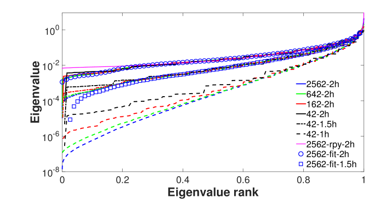
Figure 3: Eigenvalue spectrum of the mobility matrix for steady Stokes flow around a spherical shell covered with different numbers of markers (42, 162, 642, or 2562, see legend) embedded in a periodic domain. Solid lines are for marker spacing of $s\approx 2h$, dashed-dotted lines for spacing $s\approx 1.5\,h$, and dashed lines for spacing of $s\approx 1h$. The marker spacing is $s\approx 1$ in all cases; for $s\approx 2h$, the fluid grid size is $128^{3}$ for 2562 markers and $64^{3}$ for smaller number of markers, and scaled accordingly for other spacings. For comparison, we show the spectrum of $\widetilde{\boldsymbol{\mathcal{M}}}_{RPY}$ for the most resolved model ($N=2562$ markers) at $s/h\approx 2$. Also shown is the spectrum of the empirical (fit) approximation to the mobility $\widetilde{\boldsymbol{\mathcal{M}}}$ for the two larger spacings; for $s\approx h$ our empirical approximation is very poor and includes many spurious negative eigenvalues (not shown).

Figure 3 clearly shows that the number of very small eigenvalues increases as we bring the markers closer to each other, as expected. The increase in the conditioning number is quite rapid, and the condition number becomes $O(10^{6}-10^{7})$ for marker spacings of about one per fluid grid cell. For the conventional choice $s\approx h/2$, the mobility matrix is so poorly conditioned that we cannot solve the constrained Stokes problem in double-precision floating point arithmetic. Of course, if the markers are too far apart then fluid will leak through the wall of the structure. We have performed a number of heuristic studies of leak through flat and curved rigid walls and concluded that $s/h\approx 2$ yields both small leak and a good conditioning of the mobillity, at least for the six-point kernel used here New6ptKernel . Therefore, unless indicated otherwise, in the remainder of this work, we keep the markers about two grid cells apart in both two and three dimensions. It is important to emphasize that this is just a heuristic recommendation and not a precise estimate. We remark that Taira and Colonius, who solve a different Schur complement “modified Poisson equation”, recommend $s/h\approx 1$ to “achieve a reasonable condition number and to prevent penetration of streamlines caused by a lack of Lagrangian points.”

It is important to observe that putting the markers further than the traditional wisdom will increase the “leak” between the markers. For rigid structures, the exact positioning of the markers can be controlled since they do not move relative to one another as they do for an elastic bodies; this freedom can be used to reduce penetration of the flow into the body by a careful construction of the marker grid. In the Conclusions, we discuss alternatives to the traditional marker-based IB method IBFE that can be used to control the conditioning number of the Schur complement and allow for more tightly-spaced markers.

It is worthwhile to examine the underlying cause of the ill-conditioning as the markers are brought close together. One source of ill-conditioning comes from the discrete (finite-dimensional) nature of the fluid solver, which necessarily limits the rank of the mobility matrix. But another contributor to the worsening of the conditioning is the regularization of the delta function. Observe that for a true delta function ($a\rightarrow 0$) in Stokes flow, the pairwise mobility is the length-scale-free Oseen tensor $\sim r^{-1}$, and the shape of the spectrum of the mobility matrix has to be independent of the spacing among the markers. In the standard immersed boundary method, $a\sim h$, so the fluid grid scale $h$ and the regularization scale $a$ are difficult to distinguish.

To try to separate $h$ from $a$, we can take a continuum model of the fluid, but keep the discrete marker representation of the body; see (1). In this case the pairwise mobility would be given by (13), which leads to the RPY tensor (16) for a kernel that is a surface delta function over a sphere of radius $a$ (see (4.1) in RPY_Shear_Wall ). In Fig. 3 we compare the spectra of the discrete mobility $\boldsymbol{\mathcal{M}}$ with those of the analytical mobility approximation $\widetilde{\boldsymbol{\mathcal{M}}}_{RPY}$ constructed by using (16) for the pairwise mobility. We observe that the two are very similar for $s\approx 2h$, however, for smaller spacings $\widetilde{\boldsymbol{\mathcal{M}}}_{RPY}$ does not have very small eigenvalues and is much better conditioned than $\boldsymbol{\mathcal{M}}$ (data not shown). In Fig. 3 we also show the spectrum of our approximate mobility $\widetilde{\boldsymbol{\mathcal{M}}}$ constructed using the empirical fits described in Section IV. The resulting spectra show a worsening conditioning for spacing $s\approx 1.5h$ consistent with the spectrum of $\boldsymbol{\mathcal{M}}$. These observations suggest that both the regularization of the kernel and the discretization artifacts contribute to the ill-conditioning, and suggest that it is worthwhile to explore alternative discrete delta function kernels in the context of rigid-body IB methods.

We also note that we see a severe worsening of the conditioning of $\boldsymbol{\mathcal{M}}$, independent of $\beta$, when we switch from a spherical shell to a filled sphere model. Some of this may be due to the fact that the tetrahedral volume mesh used to construct the marker mesh is not as uniform as the surface triangular mesh. We suspect, however, that this ill-conditioning is primarily physical rather than numerical, and comes from the fact that the present marker model cannot properly distinguish between surface tractions and body (volume) stresses. Therefore, $\boldsymbol{\Lambda}$ remains physically ill-defined even if one gets rid of all discretization artifacts.

Lastly, it is important to emphasize that in the presence of ill-conditioning, what matters in practice are not only the smallest eigenvalues but also their associated eigenvectors. Specifically, we expect to see signatures of these eigenvectors (modes) in $\boldsymbol{\Lambda}$, since they will appear with large coefficients in the solution of (9) if the right hand side has a nonzero projection onto the corresponding mode. As expected, the small-eigenvalue eigenvectors of the mobility correspond to high-frequency (in the spatial sense) modes for the forces $\boldsymbol{\Lambda}$. Therefore, if the markers are too closely spaced the solutions for the forces $\boldsymbol{\Lambda}$ will develop unphysical high-frequency oscillations or jitter, even for smooth flows, especially in time-dependent flows, as observed in practice SmoothingDelta_IBM . We have observed that for smooth flows (i.e., smooth right hand-side of (9)), the improved translational invariance of the 6-point kernel reduces the magnitude of this jitter compared to the traditional Peskin four-point kernel.

VII Numerical Tests

In this section we apply our rigid-body IB method to a number of benchmark problems. We first present tests of the preconditioned FGMRES solver, and then demonstrate the advantage of our method over splitting-based direct forcing methods. We further consider a simple test problem at zero Reynolds number, involving the flow around a fixed sphere, and study the accuracy of both the fluid (Eulerian) variables $\boldsymbol{v}$ and $\pi$, as well as of the body (Lagrangian) surface tractions represented by $\boldsymbol{\Lambda}$, as a function of the grid resolution. We finally study flows around arrays of cylinders in two dimensions and spheres in three dimensions over a range of Reynolds numbers, and compare our results to those obtained by Ladd using the Lattice-Boltzmann method VACF_Ladd ; FiniteRe_2D_Ladd ; SmallRe_3D_Ladd .

VII.1 Empirical convergence of GMRES

Here we consider the model problem of flow past a sphere in a cubic domain that is either periodic or with no-slip boundaries. Except for the largest resolutions studied here, the number of markers is relatively small, and dense linear algebra can be used to solve the mobility subproblem (21) robustly and efficiently, so that the cost of the solver is dominated by the fluid solver. We therefore use the number of total applications of the Stokes preconditioner (22) as a proxy for the CPU effort, instead of relying on elapsed time, which is both hardware and software dependent. A key parameter in our preconditioner is the number of iterations $N_{s}$ used in the iterative unconstrained Stokes solver. We recall that in the full preconditioner, there are two unconstrained inexact Stokes solves per iteration, giving a total of $2N_{s}$ applications of $\boldsymbol{\mathcal{P}}_{S}^{-1}$ per outer FGMRES iteration. If the lower triangular preconditioner is used, then the second inexact Stokes solve is omitted, and we perform only $N_{s}$ applications of $\boldsymbol{\mathcal{P}}_{S}^{-1}$ per outer FGMRES iteration.

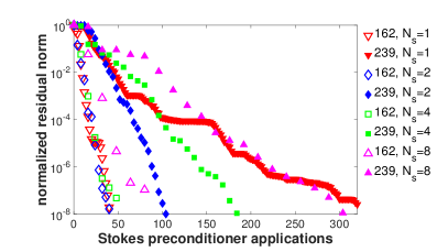
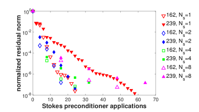
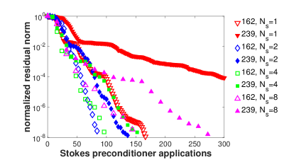
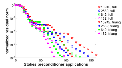
Figure 4: FGMRES convergence for the constrained problem (3) for different numbers of iterations $N_{s}$ in the unconstrained Stokes solver used in the preconditioner. The specific problem is a rigid sphere of hydrodynamic radius $R$ moving through a stationary domain of length $L\approx 4.35\,R$, with the marker spacing fixed at $s/h\approx 2$ and the GMRES restart frequency set to 100 iterations. (Top left panel) Steady Stokes ($Re=0$) flow for an empty 162-marker shell and a filled 239-marker sphere moving through a periodic domain of $32^{3}$ fluid grid cells. (Top right panel) Same as top left but for $Re\approx 10$. (Bottom left panel) As top left panel but now in domain with no slip boundary conditions applied on all sides of the domain. (Bottom right panel) A spherical shell moving in a non-periodic domain (as in bottom left panel) for different resolutions of the shell (162, 642, 2562, and 10242 markers, respectively) and the fluid solver grid ($32^{3}$, $64^{3}$, $128^{3}$, and $256^{3}$ grid cells, respectively), fixing $N_{s}=4$, for both the full Schur complement preconditioner and the lower triangular approximate Schur complement preconditioner.

In the first set of experiments, we use the full preconditioner and periodic boundary conditions. We represent the sphere by a spherical shell of markers that is either empty (162 markers) or is filled with additional markers in the interior (239 markers). The top panels of Fig. 4 show the relative FGMRES residual as a function of the total number of applications of $\boldsymbol{\mathcal{P}}_{S}^{-1}$ for several different choices of $N_{s}$, for both steady Stokes flow (left panel) and a flow at Reynolds number $\text{Re}=10$ (right panel). We see that for spherical shells with well-conditioned $\boldsymbol{\mathcal{M}}$ and $\widetilde{\boldsymbol{\mathcal{M}}}$, the exact value of $N_{s}$ does not have a large effect on solver performance. However, making $N_{s}$ very large leads to wasted computational effort by “over-solving” the Stokes system. This degrades the overall performance, especially for tight solver tolerance. For the ill-conditioned case of a filled sphere model in steady Stokes flow, the exact value of $N_{s}$ strongly affects the performance, and the optimal value is empirically determined to be $N_{s}=2$. As expected, the linear system (3) is substantially easier to solve at higher Reynolds numbers, especially for the filled-sphere models.

In the bottom left panel of Fig. 4 we show the FGMRES convergence for a non-periodic system. In this case, we know that the Stokes preconditioner $\boldsymbol{\mathcal{P}}_{S}^{-1}$ itself does not perform as well as in the periodic case NonProjection_Griffith ; StokesKrylov , and we expect slower overall convergence. In this case, we see that $N_{s}=2$ and $N_{s}=4$ are good choices. Investigations (data not shown) show that $N_{s}=4$ is more robust for problems with a larger number of markers. Also, note that increasing $N_{s}$ decreases the total number of FGMRES iterations for a fixed number of applications of $\boldsymbol{\mathcal{P}}_{S}^{-1}$, and therefore reduces the overall memory usage and the number of times the mobility subproblem (21) needs to be solved; however, note that each of these solves is just a backward/forward substitution if a direct factorization of $\widetilde{\boldsymbol{\mathcal{M}}}$ has been precomputed.

The bottom right panel of Fig. 4 shows the FGMRES convergence for a non-periodic system as the resolution of the grid and the spherical shell is refined in unison, keeping $N_{s}=4$. The results in Fig. 4 demonstrate that our linear solver is able to cope with the increased number of degrees of freedom under refinement relatively robustly, although a slow increase of the total number of FGMRES iterations is observed. Comparing the full preconditioner with the lower triangular preconditioner, we see that the latter is computationally more efficient overall; this is in agreement with experience for the unconstrained Stokes system StokesKrylov . In some sense, what this shows is that it is best to let the FGMRES solver correct the initial unconstrained solution for the velocity and pressure in the next FGMRES iteration, rather than to re-solve the fluid problem in the preconditioner itself. However, if very tight solver tolerance is required, we find that it is necessary to perform some corrections of the velocity and pressure inside the preconditioner. In principle, the second unconstrained Stokes solve in the preconditioner can use a different number of iterations $N_{s}^{\prime}$ from the first, but we do not explore this option further here. Also note that if $\widetilde{\boldsymbol{\mathcal{M}}}\approx\boldsymbol{\mathcal{M}}$ (for example, if it was computed numerically rather than approximated), then the full Schur complement preconditioner will converge in one or two iterations and there is no advantage to using the lower triangular preconditioner.

VII.2 Flow through a nozzle

In this section we demonstrate the strengths of our method on a test problem involving steady-state flow through a nozzle in two dimensions. We compare the steady state flow through the nozzle obtained using our rigid-body IB method to the flow obtained by using a splitting-based direct forcing approach DirectForcing_Uhlmann ; RigidIBAMR . Specifically, we contrast our monolithic fluid-solid solver to a split solver based on performing the following operations at time step $n$:Solve the fluid sub-problem as if the body were not present,

$$\left[\begin{array}[]{cc}\boldsymbol{\mathcal{A}}&\boldsymbol{\mathcal{G}}\\ -\boldsymbol{\mathcal{D}}&\boldsymbol{0}\end{array}\right]\left[\begin{array}[]{c}\tilde{\boldsymbol{v}}^{n+1}\\ \tilde{\pi}^{n+\frac{1}{2}}\end{array}\right]=\left[\begin{array}[]{c}\boldsymbol{g}^{n+\frac{1}{2}}\\ \boldsymbol{0}\end{array}\right].$$

1. Calculate the slip velocity on the set of markers, $\Delta\boldsymbol{V}=-\left(\boldsymbol{\mathcal{J}}^{n+\frac{1}{2}}\tilde{\boldsymbol{v}}^{n+1}+\boldsymbol{W}^{n+\frac{1}{2}}\right)$, giving the fluid-solid force estimate $\boldsymbol{\Lambda}^{n+\frac{1}{2}}=\left(\rho/\Delta t\right)\Delta\boldsymbol{V}$.

2. Correct the fluid velocity to approximately enforce the no-slip condition,

   $$\boldsymbol{v}^{n+1}=\tilde{\boldsymbol{v}}^{n+1}+S^{n+\frac{1}{2}}\Delta\boldsymbol{V}.$$

Note that in the original method of RigidIBAMR in the last step the fluid velocity is projected onto the space of divergence-free vector fields by re-solving the fluid problem with the approximation $\boldsymbol{\mathcal{A}}\approx\left(\rho/\Delta t\right)\boldsymbol{I}$ (i.e., ignoring viscosity). We simplify this step here because we have found the projection to make a small difference in practice for steady state flows, since the same projection is carried out in the subsequent time step.

Figure 5: Two-dimensional flow through a nozzle (top panel) in a slit channel computed by our rigid IB method (left panels) and a simplified version of the splitting-based method of Bhalla et al. RigidIBAMR (right panels). (Top panel) The geometry of the channel along with the (approximately) steady state flow at $\text{Re}\mbox{$\approx$}19$, as obtained using our method. The color plot shows the pressure and the velocity is shown as a vector field. (Middle panels) Flow at $\text{Re}\approx 19$, computed at time $T=10^{2}$. For our method (left) we use a time step size of $\Delta t=5\cdot 10^{-2}$ (corresponding to advective CFL number of $U_{max}\Delta t/\Delta x\approx 0.13$), while for the splitting method (right) we use $\Delta t=10^{-3}$. The streamlines are traced from the entrance to the channel for a time of $T_{s}=7\cdot 10^{3}$ and shown as black lines. (Bottom panels) Same as the middle row but now for $\text{Re}\approx 0.2$, final time $T=10$ and streamlines followed up to $T_{s}=4\cdot 10^{4}$, with $\Delta t=0.125$ for our method (left), and $\Delta t=10^{-3}$ for the splitting method (right).

We discretize a nozzle constriction in a slit channel using IB marker points about 2 grid spacings apart. The geometry of the problem is illustrated in the top panel of Fig. 5; parameters are $\rho=1$, grid spacing $\Delta x=0.5$, nozzle length $l=55.5$, nozzle opening width $d\approx 2.9$, and $\eta$ variable (other parameters are given in the figure caption). No slip boundary conditions are specified on the top and bottom channel walls, and on the side walls the tangential velocity is set to zero and the normal stress is specified to give a desired pressure jump across the channel of $\Delta\pi=2$. The domain is discretized using a grid of $256\times 128$ cells and the problem evolved for some time until the flow becomes essentially steady. The Reynolds number is estimated based on the maximum velocity through the nozzle opening and the width of the opening.

In the bottom four panels in Fig. 5 we compare the flow computed using our method (left panels) to that obtained using the splitting-based direct forcing algorithm summarized above (right panels). Our method is considerably slower (by at least an order of magnitude) for this specific example because the GMRES convergence is slow for this challenging choice of boundary conditions at small Reynolds numbers in two dimensional (recall that steady Stokes flow in two dimensions has a diverging Green’s function). To make the comparison fairer, we use a considerably smaller time step size for the splitting method, so that we approximately matched the total execution time between the two methods. Note that for steady-state problems like this one with fixed boundaries, it is much more efficient to precompute the actual mobility matrix (Schur complement) once at the beginning, instead of approximating it with our empirical fits. However, for a more fair and general comparison we instead use our preconditioner to solve the constrained fluid problem in each time step anew to a tight GMRES tolerance of $10^{-9}$. For this test we use $N_{s}=2$ iterations in the fluid solves inside our preconditioner.

The visual results in the right panels of Fig. 5 clearly show that the splitting errors in the enforcement of the no-slip boundary condition lead to a notable “leak” through the boundary, especially at small Reynolds numbers. To quantify the amount of leak we compute the ratio of the total flow through the opening of the nozzle to the total inflow; if there is no leak this ratio should be unity. Indeed, this ratio is larger than $0.99$ for our method at all Reynolds numbers, as seen in the lack of penetration of the flow inside the body in the left panels in Fig. 5. For $\text{Re}\approx 19$, we find that even after reducing the time step by a factor of 50, the splitting method gives a ratio of $0.935$ (i.e., 6.5% leak), which can be seen as a mild penetration of the flow into the body in the middle right panel in Fig. 5. For $\text{Re}\approx 0.2$, we find that we need to reduce $\Delta t$ by a factor of 1250 to get a flow ratio of $0.94$ for the splitting method; for a time step reduced by a factor of 125 there is a strong penetration of the flow through the nozzle, as seen in the bottom right panel of Fig. 5.

VII.3 Stokes flow between two concentric shells

Steady Stokes flow around a fixed sphere of radius $R_{1}$ in an unbounded domain (with fluid at rest at infinity) is one of the fundamental problems in fluid mechanics, and analytical solutions are well known. Our numerical method uses a regular grid for the fluid solver, however, and thus requires a finite truncation of the domain. Inspired by the work of Balboa-Usabiaga et al. DirectForcing_Balboa , we enclose the sphere inside a rigid spherical shell of radius $R_{2}=4R_{1}$. This naturally provides a truncation of the domain because the flow exterior to the outer shell does not affect the flow inside the shell. Analytical solutions remain simple to compute and are given in Appendix C.

Figure 6: Marker configuration for computing Stokes flow between two concentric spherical shells. Markers are shown as spheres with size on the order of their effective hydrodynamic radius. The inner shell of markers is shown in red, and the outer shell of markers is shown in gray. (Left) Intermediate resolution, inner shell of 162 markers and outside shell of 2562 markers. (Right) Highest resolution studied here, inner shell of 642 markers and outside shell of 10242 markers.

We discretize the inner sphere using a spherical shell of markers, since for steady Stokes flow imposing a rigid body motion on the surface of the inner sphere guarantees a stress-free rigid body motion for the fluid filling the inner sphere RegularizedStokeslets . We use the same recursive triangulation of the sphere, described in Section V, to construct the marker grid for both the inner and outer shells. The ratio of the number of markers on the outer and inner spheres is approximately $16$ (i.e., there are two levels of recursive refinement between the inner and outer shells), consistent with keeping the marker spacing similar for the two shells and a fixed ratio $R_{2}/R_{1}=4$. The fluid grid size is set to keep the markers about two grid cells apart, $s\approx 2h$. The rigid-body velocity is set to $\boldsymbol{V}=\left(1,0,0\right)$ for all markers on the outer shell, and to $\boldsymbol{V}=0$ on all markers on the inner shell. The outer sphere is placed in a cubic box of length $l=4.15R_{2}$ with specified velocity $\boldsymbol{v}=\left(1,0,0\right)$ on all of the boundaries; this choice ensures that the flow outside of the outer shell is nearly uniform and equal to $\boldsymbol{v}=\left(1,0,0\right)$. In the continuum setting, this exterior flow does not affect the flow of interest (which is the flow in-between the two shells), but this is not the case for the IB discretization since the regularized delta function extends a few grid cells on both sides of the spherical shell.

A spherical shell of geometric radius $R_{g}$ covered by markers acts hydrodynamically as a rigid sphere of effective hydrodynamic radius $R_{h}\approx R_{g}+a$ MultiblobSprings , where $a$ is the hydrodynamic radius of a single marker IBM_Sphere ; ISIBM ; BrownianBlobs (we recall that for the six-point kernel used here, $a\approx 1.47\,h$). A similar effect appears in the Lattice-Boltzmann simulations of Ladd, with $a$ being related to the lattice spacing VACF_Ladd ; MultiblobSprings ; FiniteRe_3D_Ladd . When comparing to theoretical expressions, we use the effective hydrodynamic radii of the spherical shells (computed as explained below) and not the geometric radii. Of course, the enhancement of the effective hydrodynamic radius over the geometric one is a numerical discretization artifact, and one could choose not to correct the geometric radius. However, this comparison makes immersed boundary models of steady Stokes flow appear much less accurate than they actually are in practice. For example, one should not treat a line of markers as a zero-thickness object of zero geometric radius; rather, such a line of rigidly-connected markers should be considered to model a rigid cylinder with finite thickness proportional to $a$ IBM_Sphere .

We can measure the effective hydrodynamic radius $R_{h}$ of a spherical shell of markers from the drag force on a periodic cubic lattice of such objects moving with velocity $V$. Specifically, we place a single shell of $N$ markers in a triply-periodic domain with cubic unit cell of length $l$, set $\boldsymbol{V}=\left(1,0,0\right)$ on all markers, solve (3), and measure the total drag force as $F=\sum_{i=1}^{N}\boldsymbol{\Lambda}_{i}$. The periodic correction to the Stokes drag formula is well-known Mobility2D_Hasimoto ,

$$\frac{F}{\eta V}=\frac{6\pi R_{h}}{1-2.8373(R_{h}/l)+4.19(R_{h}/l)^{3}-27.4(R_{h}/l)^{6}+\text{h.o.t.}},$$ (23)

and allows us to obtain a very accurate estimate of $R_{h}$ from the drag for $l\gg R_{h}$. The results are given in the left half of table 1 in the form of the dimensionless ratio $R_{h}/R_{g}$; we see that as the resolution is increased $R_{h}\rightarrow R_{g}$ with an approximately linear rate of convergence, as expected. Since this computation refers to flow outside of the shell of markers, we can call the computed $R_{h}$ the effective outer hydrodynamic radius and use it to set the value of $R_{1}$ in the theory. We use a similar procedure to measure an effective inner hydrodynamic radius $R_{2}$ for the outer spherical shell. Specifically, we obtain $R_{2}$ from the drag on the inner sphere based on the theoretical formula (43), where we use the previously-determined value of $R_{1}$ for the effective radius of the inner sphere. The results are given in the right half of Table 1 and again show that as the grid is refined the hydrodynamic radii converge to the geometric ones.

Table 1: Ratio of the effective hydrodynamic and geometric radii of the inner (left half) and outer (right half) spherical shells for simulations of steady Stokes flow around a fixed sphere embedded within a moving spherical cavity, at different resolutions.

Resolution	Number markers	$R_{h}/R_{g}$		Number markers	$R_{h}/R_{g}$
grid size	Inner shell			Outer shell
$30^{3}$	12	1.48		162	0.93
$60^{3}$	42	1.22		642	0.96
$120^{3}$	162	1.09		2562	0.98
$240^{3}$	642	1.04		10242	0.99

VII.3.1 Convergence of fluid flow (pressure and velocity)

The top panel of Fig. 7 shows a slice through the middle of the nested spherical shells along with the fluid velocity $\boldsymbol{v}$. Recall that the flow inside the inner sphere should vanish, implying that the pressure inside the inner shell should be constant (set to zero here), and the flow outside of the outer sphere should be uniform. The bottom right panel of the figure zooms in around the inner sphere to reveal that there is some spurious pressure gradient and an associated counter-rotating vortex flow generated inside the inner sphere. The bottom right panel shows the error in the computed fluid flow $(\boldsymbol{v},\pi)$, that is, the difference between the computed flow and the theoretical solution given in Appendix C. It is clear that the majority of the error is localized in the vicinity of the inner shell and in the interior of the inner sphere. Note that these errors would be much larger if the theory had used the geometric radii instead of the hydrodynamic radii for the shells.

Figure 7: Flow field around a fixed sphere inside a moving spherical cavity. The outer shell is discretized using 2562 markers, while the inner one has 162 markers, shown as black circles. (Top) Velocity field. (Bottom Left) Zoom of the velocity (vector field) and pressure (color plot) around the inner shell. (Bottom Right) Same as bottom left but now showing the error in the velocity and pressure compared to the theoretical expressions.

Tables 2 and 3 show the norms of the error in the computed flow field as a function of resolution. Asymptotically first-order convergence is observed in the $L_{1}$ and $L_{2}$ norms for both the velocity and the pressure. In the $L_{\infty}$ norm, we expect the velocity to also converge linearly, but we do not expect to see convergence in the pressure, since the velocity is continuous across the interface but the pressure has a jump; this is consistent with the numerical data.

Table 2: Normalized norms of the error in the computed velocity ($\Delta\boldsymbol{v}$) for steady Stokes flow around a fixed sphere embedded within a moving spherical cavity, at different resolutions (see two left-most columns). An estimated order of convergence based on successive refinements is indicated in the column to the right of the corresponding error norm.

Markers	Resolution	$||\Delta\boldsymbol{v}||_{1}/||\boldsymbol{v}||_{1}$	Rate	$||\Delta\boldsymbol{v}||_{2}/||\boldsymbol{v}||_{2}$	Rate	$||\Delta\boldsymbol{v}||_{\infty}/||\boldsymbol{v}||_{\infty}$	Rate
162-12	$30^{3}$	$4.08\cdot 10^{-2}$		$6.39\cdot 10^{-2}$		0.558
642-42	$60^{3}$	$1.14\cdot 10^{-2}$	1.83	$2.08\cdot 10^{-2}$	1.62	0.322	0.79
2562-162	$120^{3}$	$4.61\cdot 10^{-3}$	1.30	$8.74\cdot 10^{-3}$	1.24	0.160	1.01
10242-642	$240^{3}$	$2.16\cdot 10^{-3}$	1.09	$4.26\cdot 10^{-3}$	1.04	0.091	0.82

Table 3: Normalized norms of the error in the pressure ($\Delta\pi$) for steady Stokes flow around a fixed sphere embedded within a moving spherical cavity, at different resolutions (see two left-most columns). An estimated order of convergence based on successive refinements is indicated in the column to the right of the corresponding error norm.

Markers	Resolution	$||\Delta\pi||_{1}/||\pi||_{1}$	Rate	$||\Delta\pi||_{2}/||\pi||_{2}$	Rate	$||\Delta\pi||_{\infty}/||\pi||_{\infty}$	Rate
162-12	$30^{3}$	$0.849$		0.788		1.0
642-42	$60^{3}$	0.567	0.58	0.486	0.70	1.0	0.0
2562-162	$120^{3}$	$0.344$	0.72	0.275	0.82	0.860	0.22
10242-642	$240^{3}$	$0.196$	0.81	0.164	0.75	0.704	0.29

VII.3.2 Convergence of Lagrangian forces (surface stresses)

The first-order convergence of the pressure and velocity is expected and well-known in the immersed boundary community. The convergence of the tractions $\left(\boldsymbol{\sigma}\cdot\boldsymbol{n}\right)$ on the fluid-body interface is much less well studied, however. This is in part because in penalty-based or splitting methods, it is difficult to estimate tractions precisely (e.g., for penalty methods using stiff springs, the spring tensions oscillate with time), and in part because a large number of other studies have placed the markers too closely to obtain a well-conditioned mobility matrix and thus to obtain accurate forces. Furthermore, there are at least two ways to estimate surface tractions in IB methods, as discussed in extensive detail in Ref. Tractions_Fauci . One method is to estimate fluid stress from the fluid flow and extrapolate toward the boundary. Another method, which we use here, is to use the computed surface forces $\boldsymbol{\Lambda}$ to estimate the tractions.

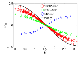
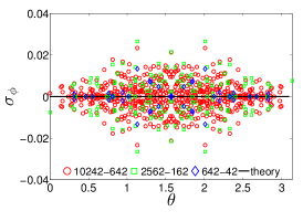
Figure 8: Convergence of surface stresses to their theoretical values for the three different resolutions. Pointwise traction estimates are shown with symbols as a function of the angle $\theta$ relative to the direction of the flow, while the theory is shown with a solid black line. (Left columns) Normal component of the traction $\sigma_{n}=\hat{\boldsymbol{r}}\cdot\boldsymbol{\sigma}\cdot\boldsymbol{n}$. (Center columns) Tangential component of traction in direction of flow, $\sigma_{\theta}=\hat{\boldsymbol{\theta}}\cdot\boldsymbol{\sigma}\cdot\boldsymbol{n}$. (Right columns) Tangential component in the direction perpendicular to the flow, $\sigma_{\phi}=\hat{\boldsymbol{\phi}}\cdot\boldsymbol{\sigma}\cdot\boldsymbol{n}$, which should vanish by symmetry. (Top row) Different resolutions (see legend) for a fixed spacing $s\approx 2h$. Note that for the coarsest resolution of only 12 markers on the inner sphere, the computed tractions have values off the scale of this plot and are thus not shown. (Bottom row) The most resolved case of $2562-162$ markers for different spacing between markers, as indicated in the legend. Note that using $s\approx h$ leads to severe ill-conditioning and the computed tractions show random scatter well beyond the scale of the plot and are thus not shown.

We obtain pointwise estimates of the tractions at the positions of the markers from the relation $\left(\boldsymbol{\sigma}\cdot\boldsymbol{n}\right)\left(\boldsymbol{R}_{i}\right)\approx\boldsymbol{\Lambda}_{i}/\Delta A_{i}$, where $\Delta A_{i}$ is the surface area associated with marker $i$. We obtain $\Delta A_{i}$ from the surface triangulation used to construct the marker of grids by assigning one third of the area of each triangle to each of its nodes. In Fig. 8 we show the computed normal and tangential components of the traction in polar coordinates, with the $z$ symmetry axes along the direction of the flow. The theoretical prediction given in Appendix C is shown with a black line and is based on the geometric radii.

The top row of Fig. 8 shows the computed tractions for several resolutions with marker spacing $s\approx 2h$. It is seen that as the grid is refined, the computed tractions appear to converge pointwise to the correct values. However, the convergence is very slow, and even for the large resolutions reported here, it is evident that the asymptotic convergence regime has not been reached. Consequently, no precise statement about the order of convergence can be made from these data. At lower resolution, some of the results even show qualitatively wrong behavior. For example, the normal traction $\sigma_{n}=\boldsymbol{n}\cdot\boldsymbol{\sigma}\cdot\boldsymbol{n}$ for a resolution of 42 inner and 642 outer markers grows with $\theta$, but the theoretical result decreases with $\theta$. We also see scatter in the values among individual markers, indicating that the geometrical and topological non-uniformity of the marker grid affect the pointwise values.

Nonetheless, we remark that low-order moments of the surface tractions are much more accurate than the pointwise tractions. For example, the total drag on the inner sphere is much more accurate, as seen in Table 1. Other test problems not reported here indicate that stresslets are also computed quite accurately, especially if one accounts for the distinction between geometric and hydrodynamic radii. These findings suggest that weak convergence of the tractions is more robust than strong convergence. In fact, lower order moments can show reasonable behavior even if the marker spacing is small and the pointwise forces are numerically unstable to compute. Somewhat unsurprisingly, we find that the pointwise traction estimates are improved as the spacing among the markers is increased; see the bottom row in Fig. 8. The improvement is not only due to the reduction of the scatter, as expected from the improvement in conditioning number of the mobility matrix, but also due to global reduction of the error in the tractions; the observed global reduction may, however, be specific to steady Stokes flow. For widely spaced markers, however, the error in the computed flow field field will increase because the flow will penetrate the shell boundary. This once again demonstrates the delicate balance that is required in choosing the marker spacing for rigid bodies, as we discuss further in the Conclusions.

VII.4 Steady Stokes flow around sphere in a slit channel

In this section we study a problem at zero Reynolds numbers with nontrivial boundary conditions, namely, steady Stokes flow around a sphere in a slit channel (flow between two parallel walls). It is well-known that computing flows in such geometries using Green’s function based methods such as boundary-integral methods is highly-nontrivial BD_LB_Ladd ; BoundaryIntegral_Wall ; StokesianDynamics_Slit . Specific methods for spheres in a channel have been developed HE_Spheres_TwoWalls but these are not general, in particular, flow in a square channel requires a different method, and incorporating the periodicity in some of the dimensions is nontrivial BoundaryIntegral_Periodic3D ; BoundaryIntegral_Wall . At the same time, we wish to point out that boundary-integral methods have some advantages over our IB method as well. Notably, they are considerably more accurate, and handling domains unbounded in one or more directions is possible by using the appropriately-decaying Green’s function.

Unlike the case of a single no-slip boundary, writing down an analytical solution for slit channels is complex and requires numerically-evaluating the coefficients in certain series expansions StokesianDynamics_Slit . For the component of the mobility $\mu=F/V$ of a sphere in an infinite slit channel, Faxen has obtained exact series expansions for the mobility at the half and quarter channel locations,

$$\mu_{\parallel}\left(H=\frac{d}{2}\right) = \frac{1}{6\pi\eta R_{h}}\Bigg{[}1-1.004\frac{R_{h}}{H}+0.418\frac{R_{h}^{3}}{H^{3}}+0.21\frac{R_{h}^{4}}{H^{4}}-0.169\frac{R_{h}^{5}}{H^{5}}+\dots\Biggr{]}$$

$$\mu_{\parallel}\left(H=\frac{d}{4}\right) = \frac{1}{6\pi\eta R_{h}}\Biggl{[}1-0.6526\frac{R_{h}}{H}+0.1475\frac{R_{h}^{3}}{H^{3}}-0.131\frac{R_{h}^{4}}{H^{4}}-0.0644\frac{R_{h}^{5}}{H^{5}}+\dots\Biggr{]}$$ (24)

where $R_{h}$ is the (hydrodynamic) radius of the sphere, $H$ is the distance from the center of the particle to the nearest wall, and $d$ is the distance between the walls.

To simulate a spherical particle in a slit channel we place a single spherical shell with different number of IB markers in a domain of size $L\times L\times d$, at either a quarter or half distance from the channel wall. No slip walls are placed at $z=0$ and $z=L$, and periodic boundary conditions are applied in the $x$ and $y$ directions. For each $L$, we compute an effective hydrodynamic radius $R_{L}$ by assuming (24) holds with $R_{h}$ replaced by $R_{L}$. We know that as $L\rightarrow\infty$ we have $R_{L}\rightarrow R_{h}$, however, we are not aware of theoretical results for the dependence $R_{L}(L)$ at finite $L$. In Fig. 9, we plot $R_{L}/R_{h}-1$ versus $R_{h}/L$ for $d\approx 8R_{h}$. Here the effective hydrodynamic radius of the shell $R_{h}$ is estimated by using (23), as shown in Table 1 (see inner radius). We see that we have consistent data for $R_{L}(L)$ among different resolutions, and we obtain consistency in the limit $L\rightarrow\infty$. This indicates that even a low-resolution model with as few as 12 markers offers a reasonably-accurate model of a sphere of effective radius $R_{h}$, independent of the boundary conditions.

Figure 9: Effective hydrodynamic radius $R_{L}(L)$ of a sphere of hydrodynamic radius $R_{h}$, translating parallel to the walls of a slit channel of dimensions $L\times L\times d$. Red symbols are for the sphere at the midplane of the channel, $H/d=0.5$, and blue symbols are for $H/d=0.25$; these two give different dependence $R_{L}(L)$ as expected. The channel width is taken $d\approx 8R_{H}$ and different numbers of markers are used for the sphere (see legend), and the grid spacing is set to give a marker spacing $s$ as close as possible to $a/s\approx 0.5$. Note that similar to the example of flow between concentric spheres the correct value of the drag is determined by the larger hydrodynamic and not by the geometric radius of the shell.

VII.5 Steady Stokes flow around cylinders

Here we study the drag force on a periodic square array of cylinders (i.e., disks in two dimensions) with lattice spacing $l$. The corresponding study in three dimensions is presented in Section VII.7. The equivalent of (23) in two dimensions for dilute systems is Mobility2D_Hasimoto ; FiniteRe_2D_Ladd

$$\frac{F}{\eta V}=\frac{4\pi}{-\ln(\sqrt{\phi})-0.738+\phi-0.887\phi^{2}+2.038\phi^{3}+O\left(\phi^{4}\right)},$$ (25)

where $\phi=\pi R_{h}^{2}/l^{2}$ is the packing fraction of the disks and $R_{h}$ is the hydrodynamic radius of the cylinder, which is defined from (25). Observe that in two dimensions, there is no limit as $\phi\rightarrow 0$, in agreement with Stokes’s paradox for flow around a single cylinder; one must account for inertial effects for very small volume fractions in order to obtain physically-relevant results. Table 4 reports $R_{h}$ for several different marker models of a cylinder, as estimated by computing the drag for a range of packing fractions and extrapolating to $\phi\ll 1$ using (25). As expected, the more resolved the cylinder, the closer $R_{h}$ is to $R_{g}$. Filling the cylinder with markers both substantially enlarges the effective hydrodynamic radius and also degrades the conditioning of the mobility matrix, and is therefore not advised at zero Reynolds number.

Table 4: Hydrodynamic radii of several discretizations of a cylinder with different numbers of markers on the surface and the interior of the body, keeping $s/h\approx 2$. Two models have markers only on the surface of the cylinder (see the right panel of Fig. 12 for a 39-marker shell). The rest of the models are constructed from a regular polar grid of markers filling the interior of the cylinder (see, for example, left panel of Fig. 12 for a 121-marker cylinder).

Number markers	Surface markers	Interior markers	$R_{h}/R_{g}$
39 shell	39	0	1.04
121 cylinder	37	84	1.15
100 shell	100	0	1.02
834 cylinder	100	734	1.03

Another interesting limit for which there are theoretical results is the dense limit, in which the disks/cylinders almost touch, so that there is a lubrication flow between them. In this limit FiniteRe_2D_Ladd ,

$$\frac{F}{\eta V}\approx\frac{9\pi}{2^{\frac{3}{2}}}\varepsilon^{-\frac{5}{2}},$$ (26)

where $\varepsilon=1-\sqrt{4\phi/\pi}=\left(l-2R_{h}\right)/l$ is the relative gap between the particles. Note that because the number of hydrodynamic cells must be an integer, we cannot get an arbitrary gap between the cylinders for a given cylinder model and fixed $s/h$ (i.e., a fixed $R_{h}/R_{g}$). Also note that when the gap between the cylinders is too small, the kernels from markers on two cylinders start to overlap, and the problem becomes ill-conditioned; we have been able to compute reliable results down to a relative gap of $\varepsilon\gtrsim 10^{-2}$ for the resolutions studied here.

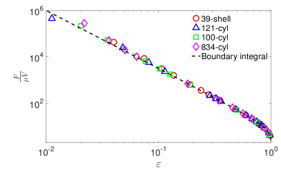
Figure 10: The drag coefficient for a periodic array of cylinders in steady Stokes flow for different resolutions (see Table 4). (Left) As function of volume fraction, compared to the results of a highly-accurate boundary-integral method. (Right) Zoom in for close-packed arrays with inter-particle gap plotted on a log scale to show the asymptotic $\varepsilon^{-\frac{5}{2}}$ divergence of the lubrication force.

Numerical results for the normalized drag over a broad range of volume fractions are shown in Fig. 10 and compared to results obtained using an in-house two-dimensional version of the spectrally-accurate boundary integral method proposed in Ref. BoundaryIntegral_Periodic3D . We obtain very good agreement, similar to that observed using the Lattice Boltzmann method FiniteRe_2D_Ladd , indicating that even moderately-resolved cylinders are good representations so long as one uses their hydrodynamic rather than their geometric radius when computing the effective volume fraction. In particular, in the right panel, we obtain excellent agreement with the lubrication result (26), seeing an increase in the drag of over six orders of magnitude consistent with theory. Of course, the IB method results for the drag do not have a true divergence as $\epsilon\rightarrow 0$ because of the regularization of the singular kernel; one must use adaptively-refined non-regularized boundary integral methods to truly resolve the divergence. In practice, however, effects not included in the theoretical model, such as surface roughness or partial slip, will mollify the unphysical divergence.

VII.6 Unsteady flow around cylinders

Next, we examine the ability of our rigid-body IB method to model unsteady two-dimensional flow around cylinders (disks). We define Reynolds number by

$$\text{Re}=\frac{\rho VR_{h}}{\eta}=\frac{VR_{h}}{\nu},$$

where $R_{h}$ is the hydrodynamic radius of the cylinder measured at $\text{Re}=0$ (see table 4), and $V$ is the velocity of the incident flow. For small Reynolds numbers, the mean drag per unit length $F$ is given by FiniteRe_2D_Ladd

$$\frac{F}{\eta V}=k_{0}+k_{2}\text{Re}^{2},$$

where $k_{0}\left(\phi\right)$ and $k_{2}\left(\phi\right)$ are constants that depend on the packing fraction $\phi$ (defined using the hydrodynamic radius). In the range $\text{Re}\sim 2-5$, the drag becomes quadratic in the flow rate FiniteRe_2D_Ladd , and for moderate Reynolds numbers, a drag coefficient is defined from the empirical relation

$$C_{D}=\frac{F}{\rho V^{2}R_{h}}.$$

As the Reynolds number is increased, the flow becomes unsteady and vortex shedding occurs, and eventually there is a transition to three-dimensional flow. Here we focus on steady flow at $\text{Re}\leq 100$.

A staggered-grid variant of the piecewise-parabolic Godunov method is used for spatial discretization of the advective terms, as explained in detail by Griffith NonProjection_Griffith . In our tests, the time step size is determined by fixing the advective Courant number $V\Delta t/h=0.1$; this value is well bellow the stability limit and ensures that the discretization errors coming from the (unconstrained) fluid solver are small. The Adams-Bashforth method is used to handle advection explicitly. The viscous terms are handled implicitly using the backward Euler method rather than the implicit midpoint rule because we are interested in steady states and not transient phenomena. We initialize the simulations with the fluid moving at a uniform velocity but allow enough time for a steady-state to be reached.

VII.6.1 Drag on periodic array of disks

The permeability of a periodic array of aligned cylinders is a well-studied problem and can be computed by placing a single cylinder in a periodic domain. To create flow through the periodic system, we follow Ladd et al. FiniteRe_3D_Ladd ; FiniteRe_2D_Ladd and apply a constant body force $\boldsymbol{f}$ throughout the domain (including in the interior of the body). We solve the constrained time-dependent problem to a steady state, keeping the cylinder at rest, and measure the average velocity in the domain, $\bar{\boldsymbol{v}}=\text{\text{vol}}^{-1}\,\int_{V}\boldsymbol{v}\,d\boldsymbol{r}.$ In two spatial dimensions, the dimensionless drag coefficient is defined by

$$k=\frac{F_{x}}{\eta\bar{v}_{x}},$$

where the force $\boldsymbol{F}=\text{\text{vol}}\,\boldsymbol{f}=-\boldsymbol{1}^{T}\boldsymbol{\Lambda}$ is the total force applied to the fluid, which must also equal the negative of the total force exerted on the rigid body.

Theory suggests that the correction to the drag scales as $\text{Re}^{2}$ for small Reyonds numbers due to the anti-symmetry of the correction to the flow (relative to steady Stokes) of order Re FiniteRe_2D_Ladd , so that

$$k=k_{0}+k_{2}\text{Re}^{2},$$ (27)

where the values $k_{0}(\phi)$ and $k_{2}(\phi)$ depend on the packing fraction $\phi$. To obtain $k_{0}$, we move the body at a constant velocity and obtain the drag force $\boldsymbol{1}^{T}\boldsymbol{\Lambda}$ from the solution of the constrained steady Stokes problem (11). Because marker-based models of rigid bodies do not have perfect symmetry, the force $\boldsymbol{f}_{0}=-\text{\text{vol}}^{-1}\,\left(\boldsymbol{1}^{T}\boldsymbol{\Lambda}\right)$ has small nonzero components in the direction perpendicular to the flow. To ensure that in the limit $\text{Re}\rightarrow 0^{+}$ we have perfect consistency between the finite Re and zero Re computations, we use the force $\boldsymbol{f}=\left(k/k_{0}\right)\boldsymbol{f}_{0}$ to drive the flow at finite Re numbers. Note that it can take thousands of time steps for the steady state to be established for $\text{Re}\gtrsim 1$; to accelerate convergence, we initialize the computation for a given Re from the steady state for the closest smaller Re. Also note that the exact mobility matrix $\boldsymbol{\mathcal{M}}$ and its factorization can be precomputed once at the beginning and used repeatedly for these steady-state calculations.

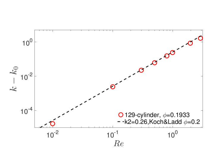
Figure 11: The dimensionless excess (over Stokes flow) drag coefficient for a square array of disks with packing fraction $\phi\approx 0.193$ (129-marker filled cylinder model, fluid grid of $64^{2}$ cells). Comparison is made to known small-Re dependence of the form $k_{0}+k_{2}\text{Re}^{2}$, with the coefficients $k_{0}$ and $k_{2}$ taken from the work of Koch and Ladd FiniteRe_2D_Ladd at $\phi=0.2$.

Fig. 11 shows the dimensionless excess drag $k-k_{0}$ as a function of Re at packing fraction $\phi=0.193$, which is close to the packing fraction $\phi=0.2$ studied using the Lattice-Boltzmann method in Ref. FiniteRe_2D_Ladd . We see very good agreement of the theoretical formula (27) with our results using the values of $k_{0}=49.2$ and $k_{2}=0.24$, which are in good agreement with the values of $k_{0}=51.2$ and $k_{2}=0.26$ given in the caption of Fig. 1 in Ref. FiniteRe_2D_Ladd .

VII.6.2 Flow past a periodic column of cylinders

Here we compute several solutions for flow past a column of cylinders at somewhat larger Reynolds numbers, mimicking the setup of Ladd VACF_Ladd . The domain is a long narrow channel of $2048\times 128$ grid cells with grid spacing $h=0.5$, keeping the markers at a distance $2h$. Periodic boundary conditions are used in the direction of the short side of the channel ($y$). The flow is driven by “uniform” inflow and outflow boundary conditions in the long direction ($x$). Specifically, we impose a specified normal velocity $V$ and zero tangential velocity at both ends of the channel . The center of the cylinder is fixed at a quarter channel length from the inlet. The cylinders in the periodic column are separated by approximately 10 hydrodynamic radii in the $y$ direction (the separation is $9.958R_{h}$ for the 121-marker cylinder, and $9.875R_{h}$ for the 39-marker shell).

Figure 12: Steady incompressible flow at $\text{Re}=10$ past a periodic column of cylinders represented as either filled disks of $121$ markers (left) or a shell of $39$ markers (right). We show the magnitude of the Eulerian constraint force $\boldsymbol{\mathcal{S}}\boldsymbol{\Lambda}$ (gray color map), the streamlines outside of the wake (solid blue lines), the wake velocity field (black arrows), and the Lagrangian constraint forces associated with each marker (color arrows). The red arrow marks the stagnation point where $v_{x}=0$, as used to determine the wake length.

Representative flow fields are shown in Fig. 12 for $\text{Re}=10$ for a filled cylinder model (left) and an empty shell model (right). Note that for the computation of total drag on a fixed cylinder either model can be used since the spurious flow seen inside the empty shell does not generate any overall acceleration of the fluid inside the body. Also note that the spurious counter-rotating vortex pair inside the shell diminishes under refinement, at an approximately linear convergence rate, just as for steady Stokes flow. Computed drag coefficients $k$ and wake lengths are shown in Table 5, and good agreement is seen with the results of Lattice-Boltzmann and finite difference schemes VACF_Ladd . The wake length measures the distance from the cylinder center to the stagnation point, which is obtained by finding the largest $x$ coordinate on the contour of zero horizontal velocity, $v_{x}=0$.

Table 5: Numerical results for steady flow past a periodic column of cylinders at different Reynolds number, for two different models of the body (see Fig. 12), either a filled cylinder or an empty shell of markers. For comparison we reproduce the results in Table 5 in VACF_Ladd , which are computed either using either a Lattice-Boltzmann (LB) or a finite difference (FD) method. (Left) Mean drag coefficient. (Right) Wake length in units of $R_{h}$.

Re	121 cyl	39 shell	LB	FD
5	4.31	4.35	4.21	4.32
10	2.96	2.99	2.91	2.98
20	2.16	2.19	2.17	2.19
50	1.55	1.58	1.67	1.61

Re	121 cyl	39 shell	LB	FD
5	1.52	1.40	1.5	1.49
10	2.55	2.59	2.6	2.65
20	4.50	4.61	4.7	4.74
50	9.96	9.91	10.7	10.3

VII.7 Flow past periodic arrays of spheres

Finally, we study the drag on a cubic arrays of spheres of radius $a$ at zero and finite Reynolds numbers, and compare our results to those of Hill et al. FiniteRe_3D_Ladd . At small packing (volume) fractions $\phi$ and Reynolds numbers, according to Eqs. (1-2) in SmallRe_3D_Ladd , $F-F_{0}=3\text{Re}/8+\mbox{h.o.t.}$ if $\sqrt{\phi}\ll\text{Re}\ll 1$, or, more relevant to our study, $F-F_{0}\sim\text{Re}^{2}/\sqrt{\phi}$ if $\text{Re}\ll\sqrt{\phi}\ll 1$. For small Re and at larger densities, the theoretical arguments in FiniteRe_3D_Ladd ; FiniteRe_2D_Ladd predict that the dimensionless drag is quadratic in Re because the linear term vanishes by symmetry, so that

$$k=\frac{F}{6\pi\eta aV}\approx k_{0}+k_{2}\text{Re}^{2}.$$

For larger Re, the dependence is expected to switch to linear in Re.

Here we focus on close-packed cubic lattices of spheres with packing fraction $\phi=\pi/6\approx 0.5236$. Note that unlike the case of two spatial dimensions, in three dimensions the flow does not need to squeeze in-between the (nearly) touching bodies, so the drag does not diverge even at close packing. The value of the steady Stokes drag $k_{0}$ is tabulated in Table 6 for several resolutions. Different resolutions are examined: an empty shell (see Table 1) of 162 (grid size is $16^{3}$) or 642 markers ($30^{3}$ grid), as well as a filled sphere of 56 (42 on the surface, $10^{3}$ grid) or 239 (162 on the surface, $16^{3}$ grid) markers; the actual value of the packing fraction based on the effective hydrodynamic radius of the model is indicated in the table. A large difference is seen between the filled and empty shell models at this high packing fractions because the spheres are very close to each other and discretization artifacts become pronounced. We have also performed simulations at a lower (but still high) packing fraction of $\phi=0.44$, and there we see much better agreement between the filled and empty sphere models; note that at small $\phi\ll 1$ the value of $k_{0}$ must match among resolutions since we define the packing fraction from $R_{h}$, which is itself determined from the value of $k_{0}$ at small $\phi$ using (25).

Table 6: Dimensionless drag force $k_{0}$ for steady Stokes flow ($Re=0$) past a simple-cubic array of spheres at volume fraction $\phi\approx\pi/6$ (close packing). For the highest-resolution LB simulations in VACF_Ladd the reported value is $k_{0}=42.8$.

Number of markers	$\phi$	$k_{0}$
56 filled	0.5236	40.08
239 filled	0.5238	40.73
162 shell	0.5213	44.49
642 shell	0.5236	43.29

Numerical results for the dimensionless drag coefficient $k$ near the close-packed density $\phi\approx 0.52$ are shown in Fig. 13. Because our discrete models of spheres do not have the same symmetry as a perfect sphere, we numerically observe a small $O(\text{Re})$ correction that can dominate the true correction $k_{2}\text{Re}^{2}$ for $\text{Re}\ll 1$; this is especially evident in the right panel of Fig. 13 for coarsely-resolved models (e.g., a 56-marker sphere) . Empirical fits to literature data for $k_{0}$, $k_{1}$, $k_{2}$, and the range of Re values over which the various fits are valid are tabulated in Ref. EmpiricalDrag_3D . Fig. 13 compares our results to these fits, as well as to reference results obtained using the Lattice Boltzmann method VACF_Ladd at close packing. We observe the expected switch from linear to quadratic dependence on Re and also a reasonable agreement with the literature data, and the agreement appears to improve with increasing resolution.

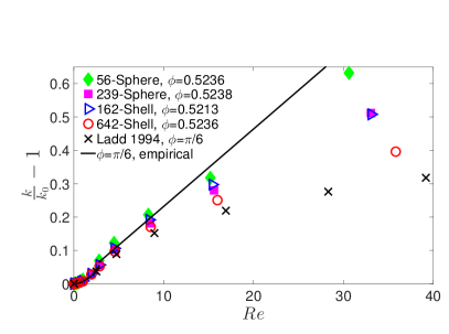
Figure 13: Numerical values (symbols) for the drag coefficient of a periodic array of spheres close packed in a cubic lattice of volume fraction $\phi=\pi/6\approx 0.52$, for several resolutions (see legend), using a linear (left) or log scaling (right). Comparison is made to empirical formulas given in EmpiricalDrag_3D (lines), as well as Lattice Boltzmann results for close-packed cubic arrays given in Table 6 in VACF_Ladd (crosses).

VIII Conclusions

This paper develops an immersed boundary method that enforces strict rigidity of immersed bodies at both zero and finite Reynolds numbers. Unlike existing approaches, we do not rely on penalty or splitting approaches, and we instead directly solve a saddle-point system that couples the fluid velocity and pressure to the unknown rigidity forces. We developed a physics-inspired approximation $\widetilde{\boldsymbol{\mathcal{M}}}$ to the Schur complement (mobility matrix) $\boldsymbol{\mathcal{M}}$ of the constrained system, based on analytical considerations for a continuum fluid model, and demonstrated that this leads to a robust preconditioner so long as the immersed boundary markers are kept sufficiently far to ensure a well-conditioned mobility matrix. Contrary to common practice, we found that the markers should be kept approximately two fluid grid cells apart in rigid-body models in order to obtain accurate and stable pointwise estimates for the traction. We tested our method on a number of standard test problems in both two and three spatial dimensions, and at both zero and finite Reynolds number, and we observed good agreement with theory and literature values. Although in this work we focused on rigid bodies, our method can directly be applied to study fluid flow around bodies with specified kinematics. For example, it can be used to model the flow around a swimming body deforming with a specified gait. We have implemented the method described here in the open-source IBAMR software infrastructure IBAMR in the hope it will be useful to other users of the IB method.

Another challenge that we did not explore here is the efficient computation of the action of $\widetilde{\boldsymbol{\mathcal{M}}}^{-1}$ when there are many markers present; there are many approximate solvers and emerging fast solvers we plan to explore in the future. Of course, using dense linear algebra to solve (21) is likely to be suboptimal, as these solves have $O(N^{2})$ memory complexity and $O(N^{3})$ time complexity. The problem of solving a linear systems similar in structure to (21) appears in many other methods for hydrodynamics of suspensions, including Brownian BrownianDynamics_OrderN ; BrownianDynamics_FMM and Stokesian BrownianDynamics_OrderNlogN dynamics, the method of regularized Stokeslets RegularizedStokeslets_2D ; RegularizedStokeslets , computations based on bead models of rigid bodies HYDROLIB ; SphereConglomerate ; HYDROPRO ; HYDROPRO_Globular , and first-kind boundary integral formulations of Stokes flow BoundaryIntegral_Pozrikidis . Similar matrices appear in static Poisson problems such as electrostatics or reaction-diffusion models ReactiveBlobs , and there is a substantial ongoing work that can be applied to our problem. Notably, the approximate mobility matrix $\widetilde{\boldsymbol{\mathcal{M}}}$ is dense but has a well-understood low-rank structure that can be exploited. Specifically, matrix-vector products $\widetilde{\boldsymbol{\mathcal{M}}}\boldsymbol{\Lambda}$ can be performed in almost linear time using the Fast Multipole Method RPY_FMM . If the condition number of $\widetilde{\boldsymbol{\mathcal{M}}}$ is not too large, one can solve linear systems involving $\widetilde{\boldsymbol{\mathcal{M}}}$ efficiently using an unpreconditioned Krylov solver. For poorly conditioned cases, however, a good preconditioner based on an approximate factorization of $\widetilde{\boldsymbol{\mathcal{M}}}$ is required. In recent years, several approximate low-rank factorizations of matrices of this type have been developed FastHierarchicalSolver ; FastSolver_Ho ; HODLR_BDLR , and can be used as preconditioners in Krylov methods. We have had reasonable success using a fast hierarchically off-diagonal low-rank (HODLR) factorization code developed by Ambikasaran and Darve FastHierarchicalSolver , with significant improvement offered by a recently-developed boundary distance low-rank approximation HODLR_BDLR . Preliminary results indicate great promise for the inverse fast multipole (iFMM) method iFMM ; we have been able to use iFMM to solve the system (21) for as many as $5\cdot 10^{5}$ markers to a relative tolerance of $10^{-8}$. These methods are, however, still under active development, and a significant amount of investigation is necessary to integrate them into the method described here. Notably, we only require an approximate solver for (21) and the impact of the innacuracy in solving (21) on the overall convergence of the outer Krylov solver needs to be assessed.

The type of linear system we solve here is closely connected to those appearing in implicit immersed boundary methods IBM_Implicit_Comparison ; IBMultigrid_Guy ; ImplicitIB_Projection . It is in fact possible to recast the saddle-point problem we consider here into a form closely-related to that appearing in implicit IB methods; the Schur complement for this system is in Eulerian rather than Lagrangian variables as it was for this work, and involves the matrix

$$\boldsymbol{\mathcal{L}}_{v}+\kappa\boldsymbol{\mathcal{S}}\left(\boldsymbol{\mathcal{J}}\boldsymbol{\mathcal{S}}\right)^{-1}\boldsymbol{\mathcal{J}},$$ (28)

for some constant $\kappa$ that does not need to go to infinity. It may be that geometric multigrid methods IBMultigrid_Guy developed for implicit IB methods can be applied to the Eulerian Schur complement (28). At the same time, techniques developed herein may be useful in the development of more efficient implicit IB methods for nearly-rigid bodies.

Our work is only the first step toward the ultimate goal of developing methods able to handle large numbers of rigid bodies in flow. Several computational challenges need to be tackled to realize this goal. Firstly, and most importantly, it is crucial to develop a preconditioner for the enlarged linear system (LABEL:eq:free_kinematics_Stokes) that appears in the context of freely-moving rigid bodies. An additional Schur complement appears when solving this saddle-point problem, and the challenge for future work is approximating the body mobility matrix $\boldsymbol{\mathcal{N}}=\left(\boldsymbol{\mathcal{K}}^{\star}\boldsymbol{\mathcal{M}}^{-1}\boldsymbol{\mathcal{K}}\right)^{-1}.$ Initial investigations have shown great promise in block-diagonal preconditioners with one block per body. In this approach, we neglect the hydrodynamic interactions between bodies, but use the mobility approximation developed in this work together with dense linear algebra for each body.

In the marker-based method described in this work, one must adjust the marker spacing to be “neither too small nor too large”. The sensitivity of the solver performance and the numerical results to the exact spacing of the markers, which comes from the ill-conditioning of the mobility matrix, is one of the key deficiencies of the marker-based representation inherent to the traditional IB method. Recently, Griffith and Luo have proposed an alternative IB approach that models the deformations and stresses of immersed elastic body using a finite element (FE) representation IBFE . In their IB/FE approach, the degrees of freedom associated with $\boldsymbol{\Lambda}$ are represented on an FE mesh that may be coarser than the fluid grid, and the interaction between the fluid grid and body mesh is handled by placing IB markers at the numerical quadrature points of the FE mesh. When such an approach is generalized to rigid bodies, the conditioning of the mobility becomes much less sensitive to the marker spacing. Using a finite-element basis to represent the unknown fluid-body interaction force amounts to applying a filter $\boldsymbol{\Psi}$ to the marker-based mobility matrix, which is a well-known and robust technique to regularize ill-conditioned systems. Specifically, in the context of the IB/FE approach, the mobility operator becomes

$$\boldsymbol{\mathcal{M}}_{FE}=\boldsymbol{\Psi}\left(\boldsymbol{\mathcal{J}}\boldsymbol{\mathcal{L}}^{-1}\boldsymbol{\mathcal{S}}\right)\boldsymbol{\Psi}^{T}=\boldsymbol{\Psi}\boldsymbol{\mathcal{M}}\boldsymbol{\Psi}^{T},$$

where $\boldsymbol{\Psi}$ is a matrix that contains quadrature weights as well as geometric information about the relation between the nodes and quadrature points of the FE mesh. The FE mobility matix $\boldsymbol{\mathcal{M}}_{FE}$ is still symmetric, but now can be much smaller because the number of unknowns is equal to the number of FE degrees of freedom rather than the number of markers. Even if markers are closely spaced, the filtering of the high-frequency modes performed by representing forces in a smooth FE basis makes the mobility much better conditioned than for marker-based schemes. Furthermore, the mobility matrix, or approximations of it used for preconditioning, will be smaller and thus easier to fit in memory. We also expect the resulting method to be more accurate because the tractions are represented in a smoother basis. We will explore this promising extension of our rigid-body IB methods in future work.

Appendix

Appendix A Approximating the mobility in three dimensions

In this appendix we give the details of our empirical fits for the approximations to the functions $f_{\beta}(r)$ and $g_{\beta}(r)$ in (12) in three spatial dimensions, following the physics-based constraints discussed in Section IV. To maximize the quality of the fit, we perform separate fits for $\beta\rightarrow\infty$ (steady Stokes flow) and finite $\beta$. We also make an effort to make the fits change smoothly as $\beta$ grows towards infinity.

A.0.1 Steady Stokes flow

Because our numerical computations are done in a periodic domain of length $l$ rather than an unbounded domain, we need to apply a well-known correction to the Oseen tensor Mobility2D_Hasimoto ; ISIBM ,

$$f_{\infty}(h\ll r\ll l)\approx\left(8\pi\eta r\right)^{-1}-2.84\left(6\pi\eta l\right)^{-1}.$$

From the numerical data, we calculated the normalized functions

$$\tilde{f}(x) =\left(8\pi\eta r\right)\left(f_{\infty}(r)+2.84/\left(6\pi\eta l\right)^{-1}\right),$$ (29)

$$\tilde{g}(x) =\left(8\pi\eta r\right)g_{\infty}(r),$$

where $x=r/h$ is the normalized distance between the markers. As explained previously, we know that $\tilde{f}\approx\left(8\pi\eta r\right)/\left(6\pi\eta a\right)=4r/(3a)$ for $x\ll 1$ (in practice, markers are never too close to each other so we only need the self-mobility, i.e., $x=0$), and that $\tilde{g}$ grows at least quadratically for small $x$ (since $g(0)=0$). We also know that $\tilde{f}\approx 1$ and $\tilde{g}\approx 1$ for large $r\gg h$. The numerical data for the normalized functions $\tilde{f}(x)$ and $\tilde{g}(x)$ are shown in Fig. 2 along with fits to the following semi-empirical rational functions,

$$\tilde{f}(x) =\begin{cases}\frac{x}{\left(3a\right)/\left(4h\right)+b_{0}x^{2}}&\quad\text{if }x<0.8,\\ b_{1}xe^{-b_{2}x}+\frac{b_{3}x^{2}+x^{4}}{1+b_{4}x^{2}+x^{4}}&\quad\text{if }x\geq 0.8,\end{cases}$$ (30)

$$\tilde{g}(x) =\frac{x^{3}}{b_{5}+b_{6}x^{2}+x^{3}}.$$

As the figure shows, the numerical data are well described by these formulas, and there is only small scatter of the numerical data around the fit, indicating approximate discrete translational and rotational invariance . We also obtain a reasonable agreement with the RPY tensor (16) approximation; however, as expected, the empirical fits yield a better match to the data.

A.0.2 Nonzero Reynolds numbers

For finite $\beta$, we consider separately the case $r=0$ (giving the diagonal elements $\widetilde{\boldsymbol{\mathcal{M}}}_{ii}$) and $r>0.1h$ (giving the off-diagonal elements). For $r=0$ we use an empirical fit designed to conform to (18),

$$\varphi_{0}\left(\beta\right)=\frac{\eta hf_{\beta}(0)}{\beta} = \frac{1+z_{1}\sqrt{\beta}+z_{2}\beta}{z_{0}+z_{3}\beta+6\pi(a/h)z_{2}\beta^{2}},$$ (31)

$$g_{\beta}(0) = 0,$$

where $z_{1}-z_{3}$ are coefficients obtained by fitting the numerical data for the self mobility for different $\beta$. Note that $z_{0}=2h^{3}/\left(3V_{m}\right)$ is fixed by the inviscid condition (17). Also note that as $\beta\rightarrow\infty$, our fit obeys the correct Stokes limit,

$$\varphi_{0}\left(\beta\gg 1\right)\rightarrow\frac{1}{6\pi\left(a/h\right)}\cdot\frac{1}{\beta}.$$

We show the empirical fit for $\varphi_{0}\left(\beta\right)$ in Fig. 16 in Appendix B.

For nonzero $r$, we introduce normalized functions $\tilde{f}_{\beta}$ and $\tilde{g}_{\beta}$ via

$$f_{\beta}(r) = -\frac{\beta}{\eta h}\cdot\frac{1}{4\pi x^{3}}\cdot\tilde{f}_{\beta}(x),$$ (32)

$$g_{\beta}(r) = \frac{\beta}{\eta h}\cdot\frac{3}{4\pi x^{3}}\cdot\tilde{g}_{\beta}(x),$$

where $x=r/h$ is the normalized distance, and $\beta/\eta=\Delta t/\rho h^{2}$. For finite $\beta$, we know that $\tilde{f}_{\beta}(x\gg\sqrt{\beta})\approx\tilde{g}_{\beta}(x\gg\sqrt{\beta})\approx 1$ according to (20). As $\beta\rightarrow\infty$, we want to reach the Stokes limit

$$\tilde{f}_{\infty}\left(x\gg 1\right) \rightarrow-\frac{x^{2}}{2\beta},$$ (33)

$$\tilde{g}_{\infty}\left(x\gg 1\right) \rightarrow\frac{x^{2}}{6\beta},$$

and for finite $\beta$, we want the viscous contribution to decay as $\exp\left(-x/\left(C\sqrt{\beta}\right)\right)$ for some constant $C$ that should be close to unity. Furthermore, we would like to ensure continuity near the origin with the fit for $r=0$,

$$\tilde{f}_{\beta}(x\rightarrow 0)\rightarrow-4\pi x^{3}\varphi_{0}\left(\beta\right).$$

A fitting formula that obeys these conditions that we find to work well for $r>0.1h$ is

$$\tilde{f}_{\beta}(x) = \varphi_{0}(\beta)\frac{-4\pi x^{3}+a_{4}\left[x^{5}-x^{7}e^{(-a_{3}x/\sqrt{\beta})}/(2\beta)\right]}{1+a_{0}x+a_{1}x^{2}+a_{2}x^{3}+a_{4}x^{5}\varphi_{0}(\beta)}+$$ (34)

$$+\frac{a_{5}x^{4}e^{-a_{6}x}+a_{7}x^{4}}{1+a_{8}x^{3}+a_{9}x^{5}},$$

$$\tilde{g}_{\beta}(x) = \varphi_{0}(\beta)\frac{b_{5}\left[x^{5}+x^{7}e^{(-b_{0}x/\sqrt{\beta})}/(6\beta)\right]}{1+b_{1}x+b_{2}x^{2}+b_{3}x^{3}+b_{4}x^{4}+b_{5}\varphi_{0}(\beta)x^{5}},$$

where $a_{0}$-$a_{9}$ and $b_{0}$-$b_{5}$ are empirical coefficients. It is important to emphasize that (34) was chosen in large part based on empirical trial and error. Many other alternatives exist. For example, one could use the analytical Brinkmanlet (15) for sufficiently large distances and then add short-ranged corrections for nearby markers. Alternatively, one could first subtract the inviscid part $f_{0}(r)$ and $g_{0}(r)$ and then fit the viscous contribution only. As discussed above, ideally the fits would be constrained to guarantee an SPD approximate mobility matrix, but this seems difficult to accomplish in practice.

Figure 14: Normalized fitting functions $\tilde{f}_{\beta}(x)$ (left) and $\tilde{g}_{\beta}(x)$ (right) at finite $\beta$ in three dimensions for the 6-point kernel, for different values of the viscous CFL number (see legend). Symbols are numerical data obtained by using a $256^{3}$ periodic fluid grid, and dashed lines show the best fit of the form (34).

We computed the fitting coefficients in (34) for $\beta\in\{0,\ 0.1,\ 0.25,\ 0.5,\ 1,\ 10,\ 100,\ 1000\}$; the coefficients for other values in the range $0<\beta<1000$ are interpolated using linear interpolation, and $\beta>1000$ is treated using the steady Stokes fitting. We see a good match between the numerical data and our empirical fits in Fig. 14, with good translational and rotational invariance (i.e., relatively small scatter of the numerical points around the fits).

Appendix B Approximating the mobility in two dimensions

To construct empirical approximations to the functions $f_{\beta}(r)$ and $g_{\beta}(r)$ in (12) in two spatial dimensions, we follow the same approach as we did for three dimensions in Appendix A. Specifically, we first discuss the known asymptotic behavior of these functions at short and large distances, and use this to guide the construction of empirical fitting formulas.

B.1 Physical constraints

In two dimensions, we need to modify (18) to agree with (17) for small $\beta$. For $d=2$, $V_{m}=c_{V}^{{}^{\prime}}h^{2}$ and $f_{0}(0)\sim\beta/\eta$ so that we use the fit

$$f_{\beta}\left(0\right)=\frac{C\left(\beta\right)}{\eta}\mbox{ and }g_{\beta}(0)=0,$$ (35)

where $C(\beta)$ has the same asymptotic scaling as in three dimensions and is obtained from empirical fits (see Fig. 16). A key difference exists between two and three spatial dimensions in the limit $\text{Re}\rightarrow 0$. For steady Stokes flow in a square two dimensional periodic domain, the Green’s function diverges logarithmically with the system size $l$. Therefore, it is not possible to write a formula for the asymptotic behavior at large distances for an infinite system. Instead, we must subtract the divergent piece to get a well-defined answer. The standard Green’s function for Stokes flow in two dimensions has logarithmic growth at infinity, which suggests that (19) should be replaced by

$$f_{\infty}(r\gg h)-f_{\infty}(r=0)\approx-\frac{\ln\,\left(r/h\right)}{4\pi\eta}\mbox{ and }g_{\infty}(r\gg h)\approx\frac{1}{4\pi\eta}.$$ (36)

For inviscid flow we should replace (20) by the field of a dipole in two dimensions,

$$f_{0}(r\gg h)\approx-\frac{\Delta t}{2\pi\rho r^{2}}\mbox{ and }g_{0}(r\gg h)\approx\frac{\Delta t}{\pi\rho r^{2}}.$$ (37)

In two dimensions the solutions of the Brinkmann equation (14) are analytically complicated and involve special functions. Even without solving these equations, however, physical scaling suggests that the same physical length scale $h\sqrt{\beta}$ should enter, in particular, the viscous corrections should decay to zero exponentially fast with $h\sqrt{\beta}$.

B.2 Empirical fits

We have used the analytical results above to construct empirical fitting formulas that have the correct asymptotic behavior, as we now explain in more detail.

B.2.1 Steady Stokes flow

In two dimensions, steady Stokes flow ($\beta\rightarrow\infty$) is not well behaved because the Green’s function does not decay sufficiently rapidly (Stokes paradox). This makes the mobility an essentially dense matrix that is sensitive to boundary conditions and difficult to approximate. Nevertheless, we have used a periodic system to fit empirical data based on the theory (36). The diagonal value $f_{\infty}(0)$ diverges logarithmically with the system size $L$ for periodic boundaries. Specifically, for a square unit cell of length $l\gg h$, it is known that Mobility2D_Hasimoto

$$f_{\infty}(0)=\left(4\pi\eta\right)^{-1}\ln\left(\frac{l}{3.708\,a}\right),$$

and this relation defines the effective hydrodynamic radius of a marker $a$ (note that $a/h$ is a universal value for a given spatial discretization, as it is in three dimensions). Since the precise form depends on boundary conditions and is not known in general, we treat $f_{\infty}(0)$ as an input parameter.

From the numerical data, we calculated the normalized functions

$$\tilde{f}(x) =-\left(4\pi\eta\right)\left(f_{\infty}(x)-f_{\infty}(0)\right)$$ (38)

$$\tilde{g}(x) =\left(4\pi\eta\right)g_{\infty}(x),$$

where $x=r/h$ is the normalized distance between the markers. Observe that from (36) we know that $\tilde{f}(x\gg 1)\approx\ln x$ and $\tilde{g}(x\gg 1)\approx 1$. For the normalized functions, we use the fits

$$\tilde{f}(x) = \frac{a_{0}x^{2}+a_{1}x^{3}+a_{2}x^{3}\ln x}{1+a_{3}x+a_{4}x^{2}+a_{2}x^{3}},$$ (39)

$$\tilde{g}(x) = \frac{b_{0}x^{2}+b_{1}x^{3}}{1+b_{2}x+b_{3}x^{2}+b_{1}x^{3}}.$$

Numerical results and empirical fits for $\tilde{f}(x)$ and $\tilde{g}(x)$ are shown in Fig. 15. While the numerical data do conform to the theoretical asymptotic behavior, there is substantial scatter for larger distances because of the strong sensitivity to the boundaries.

Figure 15: Empirical fits (lines) to numerical data (symbols) for $\tilde{f}(x)$ (left) and $\tilde{g}(x)$ (right), for the 6-point kernel in two dimensions, obtained using a periodic system of either $256^{2}$ or $512^{2}$ grid cells. Observe that both follow the correct asymptotic behavior at large distances, with scatter dominated by boundary effects.

B.2.2 Nonzero Reynolds numbers

For $r=0$, we use a fitting formula in agreement with (35),

$$\varphi_{0}\left(\beta\right)=\frac{\eta f_{\beta}(0)}{\beta} = \frac{z_{0}+z_{1}\beta^{3}\log(\beta)}{1+z_{2}\beta+z_{3}\beta^{2}+z_{4}\beta^{4}},$$ (40)

$$g_{\beta}(0) = 0,$$

where $z_{1}-z_{4}$ are coefficients (obtained by fitting for each kernel data over a range of $\beta$’s) and $z_{0}$ is fixed from the inviscid condition (17). The empirical fit for $\varphi_{0}\left(\beta\right)$ is shown in Fig. 16. Note that for finite $\beta$, one must ensure that the system size used to tabulate the values of $f_{\beta}$ and $g_{\beta}$ is sufficiently large, $l\gg h\sqrt{\beta}$.

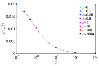
Figure 16: Empirical fit for $\varphi_{0}\left(\beta\right)$ as a function of $\beta$ for different vaues of $\beta$. (Left) Three dimensions, $256^{3}$ grid. (Right) Two dimensions, $512^{2}$ grid.

For $r>0.1h$ we introduce normalized functions $\tilde{f}_{\beta}$ and $\tilde{g}_{\beta}$ via

$$f_{\beta}(r) = -\frac{\beta}{2\pi\eta x^{2}}\cdot\tilde{f}_{\beta}(x),$$ (41)

$$g_{\beta}(r) = \frac{\beta}{\pi\eta x^{2}}\cdot\tilde{g}_{\beta}(x),$$

where in the inviscid case we take $\beta/\eta=\Delta t/\rho h^{2}$, and $x=r/h$ is the normalized distance. For finite $\beta$, we know that $\tilde{f}_{\beta}(x\gg\sqrt{\beta})\approx\tilde{g}_{\beta}(x\gg\sqrt{\beta})\approx 1$ according to (37). The numerical data is fitted with the empirical fitting functions

$$\tilde{f}_{\beta}(x) = \frac{x^{3}\ln(x)}{\beta(a_{0}+2x)}e^{-\frac{p_{1}x}{\sqrt{\beta}}}+\frac{a_{1}x^{2}+a_{2}x^{3}+a_{3}x^{4}}{1+b_{1}x^{2}+b_{2}x^{3}+a_{3}x^{4}},$$ (42)

$$\tilde{g}_{\beta}(x) = \frac{x^{3}}{\beta(c_{0}+4x)}e^{-\frac{p_{2}x}{\sqrt{\beta}}}+\frac{x^{3}}{e^{-p_{3}x}(c_{1}+c_{2}x+c_{3}x^{2})+x^{3}},$$

as shown in Fig. 17. Here $a_{0}-a_{3},\ p_{1}-p_{3},\ b_{1}-b_{3},\ c_{0}-c_{3}$ are empirical coefficients, computed by fitting numerical dats for $\beta$ in $\{0,\ 0.1,\ 0.25,\ 0.5,\ 1.0,\ 5.0,\ 10.0\}$. Intermediate values in the range $0<\beta<10.0$ are interpolated using linear interpolation, and larger $\beta$’s are handled using the steady Stokes fit (39).

Figure 17: Empirical fitting of $\tilde{f}_{\beta}(r)$ and $\tilde{g}_{\beta}(r)$ in two dimensions for different values of $\beta$ for the 6-point kernel, $512^{2}$ grid.

Appendix C Stokes flow between two concentric spheres

Consider steady Stokes flow around a rigid shell or sphere of radius $a$, placed in a centered position inside another spherical shell or cavity of radius $b=a/\lambda$. We consider the case when the outer shell is moving with velocity $V$ and the inner shell is at rest, and for simplicity set the viscosity to unity, $\eta=1$. Brenner BrennerBook gives the drag force on the inner sphere for no slip boundary conditions as

$$F=-6\pi aVK,$$ (43)

where

$$K=\frac{1-\lambda^{5}}{\alpha}\text{ and }\alpha={1-\frac{9}{4}\lambda+\frac{5}{2}\lambda^{3}-\frac{9}{4}\lambda^{5}+\lambda^{6}}.$$

Let us denote the constants

$$A = -\frac{15V}{4a^{2}}\cdot\frac{\lambda^{3}-\lambda^{5}}{\alpha},$$

$$B = \frac{3Va}{2}\cdot\frac{1-\lambda^{5}}{\alpha},$$

$$C = \frac{V}{2}\cdot\frac{1+\frac{5}{4}\lambda^{3}-\frac{9}{4}\lambda^{5}}{\alpha},$$

$$D = \frac{Va^{3}}{4}\cdot\frac{1-\lambda^{3}}{\alpha}.$$

The velocity in the region between the two spherical shells can be obtained from the expressions given by Brenner as

$$v_{r}=-\cos\theta\left(\frac{A}{5}r^{2}-B\frac{1}{r}+2C+2D\frac{1}{r^{3}}\right),$$

$$v_{\theta}=\sin\theta\left(\frac{A}{5}r^{2}-\frac{B}{2}\frac{1}{r}+2C-D\frac{1}{r^{3}}\right),$$

$$v_{\phi}=0,$$

and the pressure is

$$\pi=\pi_{\infty}+\mu B\frac{\cos\theta}{r^{2}}-2\mu Ar\cos\theta,$$

where $\pi_{\infty}=0$ since we impose that the pressure have mean zero to remove the null mode for pressure. In spherical coordinates, with the symmetry axes aligned with the direction of the flow, the traction on the surface of the inner sphere, which is the jump in the stress across the inner shell, is

$$\boldsymbol{\lambda}=\boldsymbol{\sigma}\cdot\boldsymbol{n} = \mu\cos\theta\left(2Ar-\frac{B}{r^{2}}\right)\hat{\boldsymbol{r}}+\mu\sin\theta\left(Ar+\frac{B}{r^{2}}\right)\hat{\boldsymbol{\theta}},$$

where $\hat{\boldsymbol{r}}=(\sin\theta\cos\phi,\quad\sin\theta\sin\phi,\quad\cos\theta)$ and $\hat{\boldsymbol{\theta}}=(\cos\theta\cos\phi,\;\cos\theta\sin\phi,\;-\sin\theta)$.

Appendix D Imposing Physical Boundary Conditions

The local averaging and spreading operators have to be modified near physical boundaries, specifically, when the support of the kernel $\delta_{a}$ overlaps with a boundary. A proposal for how to do that has been developed by Yeo and Maxey ForceCoupling_Channel , and an alternative proposal has been developed in the context of the immersed boundary method by Griffith et al. IBMDelta_Boundary . Here we have chosen to use the former approach because of its simplicity and the fact that it is independent of the kernel, as well as the fact that it ensures that the interpolated velocity strictly vanishes at a no-slip boundary; this ensures that the mobility of a marker is a monotonically decreasing function as it approaches a no-slip boundary. Since the description in ForceCoupling_Channel is limited to steady Stokes flow and a single no-slip boundary, we give here an algebraic formulation that extends to a variety of boundary conditions; this formulation is implemented in the IBAMR library and used in the examples in this paper in non-periodic domains.

The basic idea in the handling spreading and interpolation near boundaries is to use the standard IB kernel functions in a domain extended with sufficiently many ghost cells so that the support of all kernels is strictly within the extended domain. For interpolation, we first fill ghost cells and then interpolate as usual using the ghost cell values. For spreading, we take the adjoint operator, which basically means that we first spread to the extended domain including ghost cells in the usual manner, and then we accumulate the value spread to the ghost cell in the corresponding interior grid point, using the same weight (coefficient) that was used when filling ghost cells for the purposes of interpolation.

This process requires a consistent method for filling ghost cells, that is, for extending a (cell-centered or staggered) field $\boldsymbol{u}$ from the interior to the extended domain. In general, this will be an affine linear mapping of the form

$$\boldsymbol{u}_{\text{ext}}=\boldsymbol{E}\boldsymbol{u}_{\text{int}}+\boldsymbol{c},$$

where $\boldsymbol{E}$ is an extension matrix and $\boldsymbol{c}$ encodes inhomogeneous boundary conditions. Let us denote with $\boldsymbol{\mathcal{J}}_{0}$ the standard IB interpolation operator that interpolates an extended field at a position inside the interior of the domain. The interpolated value in the presence of physical boundary conditions is then given by the affine linear mapping

$$\boldsymbol{\mathcal{J}}_{BC}\left(\boldsymbol{u}_{\text{int}}\right)=\boldsymbol{\mathcal{J}}_{0}\boldsymbol{u}_{\text{ext}}=\boldsymbol{\mathcal{J}}_{0}\boldsymbol{E}\boldsymbol{u}_{\text{int}}+\boldsymbol{\mathcal{J}}_{0}\boldsymbol{c}.$$

The corresponding spreading operation is defined to be the adjoint of $\boldsymbol{\mathcal{J}}_{BC}$ for homogeneous boundary conditions, as this ensures energy conservation in the absence of boundary forcing. Specifically, we use

$$\boldsymbol{\mathcal{S}}_{BC}=\boldsymbol{E}^{T}\boldsymbol{\mathcal{J}}_{0}^{\star}=\boldsymbol{E}^{T}\boldsymbol{\mathcal{S}}_{0}.$$

The specific form of the extension operator $\boldsymbol{E}$ used in our implementation is based on linear extrapolation to a given ghost point based on the corresponding value in the interior and the values at the boundary as specified in the boundary conditions. Specifically, for homogeneous Neumann conditions we do a mirror image $u_{\text{ghost}}=-u_{\text{\text{int}}}$, while for homogeneous Dirichlet boundary conditions, such as no slip boundaries, we simply do a mirror inversion $u_{\text{ghost}}=-u_{\text{\text{int}}}$. This makes our implementation exactly identical to that proposed by Yeo and Maxey ForceCoupling_Channel in the context of the FCM method. One can think of this approach to no-slip boundaries as taking an inverted mirror image of the portion of the kernel outside of the domain ForceCoupling_Channel . Note that the same $\boldsymbol{E}$ is used to implement boundary conditions both in the fluid solver and when interpolating/spreading near boundaries; this greatly simplifies the implementation without lowering the second-order accuracy of the fluid solver NonProjection_Griffith . In our implementation, we use simple transpose for spreading which is the adjoint $\boldsymbol{E}^{\star}$ with respect to the standard inner product.

References

- (1) M. Uhlmann. An immersed boundary method with direct forcing for the simulation of particulate flows. J. Comp. Phys., 209(2):448–476, 2005.
- (2) A. P. S. Bhalla, R. Bale, B. E. Griffith, and N. A. Patankar. A unified mathematical framework and an adaptive numerical method for fluid-structure interaction with rigid, deforming, and elastic bodies. Journal of Computational Physics, 250:446–476, 2013.
- (3) K. Taira and T. Colonius. The immersed boundary method: a projection approach. J. Comp. Phys., 225(2):2118–2137, 2007.
- (4) Calvin Zhang, Robert D Guy, Brian Mulloney, Qinghai Zhang, and Timothy J Lewis. Neural mechanism of optimal limb coordination in crustacean swimming. Proceedings of the National Academy of Sciences, 111(38):13840–13845, 2014.
- (5) Shen-Wei Su, Ming-Chih Lai, and Chao-An Lin. An immersed boundary technique for simulating complex flows with rigid boundary. Computers & fluids, 36(2):313–324, 2007.
- (6) C.S. Peskin. The immersed boundary method. Acta Numerica, 11:479–517, 2002.
- (7) Joseph M Teran and Charles S Peskin. Tether force constraints in stokes flow by the immersed boundary method on a periodic domain. SIAM Journal on Scientific Computing, 31(5):3404–3416, 2009.
- (8) David B Stein, Robert D Guy, and Becca Thomases. Immersed boundary smooth extension: A high-order method for solving pde on arbitrary smooth domains using fourier spectral methods. Journal of Computational Physics, 304:252–274, 2016.
- (9) O. M. Curet, I. K. AlAli, M. A. MacIver, and N. A. Patankar. A versatile implicit iterative approach for fully resolved simulation of self-propulsion. Computer Methods in Applied Mechanics and Engineering, 199:2417–2424, 2010.
- (10) Arezoo Motavalizadeh Ardekani, Sadegh Dabiri, and Roger H Rangel. Collision of multi-particle and general shape objects in a viscous fluid. Journal of Computational Physics, 227(24):10094–10107, 2008.
- (11) S.V. Patankar. Numerical heat transfer and fluid flow. Hemisphere Pub, 1980.
- (12) T.T. Bringley and C.S. Peskin. Validation of a simple method for representing spheres and slender bodies in an immersed boundary method for Stokes flow on an unbounded domain. J. Comp. Phys., 227(11):5397–5425, 2008.
- (13) Matthias Heil, Andrew L Hazel, and Jonathan Boyle. Solvers for large-displacement fluid–structure interaction problems: segregated versus monolithic approaches. Computational Mechanics, 43(1):91–101, 2008.
- (14) MW Gee, U Küttler, and WA Wall. Truly monolithic algebraic multigrid for fluid–structure interaction. International Journal for Numerical Methods in Engineering, 85(8):987–1016, 2011.
- (15) A. Sierou and J. F. Brady. Accelerated Stokesian Dynamics simulations. J. Fluid Mech., 448:115–146, 2001.
- (16) James W Swan, John F Brady, Rachel S Moore, et al. Modeling hydrodynamic self-propulsion with Stokesian Dynamics. Or teaching Stokesian Dynamics to swim. Physics of Fluids, 23:071901, 2011.
- (17) K Hinsen. HYDROLIB: a library for the evaluation of hydrodynamic interactions in colloidal suspensions. Computer physics communications, 88(2):327–340, 1995.
- (18) B Cichocki and K Hinsen. Stokes drag on conglomerates of spheres. Physics of Fluids, 7:285, 1995.
- (19) A Ortega, D Amorós, and J García de La Torre. Prediction of hydrodynamic and other solution properties of rigid proteins from atomic-and residue-level models. Biophysical journal, 101(4):892–898, 2011. Code available at http://leonardo.inf.um.es/macromol/programs/hydropro/hydropro.htm.
- (20) José García de la Torre, María L Huertas, and Beatriz Carrasco. Calculation of hydrodynamic properties of globular proteins from their atomic-level structure. Biophysical Journal, 78(2):719–730, 2000.
- (21) Ricardo Cortez, Lisa Fauci, and Alexei Medovikov. The method of regularized Stokeslets in three dimensions: analysis, validation, and application to helical swimming. Physics of Fluids, 17:031504, 2005.
- (22) Ricardo Cortez. The method of regularized stokeslets. SIAM Journal on Scientific Computing, 23(4):1204–1225, 2001.
- (23) Ricardo Cortez, Bree Cummins, Karin Leiderman, and Douglas Varela. Computation of three-dimensional brinkman flows using regularized methods. Journal of Computational Physics, 229(20):7609–7624, 2010.
- (24) Yu Zhang, Juan J de Pablo, and Michael D Graham. An immersed boundary method for brownian dynamics simulation of polymers in complex geometries: Application to dna flowing through a nanoslit with embedded nanopits. The Journal of Chemical Physics, 136:014901, 2012.
- (25) Richard M Jendrejack, David C Schwartz, Michael D Graham, and Juan J de Pablo. Effect of confinement on DNA dynamics in microfluidic devices. J. Chem. Phys., 119:1165, 2003.
- (26) James W. Swan and John F. Brady. Simulation of hydrodynamically interacting particles near a no-slip boundary. Physics of Fluids, 19(11):113306, 2007.
- (27) James W Swan and John F Brady. Particle motion between parallel walls: Hydrodynamics and simulation. Physics of Fluids, 22:103301, 2010.
- (28) James W Swan and John F Brady. The hydrodynamics of confined dispersions. Journal of Fluid Mechanics, 687:254, 2011.
- (29) Anthony JC Ladd, Rahul Kekre, and Jason E Butler. Comparison of the static and dynamic properties of a semiflexible polymer using lattice Boltzmann and Brownian-dynamics simulations. Physical Review E, 80(3):036704, 2009.
- (30) Josephine Ainley, Sandra Durkin, Rafael Embid, Priya Boindala, and Ricardo Cortez. The method of images for regularized stokeslets. Journal of Computational Physics, 227(9):4600–4616, 2008.
- (31) Karin Leiderman, Elizabeth L Bouzarth, Ricardo Cortez, and Anita T Layton. A regularization method for the numerical solution of periodic stokes flow. Journal of Computational Physics, 236:187–202, 2013.
- (32) B.E. Griffith. An accurate and efficient method for the incompressible Navier-Stokes equations using the projection method as a preconditioner. J. Comp. Phys., 228(20):7565–7595, 2009.
- (33) M. Cai, A. J. Nonaka, J. B. Bell, B. E. Griffith, and A. Donev. Efficient Variable-Coefficient Finite-Volume Stokes Solvers. Comm. in Comp. Phys. (CiCP), 16(5):1263–1297, 2014.
- (34) S. Lomholt and M.R. Maxey. Force-coupling method for particulate two-phase flow: Stokes flow. J. Comp. Phys., 184(2):381–405, 2003.
- (35) F. Balboa Usabiaga, R. Delgado-Buscalioni, B. E. Griffith, and A. Donev. Inertial Coupling Method for particles in an incompressible fluctuating fluid. Comput. Methods Appl. Mech. Engrg., 269:139–172, 2014. Code available at https://code.google.com/p/fluam.
- (36) Somdeb Ghose and R Adhikari. Irreducible representations of oscillatory and swirling flows in active soft matter. Physical review letters, 112(11):118102, 2014.
- (37) Donald L Koch and Ganesh Subramanian. Collective hydrodynamics of swimming microorganisms: Living fluids. Annual Review of Fluid Mechanics, 43:637–659, 2011.
- (38) S. Delong, F. Balboa Usabiaga, R. Delgado-Buscalioni, B. E. Griffith, and A. Donev. Brownian Dynamics without Green’s Functions. J. Chem. Phys., 140(13):134110, 2014. Software available at https://github.com/stochasticHydroTools/FIB.
- (39) Eric E. Keaveny. Fluctuating force-coupling method for simulations of colloidal suspensions. J. Comp. Phys., 269(0):61 – 79, 2014.
- (40) P. J. Atzberger. Stochastic Eulerian-Lagrangian Methods for Fluid-Structure Interactions with Thermal Fluctuations. J. Comp. Phys., 230:2821–2837, 2011.
- (41) Amneet Pal Singh Bhalla, Rahul Bale, Boyce E. Griffith, and Neelesh A. Patankar. Fully resolved immersed electrohydrodynamics for particle motion, electrolocation, and self-propulsion. Journal of Computational Physics, 256:88 – 108, 2014.
- (42) B.E. Griffith, R.D. Hornung, D.M. McQueen, and C.S. Peskin. An adaptive, formally second order accurate version of the immersed boundary method. J. Comput. Phys., 223(1):10–49, 2007. Software available at http://ibamr.googlecode.com.
- (43) B.E. Griffith. Immersed boundary model of aortic heart valve dynamics with physiological driving and loading conditions. Int J Numer Meth Biomed Eng, 28:317–345, 2012.
- (44) B.E. Griffith. On the volume conservation of the immersed boundary method. Commun. Comput. Phys., 12:401–432, 2012.
- (45) Charles S Peskin and Beth Feller Printz. Improved volume conservation in the computation of flows with immersed elastic boundaries. Journal of computational physics, 105(1):33–46, 1993.
- (46) Boyce E Griffith and Xiaoyu Luo. Hybrid finite difference/finite element version of the immersed boundary method. Submitted in revised form, 2012.
- (47) Y. X. Bao, C. S. Peskin, B. Griffith, D. McQueen, and A. Donev. C. S. Peskin. In preparation, 2016.
- (48) Y. X. Bao, J. Kaye, and C. S. Peskin. A Gaussian-Like Immersed Boundary Kernel with Three Continuous Derivatives and Improved Translational Invariance. Preprint ArXiv:1505.07529. Software available at https://github.com/stochasticHydroTools/IBMethod, 2015.
- (49) HC Brinkman. A calculation of the viscous force exerted by a flowing fluid on a dense swarm of particles. Applied Scientific Research, 1(1):27–34, 1949.
- (50) A. Pal Singh Bhalla, B. E. Griffith, N. A. Patankar, and A. Donev. A Minimally-Resolved Immersed Boundary Model for Reaction-Diffusion Problems. J. Chem. Phys., 139(21):214112, 2013.
- (51) Reghan J Hill, Donald L Koch, and Anthony JC Ladd. Moderate-reynolds-number flows in ordered and random arrays of spheres. Journal of Fluid Mechanics, 448:243–278, 2001.
- (52) Donald L Koch and Anthony JC Ladd. Moderate reynolds number flows through periodic and random arrays of aligned cylinders. Journal of Fluid Mechanics, 349:31–66, 1997.
- (53) A.J.C. Ladd. Numerical simulations of particulate suspensions via a discretized Boltzmann equation. II. Numerical results. Journal of Fluid Mechanics, 271(1):311–339, 1994.
- (54) Howard Elman, Victoria E Howle, John Shadid, Robert Shuttleworth, and Ray Tuminaro. Block preconditioners based on approximate commutators. SIAM Journal on Scientific Computing, 27(5):1651–1668, 2006.
- (55) H.D. Ceniceros and J.E. Fisher. A fast, robust, and non-stiff Immersed Boundary Method. J. Comp. Phys., 230(12):5133 – 5153, 2011.
- (56) L Durlofsky and JF Brady. Analysis of the brinkman equation as a model for flow in porous media. Physics of Fluids, 30(11):3329–3341, 1987.
- (57) Jens Rotne and Stephen Prager. Variational treatment of hydrodynamic interaction in polymers. The Journal of Chemical Physics, 50:4831, 1969.
- (58) Zhi Liang, Zydrunas Gimbutas, Leslie Greengard, Jingfang Huang, and Shidong Jiang. A fast multipole method for the rotne–prager–yamakawa tensor and its applications. Journal of Computational Physics, 234:133–139, 2013.
- (59) Eligiusz Wajnryb, Krzysztof A Mizerski, Pawel J Zuk, and Piotr Szymczak. Generalization of the rotne–prager–yamakawa mobility and shear disturbance tensors. Journal of Fluid Mechanics, 731:R3, 2013.
- (60) Alexandre M Roma, Charles S Peskin, and Marsha J Berger. An adaptive version of the immersed boundary method. J. Comput. Phys., 153(2):509–534, 1999.
- (61) Satish Balay, William D. Gropp, Lois Curfman McInnes, and Barry F. Smith. Efficient management of parallelism in object oriented numerical software libraries. In E. Arge, A. M. Bruaset, and H. P. Langtangen, editors, Modern Software Tools in Scientific Computing, pages 163–202. Birkhäuser Press, 1997. Software available at http://www.mcs.anl.gov/petsc.
- (62) Howard C Elman, David J Silvester, and Andrew J Wathen. Finite elements and fast iterative solvers: with applications in incompressible fluid dynamics. Oxford University Press, 2014.
- (63) Xiaolei Yang, Xing Zhang, Zhilin Li, and Guo-Wei He. A smoothing technique for discrete delta functions with application to immersed boundary method in moving boundary simulations. Journal of Computational Physics, 228(20):7821–7836, 2009.
- (64) Reghan J Hill, Donald L Koch, and Anthony JC Ladd. The first effects of fluid inertia on flows in ordered and random arrays of spheres. Journal of Fluid Mechanics, 448:213–241, 2001.
- (65) F. Balboa Usabiaga, I. Pagonabarraga, and R. Delgado-Buscalioni. Inertial coupling for point particle fluctuating hydrodynamics. J. Comp. Phys., 235:701–722, 2013.
- (66) Adolfo Vazquez-Quesada, Florencio Balboa Usabiaga, and Rafael Delgado-Buscalioni. A multiblob approach to colloidal hydrodynamics with inherent lubrication. The Journal of Chemical Physics, 141(20), 2014.
- (67) H Hasimoto. On the periodic fundamental solutions of the stokes equations and their application to viscous flow past a cubic array of spheres. J. Fluid Mech, 5(02):317–328, 1959.
- (68) Harvey AR Williams, Lisa J Fauci, and Donald P Gaver III. Evaluation of interfacial fluid dynamical stresses using the immersed boundary method. Discrete and continuous dynamical systems. Series B, 11(2):519, 2009.
- (69) Rahul Kekre, Jason E. Butler, and Anthony J. C. Ladd. Comparison of lattice-Boltzmann and Brownian-dynamics simulations of polymer migration in confined flows. Phys. Rev. E, 82:011802, 2010.
- (70) Oana Marin, Katarina Gustavsson, and Anna-Karin Tornberg. A highly accurate boundary treatment for confined stokes flow. Computers & Fluids, 66:215–230, 2012.
- (71) S Bhattacharya, J Blawzdziewicz, and E Wajnryb. Hydrodynamic interactions of spherical particles in suspensions confined between two planar walls. Journal of Fluid Mechanics, 541:263–292, 2005.
- (72) Ludvig Af Klinteberg and Anna-Karin Tornberg. Fast ewald summation for stokesian particle suspensions. International Journal for Numerical Methods in Fluids, 76(10):669–698, 2014.
- (73) Sofiane Benyahia, Madhava Syamlal, and Thomas J O’Brien. Extension of hill–koch–ladd drag correlation over all ranges of reynolds number and solids volume fraction. Powder Technology, 162(2):166–174, 2006.
- (74) J. P. Hernandez-Ortiz, J. J. de Pablo, and M. D. Graham. Fast Computation of Many-Particle Hydrodynamic and Electrostatic Interactions in a Confined Geometry. Phys. Rev. Lett., 98(14):140602, 2007.
- (75) Shidong Jiang, Zhi Liang, and Jingfang Huang. A fast algorithm for brownian dynamics simulation with hydrodynamic interactions. Mathematics of Computation, 82(283):1631–1645, 2013.
- (76) Constantine Pozrikidis. Boundary integral and singularity methods for linearized viscous flow. Cambridge University Press, 1992.
- (77) Sivaram Ambikasaran and Eric Darve. An fast direct solver for partial hierarchically semi-separable matrices. Journal of Scientific Computing, 57(3):477–501, 2013.
- (78) Kenneth L Ho and Leslie Greengard. A fast direct solver for structured linear systems by recursive skeletonization. SIAM Journal on Scientific Computing, 34(5):A2507–A2532, 2012.
- (79) Amirhossein Aminfar, Sivaram Ambikasaran, and Eric Darve. A fast block low-rank dense solver with applications to finite-element matrices. Journal of Computational Physics, 304:170 – 188, 2016.
- (80) Pieter Coulier, Hadi Pouransari, and Eric Darve. The inverse fast multipole method: using a fast approximate direct solver as a preconditioner for dense linear systems. arXiv preprint arXiv:1508.01835, 2015.
- (81) E.P. Newren, A.L. Fogelson, R.D. Guy, and R.M. Kirby. A comparison of implicit solvers for the immersed boundary equations. Computer Methods in Applied Mechanics and Engineering, 197(25-28):2290–2304, 2008.
- (82) Robert D Guy and Bobby Philip. A multigrid method for a model of the implicit immersed boundary equations. Communications in Computational Physics, 12(2):378, 2012.
- (83) Qinghai Zhang, Robert D Guy, and Bobby Philip. A projection preconditioner for solving the implicit immersed boundary equations. Numer. Math. Theor. Meth. Appl.(Special issue on Fluid Structure Interactions), 7(4):473–498, 2014.
- (84) C. W. J. Beenakker. Ewald sum of the Rotne-Prager tensor. J. Chem. Phys., 85:1581, 1986.
- (85) John Happel and Howard Brenner. Low Reynolds number hydrodynamics: with special applications to particulate media, volume 1. Springer Science & Business Media, 1983.
- (86) Kyongmin Yeo and Martin R Maxey. Dynamics of concentrated suspensions of non-colloidal particles in couette flow. Journal of Fluid Mechanics, 649(1):205–231, 2010.
- (87) B.E. Griffith, X. Luo, D.M. McQueen, and C.S. Peskin. Simulating the fluid dynamics of natural and prosthetic heart valves using the immersed boundary method. International Journal of Applied Mechanics, 1(01):137–177, 2009.