Angular momentum in spin-phonon processes

Abstract

Quantum theory of spin relaxation in the elastic environment is revised with account of the concept of a phonon spin recently introduced by Zhang and Niu (PRL 2014). Similar to the case of the electromagnetic field, the division of the angular momentum associated with elastic deformations into the orbital part and the part due to phonon spins proves to be useful for the analysis of the balance of the angular momentum. Such analysis sheds important light on microscopic processes leading to the Einstein - de Haas effect.

I Introduction

The problem of conservation of angular momentum in systems containing magnetic moments has been around since the discovery of Einstein - de Haas EdH and Barnett Barnett effects one hundred years ago. The first effect demonstrated that the change in the magnetic moment of a feely suspended body generates mechanical rotation, while the second demonstrated that mechanical rotation induces magnetization. For some time the Einstein - de Haas and Barnett effects were used to measure the gyromagnetic ratio of solids Bar-Scott . The significance of such measurements was diminished by the discovery of the electron spin resonance and the ferromagnetic resonance that provided a more accurate determination of the gyromagnetic ratio. After that the experiments on macroscopic magneto-mechanical gyroscopic effects have been largely abandoned. Surprisingly, however, microscopic mechanisms of the transfer of the spin angular momentum to the phonon system and subsequently to the body as a whole remain poorly understood.

The tradition that goes back to the pioneering work on spin-phonon relaxation by Van Vleck VanVleck-PR40 consists of ignoring conservation of angular momentum under the excuse that the Hamiltonian of the system does not possess full rotational invariance. It is clear, however, that in theory (and in experiment) the angular momentum in a system of interacting spins and phonons is conserved. This prompted a significant effort by a number of researchers to formulate the theory of magneto-elastic interactions in a rotationally invariant manner mel72prl ; dohful75 ; fed75prb ; bonmel76prb ; fedmel76prb ; fed77prb ; chugarsch05prb . The advantage of such approach is that it is parameter free in a sense that spin-phonon rates can be expressed in terms of the well-known independently measured parameters.

Emergence of micro- and nanoelectromechanical devices (MEMS and NEMS) rejuvinated interest to the problem of angular momentum in magneto-mechanical systems chugar14prb . Einstein - de Haas effect at the nanoscale has been experimentally studied in magnetic microcantilevers walmorkab06apl ; limimtwal14epl and theoretically explained by the motion of domain walls jaachugar09prb . Switching of magnetic moments by mechanical torques in nanocantilevers has been proposed Kovalev-PRL2005 ; cai-PRA14 ; CJ-JAP2015 . Mechanical resonators containing single magnetic molecules have been studied by quantum methods jaachu09prl ; jaachugar10epl ; kovhaybau11prl ; carchu11prx ; okechugar13prb . Experiments have progressed to the measurement of the angular momentum exchange between of a single molecular spin and a carbon nanotube ganklyrub13NatNano ; ganklyrub13acsNano .

In nanoresonators the problem is somewhat simpler due to the finite number of resonant modes. For a single spin in a macroscopic body, however, the number of phonon degrees of freedom is practically infinite. In relation to the angular momentum this problem has received significant recent attention in experiments with atomic spin - based qubits Awschalom1 ; Awschalom2 and in application to spintronics Qin-PRB12 . To address this problem Zhang and Niu recently introduced a concept of the phonon spin Zhang-Niu .

In this paper we investigate this concept for the process of the relaxation of a single atomic spin in a macroscopic body. By developing an approach similar to that for photons we find that within the elastic theory the angular momentum of phonons can be naturally split into the orbital angular momentum ${\bf L}^{(1)}$ and the spin angular momentum ${\bf L}^{(2)}$. The orbital part corresponds to the rotation of the elastic medium around a certain point, while the spin part corresponds to a small-radius circular shear displacements of points of the elastic media around their equilibrium positions, see Fig. 1.

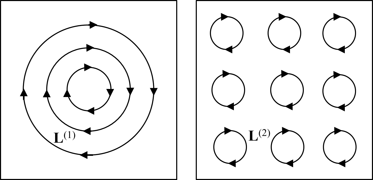
Figure 1: Conceptual representation of the motion of the elastic medium that generates the orbital angular momentum ${\bf L}^{(1)}$ and the phonon spin angular momentum ${\bf L}^{(2)}$.

The paper is structured as follows. The concept of the angular momentum in classical and quantum theories of elasticity is discussed in Section II. Conservation of the total angular momentum is studied in Section III by computing its commutator with the Hamiltonian. Quantum dynamics of the angular momentum of the relaxing spin and emitted phonons is investigated in Section IV. Section V contains summary of the results and some final comments.

II The angular momentum

II.1 Angular momentum in the classical theory of elasticity

The angular momentum of the elastic solid is defined as

$$\mathbf{L}=\int d^{3}r\left(\mathbf{r}+\mathbf{u}\right)\times\mathbf{p},$$ (1)

where time-indendent $\mathbf{r}$ corresponds to the non-deformed body, $\mathbf{u}({\bf r},t)$ is deformation, and $\mathbf{p}({(\bf r},t)=\rho\dot{\bf u}({(\bf r},t)$ is the momentum density. It consists of two parts

$${\bf L}={\bf L}^{(1)}+{\bf L}^{(2)},$$ (2)

where

$${\bf L}^{(1)}=\int d^{3}r\rho\,\mathbf{r}\times\dot{\bf u},\quad{\bf L}^{(2)}=\int d^{3}r\rho\,\mathbf{u}\times\dot{\bf u}.$$ (3)

The orbital part described by ${\bf L}^{(1)}$ corresponds to the rotation of the elastic medium around the origin, while the spin part described by ${\bf L}^{(2)}$ corresponds to a small-radius circular shear displacements of points of the elastic media around their equilibrium positions, see Fig. 1.

Applying time derivative to these expressions one obtains

$$\dot{\bf L}^{(1)}=\int d^{3}r\rho\,{\bf r}\times\ddot{\bf u},\quad\dot{\bf L}^{(2)}=\int d^{3}r\rho\,{\bf u}\times\ddot{\bf u}.$$ (4)

The dynamical equation for the displacement field is the Newton’s equation

$$\rho\frac{\partial^{2}u_{\alpha}}{\partial t^{2}}=\frac{\partial\sigma_{\alpha\beta}}{\partial r_{\beta}}$$ (5)

with the force in the right-hand-side being a gradient of the stress tensor $\sigma_{\alpha\beta}={\delta H}/{\delta e_{\alpha\beta}}$. Here $H$ is the Hamiltonian of the system and $e_{\alpha\beta}={\partial u_{\alpha}}/{\partial r_{\beta}}$. After integrating by parts in equations (4) and assuming zero elastic stress at the boundary of the body, one obtains

$$\dot{L}_{\alpha}^{(1)}=-\int d^{3}r\epsilon_{\alpha\beta\gamma}\sigma_{\gamma\beta},\quad\dot{L}_{\alpha}^{(2)}=-\int d^{3}r\epsilon_{\alpha\beta\gamma}e_{\beta\delta}\sigma_{\gamma\delta}$$ (6)

In the linear elastic theory $\dot{\bf L}^{(1)}$ is zero in the absence of internal torques due to the symmetry of the stress tensor. Such torques are ignored by the conventional elastic theory. ${\bf L}^{(2)}$, that is quadratic on deformations, is also neglected in the linear elastic theory, making $\dot{\bf L}=0$.

When $\sigma_{\alpha\beta}$ is non-symmetric, more care is needed. This can happen for two reasons. The first reason is the intrinsic anharmonicity of the elastic theory due to the nonlinearity of the strain tensor LL-elasticity ,

$$u_{\rho\eta}=\frac{1}{2}\left(e_{\rho\eta}+e_{\eta\rho}+e_{\nu\rho}e_{\nu\eta}\right)$$ (7)

The fact that $H$ must depend on $u_{\rho\eta}$ leads to

$$\sigma_{\gamma\delta}=\frac{\delta H}{\delta e_{\gamma\delta}}=\frac{\delta u_{\rho\eta}}{\delta e_{\gamma\delta}}\frac{\delta{H}}{\delta u_{\rho\eta}}=\frac{\delta{H}}{\delta u_{\gamma\delta}}+e_{\gamma\rho}\frac{\delta{H}}{\delta u_{\rho\delta}}$$ (8)

which is non-symmetric. It is easy to see that in this case the second term in Eq. (6) is needed for the condition $\dot{\bf L}=0$ to be exact.

Anharmonicity, however, is not the only reason for $\sigma_{\alpha\beta}$ to be non-symmetric. It also happens in the presence of spins because spin dynamics generates internal torques. Consider, e.g., a uniaxial spin Hamiltonian of the form

$$\hat{H}=-D\left(\mathbf{n\cdot S}\right)^{2}$$ (9)

with ${\bf n}$ being the magnetic anisotropy axis. Elastic deformations of the body rotate the anisotropy axis $\mathbf{n}$ by a small angle ${\bm{\phi}}$

$${\bm{\phi}}=\frac{1}{2}\nabla\times\mathbf{u}(\mathbf{r}),\quad\phi_{\alpha}=\frac{1}{2}\epsilon_{\alpha\beta\gamma}e_{\gamma\beta}.$$ (10)

To the first order in ${\bm{\phi}}$ one has $\mathbf{n}=\mathbf{e}_{z}+\left[{\bm{\phi}}\times\mathbf{e}_{z}\right]$. Expanding $\hat{H}$ up to the linear terms in $\phi$, we get $\hat{H}=\hat{H}_{A}+\hat{H}_{\mathrm{s-ph}}$, where $\hat{H}_{A}=-DS_{z}^{2}$ and the spin-lattice coupling is given by chugar97prb

$$\hat{H}_{\mathrm{s-ph}}=-D\left(S_{x}S_{z}+S_{z}S_{x}\right)\phi_{y}+D\left(S_{y}S_{z}+S_{z}S_{y}\right)\phi_{x}.$$ (11)

The corresponding stress tensor $\sigma_{\alpha\beta}={\delta H}_{\mathrm{s-ph}}/{\delta e_{\alpha\beta}}$ is non-symmetric. Writing it as

$$\sigma_{\alpha\beta}=\frac{\delta H_{\mathrm{s-ph}}}{\delta e_{\alpha\beta}}=\frac{\delta H_{\mathrm{s-ph}}}{\delta\phi_{\gamma}}\frac{\delta\phi_{\gamma}}{\delta e_{\alpha\beta}}$$ (12)

one obtains

$$\dot{\bf L}^{(1)}=-\int d^{3}r\frac{\delta H_{\mathrm{s-ph}}}{\delta{\bm{\phi}}},$$ (13)

which explicitly expresses the internal mechanical torque via the elastic twist. The latter comes from the spin-lattice coupling. In what follows we will show that ${\bf L}^{(2)}$ associated with the phonon spin is also generated in the problem of quantum relaxation of the atomic spin. Consequently, ${\bf L}^{(2)}$, that is usually neglected in the linear elastic theory, turns out to be important for the conservation of the total angular momentum, even in cases when the problem is solved with linear non-interacting phonons.

II.2 Quantum theory of phonon angular momentum

To obtain the second-quantized expression for the angular momentum, we use canonical quantization of phonons

$$\mathbf{u}(\mathbf{r})=\sqrt{\frac{\hbar}{2\rho V}}\sum_{\mathbf{k}\lambda}\frac{\mathbf{e}_{\mathbf{k}\lambda}e^{i\mathbf{k\cdot r}}}{\sqrt{\omega_{\mathbf{k}\lambda}}}a_{\mathbf{k}\lambda}+h.c.,$$ (14)

where $\rho$ is the mass density, $V$ is the volume, $\mathbf{e}_{\mathbf{k}\lambda}$ are polarization vectors, $\omega_{\mathbf{k}\lambda}$ are phonon frequencies and $a$, $a^{\dagger}$ are creation and annihilation operators of phonons. One uses Eq. (14), as well as

$$\mathbf{p}(\mathbf{r})=\rho\mathbf{\dot{u}}(\mathbf{r})=-i\sqrt{\frac{\rho\hbar}{2V}}\sum_{\mathbf{k}\lambda}\mathbf{e}_{\mathbf{k}\lambda}\sqrt{\omega_{\mathbf{k}\lambda}}e^{i\mathbf{k\cdot r}}a_{\mathbf{k}\lambda}+h.c.$$ (15)

The angular momentum of the body, Eq. (1), consists of two contributions, $\hat{\mathbf{L}}=\mathbf{\hat{L}}^{(1)}+\mathbf{\hat{L}}^{(2)}$ that have been discussed earlier. Here $\mathbf{\hat{L}}^{(1)}$ is first order in phonon operators and it can be interpreted as the orbital angular momentum of the phonons. The term $\mathbf{\hat{L}}^{(2)}$ is second-order in phonon operators and it can be interpreted as the spin of the phonons. Splitting the angular momentum into two parts is similar to that of photons. It will be shown below that the spin of a phonon is $\hbar$ and the phonon-spin eigenstates are circularly-polarized phonons.

The operator of the orbital angular momentum becomes

$$\mathbf{\hat{L}}^{(1)}=\sqrt{\frac{\rho\hbar}{2V}}\sum_{\mathbf{k}\lambda}\sqrt{\omega_{\mathbf{k}\lambda}}\left[\mathbf{e}_{\mathbf{k}\lambda}\times\mathbf{j}_{\mathbf{k}}\right]a_{\mathbf{k}\lambda}+h.c.,$$ (16)

where $\mathbf{j}_{\mathbf{k}}\equiv i\int d^{3}r\,\mathbf{r}e^{i\mathbf{k\cdot r}}$. As, by symmetry, $\mathbf{j}_{\mathbf{k}}$ can only be directed along $\mathbf{k}$, only transverse phonons contribute into $\mathbf{\hat{L}}^{(1)}$. In an infinite body, wave vectors are continuous, so that one can replace summation by integration

$$\frac{1}{V}\sum_{\mathbf{k}}\ldots\Rightarrow\int\frac{d^{3}k}{\left(2\pi\right)^{3}}\ldots$$ (17)

Then one can express $\mathbf{j}_{\mathbf{k}}$ as

$$\mathbf{j}_{\mathbf{k}}=\left(2\pi\right)^{3}\partial_{\mathbf{k}}\delta\left(\mathbf{k}\right).$$ (18)

Dropping the terms $aa$ and $a^{\dagger}a^{\dagger}$ in $\mathbf{\hat{L}}^{(2)}$ that do not conserve the number of phonon excitations, one obtains after integration over the volume

$$\mathbf{\hat{L}}^{(2)}=\frac{i\hbar}{2}\sum_{\mathbf{k}\lambda\lambda^{\prime}}\left[\mathbf{e}_{\mathbf{k}\lambda}\times\mathbf{e}_{\mathbf{k}\lambda^{\prime}}\right]a_{\mathbf{k}\lambda}a_{\mathbf{k}^{\prime}\lambda^{\prime}}^{\dagger}+h.c.$$ (19)

Keeping only transverse phonons, $\lambda\lambda^{\prime}=1,2$ and using $\left[\mathbf{e}_{\mathbf{k}1}\times\mathbf{e}_{\mathbf{k}2}\right]=\mathbf{k}/k$, one arrives at

$$\mathbf{\hat{L}}^{(2)}=i\hbar\sum_{\mathbf{k}}\frac{\mathbf{k}}{k}\left(a_{\mathbf{k}2}^{\dagger}a_{\mathbf{k}1}-a_{\mathbf{k}1}^{\dagger}a_{\mathbf{k}2}\right).$$ (20)

This operator becomes diagonal in terms of numbers of circularly-polarized phonons $a_{\mathbf{k}\pm}\equiv\left(a_{\mathbf{k}1}\pm ia_{\mathbf{k}2}\right)/\sqrt{2}$

$$\mathbf{\hat{L}}^{(2)}=\hbar\sum_{\mathbf{k}}\frac{\mathbf{k}}{k}\left(-a_{\mathbf{k}+}^{\dagger}a_{\mathbf{k}+}+a_{\mathbf{k}-}^{\dagger}a_{\mathbf{k}-}\right).$$ (21)

Each such phonon carries an angular momentum $\hbar$ parallel or anti-parallel to its wave vector that can be interpreted as the spin of the phonon.

In what follows we will study conservation of the angular momentum in the spin-relaxation model by computing its commutator with the Hamiltonian. Introducing spin operators $S_{\pm}\equiv S_{x}\pm iS_{y}$ that follow commutation relations $\left[S_{\pm},S_{z}\right]=\pm S_{\pm}$, one obtains from Eq. (11)

$$\hat{H}_{\mathrm{s-ph}}=-\frac{iD}{2}\left(S_{+}S_{z}+S_{z}S_{+}\right)\phi_{-}+h.c.,$$ (22)

where $\phi_{\pm}\equiv\phi_{x}\pm i\phi_{y}$. Using Eqs. (10) and (14) with the atomic spin located at $\mathbf{r}=0$, one obtains

$$\phi_{\pm}=\frac{1}{2}\sqrt{\frac{\hbar}{2\rho V}}\sum_{\mathbf{k}\lambda}\frac{\mathbf{e}_{\pm}\cdot\left[i\mathbf{k}\times\mathbf{e}_{\mathbf{k}\lambda}\right]}{\sqrt{\omega_{\mathbf{k}\lambda}}}\left(a_{\mathbf{k}\lambda}-a_{\mathbf{k}\lambda}^{\dagger}\right),$$ (23)

where $\mathbf{e}_{\pm}\equiv\mathbf{e}_{x}\pm i\mathbf{e}_{y}$.

III Conservation of the angular momentum

Let us now check conservation of the total angular momentum

$$\mathbf{J}=\mathbf{L}+\hbar\mathbf{S}$$ (24)

that implies that $\mathbf{J}$ must commute with the Hamiltonian. The dynamical change of the spin operator has to be absorbed by the angular momentum of the elastic matrix, whose evolution is given by

$$\hat{\dot{\mathbf{L}}}=\frac{i}{\hbar}\left[\hat{H}_{\mathrm{s-ph}},\mathbf{\hat{L}}\right].$$ (25)

In particular, the precession of the spin around the anisotropy axis creates the co-wiggling of the elastic matrix with the spin.

It turns out that by commuting operators one can prove conservation of some parts of the angular momentum, whereas the complete prove of conservation requires a full quantum-mechanical solution for the relaxing spin and phonons created by its precession, presented in the next section. The situation is different for the angular momentum components perpendicular and parallel to the anisotropy axis. We will need commutators

$$\left[\phi_{\pm},\mathbf{\hat{L}}^{(1)}\right]=i\frac{\hbar}{2V}\sum_{\mathbf{k}\lambda}\left(\mathbf{e}_{\pm}\cdot\left[\mathbf{k}\times\mathbf{e}_{\mathbf{k}\lambda}\right]\right)\left[\mathbf{e}_{\mathbf{k}\lambda}\times\mathbf{j}_{\mathbf{k}}\right]$$ (26)

and

$$\left[\phi_{\pm},\mathbf{\hat{L}}^{(2)}\right]=\frac{\hbar}{2}\sqrt{\frac{\hbar}{2\rho V}}\sum_{\mathbf{k}\lambda}\frac{\mathbf{k}}{\sqrt{\omega_{\mathbf{k}}}}\left(\mathbf{e}_{\pm}\cdot\mathbf{e}_{\mathbf{k}\lambda}\right)\left(a_{\mathbf{k}\lambda}-a_{\mathbf{k}\lambda}^{\dagger}\right)$$ (27)

that follow from Eqs. (23), (16), and (20).

Let us first consider dynamics of the transverse components of the angular momentum. The dominant source of spin precession around the anisotropy axis is the unperturbed spin Hamiltonian $\hat{H}_{A}$:

$$\dot{S}_{x}=\frac{i}{\hbar}\left[\hat{H}_{\mathrm{A}},S_{x}\right]=-\frac{i}{\hbar}D\left[S_{z}^{2},S_{x}\right]=\frac{D}{\hbar}\left(S_{z}S_{y}+S_{y}S_{z}\right).$$ (28)

For the matrix, let us first consider the dynamics of the phonon orbital angular momentum $\hat{\mathbf{L}}^{(1)}$. From Eq. (26) with the help of the identity

$$\sum_{\lambda=1,2}\left(\mathbf{e}_{\mathbf{k}\lambda}\cdot\mathbf{A}\right)\left(\mathbf{e}_{\mathbf{k}\lambda}\cdot\mathbf{B}\right)=\mathbf{A\cdot B}-\left(\frac{\mathbf{k}}{k}\cdot\mathbf{A}\right)\left(\frac{\mathbf{k}}{k}\cdot\mathbf{B}\right)$$ (29)

and Eq. (18) one obtains

$$\left[\phi_{\pm},\hat{L}_{x}^{(1)}\right] = i\frac{\hbar}{2V}\sum_{\mathbf{k}\lambda}\left(\mathbf{e}_{\pm}\cdot\left[\mathbf{k}\times\mathbf{e}_{\mathbf{k}\lambda}\right]\right)\left(\mathbf{e}_{x}\cdot\left[\mathbf{e}_{\mathbf{k}\lambda}\times\mathbf{j}_{\mathbf{k}}\right]\right)$$ (30)

$$= i\frac{\hbar}{2V}\sum_{\mathbf{k}\lambda}\left(\mathbf{e}_{\mathbf{k}\lambda}\cdot\left[\mathbf{e}_{\pm}\times\mathbf{k}\right]\right)\left(\mathbf{e}_{\mathbf{k}\lambda}\cdot\left[\mathbf{j}_{\mathbf{k}}\times\mathbf{e}_{x}\right]\right)$$

$$= i\frac{\hbar}{2V}\sum_{\mathbf{k}}\left[\mathbf{e}_{\pm}\times\mathbf{k}\right]\cdot\left[\mathbf{j}_{\mathbf{k}}\times\mathbf{e}_{x}\right]$$

$$= i\frac{\hbar}{2V}\sum_{\mathbf{k}}\left\{\left(\mathbf{e}_{\pm}\cdot\mathbf{j}_{\mathbf{k}}\right)\left(\mathbf{e}_{x}\cdot\mathbf{k}\right)-\left(\mathbf{e}_{\pm}\cdot\mathbf{e}_{x}\right)\left(\mathbf{k}\cdot\mathbf{j}_{\mathbf{k}}\right)\right\}$$

$$= i\frac{\hbar}{2}\int d^{3}k\left\{k_{x}\partial_{k_{x}}\delta\left(\mathbf{k}\right)-\left(\mathbf{k}\cdot\partial_{\mathbf{k}}\delta\left(\mathbf{k}\right)\right)\right\}$$

$$= i\hbar.$$

Now from Eqs. (25) and (22) one obtains

$$\hat{\dot{L}}_{x}^{(1)}=-D\left(S_{y}S_{z}+S_{z}S_{y}\right).$$ (31)

Combining this with Eq. (28), one obtains the conservation law

$$\hbar\dot{S}_{x}+\hat{\dot{L}}_{x}^{(1)}=0.$$ (32)

In the same way one can obtain $\hbar\dot{S}_{y}+\hat{\dot{L}}_{y}^{(1)}=0.$

However, Eq. (32) is not the whole story. One has to consider $\hat{\dot{L}}_{x,y}^{(2)}$ using Eqs. (27) and (22). The resulting expression is a sum over $\mathbf{k}$, linear in phonon operators. It is of the same order as the contribution to $\hbar\dot{S}_{x,y}$ due to the spin-phonon interaction, $i\left[\hat{H}_{\mathrm{s-ph}},S_{x,y}\right]$, that was ignored above. Both terms discussed here are much smaller than the dominant terms in the angular momentum, conserved according to Eq. (32). These small terms are related to the spin-lattice relaxation of the spin. It is impossible to prove conservation of these terms without performing the full quantum-mechanical solution of the problem of spin relaxation.

Considering dynamics of the longitudinal component of the angular momentum, one can prove

$$\dot{L}_{z}^{(1)}=\frac{i}{\hbar}\left[\hat{H}_{\mathrm{s-ph}},L_{z}^{(1)}\right]=0$$ (33)

by a calculation similar to that in Eq. (30). The terms $\dot{S}_{z}$ and $\dot{L}_{z}^{(2)}$ are related to spin-lattice relaxation and they are sums over $\mathbf{k}$, linear in phonon operators. However, one cannot prove

$$\hbar\dot{S}_{z}+\dot{L}_{z}^{(2)}=0$$ (34)

without the full solution of the quantum problem that will be presented below.

IV Quantum theory of the relaxing spin

IV.1 General solution

To facilitate solving the problem of spin-lattice relaxation, we reduce the spin-phonon Hamiltonian to the rotating-wave approximation (RWA) form that conserves the energy. Consider transitions of the spin $\left|m-1\right\rangle\rightarrow\left|m\right\rangle$ for $m>0$ decreasing its energy and call the spin states $\left|1\right\rangle$ and $\left|0\right\rangle$, respectively. With the help of Eq. (22) one obtains the spin matrix element of this transition

$$\left\langle m-1\left|\hat{H}_{\mathrm{s-ph}}\right|m\right\rangle=\frac{iD}{2}\left(2m-1\right)l_{m-1,m}\phi_{+},$$ (35)

where $l_{m-1,m}\equiv\sqrt{S\left(S+1\right)-m(m-1)}$. Using Eqs. (22) and (23), one obtains the RWA coupling in the form

$$\hat{V}=\sum_{\mathbf{k}\lambda}\left(A_{\mathbf{k}\lambda}^{\ast}X^{01}a_{\mathbf{k}\lambda}^{\dagger}+A_{\mathbf{k}\lambda}X^{10}a_{\mathbf{k}\lambda}\right),$$ (36)

where

$$A_{\mathbf{k}\lambda}\equiv-\frac{D}{4}\left(2m-1\right)l_{m-1,m}\sqrt{\frac{\hbar}{2\rho V}}\frac{\mathbf{e}_{+}\cdot\left[\mathbf{k}\times\mathbf{e}_{\mathbf{k}\lambda}\right]}{\sqrt{\omega_{\mathbf{k}\lambda}}}$$ (37)

and the $X$-operators are defined by

$$X^{01}\left|1\right\rangle=\left|0\right\rangle,\qquad X^{10}\left|0\right\rangle=\left|1\right\rangle.$$ (38)

The quantum state of the system can be specified by

$$\Psi=\left(cX^{10}+\sum_{\mathbf{k}\lambda}c_{\mathbf{k}\lambda}a_{\mathbf{k}\lambda}^{\dagger}\right)\left|00\right\rangle,$$ (39)

where $\left|00\right\rangle$ is the “vacuum” state. $\Psi$ has only one excitation, spin or phonon. Considering the excited state of the spin as the reference-energy state, one obtains the Schrödinger equation for the coefficients

$$\dot{c} = -\frac{i}{\hbar}\sum_{\mathbf{k}\lambda}A_{\mathbf{k}\lambda}c_{\mathbf{k}\lambda}$$

$$\dot{c}_{\mathbf{k}\lambda} = -i\left(\omega_{\mathbf{k}\lambda}-\omega_{0}\right)c_{\mathbf{k}\lambda}-\frac{i}{\hbar}A_{\mathbf{k}\lambda}^{\ast}c,$$ (40)

where $\omega_{0}\equiv\left(E_{1}-E_{0}\right)/\hbar$ is the frequency of the transition between the spin levels.

One can integrate the equations for the phonon modes $c_{\mathbf{k}}$ assuming the initial condition of the phonon vacuum:

$$c_{\mathbf{k}\lambda}(t) = -\frac{iA_{\mathbf{k}\lambda}^{\ast}}{\hbar}\int_{0}^{t}dt^{\prime}e^{-i\left(\omega_{\mathbf{k}\lambda}-\omega_{0}\right)(t-t^{\prime})}c(t^{\prime})$$ (41)

$$= -\frac{iA_{\mathbf{k}\lambda}^{\ast}}{\hbar}\int_{0}^{t}d\tau e^{-i\left(\omega_{\mathbf{k}\lambda}-\omega_{0}\right)\tau}c(t-\tau)$$

and insert the result into the equation for the spin $c$:

$$\frac{dc}{dt}=-\frac{1}{\hbar^{2}}\sum_{\mathbf{k}\lambda}\left|A_{\mathbf{k}\lambda}\right|^{2}\int_{0}^{t}d\tau e^{-i\left(\omega_{\mathbf{k}\lambda}-\omega_{0}\right)\tau}c(t-\tau).$$ (42)

In this integro-differential equation, $c(t-\tau)$ is a slow function of time, whereas the memory function $f(\tau)=\sum_{\mathbf{k}\lambda}\left|A_{\mathbf{k}\lambda}\right|^{2}e^{-i\left(\omega_{\mathbf{k}\lambda}-\omega_{0}\right)\tau}$ is sharply peaked at $\tau=0.$ Thus one can replace $c(t-\tau)\Rightarrow c(t),$ after which integration over $\tau$ and keeping only real contribution responsible for the relaxation yields the equation

$$\frac{dc}{dt}=-\frac{\Gamma}{2}c,$$ (43)

and thus

$$c=e^{-\left(\Gamma/2\right)t},$$ (44)

where

$$\Gamma=\frac{2\pi}{\hbar^{2}}\sum_{\mathbf{k}\lambda}\left|A_{\mathbf{k}\lambda}\right|^{2}\delta\left(\omega_{\mathbf{k}\lambda}-\omega_{0}\right)$$ (45)

is the spin relaxation rate. Now, adopting this solution in Eq. (41) and integrating over time, one obtains for the phonons

$$c_{\mathbf{k}\lambda}(t)=\frac{A_{\mathbf{k}\lambda}^{\ast}}{\hbar}\frac{e^{-i\left(\omega_{\mathbf{k}\lambda}-\omega_{0}\right)t}-e^{-\left(\Gamma/2\right)t}}{\omega_{\mathbf{k}\lambda}-\omega_{0}+i\Gamma/2}.$$ (46)

IV.2 Dynamics of the phonon-spin angular momentum

Let us now compute the phonon-spin angular momentum $L_{z}^{(2)}$ resulting from the relaxation of the spin. Remember that $L_{z}^{(1)}=0$ according to Eq. (33). It is not neccessary to use circularly polarized phonons: one can work with linearly polarized phonons using Eq. (21) and Eq. (39). For the quantum expectation value one obtains

$$\mathbf{L}^{(2)}=i\hbar\sum_{\mathbf{k}}\frac{\mathbf{k}}{k}\left(c_{\mathbf{k}2}^{*}c_{\mathbf{k}1}-c_{\mathbf{k}1}^{*}c_{\mathbf{k}2}\right).$$ (47)

Using Eq. (46) and setting $\omega_{\mathbf{k}\lambda}\Rightarrow\omega_{\mathbf{k}}$, one obtains

$$\mathbf{L}^{(2)} = \frac{i}{\hbar}\sum_{\mathbf{k}}\frac{\mathbf{k}}{k}\left(A_{\mathbf{k}2}A_{\mathbf{k}1}^{\ast}-A_{\mathbf{k}2}A_{\mathbf{k}1}^{\ast}\right)$$

$$\times \frac{1+e^{-\Gamma t}-\left(e^{-i\left(\omega_{\mathbf{k}}-\omega_{0}\right)t}+e^{i\left(\omega_{\mathbf{k}}-\omega_{0}\right)t}\right)e^{-\left(\Gamma/2\right)t}}{\left(\omega_{\mathbf{k}}-\omega_{0}\right)^{2}+\Gamma^{2}/4}.$$

In the integration over $\mathbf{\omega_{\mathbf{k}}}$, one goes to the upper and lower complex half-plane for the two different oscillating terms. As the result one obtains

$$\mathbf{L}^{(2)}=\frac{2\pi}{\hbar\Gamma}\left(1-e^{-\Gamma t}\right)\sum_{\mathbf{k}}\frac{\mathbf{k}}{k}\delta\left(\omega_{\mathbf{k}}-\omega_{0}\right)\left(iA_{\mathbf{k}2}A_{\mathbf{k}1}^{\ast}+h.c.\right).$$ (49)

It remains to show that the integral over $\mathbf{k}$ in this expression can be expressed through $\Gamma$ so that $\Gamma$ cancels and the result simplifies. Indeed, the combination that enters Eq. (45) after simplifications becomes

$$\left|A_{\mathbf{k}1}\right|^{2}+\left|A_{\mathbf{k}2}\right|^{2}=D^{2}\left[\left(2m-1\right)l_{m-1,m}\right]^{2}\frac{\hbar}{4\rho V}\frac{k_{z}^{2}}{\omega_{\mathbf{k}}}.$$ (50)

On the other hand, in Eq. (49) one obtains

$$iA_{\mathbf{k}2}A_{\mathbf{k}1}^{\ast}+h.c.=-D^{2}\left[\left(2m-1\right)l_{m-1,m}\right]^{2}\frac{\hbar}{4\rho V}\frac{kk_{z}}{\omega_{\mathbf{k}}}.$$ (51)

Note that in Eq. (49) only the longitudinal component $L_{z}^{(2)}$ is non-zero by symmetry. The latter is just the negative of Eq. (50) that enters $\Gamma$, Eq. (45). Thus in Eq. (49) $\Gamma$ cancels out and one obtains the simple behavior

$$L_{z}=L_{z}^{(2)}=-\left(1-e^{-\Gamma t}\right)\hbar,$$ (52)

as the spin undergoes a relaxational transition $\left|m-1\right\rangle\rightarrow\left|m\right\rangle$. This means that the total angular momentum in the system spin + phonons is conserved.

V Discussion

We have analyzed the transfer of the angular momentum from the atomic spin to the orbital and spin angular momentum of phonons. These two parts of the angular momentum of the phonon system are clearly distinguishable. The orbital part is first order on the phonon operators. Its classical counterpart is the twist of the elastic matrix around the position of the atomic spin, which is linear on the displacement field. The spin part of the phonon angular momentum is second order on phonon operators. Its classical counterpart corresponds to the rotational shear deformations that are quadratic on the diplacement field.

Conservation of the angular momentum in the process of the relaxation of the atomic spin has been demonstrated by us explicitly. It turns out that the change in the transverse part of the atomic spin is balanced by the orbital part of the phonon angular momentum, while the change in the relaxing longitudinal part of the atomic spin is balanced by the spin part of the phonon angular momentum. These findings can be useful in schemes where individual atomic spins (e.g., used as qubits) are manipulated by phonons.

An outstanding problem, not addressed in this paper, is how the orbital and spin angular momenta carried by phonons get transferred to the rotation of the body as a whole in the Einstein - de Haas effect. To answer this question one must recall that in a typical Einstein - de Haas experiment one induces rotational oscillations of a macroscopic body by the low frequency ac magnetic field. The corresponding time scales are much greater than lifetimes of phonons emitted in atomic spin transitions. Consequently such phonons fully equilibrate on the time scale of the transfer of the angular momentum from atomic spins to the body as a whole.

VI Acknowledgements

This work has been supported by the National Science Foundation through grant No. DMR-1161571.

References

• (1) A. Einstein and W. J. de Haas, Experimenteller Nachweis der Ampereschen Molekularstrรถme, Deutsche Physikalische Gesellschaf, Verh. Dtsch. Phys. Ges. 17, 152, 1915; 18, 173, 1916; 18, 423, 1916.
• (2) S. J. Barnett, Magnetization by rotation, Phys. Rev. 6, 239-270 (1915).
• (3) S. J. Barnett and G. S. Kenny, Gyromagnetic ratios of iron, cobalt, and many binary alloys of iron, cobalt, and nickel, Physical Review 87, 723-743 (1952); G. G. Scott and H. W. Sturner, Magnetomechanical ratios for Fe-Co alloys, Physical Review 184, 490-491 (1969), and references therein.
• (4) J. H. Van Vleck, Paramagnetic relaxation times for titanium and chrome alum, Physical Review 57, 426-447 (1940).
• (5) R. L. Melcher, Rotationally invariant theory of spin-phonon interactions in paramagnets, Physical Review Letters 28, 165-168 (1972); Elastic properties of a paramagnet: Application to NdVO4, Physical Review B 19, 284-290 (1979).
• (6) V. Dohm and P. Fulde, Magnetoelastic interaction in rare earth systems, Zeitschrift fรผr Physik B 21, 369-379 (1975).
• (7) P. A. Fedders, Resonant and nonresonant effects of paramagentic spins on acoustic modes, Physical Review B 12, 2045-2048 (1975).
• (8) L. Bonsall and R. L. Melcher, Rotational invariance, finite strain theory, and spin-lattice interactions in paramagnets; application to the rare-earth vanadates, Physical Review B 14, 1128-1141 (1976).
• (9) P. A. Fedders and R. L. Melcher, Rotational pseudospin-phonon interactions at finite frequencies, Physical Review B 14, 1142-1145 (1976).
• (10) P. A. Fedders, Effects of self-consistency on spin-lattice relaxation, Phys. Rev. B 15, 3297-3304 (1977).
• (11) E. M. Chudnovsky, D. A. Garanin, and R. Schilling, Universal mechanism of spin relaxation in solids, Physical Review B 72, 094426-(11) (2005).
• (12) See, e.g., E. M. Chudnovsky and D. A. Garanin, Damping of a nanocantilever by paramagnetic spins, Physical Review B 89, 174420-(5) (2014), and references therein.
• (13) T. M. Wallis, J. Moreland and P. Kabos, Einstein - de Haas effect in a NiFe film deposited on a microcantilever, Applied Physics Letters 89, 122502-(3) (2006).
• (14) S-H. Lim, A. Imtiaz, T. M. Wallis, S. Russek, P. Kabos, L. Cai, and E. M. Chudnovsky, Magneto-mechanical investigation of spin dynamics in magnetic multilayers, Europhysics Letters 105, 37009-(5) (2014).
• (15) R. Jaafar, E. M. Chudnovsky, and D. A. Garanin, Dynamics of Einstein - de Haas effect: Application to magnetic cantilever, Physical Review B 79, 104410-(7) (2009).
• (16) A. A. Kovalev, G. E.W. Bauer, and A. Brataas, Nanomechanical magnetization reversal, Physical Revew Letters 94, 167201-(4) (2005).
• (17) L. Cai, R. Jaafar, and E. M. Chudnovsky, Mechanically assisted current-induced switching of the magnetic moment in a torsional oscillator, Physical Review Applied 1, 054001-9 (2014).
• (18) E. M. Chudnovsky and R. Jaafar, Electromechanical magnetization switching, J. Appl. Phys. 117, 103910 (2015).
• (19) R. Jaafar and E. M. Chudnovsky, Magnetic molecule on a microcantilever, Physical Review Letters 102, 227202-(4) (2009).
• (20) R. Jaafar, E. M. Chudnovsky, and D. A. Garanin, Single magnetic molecule between conducting leads: Effect of mechanical rotations, Europhysics Letters 89, 27001-(5) (2010).
• (21) A. A. Kovalev, L. X. Hayden, G. E. W. Bauer, and Y. Tserkovnyak, Macrospin tunneling and magnetopolaritons with nanomechanical interference, Physical Review Letters 106, 147203-(4) (2011).
• (22) D. A. Garanin and E. M. Chudnovsky, Quantum entanglement of a tunneling spin with mechanical modes of a torsional resonator, Physical Review X 1, 011005-(7) (2011).
• (23) M. F. Oโ€™Keeffe, E. M. Chudnovsky, and D. A. Garanin, Landau-Zener dynamics of a nanoresonator containing a tunneling spin, Physical Review B 87, 174418-(10) (2013).
• (24) M. Ganzhorn, S. Klyatskaya, M. Ruben, and W. Wernsdorfer, Strong spin-phonon coupling between a single-molecule magnet and a carbon nanotube nanoelectromechanical system, Nature Nanotechnology 8, 165-169 (2013).
• (25) M. Ganzhorn, S. Klyatskaya, M. Ruben, and W. Wernsdorfer, Carbon nanotube nanoelectromechanical systems as magnetometers for single-molecule magnets, ACS Nano 7, 6225-6236 (2013).
• (26) L. C. Bassett, F. J. Heremans, D. J. Christle, C. G. Yale, G. Burkard, B. B. Buckley, and D. D. Awschalom, Ultrafast optical control of orbital and spin dynamics in a solid-state defect, Science 345, 1333-1337 (2014).
• (27) D. J. Christle, A. L. Falk, P. Andrich, P. V. Klimov, J. Hassan, N. T. Son, E. Janzรฉn, T. Ohshima, and D. D. Awschalom, Nature Materials 14, 160-163 (2015).
• (28) T. Qin, J. Zhou, and J. Shi, Berry curvature and the phonon Hall effect, Physical Review B 86, 104305-(9) (2012).
• (29) L. Zhang and Q. Niu, Angular momentum of phonons and Einstein - de Haas effect, Physical Review Letters 112, 085503-(5) (2014).
• (30) L. D. Landau, and E. M. Lifshitz, Theory of Elasticity (Pergamon, New York, 1970).
• (31) D. A. Garanin and E. M. Chudnovsky, Thermally activated resonant magnetization tunneling in molecular magnets: Mn12Ac and others, Physical Review B 56, 11102-11117 (1997).