Gate-Tunable Graphene Quantum Dot and Dirac Oscillator

Abdelhadi Belouad^a, Ahmed Jellal^a,b and Youness Zahidi^a

^aTheoretical Physics Group, Faculty of Sciences, Chouaïb Doukkali University,

PO Box 20, 24000 El Jadida, Morocco

^bSaudi Center for Theoretical Physics, Dhahran, Saudi Arabia

We obtain the solution of the Dirac equation in (2+1) dimensions in the presence of a constant magnetic field normal to the plane together with a two-dimensional Dirac-oscillator potential coupling. We study the energy spectrum of graphene quantum dot (QD) defined by electrostatic gates. We give discussions of our results based on different physical settings, whether the cyclotron frequency is similar or larger/smaller compared to the oscillator frequency. This defines an effective magnetic field that produces the effective quantized Landau levels. We study analytically such field in gate-tunable graphene QD and show that our structure allow us to control the valley degeneracy. Finally, we compare our results with already published work and also discuss the possible applications of such QD.

PACS numbers: 03.65.Pm, 73.21.La, 71.70.Di

Keywords: Dirac equation, Dirac Oscillator, Magnetic field, Graphene, Quantum Dot.

1 Introduction

In recent years, several interest have been devoted to the study of two-dimensional (2D) system such as quantum wells, quantum wires, and quantum dots [1, 2, 3, 4, 5, 6]. This interest is due to the technological advances in nanofabrication. In addition, one of the most important recent development in semiconductor has been the achievement of structures in which the electronic behavior is essentially 2D. This means that the charge carriers are confined in a potential such that their motion in one direction is restricted and thus is quantized, leaving only a two-dimensional momentum. In particular, there has been considerable amount of work in recent years on semiconductor confined structures, which finds applications in electronic and optoelectronic devices. The application of a magnetic field perpendicular to the heterostructure plane quantizes the energy levels in the plane, drastically affecting the density of states giving rise to the famous quantum Hall effect [7]. The latter remains as the most interesting phenomenon observed in physics because of its link to different theories and subjects.

Graphene [8, 9], two-dimensional crystalline materials, has became one of the most important subjects in condensed matter research in the last few years. This new material has a number of unique properties, which makes it one of the most promising materials for future nanoelectronics [10]. One of them is the band structure, which is gapless and exhibits a linear dispersion relation at two inequivalent points K and K’ in the vicinity of the Fermi energy. Moreover, its low energy of electrons are governed by a (2+1) dimensional Dirac equation. Those electrons behave as massless chiral fermions, i.e. relativistic electrons. Consequently, the electrons cannot be localized by any confinement potential, which is related to the fact that electrons in graphene can have both positive and negative energies, i.e. Klein tunneling effect [11]. Graphene quantum dot (QD) [12, 13, 14] have sparked intense research activities related to quantum information storage and processing using the spin information of confined electrons. Various methods were used to make QD one of the most widely-used techniques using electrostatic gates [13].

On the other hand, the Dirac oscillator was proposed by Moshinsky and Szczepaniak [15] in 1989 and is considered as the relativistic version of the harmonic oscillator. The Dirac oscillator has been studied extensively [16, 17, 18, 19, 20, 21] because of their probable applications in many branches of physics. Additionally, the Dirac oscillator has been used in optics [22], Jaynes Cummings model [23] and grephene [24]. It is only recently that the first experimental microwave realization of the one-dimensional Dirac oscillator was developed [25].

We combine different approaches to achieve our goal. Indeed, based on [26, 27] we set the Hamiltonian system of our problem where a similarity transformation is used to simplify the process for obtaining the solutions. Later on, we define the QD by gates introducing an electrostatic confining potential. We find the bound state solution of gate-tunable graphene QD in the presence of a constant magnetic field $B$ and Dirac oscillator of frequency $\omega$ as well as a mass term that might be introduced by the underlying substrate [28, 29]. The eigenspinors are obtained in terms of the confluent hypergeometric functions showing dependence of $B$ and the oscillator coupling $\omega$.

Subsequently, we analyze the impact of the external field $B$ on the solutions of the energy spectrum of the QD by extracting interesting properties. More precisely, we consider three different cases corresponding to the relative strength of $B$ with respect to $\omega$. In doing so, we start by defining an effective magnetic field, that produces the effective quantized Landau levels, and focus on its dependence of the bound states in circularly symmetric QD. We show how to control the valley degeneracy by manipulating the effective magnetic field. This can help to form the valley filters, valves [30], or qubits [31], and spin qubits [32] in graphene.

The paper is organized as follows. In section 2, we set our problem by reviewing some mathematical tools need to deal with our issues. To investigate the basic feature of the gate-tunable graphene QD, we set the appropriate confining potential and give the corresponding solutions of the energy spectrum in section 3. Using the matching condition at the boundary, we obtain the condition that governs the existence of the bound state. This will serve to study different liming cases related to the strength of the magnetic field. We conclude our results in the final section.

2 Theoretical model

In order to deal with our task we establish an appropriate Dirac equation describing our system. To go deeply in our study for the graphene QD, we introduce a mass term to open a gap.

2.1 Dirac equation

To start let us set some mathematical background related to Dirac formalism needed to deal with our task. Indeed, a particle of mass $m$ in the presence of a constant perpendicular magnetic field can be described by consider the Dirac equation in $(2+1)$ dimensions

$$\left[{{{i}}{\gamma^{\mu}}({\partial_{\mu}}+{{i}}{A_{\mu}})-m}\right]\psi=0,\qquad\mu=0,1,2$$ (1)

where the electromagnetic potential ${A_{\mu}}=({A_{0}},\vec{A})$ and the space-time gradient $\partial_{\mu}=\left(\frac{\partial}{\partial t},\vec{\nabla}\right)$. Here we have the representation ${\gamma^{0}}={\sigma_{3}}$ and $\vec{\gamma}={{i}}\,\vec{\sigma}$ with the $2\times 2$ hermitian Pauli spin matrices $\left\{{{\sigma_{i}}}\right\}_{i=1}^{3}$. The Dirac matrices ${\gamma^{\mu}}$ satisfy the algebra

$$\left\{{{\gamma^{\mu}},{\gamma^{\nu}}}\right\}={\gamma^{\mu}}{\gamma^{\nu}}+{\gamma^{\nu}}{\gamma^{\mu}}=2{{\cal G}^{\mu\nu}},\qquad\mu,\nu=0,1,2$$ (2)

with the metric ${\cal G}=\mbox{diag}(+\,\,-\,\,-)$.

In our study of system made of graphene, we need to consider massless Dirac fermions. To this end, we multiply (1) by $\sigma_{3}$ to open a gap, such as

$${{i}}{{\partial\over{\partial t}}}\psi=\left({-{{i}}\,\vec{\alpha}\cdot\vec{\nabla}+\vec{\alpha}\cdot\vec{A}+{A_{0}}+m\beta}\right)\psi$$ (3)

where we have set $\vec{\alpha}={{i}}\,{\sigma_{3}}\vec{\sigma}$ and $\beta={\sigma_{3}}$. For time independent potentials, the two-component spinor wavefunction is separable $\psi(t,r,\theta)={e^{-{{i}}Et}}\psi(r,\theta).$ For regular solutions of (3), square integrability and the boundary conditions require that $\psi(r,\theta)$ satisfies

$${\left.{\sqrt{r}\,\psi(r,\theta)}\right|_{\scriptstyle r=0\hfill\atop\scriptstyle r\to\infty\hfill}}=0,\qquad\psi(\theta+2\pi)=\psi(\theta).$$ (4)

To simplify the construction of the solution, we look for a local $2\times 2$ similarity transformation $\Lambda(r,\theta)$ that maps the cylindrical projection of the Pauli matrices $(\vec{\sigma}\cdot\hat{r}$, $\vec{\sigma}\cdot\hat{\theta})$ into their canonical Cartesian representation $({\sigma_{1}},{\sigma_{2}})$, respectively. That is

$$\Lambda\,\vec{\sigma}\cdot\hat{r}\,{\Lambda^{-1}}={\sigma_{1}},\qquad\Lambda\,\vec{\sigma}\cdot\hat{\theta}\,{\Lambda^{-1}}={\sigma_{2}}.$$ (5)

We note that any other choice for the pair of Pauli matrices can be obtained from the present one through a unitary transformation, hence leaving the physics of the problem unaltered. A $2\times 2$ matrix that is defined by [26, 27]

$$\Lambda(r,\theta)=\frac{1}{\sqrt{r}}\,{e^{{{}{{{i}}\over 2}}{\sigma_{3}}\theta}}.$$ (6)

We are interested to the Dirac oscillator for its probable application in many branches of physics as we noticed before [22, 24, 25]. Motivated by these investigations, we consider such oscillator in another context and emphasize its influence on a system based on the QD. To achieve this goal, we introduce an additional coupling as the 2D Dirac-oscillator potential [15, 33], that keeps symmetry of the system. This coupling is introduced by the substitution $\vec{\nabla}\to\vec{\nabla}+\lambda\omega\vec{r}\beta$ where $\omega$ is the oscillator frequency and $\lambda$ is a constant parameter. To simplify the forthcoming analysis, we require that the condition $\lambda=m$ should be fulfilled. Now from the above consideration, we obtain the $(2+1)$-dimensional Dirac equation for a charged spinor in static electromagnetic potential

$$\left({H-E}\right)\chi_{\pm}=0$$ (7)

where the Hamiltonian is given by

$$H=\left({\begin{array}[]{*{20}{c}}{0}&{{\partial_{r}}+{{i}}{A_{r}}-\lambda\omega r-{{{{i}}\over r}}{\partial_{\theta}}+{A_{\theta}}}\\ {-{\partial_{r}}-{{i}}{A_{r}}-\lambda\omega r-{{}{{{i}}\over r}}{\partial_{\theta}}+{A_{\theta}}}&{0}\end{array}}\right)+\lambda\sigma_{3}+A_{0}\mathbb{I}$$ (8)

and ${\chi_{\pm}}$ are the components of the transformed wavefunction $\left|\chi\right\rangle=\Lambda\left|\psi\right\rangle$, with $\Lambda$ is given in (6). It is clearly seen that the second term is gap and third one can be regarded as an external potential. In the forthcoming analysis, we will fix different potential in order to deal with some basic features some properties of the gate-tunable graphene QD.

2.2 Mass term

To study the impact of the external field $B$ and oscillating frequency $\omega$ we consider a system made of graphene described by the Hamiltonian (8) except we replace $\lambda\sigma_{3}$ by $\tau\lambda\sigma_{3}$ with $\tau=\pm 1$ differentiates the two valleys $K$ and $K^{\prime}$. Thus, we call the wave function $\chi_{\pm}^{\tau}$ spinor. To go further, let us set some quantities such a constant magnetic field of strength $B$ applied perpendicular to the ($r,\theta$)-plane, which is $\vec{B}=B\,\hat{z}$. We choose the gauge $\vec{A}(r,\theta)=\frac{B}{2}\left(0,r\right)$ and assume a circular symmetry in the confinement potential ${A_{0}}=U(r)$.

Consequently, (7) becomes completely separable in radial and angular parts. Then, we can write the spinor wavefunction as

$${{\chi_{\pm}^{\tau}}}(r,\theta)={{\phi_{\pm}^{\tau}}}(r)\,\varphi(\theta)$$ (9)

such that the angular component satisfies the eigenvalue equation $-{{i}}{{}{{d\varphi}\over{d\theta}}}=\xi\,\varphi$ where $\xi{}$ is a real separation constant giving the function

$$\varphi(\theta)={{1\over{\sqrt{2\pi}}}}{e^{{{i}}\xi\theta}}.$$ (10)

On the other hand, the boundary condition $\psi(\theta+2\pi)=\psi(\theta)$ requires the following condition

$${e^{{{i}}\,2\pi\xi}}{e^{-{{i}}{\sigma_{3}}\pi}}=+1$$ (11)

which, in turn, demand that ${e^{{{i}}\,2\pi\xi}}=-1$ giving the quantum number

$$\xi={{1\over 2}}\kappa,\qquad\kappa=\pm 1,\pm 3,\pm 5\cdots.$$ (12)

While, the Dirac equation for the two-component radial spinor is reduced to

$$\left({\begin{array}[]{*{20}{c}}{\tau\lambda+U-E}&{{{d\over{dr}}}+{{\xi\over{r}}}+Gr}\\ {-{{d\over{dr}}}+{{\xi\over{r}}}+Gr}&{-\tau\lambda+U-E}\\ \end{array}}\right)\left({\begin{array}[]{*{20}{c}}{\mathop{{{\phi_{+}^{\tau}}}(r)}}\limits\\ {{{\phi_{-}^{\tau}}}(r)}\\ \end{array}}\right)=0$$ (13)

where the physical constant $G=\lambda\left(\omega_{c}-\omega\right)$ and the cyclotron frequency $\omega_{c}={{B\over 2\lambda}}$. Thus, the presence of the 2D Dirac-oscillator coupling did, in fact, maintain the symmetry of the problem. It is interesting to note that the effect of the oscillator interaction is to produce an effective magnetic field. This effective magnetic field is assumed to originate in an effective form from the motion of the charge carriers relative to the planar hexagonal arrangement of carbon atoms. Moreover, its introduction is equivalent to change the magnetic field as

$$B\longrightarrow B-2\lambda\omega.$$ (14)

As a result of the wave equation (13), the two spinor components satisfy the relation

$${{\phi_{\mp}^{\tau}}}(r)=\frac{1}{{E-U\pm\tau\lambda}}\left[{\mp\frac{d}{{dr}}+\frac{\xi}{r}+Gr}\right]{{\phi_{\pm}^{\tau}}}(r).$$ (15)

Using (15) to eliminate one component in terms of the other in (13), which results in the following Schrödinger-like differential equation for each spinor component

$$\left\{{-\frac{{{d^{2}}}}{{d{r^{2}}}}+\frac{{{{}{\xi}}\left({{{}{\xi}}\mp 1}\right)}}{{{r^{2}}}}+{G^{2}}{r^{2}}+\left[{{\lambda^{2}}-{(E-U)^{2}}+G\left({2\xi\pm 1}\right)}\right]}\right\}{{\phi_{\pm}^{\tau}}}(r)=0.$$ (16)

It is clearly seen that this equation can completely be solved by choosing an approriate form of the potential $U(r)$. This will be done by specifying the nature of our system, which be will be the graphene QD one. However, for a constant potential and on the light of the above choice, we show that he solutions of (16) take the form

$$\phi_{\sigma}^{\tau}(r)\sim e^{-\left|G\right|r^{2}/2}r^{\left(\left|\xi-\frac{\sigma}{2}\right|+1/2\right)}\Gamma(r)$$ (17)

and the function $\Gamma(r)$ is given by the following combination

$$\Gamma(r)=\alpha_{\sigma}U\left(n_{\sigma},\left|\xi-\frac{\sigma}{2}\right|+1,\left|G\right|r^{2}\right)+\beta_{\sigma}M\left(n_{\sigma},\left|\xi-\frac{\sigma}{2}\right|+1,\left|G\right|r^{2}\right)$$ (18)

with $U$ and $M$ are the confluent hypergeometric functions. The parameters $\alpha_{\sigma}$ and $\beta_{\sigma}$ are normalization constants, which can be fixed by the boundary conditions. We show that the corresponding eigenvalues $\epsilon=E-U$ read as

$$n_{\sigma}=\frac{\lambda^{2}-\epsilon^{2}}{4\left|G\right|}+\frac{1}{2}\left(1+\left|\xi-\frac{\sigma}{2}\right|+s\left(\xi+\frac{\sigma}{2}\right)\right)$$ (19)

where $n_{\sigma}$ is an integer value and $s=\mbox{sgn}G$. We notice that teh above results are in agreement with those reported in [26] for $\sigma=1$.

3 Graphene quantum dot

We show that how the above results can be used to study some physical properties of a system made of the graphene QD. This latter is defined by gates introducing an electrostatic confining potential as shown in Figure 1. In what follow we study the corresponding solutions in the presence of a constant mass term $\lambda$, that will account for a gap $2\lambda$ in the energy spectrum. In fact, we will consider three limiting cases those related to the strength of the external magnetic field with respect to Dirac oscillating frequency.

3.1 Potential configuration

We are interested by studying the impact of the Dirac oscillator coupling together with an external magnetic field on the graphene QD. In doing so, we look first for the bound states solution for the QD governed by the second order differential equation (16). To this end, we take a radially symmetric model with the following potential

$$U(r)=\left\{\begin{array}[]{cc}U_{0},&\;r>R\\ 0,&\;r<R\end{array}\right.$$ (20)

and its profile, which consists of two regions, is schematically shown in Figure 1. The radially symmetric choice makes the analytic determination of the bound state solution possible.

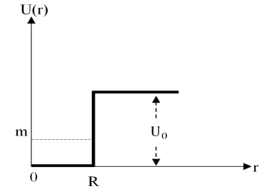
Figure 1: Potential landscape of a QD with radius $R$.

According to Figure 1, we distinguish between two regions in order to explicitly determine the solutions of the energy spectrum. Consequently, the general solutions to the radial equation (16), which are regular at the origin and decay exponentially as $r\rightarrow\infty$, are given in terms of $M\left(n_{\sigma},\left|\xi-\frac{\sigma}{2}\right|+1,\left|G\right|r^{2}\right)$ inside the QD and $U\left(n_{\sigma},\left|\xi-\frac{\sigma}{2}\right|+1,\left|G\right|r^{2}\right)$ outside the QD. These are

$${{\phi_{\sigma}^{\tau}}}(r)=2^{\left(1+\left|\xi-\sigma/2\right|\right)/2}e^{-\left|G\right|r^{2}/2}r^{\left(\left|\xi-\frac{\sigma}{2}\right|+1/2\right)}\left\{\begin{array}[]{cc}\alpha_{\sigma}U\left({n_{\sigma}^{>}},\left|\xi-\frac{\sigma}{2}\right|+1,\left|G\right|r^{2}\right),&r>R\\ \beta_{\sigma}M\left({n_{\sigma}^{<}},\left|\xi-\frac{\sigma}{2}\right|+1,\left|G\right|r^{2}\right),&r<R\end{array}\right.$$ (21)

where $\sigma=\pm 1$ the upper sign corresponding to the A sublattice and the lower sign to the B one. We introduced the label $<,>$ to separate between eignenergies of the two regions such that $\epsilon_{<}\equiv E$ and $\epsilon_{>}\equiv E-U_{0}$. Note that, the absolute value of $G$ is introduced in order to consider the case of positive and negative effective magnetic field. In addition, we note that the solution ${\phi_{\sigma}^{\tau}}(r)$ depend on the valley index $\tau$ through (13). Such that $\phi_{+}^{+}(r)$ and $\phi_{-}^{+}(r)$ are envelope wave functions of A and B sublattices for the valley $K$, and $\phi_{+}^{-}(r)$, $\phi_{-}^{-}(r)$ for the valley $K^{\prime}$.

At this stage, it is natural to ask about the eigenvalues associated to the bound states of our system. To answer this inquiry we use the matching conditions of the spinors at the interface $r=R$ to end up with the condition for the existence of bound states

$$\frac{\alpha_{+}}{\alpha_{-}}\ \frac{U\left(n_{+}^{>},|\xi-\frac{1}{2}|+1,|G|R^{2}\right)}{U\left(n_{-}^{>},|\xi+\frac{1}{2}|+1,|G|R^{2}\right)}=\frac{\beta_{+}}{\beta_{-}}\ \frac{M\left(n_{+}^{<},|\xi-\frac{1}{2}|+1,|G|R^{2}\right)}{M\left(n_{-}^{<},|\xi+\frac{1}{2}|+1,|G|R^{2}\right)}$$ (22)

where the ratios $\alpha_{+}/\alpha_{-}$ and $\beta_{+}/\beta_{-}$ can be explicitly determined by making use of the coupled first-order differential equation (15). The sign of $G$ depends on whether the oscillator frequency $\omega$ is larger or smaller than the cyclotron frequency $\omega_{c}$.

It is worthwhile investigating the basic features of of the above results and underlying their interesting properties. In this context, we would like to show how the valley degeneracy can be lifted by the presence of a constant magnetic field normal to the plane of the system together with a 2D Dirac-oscillator. This is of particular importance to form the valley filters, valves [30], or qubits [31] and spin qubits [32] in graphene. To this end, we consider three different cases corresponding to the relative strength of the magnetic field ($\omega_{c}$) with respect to the oscillator coupling ($\omega$).

3.2 Oscillating with same frequency

We study the first case were the oscillator frequency is tuned to resonate with the cyclotron frequency, i.e. $w\approx w_{c}$, which it is equivalent to consider $G=\lambda\Delta^{\prime}$ with $\Delta^{\prime}=\omega_{c}-\omega$. By requiring ${|\Delta^{\prime}|\ll\lambda}$ we show that the hypergeometric functions reduce to bessel functions [34]

$$U\left(n^{>},j,z\right)=\frac{2}{\Gamma\left(1-j+n^{>}\right)}(zn^{>})^{(1-j)/2}K_{j-1}\left(2\sqrt{zn^{>}}\right)$$ (23)

$$M\left(n^{<},j,z\right)=\Gamma(j)\left(-zn^{<}\right)^{(1-j)/2}J_{j-1}\left(2\sqrt{-zn^{<}}\right)$$ (24)

and the characteristic equation (22) takes the form according to $\xi>0$

$$\frac{\sqrt{\lambda^{2}-(E-U)^{2}}}{\sqrt{E^{2}-\lambda^{2}}}\frac{K_{\xi-\frac{1}{2}}\left(\sqrt{\lambda^{2}-(E-U)^{2}}R\right)}{K_{\xi+\frac{1}{2}}\left(\sqrt{\lambda^{2}-(E-U)^{2}}R\right)}=-\frac{E-U-\tau\lambda}{E-\tau\lambda}\frac{J_{\xi-\frac{1}{2}}\left(\sqrt{E^{2}-\lambda^{2}}R\right)}{J_{\xi+\frac{1}{2}}\left(\sqrt{E^{2}-\lambda^{2}}R\right)}$$ (25)

or $\xi<0$

$$\frac{\sqrt{\lambda^{2}-(E-U)^{2}}}{\sqrt{E^{2}-\lambda^{2}}}\frac{K_{-\xi-\frac{1}{2}}\left(\sqrt{\lambda^{2}-(E-U)^{2}}R\right)}{K_{-\xi+\frac{1}{2}}\left(\sqrt{\lambda^{2}-(E-U)^{2}}R\right)}=-\frac{E-U+\tau\lambda}{E+\tau\lambda}\frac{J_{-\xi-\frac{1}{2}}\left(\sqrt{E^{2}-\lambda^{2}}R\right)}{J_{-\xi+\frac{1}{2}}\left(\sqrt{E^{2}-\lambda^{2}}R\right)}.$$ (26)

We notice that there is a mapping between both of the two last equations, which is assured by the change $\xi\rightarrow-\xi$ and $\tau\rightarrow-\tau$. In general, these two equations can not be solved in the closed form.

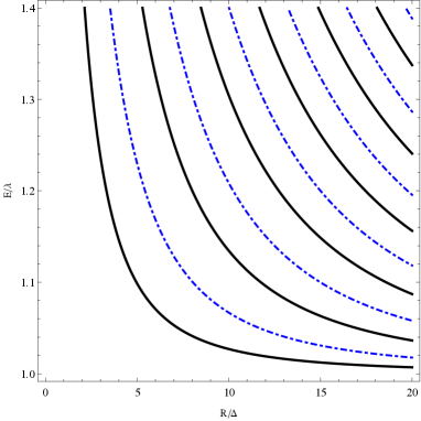
Figure 2: Energy levels of a circular quantum dot as a function of the dot radius $R$ for $\xi=\frac{1}{2}$ and $U=1.5\ \lambda$, with $\Delta=\hbar v_{F}/\lambda$. The energy levels corresponding to the $K$ and $K^{\prime}$ valleys are shown by the solid curve ($\tau=1$) and the blue dot dashed curve ($\tau=-1$) , respectively.

Results for the energy levels as a function of the dot radius are shown in Figure 2 for $\xi=\frac{1}{2}$ and $U=1.5\ \lambda$. The black solid and blue dot dashed curves correspond to the $K$ and $K^{\prime}$ valleys, respectively. Note that the case $\xi=-\frac{1}{2}$ for the same valley is also presented in both curves in Figure 2, which can be discussed by taking into account of the symmetry $E(\xi,\tau)=E(-\xi,-\tau)$ exhibited by our system. It may be noted that the solution for the two curves are different for the same valley. This can be explained by the fact that for the same valley we have $E(\xi)\neq E(-\xi)$. In fact, we can easily see from (25) and (26) that the energy verify $E(\xi,\tau)=E(-\xi,-\tau)$ and $E(\xi,\tau)\neq E(-\xi,\tau)$, which helps us to study the valley degeneracy by a Dirac oscillator. However, the results show that the valley degeneracy is not broken, in this case, if we include both sign of $\xi$. Our results are in agreement with previous calculations of bound-state energies for zero magnetic field [35]. In summary, it is clearly seen that when the oscillator frequency is tuned to resonate with the cyclotron frequency, the Dirac oscillator annihilates the effect of the magnetic field on our system and we find ourselves in the case of zero effective magnetic field. At zero effective magnetic field, the degeneracy of the levels in the two valleys is clearly displayed.

3.3 Strong magnetic field

Now, we study the case when the cyclotron frequency is much larger than the oscillator frequency, i.e. $w_{c}\gg w$, then $s=1$ and $G\approx\lambda\omega_{c}$. It may be noted that the effect of the oscillator interaction is to produce an effective magnetic field along the positive $z$-direction that produces the effective quantized Landau levels.

In this case we arrive, after applying the boundary conditions and finding both ratios, at the following characteristic equation for $\xi>0$

$$\frac{E-U+\tau\lambda}{4G}\ \frac{U(n_{1}^{>}+\xi+\frac{1}{2},\xi+\frac{1}{2},GR^{2})}{U(n_{1}^{>}+\xi+\frac{1}{2},\xi+\frac{3}{2},GR^{2})}=\frac{\xi+\frac{1}{2}}{E-\tau\lambda}\ \frac{M(n_{1}^{<}+\xi+\frac{1}{2},\xi+\frac{1}{2},GR^{2})}{M(n_{1}^{<}+\xi+\frac{1}{2},\xi+\frac{3}{2},GR^{2})}$$ (27)

and for $\xi<0$

$$\frac{1}{E-U+\tau\lambda}\ \frac{U(n_{1}^{>},-\xi+\frac{1}{2},GR^{2})}{U(n_{1}^{>}+1,-\xi+\frac{3}{2},GR^{2})}=\frac{\xi-\frac{1}{2}}{E+\tau\lambda}\ \frac{M(n_{1}^{<},-\xi+\frac{1}{2},GR^{2})}{M(n_{1}^{<}+1,-\xi+\frac{3}{2},GR^{2})}$$ (28)

where the used quantum number is given by

$$n_{1}^{<,>}=\frac{\lambda^{2}-\epsilon_{<,>}^{2}}{4|G|}.$$ (29)

Figure 3 shows the energies of the bound states in a graphene QD as function of the dot radius $R$ for small effective magnetic field. In this Figure, we show the low-lying bound states for $\xi=\pm\frac{1}{2},\ \pm\frac{3}{2}$ with $U=10\delta$/$U=20\delta$ (Figure 3 (a)/(b)) and $\lambda=10\delta$. We can clearly show that for zero effective magnetic field the degeneracy of the levels in the two valleys is not broken. This is in agreement with the results found in the first case when the oscillator frequency is tuned to resonate with the cyclotron frequency. However, by increasing the effective magnetic field, the valleys degeneracy is broken. This allows us to conclude that the oscillator interaction, which allow to produce an effective magnetic field, can be used to control the orbital degeneracy. In addition, we show that the number of the bound states depend on the electrostatic potential. In fact, by increasing $U$ the number of bound states decrease.

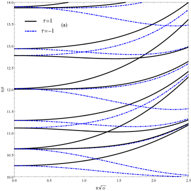
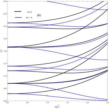
Figure 3: Energy levels of a circular quantum dot as a function of the dot radius $R$ with $\lambda=10\ \delta$, $U=10\ \delta$/ $U=20\ \delta$ ((a)/(b)) and we have introduced the quantum dot level spacing $\delta=\hbar v_{F}/R$. The energy levels corresponding to the $K$ and $K^{\prime}$ valleys are shown by the solid curve ($\tau=1$) and the dot dashed curve ($\tau=-1$), respectively. We show the low-lying bound states for $\xi=\pm\frac{1}{2},\ \pm\frac{3}{2}$.

In Figure 4 we show the energies of the bound states in a graphene QD as function of the dot radius $R$ for large effective magnetic field for $\xi=\pm\frac{1}{2},\ \pm\frac{3}{2},\ \pm\frac{5}{2}$. The solid and dot dashed curve correspond respectively to the $K$ and $K^{\prime}$ valleys. The results show that for large effective magnetic field the energy levels converge to the bulk Landau Levels. In addition, the states that are degenerate for zero effective magnetic field correspond to opposite values of the angular momentum $\xi$ in different valleys. We note that our results are in agreement with previous calculations of bound-state energies in presence of magnetic field applied perpendicular to the graphene plane [35].

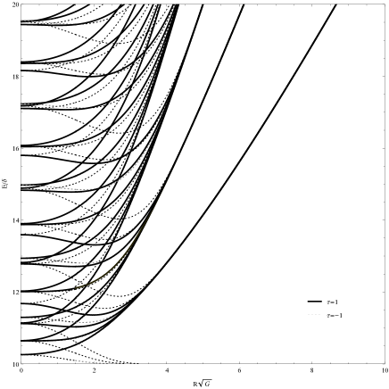
Figure 4: Energy levels of a circular quantum dot as a function of the dot radius $R$ with $m=10\ \delta$, $U=\lambda$ and we have introduced the quantum dot level spacing $\delta=\hbar v_{F}/R$. The energy levels corresponding to the $K$ and $K^{\prime}$ valleys are shown by the solid curve ($\tau=1$) and the dot dashed curve ($\tau=-1$) respectively. We show the bound states for large effective magnetic field with $\xi=\pm\frac{1}{2},\ \pm\frac{3}{2},\ \pm\frac{5}{2}$.

3.4 Weak magnetic field

In the third case we suppose that the cyclotron frequency is much smaller than the oscillator frequency, namely $\omega_{c}\ll\omega$, with $G\approx-\lambda\omega$, or $s=-1$. It may be noted that in this situation the effect of the oscillator interaction is to produce an effective magnetic field along the negative $z$-direction. In fact, this can be done by interchanging the confinement frequency $\omega$ with the cyclotron one $\omega_{c}$.

By using the above consideration, we obtain from (22) the characteristic equation for the allowed eigenenergies $E$ of the QD. Indeed, for $\xi>0$ we have

$$\frac{1}{E-U-\tau\lambda}\ \frac{U(n^{>}_{1},\xi+\frac{1}{2},-GR^{2})}{U(n^{>}_{1}+1,\xi+\frac{3}{2},-GR^{2})}=\frac{-\xi-\frac{1}{2}}{E-\tau\lambda}\ \frac{M(n^{<}_{1},\xi+\frac{1}{2},-GR^{2})}{M(n^{<}_{1}+1,\xi+\frac{3}{2},-GR^{2})}$$ (30)

and for $\xi<0$ reads as

$$\frac{E-U-\tau\lambda}{4G}\ \frac{U(n^{>}_{1}-\xi+\frac{1}{2},-\xi+\frac{1}{2},-GR^{2})}{U(n^{>}_{1}-\xi+\frac{1}{2},-\xi+\frac{3}{2},-GR^{2})}=\frac{\xi-\frac{1}{2}}{E+\tau\lambda}\ \frac{M(n^{<}_{1}-\xi+\frac{1}{2},-\xi+\frac{1}{2},-GR^{2})}{M(n^{<}_{1}-\xi+\frac{1}{2},-\xi+\frac{3}{2},-GR^{2})}.$$ (31)

It is important to note that (30) is obtained from (28) by the following mappings

$$\xi\longrightarrow-\xi,\qquad\tau\longrightarrow-\tau,\qquad G\longrightarrow-G$$ (32)

which can also be used to derive (31) from (27) in similar way as before. Moreover, the bound-state levels for negative effective magnetic field can be found by using the symmetry

$$E(\xi,\tau,G)=E(-\xi,-\tau,-G).$$ (33)

In both cases (positive and negative effective magnetic fields), the valley degeneracy is controllably broken by the presence of the effective magnetic field corresponding to our system.

4 Conclusion

We considered the Dirac equation in (2+1)-dimensions in the presence of a constant magnetic field together with a two-dimensional Dirac-oscillator potential coupling. Indeed, using a similarity transformation, we formulated our problem in terms of the polar coordinate representation that allows us to handle easily the exact relationship between spinor components. Then, we got the solutions to the energy spectrum of the Dirac equation for a gate-tunable graphene QD.

We discussed our results based on different physical parameters. In fact, we considered three cases, whether the cyclotron frequency is similar or larger/smaller compared to the oscillator frequency. This suggests defining an effective magnetic field that produces the effective quantized Landau levels. Our results were employed to discuss three important limiting cases those concern the weak, strong and fine tuned magnetic field situations.

We studied the effective magnetic field dependence of energy levels. Indeed, we showed that the degeneracy of the valley is controllably broken by the effective magnetic field. In the fine tuned magnetic field cases (zero effective magnetic field), we found that the degeneracy of the levels in the two valleys is clearly displayed. Then, we analyzed in detail the case when the cyclotron frequency is much larger than the oscillator frequency (strong magnetic field). It has also been shown that at zero effective magnetic field, the valley degeneracy are not broken. However, by increasing the effective field we showed that the valley degeneracy are broken.

In addition, when the magnetic field is turned off the problem becomes a pure Dirac oscillator, which leads to the creation of a negative effective magnetic field. These results showed that it is possible to control both spin and valley degeneracy by the effective magnetic field corresponding to our system. One can note that our results have an importance in forming valley filters as well as spin qubits in graphene quantum dots.

References

- [1] M. Grundmann, F. Heinrichsdorff, C. Ribbat, M.-H. Mao and D. Bimberg, Appl. Phys. B: Lasers Opt. 69, 413 (1999).
- [2] T. Pohjola, D. Boese, H. Schoeller, J. König and G. Sch n, Physica B 284, 1762 (2000).
- [3] J. L. West and N. J. Halas, Annu. Rev. Biomed. Eng. 5, 285 (2003).
- [4] D. Vanmaekelbergh and P. Liljeroth, Chem. Soc. Rev. 34, 299 (2005).
- [5] H. Arya, Z. Kaul, R. Wadhwa, K. Taira, T. Hirano and S. C. Kaul, Biochem. Biophys. Res. Commun. 329, 1173 (2005).
- [6] E. J. Gansen, M. A. Rowe, M. B. Greene, D. Rosenberg, T. E. Harvey, M. Y. Su, R. H. Hadfield, S. W. Nam and R. P. Mirin, Nat. Photonics 1, 585 (2007).
- [7] R. E. Prange and S. M. Girvin (Springer, New York) (1990).
- [8] K. S. Novoselov, A. K. Geim, S. V. Morozov, D. Jiang, Y. Zhang, S. V. Dubonos, I. V. Grigorieva and A. A. Firsov, Science 306, 666 (2004).
- [9] K. S. Novoselov, D. Jiang, T. Booth, V. V. Khotkevich, S. M. Morozov and A. K. Geim, Proc. Nat. Acad. Sci. 102, 10451 (2005).
- [10] A. K. Geim and K. S. Novoselov, Nat. Mater. 6, 183 (2007).
- [11] M. I. Katsnelson, K. S. Novoselov and A. K. Geim, Nat. Phys. 2, 620 (2006).
- [12] T. Chakraborty Quantum Dots (Amsterdam: Elsevier) (1999).
- [13] P. G. Silvestrov and K. B. Efetov, Phys. Rev. Lett. 98, 016802 (2007).
- [14] A. Matulis and F. M. Peeters, Phys. Rev. B 77, 115423 (2008).
- [15] M. Moshinsky and A. Szczepaniak, J. Phys. A 22, L817 (1989).
- [16] J. Bentez, R. P. Martnez y Romero, H. N. N ez-Y pez and A. L. Salas-Brito, Phys. Rev. Lett. 64, 1643 (1990).
- [17] P. Rozmej and R. Arvieu, J. Phys. A 32, 5367 (1999).
- [18] K. Nouicer, J. Phys. A. 39, 5125 (2006).
- [19] A. Bermudez, M. A. Martin-Delgado and A. Luis, Phys. Rev. A 77, 033832 (2008).
- [20] R. Gerritsma, G. Kirchmair, F. Zähringer, E. Solano, R. Blatt and C.F. Roos, Nature 463, 68 (2010).
- [21] D. Dutta, O. Panella and P. Roy, Ann. Phys. 331, 120 (2013).
- [22] S. Longhi, Opt. Lett. 35, 1302 (2010).
- [23] E. Sadurní, J. M. Torres and T. H. Seligman, J. Phys. A 43, 285204 (2010).
- [24] C. Quimbay and P. Strange, arXiv:1311.2021 (2013).
- [25] J. A. Franco-Villafañe, E. Sadurní, S. Barkhofen, U. Kuhl, F. Mortessagne and T. H. Seligman, Phys. Rev. Lett. 111, 170405 (2013).
- [26] A. Jellal, A. D. Alhaidari and H. Bahlouli, Phys. Rev. A 80, 012109 (2009).
- [27] H. Bahlouli, A. Jellal and Y. Zahidi, Int. J. Geo. Meth. Mod. Phys. 11, 1450036 (2014).
- [28] G. Giovannetti, P. A. Khomyakov, G. Brocks, P. J. Kelly and J. van den Brink, Phys. Rev. B 76, 073103 (2007).
- [29] S. Y. Zhou, G.-H. Gweon, A. V. Fedorov, P. N. First, W. A. de Heer, D.-H. Lee, F. Guinea, A. H. Castro Neto and A. Lanzara, Nat. Mater. 6, 770 (2007).
- [30] A. Rycerz, J. Tworzydlo and C. W. J. Beenakker, Nat. Phys. 3, 172 (2007).
- [31] P. Recher, B. Trauzettel, A. Rycerz, Y. M. Blanter, C. W. J. Beenakker and A. F. Morpurgo, Phys. Rev. B 76, 235404 (2007).
- [32] B. Trauzettel, D. Bulaev, D. Loss and G. Burkard, Nat. Phys. 3, 192 (2007).
- [33] M. Moshinsky, Y. Smirnov, The Harmonic Oscillator in Modern Physics, Contemporary Concepts in Physics, Harwood Academic Publishers, (1996).
- [34] M. Abramowitz and I. A. Stegun, (Dover, New York) (1965).
- [35] P. Recher, J. Nilsson, G. Burkard and B. Trauzettel, Phys. Rev. B 79, 085407 (2009).