Dissolution on Titan and on Earth: Towards the age of Titan’s karstic landscapes

• Thomas Cornet (tcornet@sciops.esa.int), European Space Agency (ESA), European Space Astronomy Centre (ESAC), P.O. BOX 78, 28691 Villanueva de la Canada (Madrid), Spain.

• Daniel Cordier, Université de Franche-Comté, Institut UTINAM, CNRS/INSU, UMR 6213, 25030 Besançon Cedex, France.

• Tangui Le Bahers, Université de Lyon, Université Claude Bernard Lyon 1, ENS Lyon, Laboratoire de Chimie UMR 5182, 46 allée d’Italie, F-69007 Lyon Cedex 07, France.

• Olivier Bourgeois, LPG Nantes, UMR 6112, CNRS, OSUNA, Université de Nantes, 2 rue de la Houssinière, BP92208, F-44322 Nantes Cedex 3, France.

• Cyril Fleurant, LETG - UMR CNRS 6554, Université d’Angers, UFR Sciences, 2 bd Lavoisier, F-49045 Angers Cedex 01, France.

• Stéphane Le Mouélic, LPG Nantes, UMR 6112, CNRS, OSUNA, Université de Nantes, 2 rue de la Houssinière, BP92208, F-44322 Nantes Cedex 3, France.

• Nicolas Altobelli, European Space Agency (ESA), European Space Astronomy Centre (ESAC), P.O. BOX 78, 28691 Villanueva de la Canada (Madrid), Spain.

Paper published in JGR Planets, April 2015, available at http://onlinelibrary.wiley.com/doi/10.1002/2014JE004738/full.

Abstract Titan’s polar surface is dotted with hundreds of lacustrine depressions. Based on the hypothesis that they are karstic in origin, we aim at determining the efficiency of surface dissolution as a landshaping process on Titan, in a comparative planetology perspective with the Earth as reference. Our approach is based on the calculation of solutional denudation rates and allow inference of formation timescales for topographic depressions developed by chemical erosion on both planetary bodies. The model depends on the solubility of solids in liquids, the density of solids and liquids, and the average annual net rainfall rates. We compute and compare the denudation rates of pure solid organics in liquid hydrocarbons and of minerals in liquid water over Titan and Earth timescales. We then investigate the denudation rates of a superficial organic layer in liquid methane over one Titan year. At this timescale, such a layer on Titan would behave like salts or carbonates on Earth depending on its composition, which means that dissolution processes would likely occur, but would be 30 times slower on Titan compared to the Earth due to the seasonality of precipitation. Assuming an average depth of 100 m for Titan’s lacustrine depressions, these could have developed in a few tens of millions of years at polar latitudes higher than 70^∘ N and S, and a few hundreds of million years at lower polar latitudes. The ages determined are consistent with the youth of the surface ($<1$ Gyr) and the repartition of dissolution-related landforms on Titan.

1 Introduction

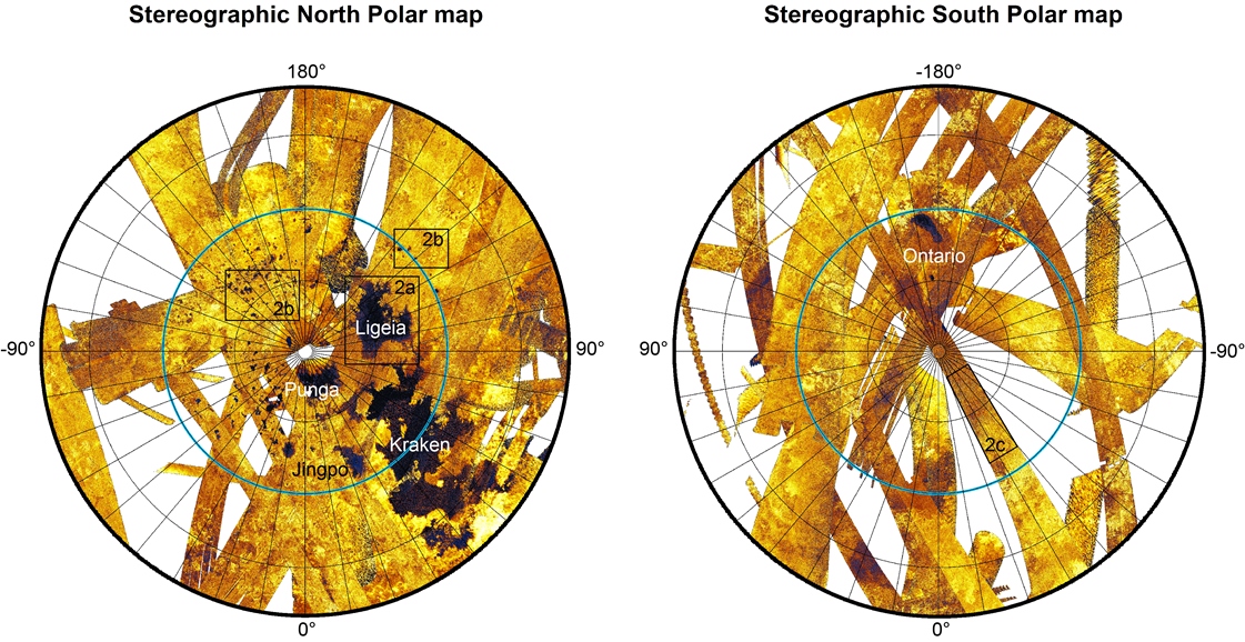
Figure 1: RADAR SAR mosaic of the TA (2004) to T95 (2013) flybys in north and south polar stereographic projections (down to 55^∘ latitudes). All current lakes observed to date are located above 70^∘ in latitude (blue circles).

Along with the Earth, Saturn’s icy moon Titan is the only planetary body of the entire Solar System that possesses lakes and seas (Lopes et al., 2007; Stofan et al., 2007; Hayes et al., 2008). Some of these lakes and seas are currently covered by liquids, while others are not (Hayes et al., 2008). Most are located in the polar regions (Hayes et al., 2008; Aharonson et al., 2009), although a few occurrences have been reported at lower latitudes (Moore and Howard, 2010; Vixie et al., 2012). The currently-filled lakes and seas are located poleward of 70^∘ of latitude in both hemispheres whereas most empty depressions are located at lower latitudes (Figure 1) (Hayes et al., 2008; Aharonson et al., 2009).

Altogether, empty depressions, lakes, seas and fluvial channels, argue for the presence of an active “hydrological” cycle on Titan similar to that of the Earth, with exchanges between the subsurface (ground liquids), the surface (lakes, seas, fluvial channels) and Titan’s methane-rich atmosphere, where convective clouds and sporadic intense rainstorms have been imaged by the Cassini spacecraft instruments (Turtle et al., 2011a). Methane, rather than water as on Earth, probably dominates the cycle on Titan (Lunine et al., 2008) and thus constitutes one of the main components of the surface liquid bodies observed in the polar regions (Glein and Shock, 2013; Tan et al., 2013). Ethane, the main photodissociation product of methane (Atreya, 2007), is also implied in Titan’s lakes chemistry, as predicted by several thermodynamical models (Lunine et al., 1983; Raulin, 1987; Dubouloz et al., 1989; Cordier et al., 2009; Tan et al., 2013; Cordier et al., 2013a; Glein and Shock, 2013), or as identified in Ontario Lacus thanks to the Cassini/VIMS instrument (Brown et al., 2008).

Titan’s lakes are located in topographic depressions carved into the ground by geological processes that are poorly understood to date. The origin of the liquid would be related to precipitation, surface runoff and underground circulation, leading to the accumulation of liquids in local topographic depressions.

In the present work, we aim to constrain the origin and the age of these depressions. Section 2 first provides a brief overview of their geology and a discussion of their possible origin based on their morphological characteristics and from considerations about Titan’s surface composition and climate. Based on this discussion, we propose a new quantitative model, whereby the depressions have formed by the dissolution of a surface geological layer over geological timescales, such as in karstic landscapes on Earth.

In terrestrial karstic landscapes, the maximum quantity of mineral that can be dissolved per year, namely the solutional denudation rate, can be computed using a simple thermodynamics-climatic model presented in Section 3. The denudation rate depends on the nature of the surface material (solubility and density of the minerals) and on the climate conditions (precipitation, evaporation, surface temperature). Using this simple model, it is possible to determine theoretical timescales for the formation of specific karstic landforms on Earth, which are compared to relative or absolute age determinations in Section 4.

We apply the same model to Titan’s surface in Section 5. Section 5.1 is dedicated to the comparative study of denudation rates of pure solid organics in pure liquid methane, ethane and propane, and of common soluble minerals (halite, gypsum, anhydrite, calcite and dolomite), cornerstones of karstic landscapes development on Earth, in liquid water over terrestrial timescales. Section 5.2 describes the computation of denudation rates of pure solids and of mixed organic surface layers in liquid methane over Titan timescales by using the methane precipitation rates extracted from the GCM of Schneider et al. (2012). Based on these denudation rates, we compute the timescales needed to develop the typical 100 m-deep topographic depressions observed in the polar regions of Titan (Section 6) and compare them to timescales estimated from other observations (e.g. crater counting, dune formation).

2 Geology of Titan’s lacustrine depressions

2.1 Geomorphological settings

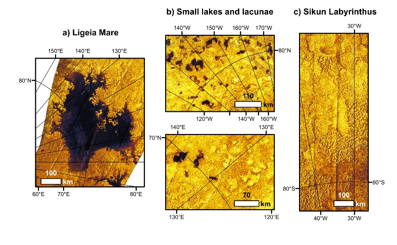
Figure 2: RADAR SAR views of Titan’s second largest sea Ligeia Mare (a), empty and liquid-covered lacustrine depressions (b), and the heavily dissected terrains of Sikun Labyrinthus (c). Ligeia Mare clearly differs in size and shape from the smaller lacustrine depressions, which suggests a different formation mechanism. Lacustrine depressions and labyrinthic terrains pertain to the class of features potentially related to the dissolution of the surface.

Seas and lacustrine depressions strongly differ in shape (Figure 2). On one hand, seas are large (several hundred km in width) and deep (from 150 to 300 - 400 m in depth) (Lorenz et al., 2008, 2014; Mastrogiuseppe et al., 2014). They possess dendritic contours and are connected to fluvial channels (e.g. Ligeia Mare, Figure 2a) (Stofan et al., 2007; Sotin et al., 2012; Wasiak et al., 2013). They seem to develop in areas associated with reliefs, which constitute some parts of their coastlines.

On the other hand, Titan’s lacustrine depressions (Figure 2b) develop in relatively flat areas. They lie between 300 and 800 meters above the level of the northern seas (Stiles et al., 2009; Kirk et al., 2012). They are typically rounded or lobate in shape and some of them seem to be interconnected (Bourgeois et al., 2008). Their widths vary from a few tens of km, such as for most of Titan’s lacunae, up to a few hundred km, such as Ontario Lacus or Jingpo Lacus. Their depths have been tentatively estimated to range from a few meters to 100 - 300 meters (Hayes et al., 2008; Kirk and Howington-Kraus, 2008; Stiles et al., 2009; Lorenz et al., 2013), with “steep”-sided walls (Mitchell et al., 2007; Bourgeois et al., 2008; Kirk and Howington-Kraus, 2008; Hayes et al., 2008). The liquid-covered depressions would lie 250 meters below the floor of the empty depressions (Kirk et al., 2007), which could be indicative of the presence of an alkanofer in the sub-surface, analog to terrestrial aquifers, filling or not the depressions depending on their base level (Hayes et al., 2008; Cornet et al., 2012). The depressions sometimes possess a raised rim, ranging from a few hundred meters up to 600 meters in height (Kirk et al., 2007; Kirk and Howington-Kraus, 2008). All these numbers are likely subject to modification following future improvements in depth-deriving techniques.

2.2 Geological origin of the depressions

The geological origin of the topographic depressions and how they are fed by liquids are still debated. The geometric analysis of the lakes by Sharma and Byrne (2010, 2011) led to the conclusion that, unlike on Earth, the formation mechanism of the lacustrine depressions cannot be derived from the analysis of their coastline shapes. Recently, Black et al. (2012) and Tewelde et al. (2013) showed that mechanical erosion due to fluvial activity would have a minor influence in landscape evolution on Titan. Given this context, several hypotheses are being explored to understand how Titan’s lakes have formed. These include:

1. cryovolcanic origin (Mitchell et al., 2007; Wood et al., 2007), forming topographic depressions in which lakes can exist, such as in terrestrial calderas (Acocella, 2007) or maars (Lorenz, 1986);

2. thermokarstic origin (Kargel et al., 2007; Mitchell et al., 2007; Harrisson, 2012), where the cyclic destabilization of a methane frozen ground would form topographic depressions, such as in periglacial areas on Earth where the permafrost cyclically freezes and thaws and forms thermokarst lakes, pingos or alases (French, 2007) ;

3. solutional origin (Mitchell et al., 2007; Bourgeois et al., 2008; Mitchell, 2008; Mitchell and Malaska, 2011; Malaska et al., 2011; Barnes et al., 2011; Cornet et al., 2012), where processes analogous to terrestrial karstic dissolution create topographic depressions, such as terrestrial sinkholes/dolines, playas and pans under various climates (Shaw and Thomas, 2000; Ford and Williams, 2007).

On one hand, the general lack of unequivocal cryovolcanic features on Titan tends to limit the likelihood of the cryovolcanic hypothesis (Moore and Pappalardo, 2011). A methane-based permafrost would be difficult to form on Titan due to the presence of nitrogen in the atmosphere (Lorenz and Lunine, 2002; Heintz and Bich, 2009). Its putative cyclic destabilization would also be challenging, given the tiny temperature variations between summer and winter, day and night, equator and poles (Jennings et al., 2009; Lora et al., 2011; Cottini et al., 2012) over all timescales (Aharonson et al., 2009; Lora et al., 2011). On the other hand, solid organics have been shown to be quite soluble in liquid hydrocabons under Titan’s surface conditions (Lunine et al., 1983; Raulin, 1987; Dubouloz et al., 1989; Cordier et al., 2009, 2013a, 2013b; Glein and Shock, 2013; Tan et al., 2013), provided that they are available at the surface. The observation of bright terrain around present lakes and inside of empty depressions, analogues of terrestrial evaporites produced by the evaporitic crystallization of dissolved solids, also strengthens this hypothesis (Barnes et al., 2011; MacKenzie et al., 2014).

On Earth, dissolution-related landforms are not restricted to sinkholes/dolines, pans or playa, which characterize relatively young karsts (Ford and Williams, 2007). Spectacular instances of reliefs nibbled by dissolution, known as cone/cockpit karsts, fluvio karsts or tower karsts, exist under temperate to tropical/equatorial climates, such as in China (Xuewen and Weihai, 2006; Waltham, 2008), Indonesia (Ford and Williams, 2007) or the Carribeans (Fleurant et al., 2008; Lyew-Ayee, 2010). The observation of possible mature karst-like terrains in Sikun Labyrinthus (Figure 2c) by Malaska et al. (2010), similar to these terrestrial karstic landforms also gives further credence to the hypothesis that lacustrine depressions on Titan are karstic in origin.

2.3 Composition of Titan’s solid surface

Titan’s surface can be divided into five main spectral units identified by the Cassini/VIMS instrument: bright terrain, dark equatorial dune fields or dark-brown units, blue units, 5 $\mu$m-bright units and the dark lakes (Barnes et al., 2007; Stephan et al., 2009). In the polar regions, the solid surface appears dominantly as bright terrain, lakes, and patches identified as the 5 $\mu$m-bright unit in VIMS data (Barnes et al., 2011; Sotin et al., 2012; MacKenzie et al., 2014). The spectral characteristics of the VIMS 5 $\mu$m-bright unit seen inside and around some polar (and equatorial) lacustrine depressions indicate the presence of various hydrocarbons and nitriles (Clark et al., 2010; Moriconi et al., 2010) and are not compatible with the presence of water ice (Barnes et al., 2009).

The origin of the organic materials is probably linked to the atmospheric photochemistry, which results in the formation of various hydrocarbons and nitriles (Lavvas et al., 2008a, b; Krasnopolsky, 2009) detected by Cassini (Cui et al., 2009; Magee et al., 2009; Clark et al., 2010; Coustenis et al., 2010; Vinatier et al., 2010; Cottini et al., 2012). Table 1 gives the estimated fluxes of some produced organics, as derived from several models. Most of these compounds could condense as solids and sediment onto the surface over geological timescales (Atreya, 2007; Malaska et al., 2011). Most of them would be relatively soluble in liquid alkanes (Raulin, 1987; Dubouloz et al., 1989; Cordier et al., 2009, 2013a; Glein and Shock, 2013; Tan et al., 2013).

It is therefore reasonable to assume that a superficial soluble layer, composed of organic products, exists at the surface of Titan. Episodic dissolution of this layer would be responsible for the development of karst-like depressions and labyrinthic terrains (Bourgeois et al., 2008; Malaska et al., 2010, 2011; Mitchell and Malaska, 2011; Cornet et al., 2012). Evaporitic crystallization could also occur after episodes of dissolution in the liquids, forming evaporite-like deposits (Barnes et al., 2011; Cornet et al., 2012; Cordier et al., 2013b; MacKenzie et al., 2014).

3 Solutional denudation rates on Earth

On Earth, karstic landforms develop thanks to the dissolution of carbonate (calcite, dolomite) and evaporite (gypsum, anhydrite, halite) minerals under the action of groundwater and rainfall percolating through pore space and fractures present in rocks. The mineral solubilities vary as a function of the environmental conditions (amount of rain and partial pressure of carbon dioxide) (Ford and Williams, 2007). Karstic landforms like dolines or sinkholes are often located under temperate to humid climates in carbonates (though gypsum or halite karsts also exist on Earth). They reach depths of up to a few hundred meters (Ford and Williams, 2007). Karsto-evaporitic landforms like pans are located under semi-arid to arid climates. They reach depths of up to a few tens of meters (Goudie and Wells, 1995; Bowen and Johnson, 2012). Evaporitic landforms like playas are located under arid climates. They are characterized by their extreme flatness and can occur in any kind of topographic depression (Shaw and Thomas, 2000).

Denudation rates (hereafter $DR$) in terrestrial karstic landscapes are primarily constrained by geological (age and physico-chemical nature of rocks) and climate (net precipitation rates evolution) analyses. For many limestone-dominated areas (the majority of karst areas), it is commonly assumed that dissolution features are mainly created in the epikarstic zone located in the top few meters below the surface (White, 1984; Ford and Williams, 2007). Classically, in karstic terrains, the chemical/solutional denudation rate $DR$ (in meters per Earth year, or m/Eyr) is related to the rock physico-chemical properties and the climate by the following equation (White, 1984; Tucker et al., 2001; Ford and Williams, 2007; Fleurant et al., 2008):

$$DR=\rho_{w}\,\frac{M_{\rm calcite}}{\rho_{\rm calcite}}\,\tau\,m_{\rm Ca},\qquad{\textrm{[m/Eyr]}}$$ (1)

where $\rho_{w}$ is the mass density of liquid water ($\simeq 1000$ kg/m³), $M_{\rm calcite}$ is the molar mass of calcite (in kg/mol), $\rho_{\rm calcite}$ is the mass density of calcite (in kg/m³), $\tau$ is the mean annual net precipitation rate (in m/yr), equivalent to the sum of runoff and infiltration or the difference between precipitation and evapotranspiration over long timescales (White, 2012), and $m_{\rm Ca}$ is the equilibrium molality of calcite (Ca²⁺ cations, in mol/kg), assuming an instantaneous dissolution. Following this equation, denudation rates depend linearly on the climate precipitation regime and on the molality of dissolved materials.

Molality calculations are provided in Appendix B for various soluble minerals, based on two thermodynamic hypotheses: an Ideal Solution Theory (IST, no preferential interactions between molecules) and an Electrolyte Solution Theory (EST, preferential interactions between molecules). We incorporated the effect of CO₂ gas dissolved in water, which acidifies water due to a series of intermediate reactions (one of which producing carbonic acid), and increases the dissolution rates of carbonates (calcite and dolomite, see Appendix B for more details). The partial pressure of CO₂ (hereafter $P_{CO_{2}}$, in atm) under different climates can be computed as follows (Ford and Williams, 2007):

$$\log P_{CO_{2}}=-3.47+2.09\,(1-e^{-0.00172\,AET}),$$ (2)

where $AET$ is the mean annual evapotranspiration rate in mm/Eyr. Applying the above formula gives $P_{CO_{2}}<3$ matm for arid areas, $3<P_{CO_{2}}<12$ matm for temperate areas and $P_{CO_{2}}>12$ matm for tropical or equatorial climates. The resulting typical values of denudation rates on Earth for common soluble minerals in liquid water are given in Table 2. Depending on the climatic conditions, denudation rates of salts are on the order of a few hundred $\mu$m to a few cm per Earth year, whereas denudation rates of carbonates are on the order of a few $\mu$m to a few hundred $\mu$m per Earth year. Note that chemical erosion is just one of the landshaping processes on Earth. Other mechanisms, such as mechanical erosion, would tend to increase the total denudation rate of a surface (Fleurant et al., 2008). The dissolved solids can take part in the crystallization of soluble deposits at the surface (e.g. calcretes or salt crusts in arid environments) or in the sub-surface (e.g. cements), when they saturate the liquids. They do not necessarily crystallize at the location where they dissolved (Ford and Williams, 2007).

4 Denudation rates to determine ages of terrestrial karstic landscapes

Using the denudation rates, theoretical timescales for the development of dissolution landforms of a given depth can be inferred. We test hereafter this hypothesis on terrestrial instances by comparing ages determined from the denudation rates and ages determined from relative or absolute chronology. For carbonates, the partial pressure of CO₂ is computed based on the MOD16 Global Evapotranspiration Product of the University of Montana/ESRI Mapping Center. The notation GEyrs, MEyrs and kEyrs will refer to timescales expressed respectively in Giga Earth years ($10^{9}$ years), Million Earth years ($10^{6}$ years) and kilo Earth years ($10^{3}$ years) in the following sections.

4.1 Example under a hyper-arid climate: the caves of the Mount Sedom diapir (Israel)

Mount Sedom is a $11\times 1.5$ km salt diapir located in Israel, 250 meters above the level of the Dead sea, under a hyper-arid climate (Frumkin, 1994, 1996). It is composed of a Pliocene-Pleistocene ($<7$ MEyrs) halite basis covered by a 5 - 50 m-thick layer composed of anhydrite and sandstones. Several sinkholes and caves exist in Mount Sedom (Frumkin, 1994).

In this part of Israel, the present-day hyper-arid climate leads to average rainfall rates of 50 mm/Eyr, of which 10 - 15 mm/Eyr constitutes the average effective rainfall rate ($\tau$). Gvishim and Mishquafaim Caves are respectively 60 m and 20 m-deep caves and are essentially carved into halite in the northern part of Mount Sedom. Radioisotopic age measurements in several caves of Mount Sedom give an Holocene age, about 8 kEyrs (and around 3.2 - 3.4 kEyrs from age measurements performed in Mishquafaim Cave) (Frumkin, 1996).

Assuming that underground dissolution is somewhat connected to the rainfall percolating through anhydrite and reaching halite, the denudation rates computed with our model (Equation 1) over this region are $DR\simeq 1.69-2.53$ mm/Eyr. The timescales required to form these caves would be between 23.7 and 35.5 kEyrs for Gvishim Cave, and between 7.9 and 11.8 kEyrs for Mishquafaim Cave, longer than those estimated from radioisotopic measurements.

However, it should be noted that Mount Sedom experiences a rather deep dissolution, the load of dissolved solids in the underground liquid water flowing in its caves being up to 3 times that of surface runoff (Frumkin, 1994). Therefore, considering that the denudation rate should be 3 times greater, we find timescales of development between 7.9 and 11.8 kEyrs for Gvishim Cave and between 2.6 and 3.9 kEyrs for Mishquafaim Cave, in better agreement with age measurements.

4.2 Example under a semi-arid climate: The Etosha super-pan (Namibia)

The Etosha Pan, located in Namibia under a semi-arid climate, is a flat 120$\times 60$ km karsto-evaporitic depression that has already been suggested as a potential analogue for Titan’s lacustrine depressions (Bourgeois et al., 2008; Cornet et al., 2012). The depression is about 15 to 20 m-deep at most, and has been carved into the carbonate layer essentially composed of calcretes and dolocretes lying ontop a middle Tertiary-Quaternary detritical sedimentary sequence that covers the Owambo basin (Buch and Rose, 1996; Hipondoka, 2005). This sedimentary sequence is believed to have accumulated under a semi-arid climate, relatively similar to the current one. The age of the calcrete layer is not known precisely, but its formation is believed to have started during the Miocene/Pliocene transition about 7 MEyrs ago (Buch, 1997; Buch and Trippner, 1997), or even later during the late Pliocene, 4 MEyrs ago (Miller et al., 2010). The Etosha Pan is believed to have developed at the expense of the calcrete layer since 2 MEyrs (Miller et al., 2010).

In the Owambo sedimentary basin, $AET\simeq 350$ mm/Eyr, yielding $P_{CO_{2}}=3$ matm. Precipitation rates during the summer rainy season reach up to 500 mm/Eyr, which leads to $\tau=150$ mm/Eyr at most. These conditions lead to $DR=6.5$ $\mu$m/Eyr in a substratum composed of calcite (calcrete) and $DR=5.6$ $\mu$m/Eyr in a substratum composed of dolomite (dolocrete). These denudation rates give an approximate age for the Etosha Pan of about 2.31 - 3.08 MEyrs in calcretes and 2.68 to 3.57 MEyrs in dolocretes. These ages are consistent with ages estimated from geological observations ($<4$ MEyrs).

4.3 Example under a temperate climate: the doline of Crveno Jezero (Croatia)

Crveno Jezero is a 350 m-wide collapse doline located in the Dinaric Karst of Croatia, under a presently mediterranean temperate climate. This part of the Dinaric Karst is essentially composed of limestones and dolomites that have been deposited during the Mesozoic (Triassic to Cretaceous), when the area was covered by shallow marine carbonate shelves (Vlahovic et al., 2002; Mihevc et al., 2010). The cliffs forming the doline are up to 250 m in height. The bottom of the depression is covered by a lake, named Red Lake, about 250 m-deep. The total depth of the doline is therefore about 500 m (Garasic, 2001, 2012).

Although the formation process of the collapse dolines in the area is still not completely understood, especially in terms of the relative importance and timing of the collapse compared to the dissolution in the development of the structure, the uplift linked to the formation of the Alps (Eocene-Oligocene) led to the exposure of these carbonates and their subsequent karstification since at least Oligo-Miocene times (last 30 MEyrs) (Sket, 2012). At some point, dissolution occurred to form an underground cave; then the load of the capping rocks exceeded their cohesion, leading to the brutal or progressive collapse of the cap in the empty space beneath. The timescale calculated for the doline formation therefore constitutes a higher estimate. Age determinations in the northern Dinaric caves have been performed and show that karstification would be older than 4 to 5 MEyrs (Zupan Hajna, 2012). Crveno Jezero thus developed between 4 and 30 MEyrs ago.

In this region of Croatia, $AET\simeq 500$ mm/Eyr, which leads to $P_{CO_{2}}=5.44$ matm. Annual mean precipitation rates are about 1100 mm/Eyr (Mihevc et al., 2010), leading to $\tau=600$ mm/Eyr. These parameters give $DR=31.8$ $\mu$m/Eyr in limestones dominated by calcite ($DR=27.5$ $\mu$m/Eyr in limestones dominated by dolomite). The time required to dissolve 500 m of calcite under these present conditions would be around 15.7 MEyrs (18.2 MEyrs in dolomite). It is likely that cap rocks fell into the cave, leading to a younger age (1 m of calcite and dolomite dissolve in about 31 and 36 kEyrs respectively). However, the age determined by our method is still consistent with the geological records.

4.4 Example under a tropical climate: the Xiaozhai tiankeng (China)

The Xiaozhai tiankeng is a 600 m-wide collapse doline located in the Chongqing province of China, under a tropical climate. The depth of this doline is evaluated between 511 and 662 m depending on the location (Xuewen and Weihai, 2006; Ford and Williams, 2007). It is organized into two major collapse structures, an upper 320 m-deep structure and a lower 342 m-deep shaft. The tiankeng developed into Triassic limestones in a karst drainage basin. It results from various surface and subsurface processes such as dissolution, fluid flows and collapse. Tiankengs of China would have formed during the late Pleistocene (last 128,000 Eyrs) (Xuewen and Weihai, 2006) under an equatorial monsoonal climate similar to nowadays, emplaced 14 MEyrs ago (Wang and Li, 2009).

In the area, annual precipitation rates are about 1500 mm/Eyr, for an annual evapotranspiration rate of about 800 mm/Eyr, which leads to $P_{CO_{2}}=0.0123$ atm and $\tau=700$ mm/Eyr. Under these conditions, $DR=49.6$ $\mu$m/Eyr (calcite) or $DR=42.6$ $\mu$m/Eyr (dolomite) and the timescale to form the Xiaozhai tiankeng would be between 10.3 and 13.3 MEyrs (calcite) and 12.0 and 15.5 MEyrs (dolomite), considerably longer timescales than those estimated from geological records. However, such a difference is to be expected, since the formation of gigantic tiankengs are subject to complex interconnected surface processes not taken into account in these simple calculations (collapse and underground circulation of water). This illustrates the limits of our method, generally over-estimating the ages of karstic features when they do not result from dissolution only.

5 Denudation rates on Titan

Equation 1 has to be adapted for Titan. From thermodynamics, we compute molar volumes ($V_{\rm m,i}$ in m³/mol, see Appendix C) and mole fractions at saturation ($X_{i,\rm sat}$, see Appendix B) instead of mass densities and molalities. We considered the Ideal and the non-ideal Regular Solutions Theories (IST and RST respectively) and ensured that our results are consistent with experimentally determined solubilities. The RST has been developed to determine the solubility of non-polar to slightly polar molecules, such as simple hydrocarbons or carbon dioxide, in non-polar solvents. It is less likely to be appropriate for polar molecules such as nitriles/tholins and water ice. We therefore always provide a comparison between the IST and the RST in order to assess the uncertainty of the calculation by using the RST for polar molecules (see also Appendix B). However, we consider the RST, which provides our lowest and more realistic solubilities (at least for hydrocarbons), as the most suited model for the study. We assume that dissolution is instantaneous, which is not unreasonable given the rapid saturation of solid hydrocarbons in liquid ethane inferred from recent dissolution experiments (Malaska and Hodyss, 2014), compared to the long geological timescales considered in our work. For a binary solute-solvent system, Equation 1 becomes:

$$DR_{i}=\frac{X_{i,\rm sat}}{1-X_{i,\rm sat}}\,\tau\,\frac{V_{{\rm m},i}^{S}}{V_{\rm m,solv}^{L}},\qquad\textrm{[m/Eyr]}$$ (3)

where $V_{{\rm m},i}^{S}$ and $V_{\rm m,solv}^{L}$ are the molar volumes of the solid (crystallized) phase and of the liquid phase respectively.

5.1 Comparison between Titan and the Earth over terrestrial timescales

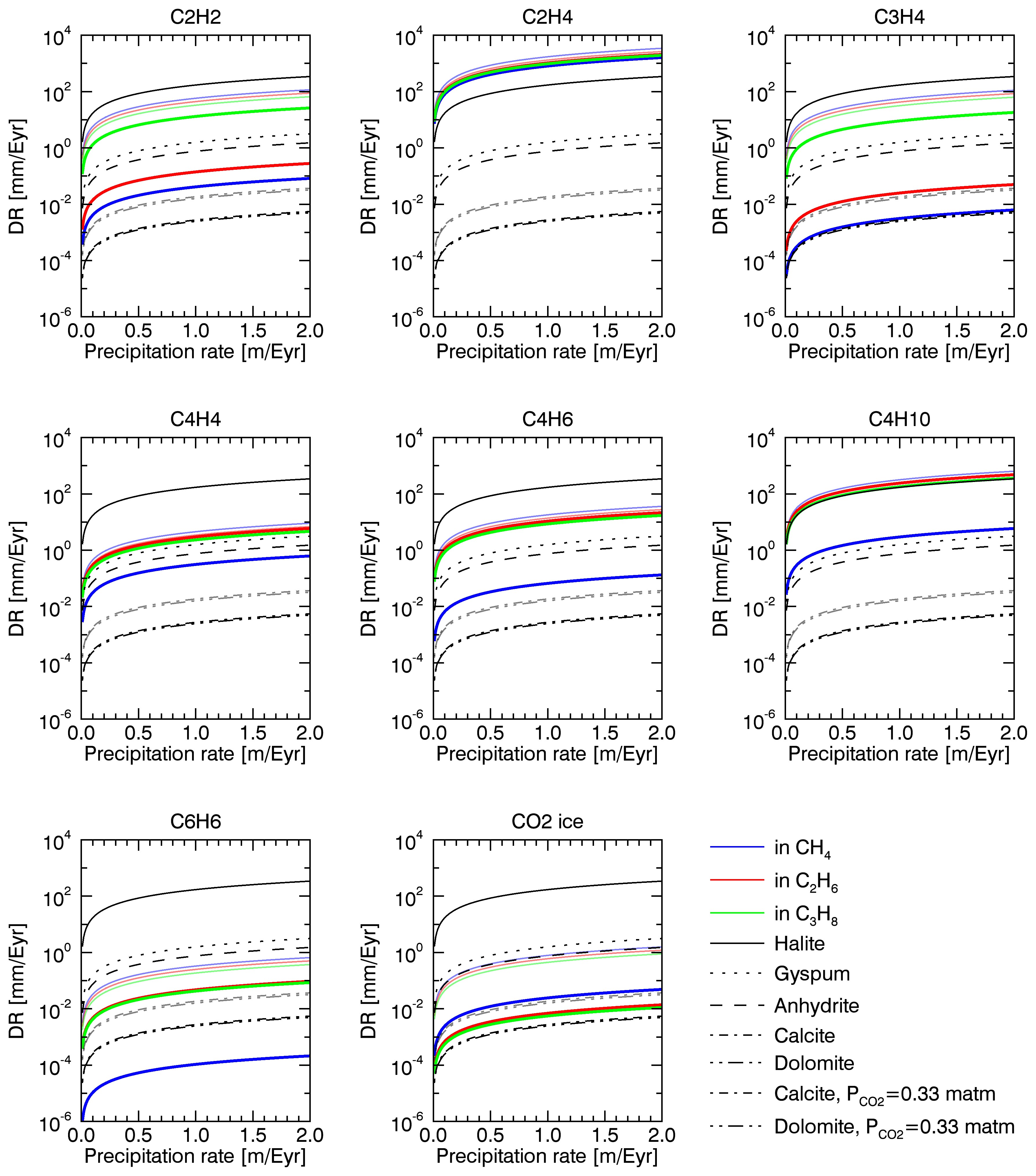
Figure 3: Denudation rates (in mm/Eyr) of non to slightly polar molecules (hydrocarbons and carbon dioxide ice) in Titan’s liquids at 91.5 K (light curves: IST, bold curves: RST) compared to those of Earth’s minerals in liquid water at 298.15 K (EST). The partial pressure of carbon dioxide for acid dissolution is set to 0.33 matm.

In order to compare the behavior of Titan’s solids in Titan’s liquids with that of minerals in liquid water on Earth, we computed Titan’s and Earth’s denudation rates over Earth timescales by varying the precipitation rate between 0 and 2 m/Eyr. This range of precipitation rates encompasses the expected range on Titan (up to 1.2 - 1.3 m/Eyr during the rainy season (Schneider et al., 2012)). It also covers the precipitation range between arid and tropical climates on Earth. This comparison is illustrated in Figures 3 (for hydrocarbons and carbon dioxide ice) and 4 (for nitriles and water ice), for which we fixed Titan’s temperature to 91.5 K (the surface temperature during the rainy season according to Schneider et al. (2012)) and Earth’s temperature to 298.15 K (with a partial pressure of carbon dioxide equal to 0.33 matm).

All organic compounds except C₁₁H₁₁N would behave like common mineral salts (halite, gypsum or anhydrite) according to the IST, which means that they would experience dissolution rates in the range of hundred $\mu$m to a few cm over one Eyr. According to the RST and assuming that the liquid is methane, C₂H₄ would behave like halite (cm-scale dissolution), C₄H₁₀ and C₄H₄ like gypsum (hundred $\mu$m to mm-scale dissolution), C₂H₂, C₃H₄, C₄H₆ and CO₂ like carbonates (up to hundred $\mu$m-scale dissolution). C₆H₆ and nitriles would be less soluble in methane than calcite is in pure liquid water, with the least soluble nitriles being C₁₁H₁₁N, HCN and CH₃CN. As expected, water ice is completely insoluble according to the RST, developed for non-polar molecules.

The denudation rates of all organic compounds are higher in ethane and propane than in methane. Nitriles and C₆H₆, which are poorly soluble in methane, are quite soluble in ethane and propane (except C₁₁H₁₁N, HCN and CH₃CN still under the calcite level) and reach denudation rates similar to those of carbonates or even gypsum. C₂H₂ and C₃H₄ would behave like carbonates (in ethane) or gypsum (in propane). C₄H₄ and C₄H₆ behave like salts in those liquids and are even more soluble than gypsum. C₄H₁₀ and C₂H₄ are halite-like materials, extremely soluble in ethane and propane. Therefore, the likelihood of developing dissolution landforms in a hydrocarbon dominated substrate, by analogy with the Earth, is high.

5.2 Present denudation rates on Titan over a Titan year

5.2.1 Net precipitation rates on Titan

Computing denudation rates over Titan timescales requires us to define the evolution of the net precipitation over one Titan year (1 Tyr $\simeq 29.5$ Earth years). Titan’s climate is primarily defined by a rainy warm “summer” season and a cold dry “winter” season, both spanning about 10 Earth years. Southern summers are shorter and more intense than those in the north (Aharonson et al., 2009). Precipitation occurs as sporadic and intense rainstorms during summer, when cloud formation is observed (Roe et al., 2002; Schaller et al., 2006, 2009; Rodriguez et al., 2009, 2011; Turtle et al., 2011a, b).

A few Global Circulation Models (GCM) attempt to describe, at least qualitatively, the methane cycle on Titan (e.g. Rannou et al. (2006), Mitchell (2008), Tokano (2009) and Schneider et al. (2012)). Usually, net accumulation of rain is predicted at high latitudes $>60^{\circ}$ during summer, in agreement with the presence of lakes, whereas mid-to-low latitudes experience net evaporation, in agreement with the absence of lakes and the presence of deserts. Quantitatively, the model predictions are subject to debate since they depend on their physics (e.g. cloud microphysics, size of the methane reservoir, radiative transfer scheme). Still, they remain our best estimates about Titan’s climate.

During the summer season, the model of Rannou et al. (2006) predicts net precipitation rates of methane lower than 1 cm/Eyr at 70^∘ latitude and up to 1 m/Eyr poleward of 70^∘, equivalent of a few $\mu$m to 2.7 mm/Earth day (Eday) respectively. The model of Mitchell (2008) predicts precipitation rates of about 2 mm/Earth day (Eday) in the polar regions and along an “Inter-Tropical Convergence Zone” (ITCZ), nearly moving “pole-to-pole”. The intermediate and moist models of Mitchell et al. (2009) predict precipitation roughly varying between 2 and 4 mm/Eday at the poles and along the ITCZ. These rates are consistent with those estimated in Mitchell et al. (2011) in order to reproduce the tropical storms seen in 2010 (Turtle et al., 2011a) and with those estimated by the model of Schneider et al. (2012). The model of Tokano (2009) also predicts similar precipitation rates (800 to 1600 kg/m² in half a Titan year, equivalent to precipitations between 3 and 6 mm/Eday).

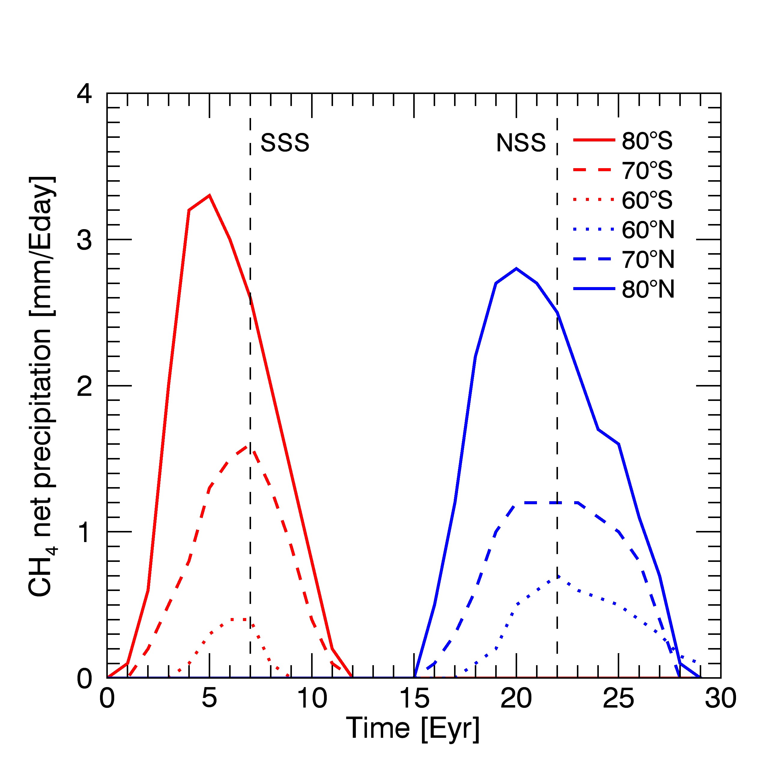
Figure 5: Net precipitation rates in mm/Earth day (Eday) at high southern and northern latitudes from Schneider et al. (2012) over a Titan year (29.5 Eyrs). SSS and NSS: Southern and Northern Summer Solstices.

Here, we use the methane net precipitation rates extracted from the GCM of Schneider et al. (2012) to compute the present-day denudation rate on Titan. Figure 5 represents the mean net precipitation rates at various polar latitudes. High latitudes $>80^{\circ}$ would be quite humid ($\tau=7-8$ m/Tyr). Lower latitudes would be less humid ($\tau=3-3.6$ m/Tyr at $70^{\circ}$, decreasing to $\tau=0.4-1.6$ m/Tyr at $60^{\circ}$). Southern low latitudes would be much drier than northern latitudes over a Titan year as a result of sparser but more intense rainstorms.

5.2.2 Case of pure compounds

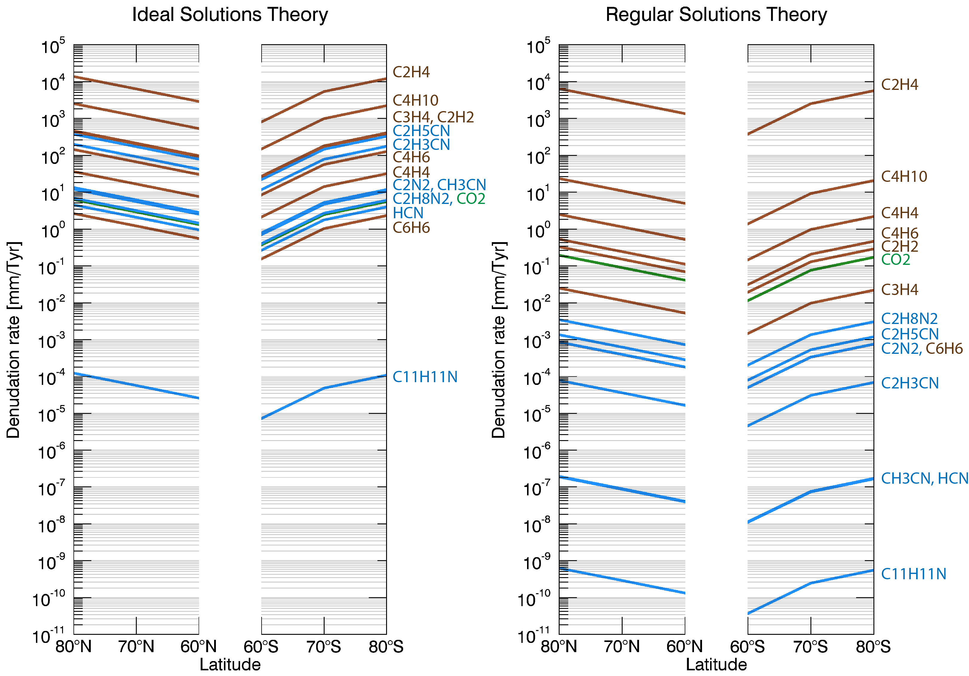
Figure 6: Denudation rates (in mm/Tyr) of Titan’s surface solids in liquid methane according to the methane net precipitation rates of Schneider et al. (2012) over an entire Titan year for the IST and RST approaches. In brown are represented simple hydrocarbons, in blue the nitriles and in green carbon dioxide.

Figure 6 illustrates the denudation rates of a surface composed of pure organic compounds exposed to methane rains at several southern and northern polar latitudes according to the IST and RST hypotheses. Ethane and propane are not shown since the model of Schneider et al. (2012) only considers methane, but the behavior of Titan’s solids in these liquids is already discussed in Section 5.1.

Over one Titan year, the denudation rates are the highest at high latitudes and the lowest at low southern latitudes. According to the IST, all compounds would experience dissolution on the order of a few mm to a few meters at almost all latitudes (salt-like material), except C₁₁H₁₁N, the denudation rate of which would be a few hundred nm. The dissolution of C₂H₈N₂, CO₂, HCN and C₆H₆ at 60^∘S however would be on the order of several hundred $\mu$m (carbonate-like material).

According to the RST, C₂H₄ and C₄H₁₀ denudation rates are between a few mm up to a few meters per Titan year (salt-like materials). The dissolution of C₄H₄, C₄H₆, C₂H₂, CO₂, C₃H₄ is $\mu$m to hundred $\mu$m-scale over a Titan year (carbonate-like materials). The denudation rates of nitriles and C₆H₆ are between $10^{-7}-10^{-10}$ mm/Tyr (for HCN, CH₃CN, C₁₁H₁₁N) and a few $\mu$m/Tyr (carbonate to siliceous-like materials).

At high latitudes $>70^{\circ}$, we do not see much differences between the northern and the southern denudation rates, as expected from the similarities in precipitation rate between the two poles shown in Figure 5. At low southern latitudes, net precipitation rates are too low over one Titan year to allow a rapid and significant dissolution. Interestingly, Ontario Lacus and Sikun Labyrinthus, two landforms compared with terrestrial karsto-evaporitic and karstic landforms (Malaska et al., 2010; Cornet et al., 2012), are observed at latitudes greater than 70^∘S, and no other well-developed dissolution-related landforms are seen at lower southern latitudes.

Therefore, if Titan’s surface is composed of pure hydrocarbons, dissolution processes are likely to occur but the formation of a karstic-like landscapes would be roughly 30 times slower on Titan than on Earth due to Titan’s seasonality in precipitation. Of course, this latter consideration depends on the actual composition of the surface, which is unlikely to be pure, and of the accuracy of the climate model used.

5.2.3 Case of a mixed surface layer

We now assume the presence of a surface layer, the composition of which is proportional to the accumulation rates at the surface ($h_{i}$) of solids coming from the atmosphere, calculated in the same way as Malaska et al. (2011) did:

$$h_{i}=p_{i}\,V^{S}_{\rm m,i}/N_{A},\qquad\textrm{[m/Eyr]}$$ (4)

where $p_{i}$ is the production rate of molecules (in molecules/m²/Eyr) listed in Table 1, $V^{S}_{\rm m,i}$ is the molar volume of the solid (or subcooled liquid if the former is not known, in m³/mol) and $N_{A}$ is the Avogadro number ($\simeq 6.022\times 10^{23}$ mol^-1). The composition of the mixed organic layer is then determined as percentages ($f_{i}$) of each organic compound in the layer (so that $f_{i}=h_{i}/\sum_{i}h_{i}$). This method allows us to consider the volume occupied by each molecule, which is important especially for tholins because these contribute up to 20 % on average to the total production rates of molecules, but they build up to $\simeq 50$ % of the total thickness of the surface deposits due to their higher molar volumes compared to those of simple hydrocarbons or nitriles.

We consider 3 cases for the surface composition: without tholins and with C₂H₈N₂ or C₁₁H₁₁N as tholins. Tholins production rate is that mentioned in Cabane et al. (1992). Methane precipitation rates are those of Schneider et al. (2012). The denudation rates for these mixed organic layers ($DR_{mix}$) are computed in a linear mixing model scheme where:

$$DR_{mix}=\sum_{i}f_{i}\,DR_{i}.\qquad\textrm{[m/Eyr]}$$ (5)

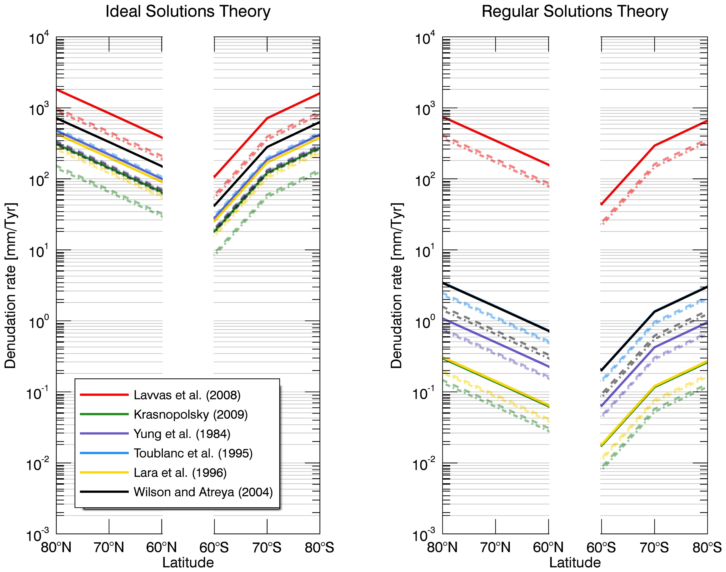
Figure 7: Denudation rates (in mm/Tyr) of Titan’s surface solids in liquid methane according to the Schneider et al. (2012) model net precipitation rates over an entire Titan year at various latitudes and for different surface layer compositions established from photochemical models, including (dashed lines) or not (solid lines) the influence of tholins (dashed line: with C₂N₈N₂ ; dashed-dot line: with C₁₁H₁₁N).

Figure 7 gives the repartition of denudation as a function of latitude and photochemical models at the end of a Titan year. According to the IST, the denudation rate of all mixed layers would be on the order of a few cm to a few meters over a Titan year (salt-like layers). According to the RST, the organic layer originating from the Lavvas et al. (2008b) model would be the most soluble (dissolution rates of a few cm to a few dm per Titan year, salt-like layer). The organic layers originating from the other models would be more carbonate-like layers over a Titan year (dissolution rates of a few tens of $\mu$m to a few mm per Titan year), whether tholins are included or not. The lowest solubility of all mixed layers is reached using a Krasnopolsky (2009)-type composition. Over a Titan year, the likelihood of developing dissolution-related landforms is therefore non-negligible, even if the surface is not composed of pure soluble simple solids. These mixed organic layers would behave like carbonate or salty terrestrial layers over a Titan year.

6 Discussion: How old are Titan’s karstic landscapes?

Despite the strong assumptions of the method described in Section 4 to infer timescales of formation of terrestrial karstic landforms (we consider only chemical erosion at equilibrium without significant climate changes over the past few MEyrs), the resulting ages are consistent with ages determined by relative or absolute chronology or constitute upper limits. Therefore, the determination of the age of the lacustrine depressions on Titan probably result in maximum timescales of development. Titan’s climate is believed to have remained quite stable over the recent past, with a small periodic insolation variation of $\pm 2$ W/m² at the poles during the last MEyr, for the current low insolation at the North pole (Aharonson et al., 2009). This probably brings some stability to the calculations.

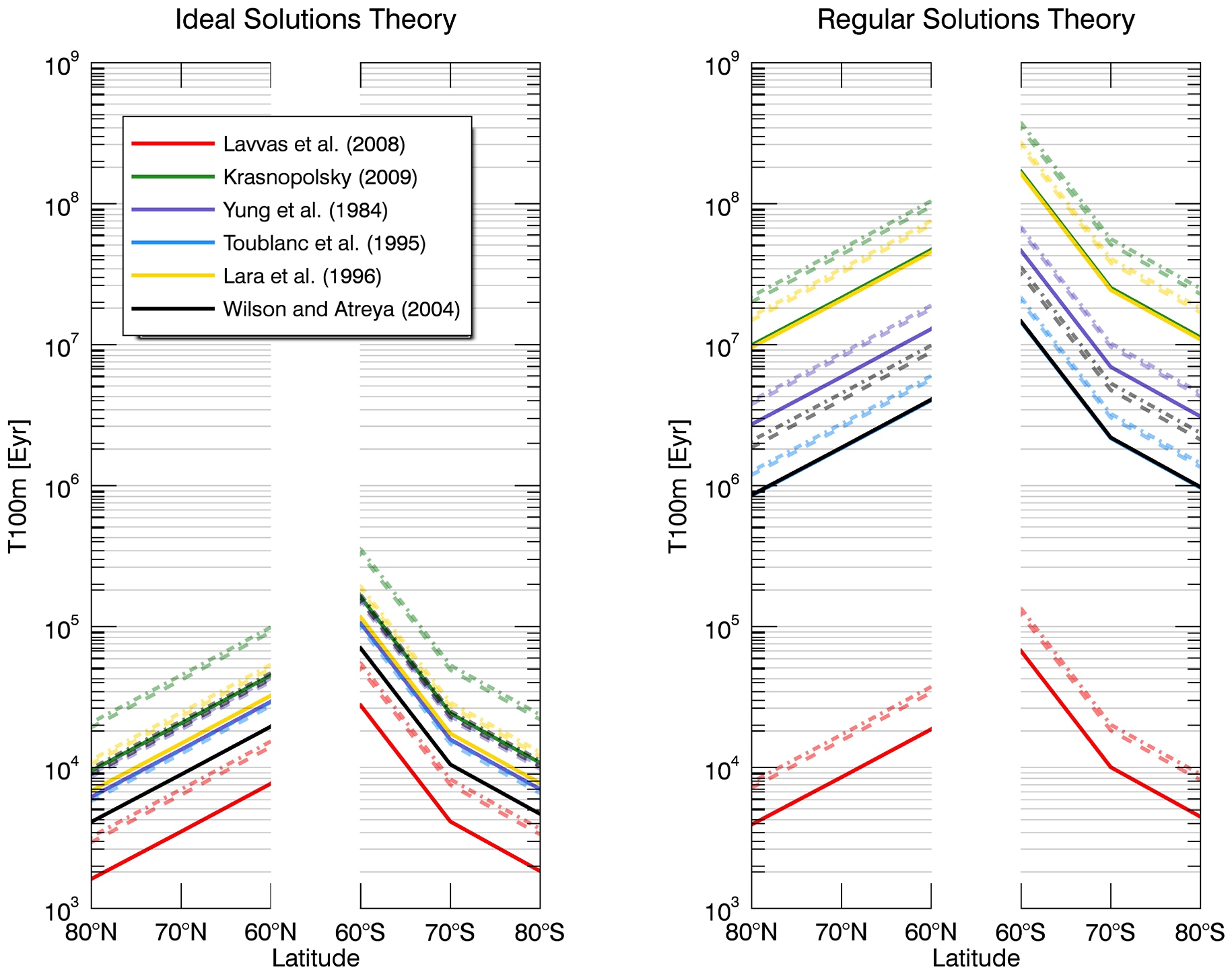
Figure 8: Same as Figure 7 but for the timescales of formation (in Eyr) of 100 m-deep depressions on Titan.

By applying our simple model, we compute the timescales needed to form a 100 m-deep depression by dissolution of a superficial mixed organic layer under the current climate conditions evaluated by Schneider et al. (2012). These are shown in Table 3 and Figure 8. We compute our formation timescales using both the IST and the RST since the solubility of polar molecules is not well constrained by the RST and could get closer to that computed using the IST. However, we consider timescales evaluated using the RST as our references since they present the most conservative values for the age of the lacustrine depressions.

Independent of the thermodynamic theory considered, Titan’s lacustrine depressions would be young. Among all the compositions tested, the time needed to carve a 100 m-deep depression by dissolution under current climate conditions at latitudes poleward of 70^∘ would be between a few kEyrs (IST) and 56 MEyrs (RST). At 60^∘N, a 100 m-deep depression would be created in 7.7 kEyrs (IST) to 104.6 MEyrs (RST) while the same depression would be created in 27.6 kEyrs (IST) to 375.1 MEyrs (RST) at 60^∘S. This strong difference between the two hemispheres could explain why Titan’s south polar regions are deprived of well developed lacustrine depressions compared to the North.

It should be noted that the hypothesized timescale difference between the northern and the southern low latitudes results from an extrapolation of Titan’s current climate to the past. Aharonson et al. (2009) showed that Croll-Milankovich-like cycle with periods of 45 (and 270) kEyrs could exist on Titan, resulting in a N-S reversal in insolation and likely subsequent climate conditions. Over geological timescales, the N-S differences in denudation rates and timescales estimated at these latitudes could be smoothed by these cycles. However, as noted earlier, we made the same extrapolation for the Earth, whose climate dramatically changed over time, without obtaining unreasonable formation timescales.

In any case, all these timescales are consistent with the youth of Titan’s surface as determined from:

1. crater counting ($0.3-1.2$ GEyrs, Neish and Lorenz (2012)),

2. dune sediment inventory ($50-730$ MEyrs, Sotin et al. (2012) and Rodriguez et al. (2014)),

3. the flattening of the poles due to the substitution of methane by ethane in clathrates (500 MEyrs if restricted to the poles or $0.3-1.7$ GEyrs if not, Choukroun and Sotin (2012))

4. the possible methane outgassing event ($1.7-2.7$ GEyrs, Tobie et al. (2006)).

In summary, the morphology of Titan’s lacustrine depressions suggests that dissolution occurs on Titan. The denudation rates of pure organic compounds and a mixed organic layer as compared to those of soluble minerals on Earth also supports this hypothesis. The timescales needed to dissolve various amounts of material as compared to the timescales of development of karstic landforms on Earth are also quite consistent in the sense that karstic landscapes are usually relatively young landscapes. Finally, the latitudinal repartition of denudation rates and timescales of dissolution is consistent with the latitudinal repartition of the possible dissolution-related landforms at the surface of Titan. The surface dissolution scenario for the origin of Titan’s lakes appears very likely and Titan’s lakes could be among the youngest features of the moon.

7 Conclusion

Titan’s lakes result from the filling of topographic depressions by surface or subsurface liquids. Their morphology led to analogies with terrestrial landforms of various origins (volcanic, thermokarstic, karstic, evaporitic or karsto-evaporitic). The karstic/karsto-evaporitic dissolution scenario seems to be the most relevant, given the nature of surface materials on Titan and its climate. We constrained the timescales needed for the formation of Titan’s depressions by dissolution, on the basis of the current knowledge on the development of terrestrial karsts.

We computed solutional denudation rates from the theory developed by White (1984). This simple theory needs three parameters: the solubilities and the densities of solids and liquids at a given temperature and a climatic parameter linked to the net precipitation rates onto the surface. We computed the solubilities of terrestrial minerals in liquid water at 25^∘C and tested the model by computing the denudation rates and timescales of formation of several terrestrial examples of karstic landforms.

We then applied the same model to Titan. We computed the solubilities of Titan’s surface organic compounds in pure liquid methane, ethane and propane at 91.5 K using different thermodynamic theories. We evaluated the molar volumes of liquid and solid Titan’s surface compounds at 91.5 K and we used the results of the recent GCM of Schneider et al. (2012) as input for the precipitation rates of methane on Titan, which allowed us to compute denudation rates at several latitudes. Denudation rates have then been computed for pure organic compounds at Earth and Titan timescales and have been compared to those determined for soluble minerals on Earth. We also computed denudation rates for three different compositions of the surface organic layer. Over one Titan year, these mixed layers of organic compounds behave like terrestrial salts or carbonates, which indicates their high susceptibility to dissolution, though these processes would be 30 times slower on Titan than on Earth due to the seasonality (rainfall occurs only during Titan’s summer).

We computed theoretical timescales for the formation of 100 m-deep depressions in mixed organic layers under present climatic conditions. As with dissolution landforms on Earth, Titan’s depressions would be young. At high polar latitudes, we found that the timescales of development for depressions are relatively short (on the order of 50 MEyrs at maximum to carve 100 m) and consistent with the young age of Titan’s surface. These timescales are consistent with the existence of numerous lacustrine depressions and dissected landscapes at these latitudes. At southern low latitudes, the computed timescales are as long as 375 MEyrs due to the low precipitation rates. This low propensity to develop depressions by dissolution is consistent with their relative absence/bare formation at low latitudes. Over geological timescales greater than those of Titan’s Croll-Milankovitch cycles (45 and 270 kEyrs), this difference would probably be strongly attenuated. However, climate model predictions are not presently available over geologic timescales, and the present-day seasonal climate variations are the best that can be currently constrained.

The results of these simple calculations are consistent with the hypothesis that Titan’s depressions most likely originate from surface dissolution. Theoretical timescales for the formation of these landforms are consistent with the other age estimates of Titan’s surface. Future works could include the effects of rain in equilibrium with the nitrogen, ethane and propane atmospheric gases in the raindrop composition (e.g. Graves et al. (2008) or Glein and Shock (2013)). Experimental constraints on the solubility of gases and solids in liquids thanks to recent technical developments for Titan experiments (Luspay-Kuti et al., 2012, 2014; Malaska and Hodyss, 2014; Chevrier et al., 2014; Leitner et al., 2014; Singh et al., 2014) would also be of extreme importance for such work. Finally, the influence of other landshaping mechanisms such as collapse or subsurface fluid flows, which play a significant role in the development of some karstic landforms on Earth, could also be implemented.

Appendix A List of compound names for Titan

CH₄: methane (liquid)
C₂H₆: ethane (liquid)
C₃H₈: propane (liquid)
C₄H₁₀: n-butane
C₂H₂: acetylene
C₂H₄: ethylene
C₃H₄: methyl-acetylene
C₄H₄: vinyl-acetylene
C₄H₆: 1-3 butadiene
C₆H₆: benzene
HCN: hydrogen cyanide
C₂N₂: cyanogen
CH₃CN: acetonitrile
C₂H₃CN: acrylonitrile
C₂H₅CN: propionitrile
C₂H₈N₂: 1-1 dimethyl-hydrazine (tholins-like)
C₁₁H₁₁N: quinoline (tholins-like)
H₂O: water ice Ih
CO₂: carbon dioxide ice

Appendix B Solubility of solids on Earth and Titan

B.1 Dissolution processes on Earth

Dissolution occurs in karstic to evaporitic areas on Earth, where the dominant minerals are calcite, dolomite, halite, anhydrite or gypsum. Basic aqueous reactions of congruent dissolution for these common soluble minerals (i.e., all components of the minerals dissolve entirely) are summarized below:

CaCO₃ + H₂O+ CO₂ $\iff$ Ca²⁺ + 2 HCO${}_{3}^{-}$
CaMg(CO${}_{3})_{2}$ + 2 H₂O + 2 CO₂ $\iff$ Ca²⁺ + Mg²⁺ + 4 HCO${}_{3}^{-}$
CaSO${}_{4}.2$H₂O $\iff$ Ca²⁺ + SO${}_{4}^{2-}$ + 2 H₂O
CaSO₄+ H₂O $\iff$ Ca²⁺ + SO${}_{4}^{2-}$ + H₂O
NaCl+ H₂O $\iff$ Na⁺ + Cl^- + H₂O

Halite (NaCl), gypsum (CaSO₄.2H₂O) and anhydrite (CaSO₄) dissolve by pure dissociation, and calcite (CaCO₃) and dolomite (CaMg(CO₃)₂) dissolve by dissociation and acid dissolution, i.e. with the help of the CO₂ gas dissolved in water (Langmuir, 1997; Ford and Williams, 2007; Brezonik and Arnold, 2011).

The physical and thermodynamic parameters needed to compute solubilities are given in Table 4. Ideal and non-ideal electrolyte theories are considered. We also consider the acid dissolution of carbonate minerals.

B.1.1 Pure dissociation of minerals: halite, anhydrite and gypsum

For a given chemical reaction implying $A$ and $B$ and producing $C$ and $D$, with their respective stoichiometric numbers $a$, $b$, $c$ and $d$, the law of mass action gives:

$$aA+bB\iff cC+dD,$$ (6)

where one can define a thermodynamical equilibrium constant (or thermodynamic solubility product) for the reaction $K_{eq}$ (often written ${\rm p}K_{eq}$, with ${\rm p}K_{eq}=-\log K_{eq}$), so that:

$$K_{eq}=\frac{(C)^{c}\,(D)^{d}}{(A)^{a}\,(B)^{b}}=\frac{(m_{C}\Gamma_{C})^{c}\,(m_{D}\Gamma_{D})^{d}}{(m_{A}\Gamma_{A})^{a}\,(m_{B}\Gamma_{B})^{b}},$$ (7)

where $(i)$ denotes the activity of the ith compound, being the product of an activity coefficient $\Gamma_{i}$ and a molality $m_{i}$ (in mol/kg of solvent). For liquids and solids reacting together (or being produced) during a congruent dissolution reaction, the activity is set to unity. The equilibrium constant can be derived from thermodynamics at standard state ($T=25^{\circ}$C and $P=1$ atm) using the Gibbs-Helmholtz equation:

$$\Delta_{\rm r}G^{\circ}=-R\,T\,\ln K_{eq}=-2.303\,R\,T\,\log K_{eq},\qquad\textrm{[J/mol]}$$ (8)

where $\Delta_{\rm r}G^{\circ}$ is the standard Gibbs free energy of reaction (in J/mol), calculated using the Hess’ law:

$$\Delta_{\rm r}G^{\circ}=\sum_{\rm products}n_{i}\,{\Delta_{\rm f}G_{i}^{\circ}}-\sum_{\rm reactants}n_{j}\,{\Delta_{\rm f}G_{j}^{\circ}},\qquad\textrm{[J/mol]}$$ (9)

with $\Delta_{\rm f}G^{\circ}$ being the standard Gibbs free energy of formation of each species (in J/mol) and $n$ their stoichiometric numbers. Following the same principle, we compute the standard enthalpy of reaction $\Delta_{\rm r}H^{\circ}$ (J/mol) from the individual enthalpies of formation $\Delta_{\rm f}H^{\circ}$ (in J/mol). The standard enthalpy of reaction is then used to compute the equilibrium constants at temperatures that differ from standard conditions using the Van’t Hoff equation (Langmuir, 1997) as follows:

$$\ln\frac{K_{T2}}{K_{T1}}=\frac{\Delta_{\rm r}H_{i}^{\circ}}{R}\,\left(\frac{1}{T_{1}}-\frac{1}{T_{2}}\right),$$ (10)

where $K_{T1}$ and $K_{T2}$ are the equilibrium constant of a given chemical reaction at two different temperatures $T_{1}$ and $T_{2}$ (in K) (the subscript 1 is used to indicate the reference state, 25^∘C in this case). Table 5 gathers the thermodynamic parameters for all the considered dissolution reactions. It also displays each equilibrium constant equation for common terrestrial minerals.

B.1.2 Acid dissolution of carbonates: calcite and dolomite

For calcium and magnesium carbonates, a set of reactions happens, not only involving the mineral dissociation itself ($K_{cd}$ or $K_{dd}$), but also including the carbon dioxide gas dissolution in water ($K_{CO_{2}}$), which produces carbonic acid that acidifies water. Then, carbonic acid rapidly dissociates into bicarbonate ions ($K_{1}$), which are also created by the association of protons H⁺ and carbonate ions ($K_{2}$). The thermodynamic properties of these intermediate reactions to the dissolution of calcite and dolomite are summarized in Table 5. The activity of carbon dioxide is approximately equal to its partial pressure ($P_{CO_{2}}$, see Langmuir (1997) and Ford and Williams (2007)) so that, for calcite acid dissolution, one can write:

$$K_{cal}=\frac{(Ca^{2+})\,(HCO_{3}^{-})^{2}}{P_{CO_{2}}}=\frac{K_{1}\,K_{CO_{2}}\,K_{cd}}{K_{2}},$$ (11)

and for dolomite acid dissolution:

$$K_{dol}=\frac{(Ca^{2+})\,(Mg^{2+})\,(HCO_{3}^{-})^{4}}{P_{CO_{2}}^{2}}=\frac{K_{1}^{2}\,K_{CO_{2}}^{2}\,K_{dd}}{K_{2}^{2}}.$$ (12)

Assuming a given partial pressure of carbon dioxide, one can compute the activity, molality and mole fraction at saturation of calcite and dolomite in water. The molality of CO₂ in the system is calculated thanks to the Henry law ($m_{CO_{2}}=k_{H}(T)\,P_{CO_{2}}$, $K_{H}(T)$ being Henry’s law constant, varying with temperature). We performed the calculations for 3 values of $P_{CO_{2}}$ at 25^∘C: $P_{CO_{2}}=0.33$ matm, which represents the normal dry air (Langmuir, 1997) that could be quite analogous to atmospheric conditions in arid/semi-arid areas, and $P_{CO_{2}}=0.01-0.11$ atm, which represents values encountered in more humid areas such as under equatorial/tropical climates (Ford and Williams, 2007; Fleurant et al., 2008).

B.1.3 Activity coefficients for electrolyte solutions

We infer the molalities $m_{i}$ and activities $(i)$ of ions in solution from $K_{eq}$ at different temperatures under an Ideal (IST, $\Gamma_{i}=1$) and a non-ideal Electrolyte (EST, $\Gamma_{i}\neq 1$) Solution Theory. For the EST, the activity coefficients $\Gamma_{i}$ are calculated by iteration using the extended Debye-Hückel equation as modified by Truesdell and Jones (1974):

$$\log\Gamma_{i}=-A\,z_{i}^{2}.\left(\frac{\sqrt{I}}{1+B\,a_{i}\,\sqrt{I}}\right)+b_{i}\,I,$$ (13)

where $I$ is the molal ionic strength of the solution, defined as follows:

$$I=\frac{1}{2}\,\sum_{i=1}^{n}\,m_{i}\,z_{i}^{2}.\qquad\textrm{[mol/kg]}$$ (14)

$z_{i}$ is the charge of i, $a_{i}$ and $b_{i}$ are the 2 parameters of the Truesdell and Jones (1974) equation (a modified hydrated radius, in Å, and a purely empirical parameter respectively). $A$ and $B$ are two variables depending on the temperature $T$ (in ^∘C), defined as follows (Ford and Williams, 2007):

$$A = 0.4883+8.074\times 10^{-4}\,T,$$ (15)

$$B = 0.3241+1.6\times 10^{-4}\,T.$$ (16)

Results from these calculations are given in Table 6. The calculation of activity coefficients has a relatively minor impact in the change of molality for carbonates, while a clear difference can be seen for salts (anhydrite and gypsum). The presence of CO₂ in the carbonate-water system greatly increases the amount of dissolved carbonates, until reaching solubilities roughly similar to those of gypsum and anhydrite. The EST molalities has been used for all minerals except for halite, which possesses a ionic strength too strong to be computed using our Debye-Hückel equation.

B.2 Solubility of Titan’s solids

The solubility of Titan’s solids in pure liquid hydrocarbons is calculated according to the Van’t Hoff equation:

$$\ln\Gamma_{i}\,X_{i,\rm sat}=\frac{\Delta_{\rm m}H_{i}^{\circ}}{R}\,\left(\frac{1}{T_{{\rm m},i}}-\frac{1}{T}\right),$$ (17)

where $\Gamma_{i}$ is the activity coefficient of the solute, $X_{i,\rm sat}$ its mole fraction at saturation, $\Delta_{\rm m}H_{i}^{\circ}$ its enthalpy of melting (in J/mol) evaluated at $T_{{\rm m},i}$, its melting temperature (in K), which differs from the temperature of the solution $T$ (K). $R$ is the ideal gas constant. Melting properties of Titan compounds are given in Table 7.

We consider the case of the Ideal Solutions Theory (IST), for which $X_{i,\rm sat}$ is calculated by assuming $\Gamma_{i}=1$ (all the molecules share the same affinity with each other), and the case of the Regular Solutions Theory (RST) of Preston and Prausnitz (1970) for which $\Gamma_{i}\neq 1$ (molecules have preferential affinity with one or the other). The latter approach has already been used in several publications dealing with the lakes and seas composition (Raulin, 1987; Dubouloz et al., 1989; Cordier et al., 2009, 2013b).

The RST requires to compute $\Gamma_{i}$’s. Assuming the subscripts 1 for the solvent and 2 for the solute, the RST gives:

$$\ln\Gamma_{2}=\frac{(\delta_{1}-\delta_{2})^{2}+2\,l_{12}\delta_{1}\delta_{2}}{R\,T}\,V_{{\rm m},2}^{L}\,\phi_{1}^{2},$$ (18)

where $V_{{\rm m},2}^{L}$ is the subcooled liquid molar volume of the solute (in m³/mol), $l_{12}$ is the empirical interaction parameter between the solvent and the solute taken from various sources (e.g. Preston and Prausnitz (1970) and Szczepaniec-Cieciak et al. (1978)), $\phi_{1}$ is the volume fraction of the liquid, computed as follows:

$$\phi_{1}=\frac{(1-X_{2})\,V_{{\rm m},1}^{L}}{(1-X_{2})\,V_{{\rm m},1}^{L}+X_{2}\,V_{{\rm m},2}^{L}},$$ (19)

and $\delta_{1}$ and $\delta_{2}$ are the Hildebrand solubility parameters of the solvent and the solute respectively (in (J/m³)^1/2 computed from their enthalpy of vaporization $\Delta_{\rm v}H_{i}$ (J/mol), as follows:

$$\delta_{i}^{2}=\frac{\Delta_{\rm v}H_{i}-R\,T}{V_{{\rm m},i}^{L}},\qquad\textrm{[(J/m${}^{3})^{1/2}$]}$$ (20)

where $\Delta_{\rm v}H_{i}$ is taken in the literature at the boiling point temperature $T_{b}$ (Table 7) for each compound and extrapolated down to lower temperatures using the Watson equation (Poling et al., 2007):

$$\Delta_{\rm v}H_{i,T}=\Delta_{\rm v}H_{i,Tb}\,\left(\frac{1-T/T_{c}}{1-T_{b}/T_{c}}\right)^{0.38}.\qquad\textrm{[J/mol]}$$ (21)

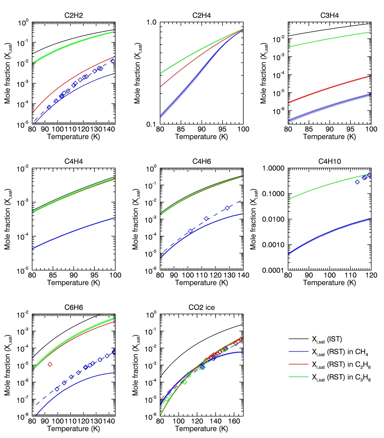
Figure 9: Saturation mole fraction of Titan’s “non-polar solids” (hydrocarbons and carbon dioxide ice) in Titan’s liquids computed using the RST and IST, and different Rackett equations (see Section C.1). The darkest curves represent $X_{i,sat}$ evaluated by Equation 24 with the $Z_{\rm RA}$ parameter. Diamonds are experimental values collected for C₄H₁₀ (Brew, 1977; Kuebler and McKinley, 1975), C₂H₂ (Neumann and Mann, 1969), C₄H₆ (Preston et al., 1971), C₆H₆ (von Szalghary, 1972; Luks et al., 1981; Kuebler and McKinley, 1995; Malaska and Hodyss, 2014) and CO₂ (Clark and Din, 1953; Davis et al., 1962; Cheung and Zander, 1968; Preston et al., 1971) in the corresponding liquids. Dashed lines are empirical power fits of the experimental points (with $R^{2}>0.98$).

The solubilities are given for a wide range of temperatures in Figures 9 (non-polar molecules) and 10 (polar molecules), ontop of which we also reported experimental data points gathered from the literature, fitted by an empirical power law ($R^{2}>0.98$) in order to extrapolate the experimental values at low temperatures for comparison.

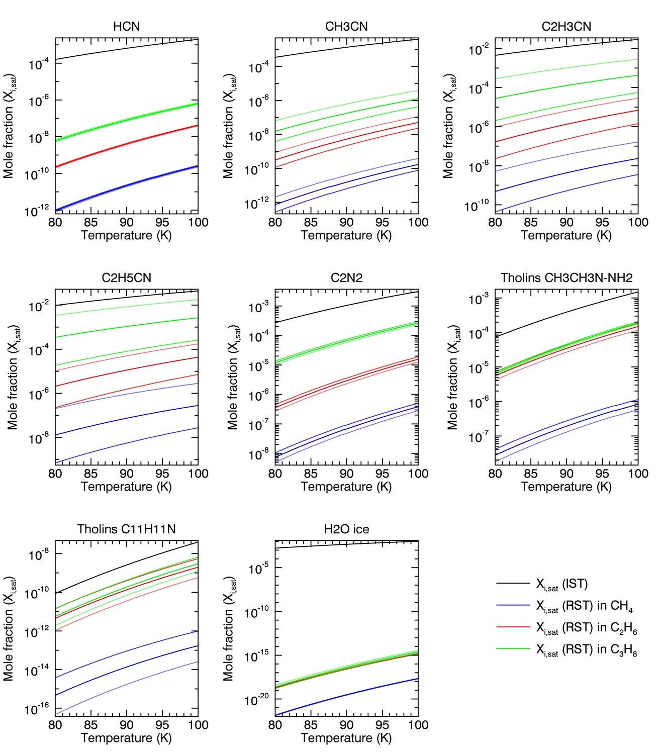
Figure 10: Same as Figure 9 but for Titan’s polar solids (nitriles and water ice).

The IST hypothesis provides a first estimate of the solubility, as seen in Figures 9 and 10. It does not consider the different behavior of the solutes in the different solvents, but presents the advantage of not depending on approximate calculations of the activity coefficients of each species. According to this theory, all simple hydrocarbons would thus be rather solubles at low temperatures, the least soluble being nitriles and C₆H₆.

The RST hypothesis provides a second estimate and shows that solids are less soluble in methane than in ethane and propane. Whatever the liquid, simple nitriles generally show an increase in solubility with a higher number of C atoms in their carbon chain. C₂H₄, C₄H₁₀ and C₂H₂ are the most soluble compounds again, joined by C₄H₄, C₄H₆, CO₂, C₃H₄ and finally C₆H₆. Nitriles are the least soluble compounds. At cryogenic temperatures ($<100$ K), the simulated solubilities are in good agreement with the power fits of experimental data (with the exception of n-butane, which shows a higher solubility in experiments). It is also worth noting that recent solubility experiments of benzene in liquid ethane have been performed at 94 K by Malaska and Hodyss (2014). The $X_{i,\rm sat}$ for benzene in ethane they determined experimentally ($1.11\pm 0.09\times 10^{-5}$) is also quite close to our theoretical value computed using the RST at 94 K ($4.42\times 10^{-5}$), though slightly lower. This difference is probably due to the dissolution of nitrogen into liquid ethane during the experiment, which tends to lower the solubility of benzene. Benzene also reached saturation so quickly in liquid ethane (in less than 2h) (Malaska and Hodyss, 2014), compared to the timescales considered in the present work, that dissolution can be assumed instantaneous. Finally, as expected, the solubility of water ice is unconstrained given the considerable range between IST and RST estimates (about a factor 10¹⁷), but is probably low.

Solubilities calculated using the IST and RST are also given at 91.5 K in Table 8 along with those gathered from our empirical fits of experimental data and the literature. The fits of experimental data are quite consistent with our RST values. Previous studies document the solubility of pure solids in liquid mixtures in equilibrium with the atmosphere (thus composed of methane, ethane, propane and/or nitrogen) at various temperatures. Direct comparisons are therefore tentative, since the liquid composition, temperatures and the thermodynamic parameters sources are heterogeneous. Nitrogen tends to decrease the solubility of solids in liquids while ethane and propane tend to increase it. It should be noted that the solubility of hydrocarbons is quite in agreement between our study and others (Raulin, 1987; Dubouloz et al., 1989; Glein and Shock, 2013) but the solubility of nitriles appears lower in our simulations than in previous ones (Raulin, 1987; Dubouloz et al., 1989; Cordier et al., 2013a), for which they lie between our IST and RST estimates.

Appendix C Molar volumes of solvents and solutes

If the density of a compound at a given temperature ($T$) is known from experimental data, it is straightforward to derive its molar volume $V_{{\rm m},i}(T)$, as follows:

$$V_{{\rm m},i}(T)=M_{i}/\rho_{i}(T)\qquad\textrm{[m${}^{3}$/mol]}$$ (22)

This is the case for water ice (Loerting et al., 2011) and minerals (Lide, 2010). However, experimentally determined densities for solids and liquids at the very low temperatures relevant to Titan are rather rare. We describe two complimentary techniques to evaluate the molar volumes of solids and liquids.

C.1 Subcooled liquid molar volumes

We first evaluate molar volumes at a given temperature $T$ using the Rackett equation (Spencer and Danner, 1972; Poling et al., 2007). This method is designed to estimate the saturated subcooled liquid molar volumes of pure hydrocarbons and organic solvents ($V_{{\rm m},i}^{L}$).

$$V_{{\rm m},i}^{L}=\frac{R\,T_{{\rm c},i}}{P_{{\rm c},i}}Z_{c,i}\,^{\left[1+(1-T_{\rm r,i})^{2/7}\right]}\qquad\textrm{[m${}^{3}$/mol]}$$ (23)

$R$ is the ideal gas constant ($=8.3144621$ J/mol/K), $T_{\rm c}$ and $P_{\rm c}$ are the critical temperature (in K) and pressure (in Pa or J/m³) respectively, $Z_{c}$ is the critical compressibility factor, similar to the Rackett parameter ($Z_{\rm RA}=0.29056-0.08775\omega$, $\omega$ being the accentric factor, see Poling et al. (2007) for more details) and $T_{\rm r}$ the reduced temperature ($T_{\rm r,i}=T/T_{\rm c,i}$). All these parameters are given in Table 9. An alternative form of this equation is given by:

$$V_{{\rm m},i}^{L}=V_{c,i}\,Z_{c,i}\,^{\left(1-T_{\rm r,i}\right)^{2/7}}\qquad\textrm{[m${}^{3}$/mol]}$$ (24)

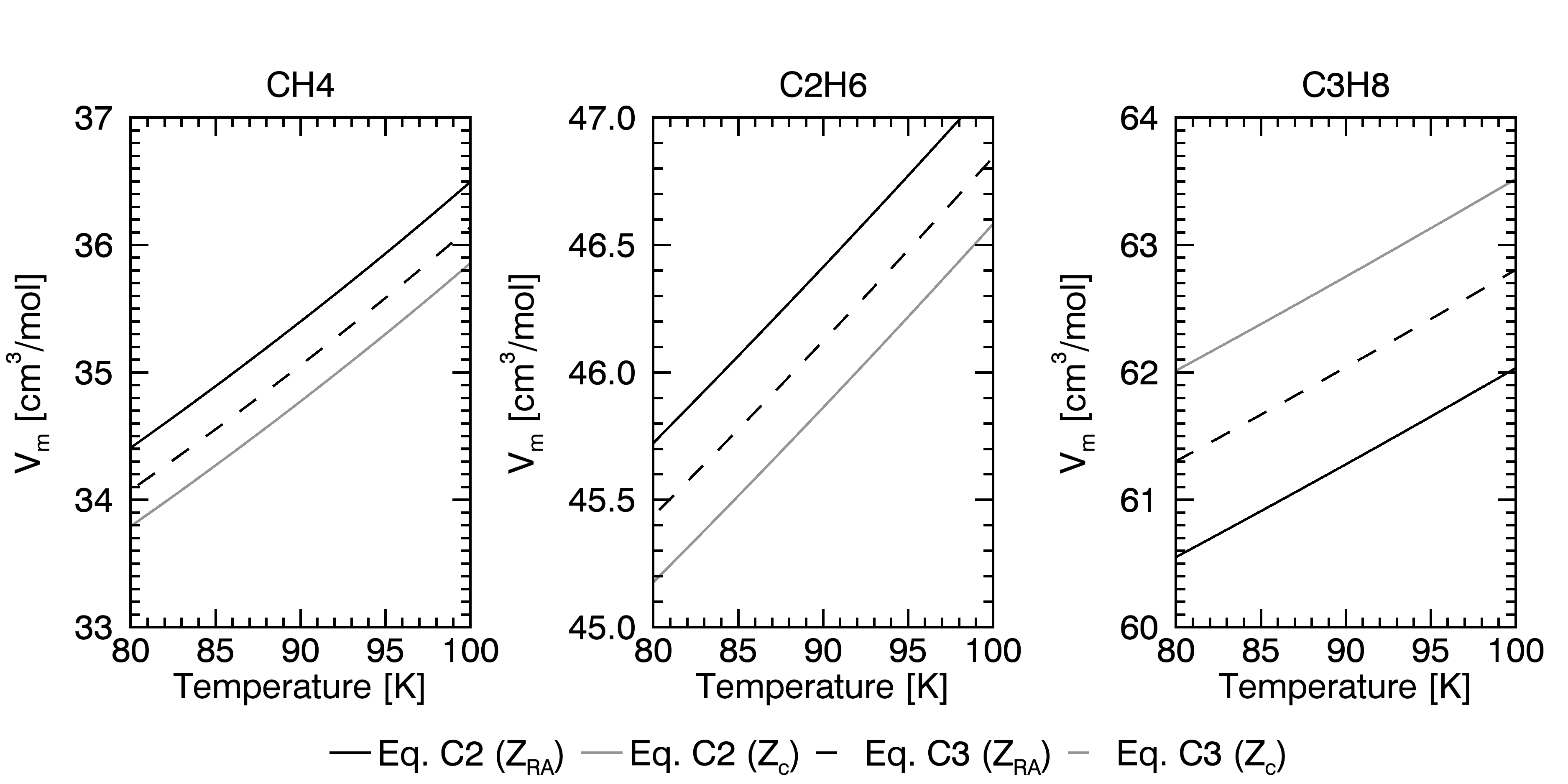
Figure 11: Differences in the calculated molar volumes of Titan’s liquids due to the use of different Rackett equations and compressibility factors.

We investigated uncertainties in the molar volumes computed using the Rackett equations (23 and 24), with the two different parameters ($Z_{\rm RA}$, taken from database or computed using the accentric factor, and $Z_{c}$, computed from the ideal gas equation at the critical point). The results are reported in Table 10 and Figures 11 (liquids), 12 (non-polar solids) and 13 (polar solids). Differences in molar volumes are only significant for nitriles, going up to $2\sigma<24$ cm³/mol for propionitrile. To reduce possible over or underestimates for nitriles molar volumes and solubilities, we use Equation 24 with $Z_{\rm RA}$, which is our “intermediate” case and also the most accurate estimates of $V_{{\rm m},i}^{L}$ (Poling et al., 2007).

C.2 Titan’s solids molar volumes

The solid molar volumes were determined from crystal structures available in the literature (Dulmage and Lipscomb, 1951; Dietrich et al., 1975; Simon and Peters, 1980; Refson and Pawley, 1986; Antson et al., 1987; Etters and Kuchta, 1989; McMullan et al., 1992; Craven et al., 1993). The CH₃CN, HCN, C₄H₁₀ and C₂H₂ have a temperature dependent polymorphism. For each of these compounds, the selected crystal structure corresponds to the one observed at the temperature of Titan’s surface (i.e. 90 - 95 K). Except for CH₃CN, the cell volume was experimentally determined for different temperatures. A second order polynomial was used to fit the cell volume as a function of the temperature to extrapolate them at Titan’s temperatures (90 - 95 K).

Since the pressure on Titan (around 1.5 bar) is not the same as on Earth (1 bar) where the crystal cell volume were determined, we checked the influence pressure on molar volumes by calculations based on the Density Functional Theory (DFT) using the VASP 5.3 package. Cell volumes of each compound were optimized using vdW-DF2 (Lee et al., 2010; Klimeš et al., 2011) functional involving a non-local kernel for the electronic correlation energy calculation. This functional allows to reproduce dispersion interactions (such as Van der Waals interactions) which are major inter-molecular interaction encountered in molecular crystals. The $E_{\rm ncut}$ value, defining the basis set size, was fixed to 800 eV in order to suppress Pulay’s stress. The k-points sampling was done with a $12\times 12\times 12$ Monkhorst-Pack grid. The core electrons were described with the projector-augmented plane wave (PAW) approach. Calculations were performed with and without static pressure (set to 100 bar) to compare cell volumes. The larger variation was observed for C₄H₁₀, with a volume decrease of 0.44 % upon pressure. This is reasonably low to conclude that cell volumes measured on Earth (P=1 bar) should be very similar to the ones on Titan (P=1.5 bar).

We reported on Figures 12 and 13 the predicted crystalline molar volumes ontop of the experimental and Rackett values (individual values also given in Table 11). Overall, we get a quite good agreement between all these estimates. We estimate the solid molar volumes at 91.5 K using a simple empirical linear fit between experimental and predicted points. The Rackett method is used to give an approximate molar volume for the solids for which we do not have experimental data.

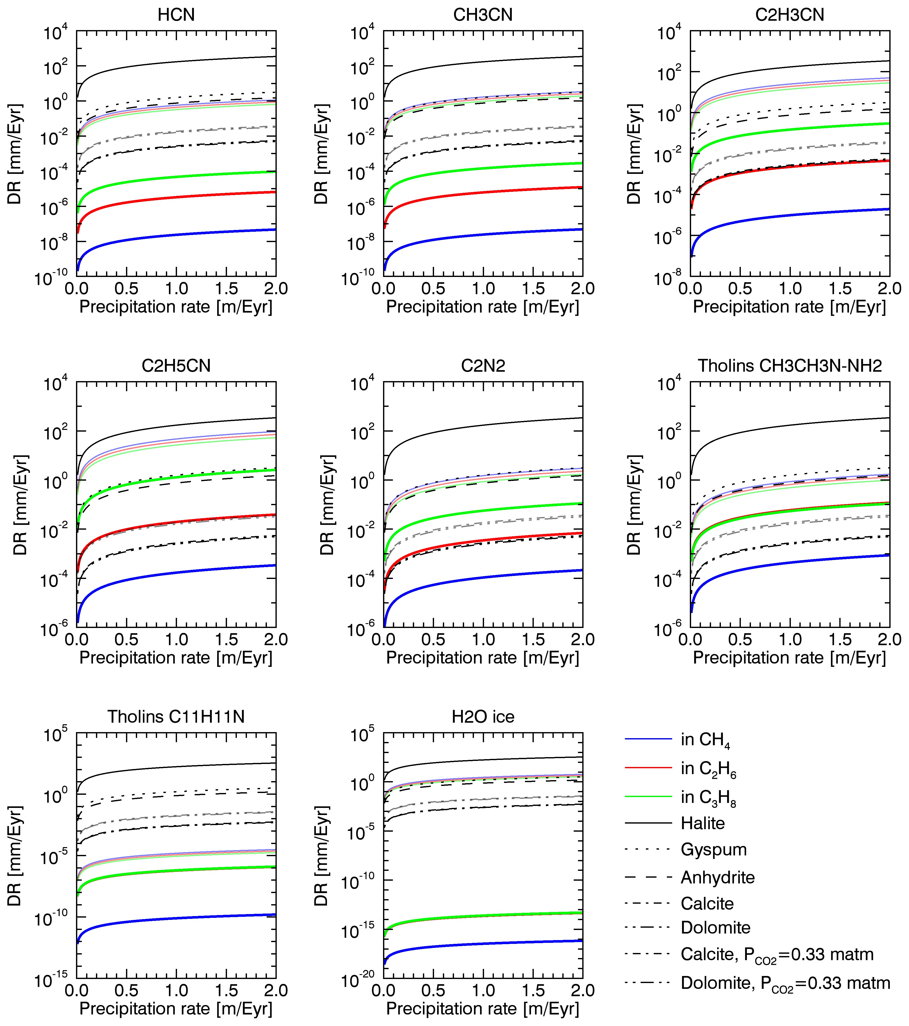
Figure 4: Same as Figure 3 but for polar molecules (nitriles and water ice).

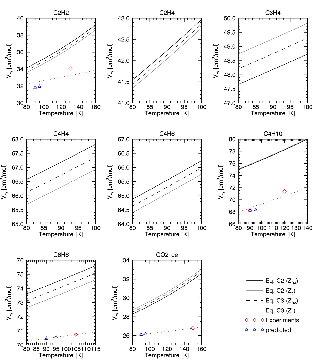
Figure 12: Same as Figure 11 but for “non-polar” solids (hydrocarbons and carbon dioxide ice). Red and blue diamonds are experimental and predicted values respectively. Sources: C₄H₁₀ (Refson and Pawley, 1986), C₂H₂ (McMullan et al., 1992), C₆H₆ (Craven et al., 1993) and CO₂ (Simon and Peters, 1980).

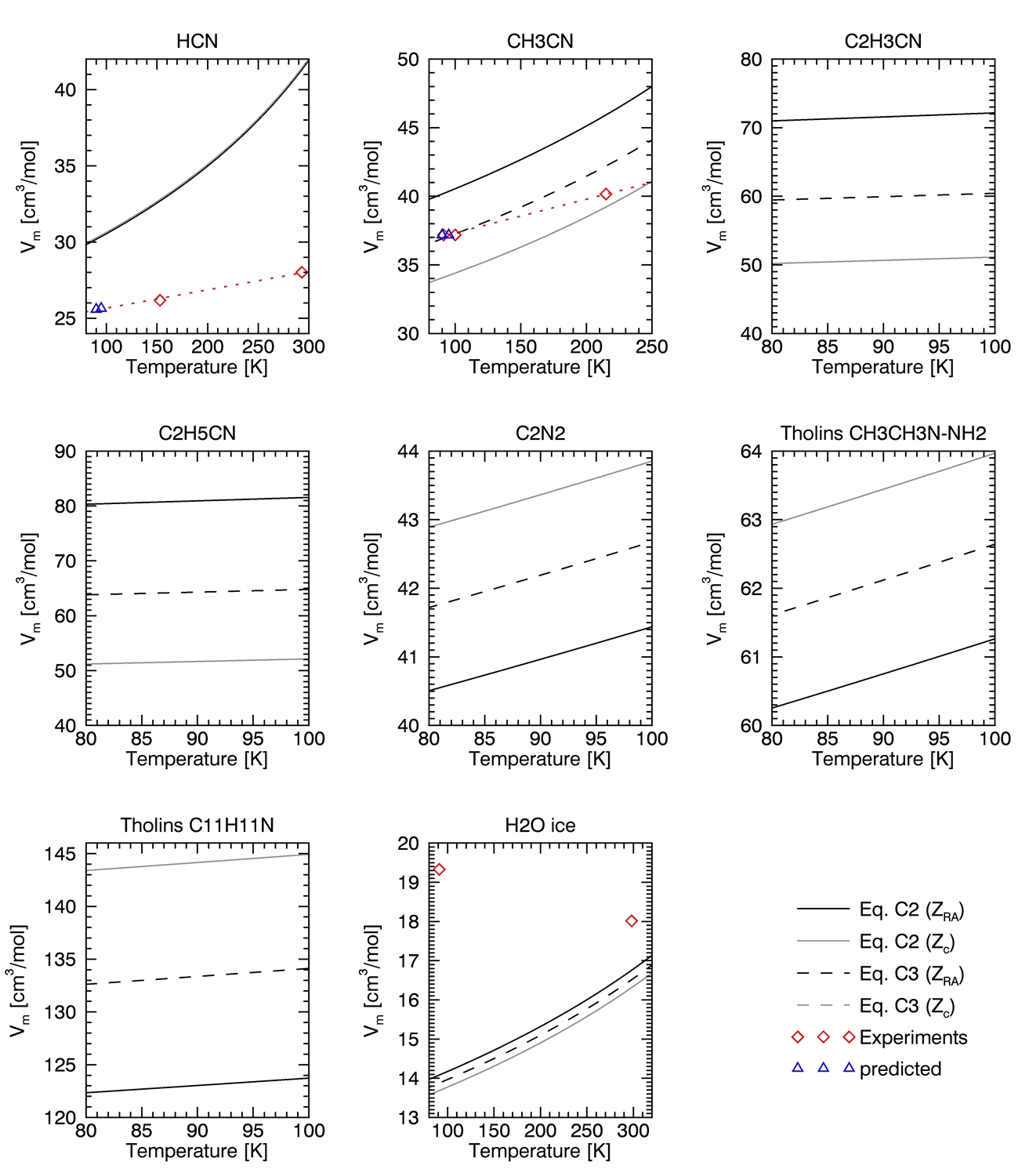
Figure 13: Same as Figure 12 but for polar solids (nitriles and water ice). Sources: HCN (Dulmage and Lipscomb, 1951), CH₃CN (Barrow, 1981; Antson et al., 1987) and H₂O (Loerting et al., 2011).

Table 1: Production rates (in molecules/cm²/s) of simple solid organics in Titan’s atmosphere derived from several photochemical models. Not reported here is the production rate of tholins, estimated by Cabane et al. (1992), Rannou et al. (2003) and Krasnopolsky (2009) to be between 0.2 and 7 kg/cm²/GEyr (Giga Earth year). The list of compound names is available in Appendix A. Y84: Yung et al. (1984), T95: Toublanc et al. (1995), L96: Lara et al. (1996), W04: Wilson and Atreya (2004), L08: Lavvas et al. (2008a, b), K09: Krasnopolsky (2009).

	Y84	T95	L96	W04	L08	K09
C2H6	5.80$\times 10^{9}$	1.50$\times 10^{10}$	1.41$\times 10^{9}$	1.60$\times 10^{9}$	4.10$\times 10^{9}$	1.16$\times 10^{9}$
C3H8	1.40$\times 10^{8}$	5.40$\times 10^{8}$	3.14$\times 10^{7}$	3.30$\times 10^{7}$	3.70$\times 10^{8}$	2.17$\times 10^{8}$
C4H10	2.30$\times 10^{7}$	8.80$\times 10^{7}$		3.00$\times 10^{7}$		7.02$\times 10^{5}$
C2H2	1.20$\times 10^{9}$	1.10$\times 10^{9}$	9.28$\times 10^{8}$	3.70$\times 10^{8}$	3.20$\times 10^{8}$	3.22$\times 10^{8}$
C2H4				9.30$\times 10^{7}$	6.00$\times 10^{7}$
C3H4						2.64$\times 10^{6}$
C4H4						1.57$\times 10^{4}$
C4H6				6.50$\times 10^{4}$		1.71$\times 10^{7}$
C6H6				4.60$\times 10^{5}$	2.10$\times 10^{5}$	1.08$\times 10^{6}$
HCN	2.00$\times 10^{8}$	1.00$\times 10^{8}$	8.00$\times 10^{7}$	2.10$\times 10^{6}$	3.20$\times 10^{8}$	1.54$\times 10^{8}$
HC3N	1.70$\times 10^{7}$		3.73$\times 10^{7}$	1.30$\times 10^{7}$	9.20$\times 10^{6}$	1.26$\times 10^{7}$
C2N2	1.20$\times 10^{7}$		2.89$\times 10^{4}$	2.00$\times 10^{6}$	2.60$\times 10^{4}$	3.52$\times 10^{6}$
C4N2			7.20$\times 10^{6}$	9.70$\times 10^{5}$	1.90$\times 10^{6}$
CH3CN			6.61$\times 10^{5}$	3.40$\times 10^{4}$	1.70$\times 10^{7}$	1.27$\times 10^{7}$
C2H3CN				1.60$\times 10^{7}$	2.80$\times 10^{5}$	1.62$\times 10^{7}$
C2H5CN						8.00$\times 10^{5}$

Table 2: Solutional denudation rates in mm/Eyr for terrestrial minerals at 298.15 K and under various climatic conditions (CO₂ content and precipitation rates). All values correspond to the EST hypothesis except those for halite (IST).

Name	$\tau=30$ cm/Eyr	$\tau=1$ m/Eyr
	Dissolution by dissociation
Halite	50.643	167.122
Gyspum	0.504	1.662
Anhydrite	0.224	0.740
Calcite	8.55$\times 10^{-4}$	2.82$\times 10^{-3}$
Dolomite	7.84$\times 10^{-4}$	2.59$\times 10^{-3}$
	Acid dissolution
Calcite, $PCO_{2}$ = 0.33 matm	0.006	0.020
Dolomite, $PCO_{2}$ = 0.33 matm	0.005	0.017
Calcite, $PCO_{2}$ = 0.01 atm	0.020	0.066
Dolomite, $PCO_{2}$ = 0.01 atm	0.017	0.057
Calcite, $PCO_{2}$ = 0.11 atm	0.047	0.156
Dolomite, $PCO_{2}$ = 0.11 atm	0.040	0.132

Table 3: Timescales required to dissolve 100 meters of a surface organic layer (composition given by photochemistry in the atmosphere) in liquid methane according to the precipitation rates of Schneider et al. (2012).

Latitude	IST		RST
	min (kEyrs)	max (kEyrs)	min (kEyrs)	max (MEyrs)
80∘N	1.6	20.9	3.9	22.1
70∘N	3.5	45.2	8.5	47.8
60∘N	7.7	99.0	18.7	104.6
60∘S	27.6	354.9	67.1	375.1
70∘S	4.1	53.2	10.1	56.2
80∘S	1.8	23.7	4.5	25.0

Table 4: Thermodynamic and physical parameters of minerals, water and ions considered in the dissolution reactions, collected from the literature (Lide, 2010; Langmuir, 1997; Ford and Williams, 2007; Brezonik and Arnold, 2011; White, 2013).

Name	Formula	$M_{i}$	$z_{i}$	$a_{i}$	$b_{i}$	$\Delta_{\rm f}G_{i}^{\circ}$	$\Delta_{\rm f}H_{i}^{\circ}$
		[g/mol]		[Å]	[kg/mol]	[kJ/mol]	[kJ/mol]
minerals
calcite	CaCO3	100.087	0	-	-	-1129.1	-1207.6
dolomite	CaMg(CO3)2	184.401	0	-	-	-2161.7	-2324.5
gypsum	CaSO4.2H2O	172.171	0	-	-	-1797.2	-2022.6
anhydrite	CaSO4	136.141	0	-	-	-1321.7	-1434.1
halite	NaCl	58.443	0	-	-	-384.1	-411.2
aqueous species
chlore	Cl-	35.460	$-1$	3.71	0.01	-131.3	-167.2
sodium	Na+	22.990	$+1$	4.32	0.06	-261.9	-240.1
hydroxyl	OH-	17.007	$-1$	10.65	0.21	-157.3	-230
hydrogen	H+	1.008	$+1$	4.78	0.24	0	0
calcium	Ca2+	40.080	$+2$	4.86	0.15	-553.54	-542.83
magnesium	Mg2+	24.320	$+2$	5.46	0.22	-454.8	-466.8
sulfate	SO${}_{4}^{2-}$	96.060	$-2$	5	-0.04	-744.6	-909.2
carbonate	CO${}_{3}^{2-}$	60.010	$-2$	5.4	0	-527.9	-677.1
bicarbonate	HCO3-	61.020	$-1$	5.4	0	-586.8	-692
carbonic acid	H2CO3	62.025	0	-	-	-623.2	-699.7
solvent and gas
water	H2O	18.015	0	-	-	-237.18	-285.83
carbon dioxide	CO2	44.010	0	-	-	-394.4	-393.51

Table 5: Thermodynamic constants of dissociation and dissolution reactions in standard conditions (at 25^∘C and 1 atm).

Reaction	Equations	$\Delta_{\rm r}G^{\circ}$	$\Delta_{\rm r}H^{\circ}$	$K_{eq}$	${\rm p}K_{eq}$	Equilibrium constant expression
		[kJ/mol]	[kJ/mol]
Pure dissociation reactions for minerals
gypsum dissociation	CaSO4.2H2O $\iff$ Ca2+ + SO${}_{4}^{2-}$ + 2H2O	24.70	-1.09	4.71$\times 10^{-5}$	4.327	$K_{gd}=(Ca^{2+})(SO_{4}^{2-})$
anhydrite dissociation	CaSO4 $\iff$ Ca2+ + SO${}_{4}^{2-}$	23.56	-17.93	7.46$\times 10^{-5}$	4.128	$K_{ad}=(Ca^{2+})(SO_{4}^{2-})$
halite dissociation	NaCl $\iff$ Na+ + Cl-	-9.10	3.90	39.29	-1.594	$K_{hd}=(Na^{+})(Cl^{-})$
calcite dissociation	CaCO3 $\iff$ Ca2+ + CO${}_{3}^{2-}$	47.36	-12.53	5.05$\times 10^{-9}$	8.297	$K_{cd}=(Ca^{2+})(CO_{3}^{2-})$
dolomite dissociation	CaMg(CO3)2 $\iff$ Ca2+ + Mg2+ + 2CO${}_{3}^{2-}$	97.56	-39.33	8.10$\times 10^{-18}$	17.092	$K_{dd}=(Ca^{2+})(Mg^{2+})(CO_{3}^{2-})^{2}$
Secondary dissociation reactions and dissolution reactions for carbonates dissolution
CO2 dissolution	CO2 + H2O $\iff$ H2CO${}_{3}^{\circ}$	8.38	-20.36	3.40$\times 10^{-2}$	1.468	$K_{CO_{2}}=(H_{2}CO_{3}^{\circ})/P_{CO_{2}}$
carbonic acid dissociation	H2CO${}_{3}^{\circ}$ $\iff$ H+ + HCO${}_{3}^{-}$	36.40	7.70	4.20$\times 10^{-7}$	6.377	$K_{1}=(H^{+})(HCO_{3}^{-})/(H_{2}CO_{3}^{\circ})$
bicarbonate dissociation	H+ + CO${}_{3}^{2-}$ $\iff$ HCO${}_{3}^{-}$	58.90	14.90	4.80$\times 10^{-11}$	10.319	$K_{2}=(HCO_{3}^{-})/(H^{+})(CO_{3}^{2-})$
calcite dissolution	CaCO3 + H2O + CO2 $\iff$ Ca2+ + 2 HCO${}_{3}^{-}$	33.24	-40.09	1.50 $\times 10^{-6}$	5.823	$K_{cal}=(Ca^{2+})(HCO3^{-})^{2}/P_{CO_{2}}$
dolomite dissolution	CaMg(CO${}_{3})_{2}$ + 2H2O + 2CO2 $\iff$ Ca2+ + Mg2+ + 4 HCO${}_{3}^{-}$	69.32	-94.45	7.17 $\times 10^{-13}$	12.144	$K_{dol}=(Ca^{2+})(Mg^{2+})(HCO3^{-})^{4}/P_{CO_{2}}^{2}$

Table 6: Molalities in mol/kg of solvent of minerals in water at 25^∘C according to the Ideal and the Electrolyte Solutions Theories. $P_{CO_{2}}=0.33$ matm refers to normal dry air (Langmuir, 1997) while $P_{CO_{2}}=0.01$ atm more refers to tropical climate environments (Fleurant et al., 2008), which actually could even reach considerable CO₂ content in the soils of up to $P_{CO_{2}}=0.11$ atm (Ford and Williams, 2007).

Name	IST	EST
	Dissolution by dissociation
Halite	6.27	6.27
Gyspum	8.63$\times 10^{-3}$	2.26$\times 10^{-2}$
Anhydrite	6.86$\times 10^{-3}$	1.62$\times 10^{-2}$
Calcite	7.10$\times 10^{-5}$	7.72$\times 10^{-5}$
Dolomite	3.77$\times 10^{-5}$	4.11$\times 10^{-5}$
	Acid dissolution
Calcite, PCO2 = 0.33 matm	4.99$\times 10^{-4}$	5.42$\times 10^{-4}$
Dolomite, PCO2 = 0.33 matm	2.59$\times 10^{-4}$	2.76$\times 10^{-4}$
Calcite, PCO2 = 0.01 atm	1.55$\times 10^{-3}$	1.80$\times 10^{-3}$
Dolomite, PCO2 = 0.01 atm	8.09$\times 10^{-4}$	8.99$\times 10^{-4}$
Calcite, PCO2 = 0.11 atm	3.46$\times 10^{-3}$	4.28$\times 10^{-3}$
Dolomite, PCO2 = 0.11 atm	1.80$\times 10^{-3}$	2.09$\times 10^{-3}$

Table 7: Melting and boiling points thermodynamic constants of Titanian materials. Data gathered from Lide (2010) and Yaws (1996). The melting properties of C₁₁H₁₁N have been taken in Chirico et al. (2007).

Formula	$T_{\rm m}$	$\Delta_{\rm m}H^{\circ}$	$T_{b}$	$\Delta_{\rm v}H^{\circ}$
	[K]	[kJ/mol]	[K]	[kJ/mol]
CH4	90.680	0.940	111.670	8.190
C2H6	90.360	0.582	184.570	14.690
C3H8	85.460	3.500	232.040	19.040
C4H10	134.850	4.660	272.660	22.440
C2H2	192.450	4.105	188.450	16.674
C2H4	104.000	3.350	169.380	13.530
C3H4	170.450	5.349	249.950	22.185
C4H4	227.600	7.687	278.250	22.470
C4H6	164.240	7.980	268.740	22.470
C6H6	278.640	9.870	353.240	30.720
HCN	259.860	8.406	298.850	26.896
C2N2	245.320	8.110	252.100	23.330
CH3CN	229.330	8.160	354.800	29.750
C2H3CN	189.670	6.230	350.450	32.600
C2H5CN	207.150	5.030	350.500	31.810
C2H8N2	215.950	10.070	337.050	28.477
C11H11N	326.650	20.418	538.855	50.005
H2O	273.150	6.010	373.200	40.650
CO2	216.592	9.020	194.600	15.326

Table 8: Saturation mole fractions of Titan’s solids in pure liquid methane, ethane and propane at 91.5 K evaluated using the Ideal Solutions and Regular Solutions Theories compared with our fits at 91.5 K of experimental data and with values taken from the literature. R87: Raulin (1987) (graphical reading), D89: Dubouloz et al. (1989), C13: Cordier et al. (2013b), G13: Glein and Shock (2013), T13: Tan et al. (2013).

Formula	$X_{i}$ (IST)	$X_{i}$ (RST)			Experiments	R87 (RST)		D89 (RST)	C13 (IST)	G13 (MVL)	T13 (PC-SAFT)
	91.5 K	91.5 K			91.5 K	94 K		92.5 K	90 K	90.7 K	90 K	93.7 K
CH4	-	1.00	-	-	1.00	8.60$\times 10^{-1}$	-	7.30$\times 10^{-2}$	-	6.81$\times 10^{-1}$	6.84$\times 10^{-1}$	3.18$\times 10^{-1}$
C2H6	-	-	1.00	-	-	-	9.70$\times 10^{-1}$	9.09$\times 10^{-1}$	-	1.55$\times 10^{-1}$	8.30$\times 10^{-2}$	5.32$\times 10^{-1}$
C3H8	-	-	-	1.00	-	-	-		-	1.55$\times 10^{-2}$	7.80$\times 10^{-3}$	7.20$\times 10^{-2}$
N2	-	-	-	-	-	1.40$\times 10^{-1}$	3.00$\times 10^{-2}$	1.80$\times 10^{-2}$	-	1.48$\times 10^{-1}$	2.21$\times 10^{-1}$	6.89$\times 10^{-2}$
C4H10	1.40$\times 10^{-1}$	1.51$\times 10^{-3}$	1.39$\times 10^{-1}$	1.40$\times 10^{-1}$	-	-	-	-	1.22$\times 10^{-1}$	-	-	-
C2H2	5.90$\times 10^{-2}$	4.48$\times 10^{-5}$	2.00$\times 10^{-4}$	2.45$\times 10^{-2}$	5.72$\times 10^{-5}$	1.81$\times 10^{-4}$	6.93$\times 10^{-4}$	4.10$\times 10^{-4}$	5.40$\times 10^{-2}$	2.20$\times 10^{-4}$	3.40$\times 10^{-3}$	7.70$\times 10^{-3}$
C2H4	5.89$\times 10^{-1}$	4.02$\times 10^{-1}$	5.33$\times 10^{-1}$	5.88$\times 10^{-1}$	-	1.81$\times 10^{-3}$	4.62$\times 10^{-2}$	-	-	-	-	-
C3H4	3.85$\times 10^{-2}$	2.25$\times 10^{-6}$	2.36$\times 10^{-5}$	1.14$\times 10^{-2}$	-	7.26$\times 10^{-6}$	1.39$\times 10^{-4}$	5.00$\times 10^{-5}$	-	-	-	-
C4H4	2.38$\times 10^{-3}$	1.64$\times 10^{-4}$	2.05$\times 10^{-3}$	2.16$\times 10^{-3}$	-	-	-	-	-	-	-	-
C4H6	9.60$\times 10^{-3}$	3.57$\times 10^{-5}$	7.57$\times 10^{-3}$	8.06$\times 10^{-3}$	4.85$\times 10^{-5}$	3.27$\times 10^{-5}$	2.77$\times 10^{-4}$	-	-	-	-	-
C6H6	1.64$\times 10^{-4}$	5.32$\times 10^{-8}$	3.11$\times 10^{-5}$	3.76$\times 10^{-5}$	1.59$\times 10^{-7}$	3.63$\times 10^{-7}$	9.24$\times 10^{-6}$	-	2.20$\times 10^{-4}$	-	-	-
HCN	7.78$\times 10^{-4}$	3.25$\times 10^{-11}$	5.90$\times 10^{-9}$	1.14$\times 10^{-7}$	-	7.26$\times 10^{-7}$	2.31$\times 10^{-5}$	8.50$\times 10^{-6}$	6.46$\times 10^{-4}$	-	-	-
C2N2	1.25$\times 10^{-3}$	8.96$\times 10^{-8}$	3.83$\times 10^{-6}$	8.30$\times 10^{-5}$	-	1.09$\times 10^{-7}$	2.77$\times 10^{-6}$	1.40$\times 10^{-6}$	-	-	-	-
CH3CN	1.59$\times 10^{-3}$	2.31$\times 10^{-11}$	7.64$\times 10^{-9}$	2.42$\times 10^{-7}$	-	2.18$\times 10^{-6}$	2.77$\times 10^{-5}$	6.30$\times 10^{-5}$	3.73$\times 10^{-3}$	-	-	-
C2H3CN	1.44$\times 10^{-2}$	5.75$\times 10^{-9}$	1.74$\times 10^{-6}$	1.54$\times 10^{-4}$	-	-	-	2.20$\times 10^{-5}$	-	-	-	-
C2H5CN	2.49$\times 10^{-2}$	9.28$\times 10^{-8}$	1.41$\times 10^{-5}$	1.25$\times 10^{-3}$	-	2.18$\times 10^{-6}$	3.70$\times 10^{-5}$	8.90$\times 10^{-5}$	-	-	-	-
C2H8N2	4.87$\times 10^{-4}$	2.46$\times 10^{-7}$	4.41$\times 10^{-5}$	5.44$\times 10^{-5}$	-	-	-	-	-	-	-	-
C11H11N	4.07$\times 10^{-9}$	2.08$\times 10^{-14}$	2.09$\times 10^{-10}$	2.94$\times 10^{-10}$	-	-	-	-	-	-	-	-
H2O	5.23$\times 10^{-3}$	6.17$\times 10^{-20}$	5.50$\times 10^{-17}$	7.98$\times 10^{-17}$	-	1.81$\times 10^{-15}$	3.24$\times 10^{-12}$	-	-	-	-	-
CO2	1.06$\times 10^{-3}$	3.29$\times 10^{-5}$	1.23$\times 10^{-5}$	1.32$\times 10^{-5}$	2.68$\times 10^{-5}$	7.26$\times 10^{-5}$	3.24$\times 10^{-5}$	1.20$\times 10^{-5}$	8.72$\times 10^{-4}$	-	-	-

Table 9: Critical properties of Titanian materials (Lide, 2010). The Rackett parameters ($Z_{\rm RA}$) have been gathered from the CHemical and Engineering Research Information Center (CHERIC) database (http://www.cheric.org/research/kdb/hcprop/cmpsrch.php) and from Infotherm (http://www.infotherm.com/servlet/infothermSearch). The compressibility factors ($Z_{c}$) have been calculated for comparison with $Z_{\rm RA}$. The critical properties of cyanogen and our tholins analogues (1-1 dimethyl-hydrazine C₂H₈N₂, as suggested in Cordier et al. (2013b), based on the experiments of Quirico et al. (2008), and quinoline C₁₁H₁₁N, as sugested by Coll et al. (1995)) have been collected in Yaws (1996).

Formula	$M$	$T_{c}$	$P_{c}$	$V_{c}$	$Z_{\rm RA}$	$Z_{c}$
	[g/mol]	[K]	[MPa]	[cm3/mol]
CH4	16.043	190.564	4.599	98.600	0.289	0.286
C2H6	30.069	305.320	4.872	145.500	0.281	0.279
C3H8	44.096	369.830	4.248	203.000	0.277	0.280
C4H10	58.122	425.160	3.787	255.000	0.273	0.273
C2H2	26.037	308.300	6.138	112.200	0.271	0.269
C2H4	28.053	282.340	5.041	131.000	0.282	0.281
C3H4	40.064	402.000	5.630	163.500	0.272	0.275
C4H4	52.075	455.600	4.860	218.710	0.282	0.281
C4H6	54.091	425.000	4.320	221.000	0.271	0.270
C6H6	78.112	562.050	4.895	256.000	0.270	0.268
HCN	27.026	456.700	5.390	139.000	0.197	0.197
C2N2	53.034	399.900	6.303	144.520	0.266	0.274
CH3CN	41.042	545.500	4.850	171.000	0.199	0.183
C2H3CN	53.063	536.000	4.559	214.061	0.261	0.219
C2H5CN	55.079	561.300	4.260	229.000	0.263	0.209
C2H8N2	60.098	522.200	5.400	218.241	0.265	0.271
C11H11N	157.212	775.100	3.353	514.500	0.247	0.268
H2O	18.015	647.140	22.064	56.000	0.233	0.230
CO2	40.010	304.130	7.375	94.000	0.272	0.274

Table 10: Estimated subcooled liquid molar volumes (in cm³/mol) and associated mass densities for our best molar volume estimates (in g/cm³, for Eq. 24 with $Z_{\rm RA}$) for Titan’s solids and liquids, evaluated using the Rackett equations and parameters at 91.5 K.

Formula	Eq. 23	Eq. 23	Eq. 24	Eq. 24	$2\sigma$	$\rho$
	($Z_{\rm RA}$)	($Z_{c}$)	($Z_{\rm RA}$)	($Z_{c}$)	($Z_{\rm RA}$)
CH4	35.557	34.928	35.212	34.928	0.517	0.456
C2H6	46.520	45.968	46.229	45.968	0.456	0.650
C3H8	61.390	62.865	62.153	62.865	1.219	0.710
C4H10	75.882	75.978	75.932	75.978	0.080	0.766
C2H2	34.753	34.185	34.453	34.185	0.469	0.756
C2H4	42.344	42.147	42.240	42.147	0.162	0.664
C3H4	48.267	49.354	48.828	49.354	0.898	0.821
C4H4	67.280	66.398	66.824	66.398	0.729	0.779
C4H6	65.652	65.175	65.405	65.175	0.394	0.827
C6H6	74.256	73.269	73.748	73.269	0.817	1.059
HCN	30.232	30.323	30.279	30.323	0.075	0.893
C2N2	41.034	43.436	42.263	43.436	1.987	1.255
CH3CN	40.219	34.105	36.956	34.105	5.041	1.111
C2H3CN	71.655	50.733	60.016	50.733	17.199	0.884
C2H5CN	81.023	51.731	64.373	51.731	24.046	0.856
C2H8N2	60.828	63.522	62.197	63.522	2.230	0.966
C11H11N	123.135	144.275	133.476	144.275	17.564	1.178
H2O	14.087	13.692	13.884	13.692	0.327	1.298
CO2	28.789	29.225	29.017	29.225	0.360	1.379

Table 11: Subcooled liquid molar volumes (in cm³/mol) and associated mass densities (in g/cm³) of Titan’s solids estimated using the Rackett equation 24 with $Z_{\rm RA}$ at 91.5 K compared to the solid molar volumes (in cm³/mol) and associated mass densities (in g/cm³) computed from an empirical linear fit between predictions of the model and experimental data for some Titanian materials.

Name	Formula	$V_{\rm m}^{L}$ (Eq. 24, $Z_{\rm RA}$)	$V_{\rm m}^{S}$ (fit)	$2\sigma$	$\rho^{L}$	$\rho^{S}$
n-butane	C4H10	75.932	68.737	7.195	0.766	0.846
acetylene	C2H2	34.453	32.471	1.982	0.756	0.802
benzene	C6H6	73.748	70.487	3.261	1.059	1.108
hydrogen cyanide	HCN	30.279	25.562	4.717	0.893	1.057
acetonitrile	CH3CN	36.956	37.122	0.166	1.111	1.106
water ice Ih	H2O	13.884	19.329	5.446	1.298	0.932
carbon dioxide ice	CO2	29.017	26.109	2.909	1.379	1.532

References

- Acocella (2007) Acocella, V. (2007), Understanding caldera structure and development: An overview of analogue models compared to natural calderas, Earth-Science Reviews, 85(3-4), 125 – 160, doi:10.1016/j.earscirev.2007.08.004.
- Aharonson et al. (2009) Aharonson, O., A. G. Hayes, J. I. Lunine, R. D. Lorenz, M. D. Allison, and C. Elachi (2009), An asymmetric distribution of lakes on Titan as a possible consequence of orbital forcing, Nature Geoscience, 2, 851–854, doi:10.1038/ngeo698.
- Antson et al. (1987) Antson, O., K. Tilli, and N. Andersen (1987), Neutron Powder Diffraction Study of Deuterated -Acetonitrile, Acta Crystallographica Section B, 43, 296–301, doi:10.1107/S0108768187097866.
- Atreya (2007) Atreya, S. K. (2007), Titan’s organic factory, Science, 316(5826), 843–845, doi:10.1126/science.1141869.
- Barnes et al. (2007) Barnes, J. W., R. H. Brown, L. Soderblom, B. J. Buratti, C. Sotin, S. Rodriguez, S. Le Mouélic, K. H. Baines, R. Clark, and P. Nicholson (2007), Global-scale surface variations on Titan seen from Cassini/VIMS, Icarus, 186(1), 242 – 258, doi:10.1016/icarus.2006.08.021.
- Barnes et al. (2009) Barnes, J. W., R. H. Brown, J. M. Soderblom, L. A. Soderblom, R. Jaumann, B. Jackson, S. Le Mouélic, C. Sotin, B. J. Buratti, K. M. Pitman, K. H. Baines, R. N. Clark, P. D. Nicholson, E. P. Turtle, and J. Perry (2009), Shoreline features of Titan’s Ontario Lacus from Cassini/VIMS observations, Icarus, 201(1), 217 – 225, doi:10.1016/j.icarus.2008.12.028.
- Barnes et al. (2011) Barnes, J. W., J. Bow, J. Schwartz, R. H. Brown, J. M. Soderblom, A. G. Hayes, G. Vixie, S. Le Mouélic, S. Rodriguez, C. Sotin, R. Jaumann, K. Stephan, L. A. Soderblom, R. N. Clark, B. J. Buratti, K. H. Baines, and P. D. Nicholson (2011), Organic sedimentary deposits in Titan’s dry lakebeds: Probable evaporite, Icarus, 216(1), 136 – 140, doi:10.1016/j.icarus.2011.08.022.
- Barrow (1981) Barrow, M. (1981), -acetonitrile at 215 K, Acta Crystallographica Section B, 37, 2239–2242, doi:10.1107/S0567740881008510.
- Black et al. (2012) Black, B. A., J. T. Perron, D. M. Burr, and S. A. Drummond (2012), Estimating erosional exhumation on Titan from drainage network morphology, Journal of Geophysical Research, 117, E08,006, doi:10.1029/2012JE004085.
- Bourgeois et al. (2008) Bourgeois, O., T. Lopez, S. Le Mouélic, C. Fleurant, G. Tobie, L. Le Corre, L. Le Deit, C. Sotin, and Y. Bodeur (2008), A surface dissolution/precipitation model for the development of lakes on Titan, based on an arid terrestrial analogue: The pans and calcretes of Etosha, in Lunar and Planetary Science XXXIX, p. 1733.
- Bowen and Johnson (2012) Bowen, M. W., and W. C. Johnson (2012), Late quaternary environmental reconstructions of playa-lunette system evolution on the central High Plains of Kansas, United States, Geological Society of America Bulletin, 124(1), 146–161, doi:10.1130/B30382.1.
- Brew (1977) Brew, T. C. L. (1977), A study on the solubility of heavy hydrocarbons in liquid methane and methane containing mixtures, Master’s thesis, University of Ottawa, Canada.
- Brezonik and Arnold (2011) Brezonik, P., and W. Arnold (2011), Water chemistry: An introduction to the chemistry of natural and engineered aquatic systems, 809 pp., Oxford University Press, Inc., New York.
- Brown et al. (2008) Brown, R. H., L. A. Soderblom, J. M. Soderblom, R. N. Clark, R. Jaumann, J. W. Barnes, C. Sotin, B. Buratti, K. H. Baines, and P. D. Nicholson (2008), The identification of liquid ethane in Titan’s Ontario Lacus, Nature, 454, 607 – 610, doi:10.1038/nature07100.
- Buch (1997) Buch, M. W. (1997), Etosha Pan - The third largest lake in the world ?, Madoqua, 20(1), 49 – 64.
- Buch and Rose (1996) Buch, M. W., and D. Rose (1996), Mineralogy and geochemistry of the sediments of the Etosha Pan Region in northern Namibia: A reconstruction of the depositional environment, Journal of African Earth Sciences, 22(3), 355 – 378, doi:10.1016/0899-5362(96)00020-6.
- Buch and Trippner (1997) Buch, M. W., and C. Trippner (1997), Overview of the geological and geomorphological evolution of the Etosha region, Northern Namibia, Madoqua, 20(1), 65 – 74.
- Cabane et al. (1992) Cabane, M., E. Chassefière, and G. Israel (1992), Formation and growth of photochemical aerosols in Titan’s atmosphere, Icarus, 96(2), 176 – 189, doi:10.1016/0019-1035(92)90071-E.
- Cheung and Zander (1968) Cheung, H., and E. H. Zander (1968), Solubility of carbon dioxide and hydrogen sulfide in liquid hydrocarbons at cryogenic temperatures, Chemical Engineering Progress, 64(88), 34.
- Chevrier et al. (2014) Chevrier, V., S. Singh, D. Nna-Mvondo, D. Mège, M. Leitner, and A. Wagner (2014), Solubility and detection of simple and complex organics in Titan’s liquid hydrocarbons, in Titan Through Time - 3rd Workshop, pp. 14–15.
- Chirico et al. (2007) Chirico, R. D., R. D. J. III, and W. V. Steele (2007), Thermodynamic properties of methylquinolines: Experimental results for 2,6-dimethylquinoline and mutual validation between experiments and computational methods for methylquinolines, The Journal of Chemical Thermodynamics, 39(5), 698 – 711, doi:10.1016/j.jct.2006.10.012.
- Choukroun and Sotin (2012) Choukroun, M., and C. Sotin (2012), Is Titan’s shape caused by its meteorology and carbon cycle ?, Geophysical Research Letters, 39(4), L04,201, doi:10.1029/2011GL050747.
- Clark and Din (1953) Clark, A. M., and F. Din (1953), Equilibria between solid, liquid and gaseous phases at low temperatures. The system carbon dioxide + ethane + ethylene, Discussions of the Faraday Society, 15, 202–207.
- Clark et al. (2010) Clark, R. N., J. M. Curchin, J. W. Barnes, R. Jaumann, L. Soderblom, D. P. Cruikshank, J. Lunine, K. Stephan, T. M. Hoefen, S. Le Mouélic, C. Sotin, K. H. Baines, B. Buratti, and P. Nicholson (2010), Detection and mapping of hydrocarbon deposits on Titan, Journal of Geophysical Research, 115, E10,005, doi:10.1029/2009WR008896.
- Coll et al. (1995) Coll, P., D. Cosia, M.-C. Gazeau, E. de Vanssay, J.-C. Guillemin, and F. Raulin (1995), Organic chemistry in Titan’s atmosphere: New data from laboratory simulations at low temperature, Advances in Space Research, 16(2), 93–103, doi:10.1016/0273-1177(95)00197-M.
- Cordier et al. (2009) Cordier, D., O. Mousis, J. I. Lunine, P. Lavvas, and V. Vuitton (2009), An estimate of the chemical composition of Titan’s lakes, The Astrophysical Journal, 707, L128 – L131, doi:10.1088/0004-637X/707/2/L128.
- Cordier et al. (2013a) Cordier, D., O. Mousis, J. I. Lunine, P. Lavvas, and V. Vuitton (2013a), Erratum: An estimate of the chemical composition of Titan’s lakes, The Astrophysical Journal Letters, 768, L23, doi:10.1088/2041-8205/768/1/L23.
- Cordier et al. (2013b) Cordier, D., J. Barnes, and A. Ferreira (2013b), On the chemical composition of Titan’s dry lakebed evaporites, Icarus, 226(2), 1431 – 1437, doi:10.1016/j.icarus.2013.07.026.
- Cornet et al. (2012) Cornet, T., O. Bourgeois, S. Le Mouélic, S. Rodriguez, T. Lopez Gonzalez, C. Sotin, G. Tobie, C. Fleurant, J. W. Barnes, R. H. Brown, K. H. Baines, B. J. Buratti, R. N. Clark, and P. D. Nicholson (2012), Geomorphological significance of Ontario Lacus on Titan: Integrated interpretation of Cassini VIMS, ISS and RADAR data and comparison with the Etosha Pan (Namibia), Icarus, 218(2), 788 – 806, doi:10.1016/j.icarus.2012.01.013.
- Cottini et al. (2012) Cottini, V., C. A. Nixon, D. E. Jennings, C. M. Anderson, N. Gorius, G. L. Bjoraker, A. Coustenis, N. A. Teanby, R. K. Achterberg, B. Bézard, R. de Kok, E. Lellouch, P. G. J. Irwin, F. M. Flasar, and G. Bampasidis (2012), Water vapor in Titan’s stratosphere from Cassini CIRS far-infrared spectra, Icarus, 220(2), 855 – 862, doi:10.1016/j.icarus.2012.06.014.
- Coustenis et al. (2010) Coustenis, A., D. E. Jennings, C. A. Nixon, R. K. Achterberg, P. Lavvas, S. Vinatier, N. A. Teanby, G. L. Bjoraker, R. C. Carlson, L. Piani, G. Bampasidis, F. M. Flasar, and P. N. Romani (2010), Titan trace gaseous composition from CIRS at the end of the Cassini-Huygens prime mission, Icarus, 207(1), 461 – 476, doi:10.1016/j.icarus.2009.11.027.
- Craven et al. (1993) Craven, C., P. Hatton, C. Howard, and G. Pawley (1993), The structure and dynamics of solid benzene. I. A neutron powder diffraction study of deuterated benzene from 4 K to the melting point, Journal of Chemical Physics, 98, 8236.
- Cui et al. (2009) Cui, J., R. V. Yelle, V. Vuitton, J. H. Waite Jr., W. T. Kasprzak, D. A. Gell, H. B. Niemann, I. C. F. Müller-Wodarg, N. Borggren, G. Fletcher, E. Patrick, E. Raaen, and B. Magee (2009), Analysis of Titan’s neutral upper atmosphere from Cassini Ion Neutral Mass Spectrometer measurements, Icarus, 200(2), 581 – 615, doi:10.1016/j.icarus.2008.12.005.
- Davis et al. (1962) Davis, J. A., N. Rodewald, and F. Kurata (1962), Solid-liquid-vapor phase behavior of the methane-carbon dioxide system, AIChE Journal, 8(4), 537–539, doi:10.1002/aic.690080423.
- Dietrich et al. (1975) Dietrich, O., G. Mackenzie, and G. Pawley (1975), The structural phase transition in solid DCN, Journal of Physics C: Solid State Physics, 8, L98, doi:10.1088/0022-3719/8/7/002.
- Dubouloz et al. (1989) Dubouloz, N., F. Raulin, E. Lellouch, and D. Gautier (1989), Titan’s hypothesized ocean properties: The influence of surface temperature and atmospheric composition uncertainties, Icarus, 82(1), 81 – 96, doi:10.1016/0019-1035(89)90025-0.
- Dulmage and Lipscomb (1951) Dulmage, W., and W. Lipscomb (1951), The crystal structures of hydrogen cyanide, HCN, Acta Crystallographica, 4, 330–334, doi:10.1107/S0365110X51001070.
- Etters and Kuchta (1989) Etters, R., and B. Kuchta (1989), Static and dynamic properties of solid CO2 at various temperatures and pressures, Journal of Chemical Physics, 90, 4537, doi:10.1063/1.456640.
- Fleurant et al. (2008) Fleurant, C., G. Tucker, and H. Viles (2008), Landscape Evolution: Denudation, Climate and Tectonics over Different Time and Space Scales, vol. 296, chap. A cockpit karst evolution model, pp. 47 – 62, Geological Society of London.
- Ford and Williams (2007) Ford, D., and P. Williams (2007), Karst hydrogeology and geomorphology, 562 pp pp., Jon Wiley & Sons Ltd, The Atrium, Southern Gate, Chichester, West Sussex, PO19 8SQ, England.
- French (2007) French, H. M. (2007), The periglacial environment, Third Edition, 458 pp pp., Jon Wiley & Sons Ltd, The Atrium, Southern Gate, Chichester, West Sussex PO19 8SQ, England.
- Frumkin (1994) Frumkin, A. (1994), Hydrology and denudation rates of halite karst, Journal of Hydrology, 162, 171–189, doi:10.1016/0022-1694(94)90010-8.
- Frumkin (1996) Frumkin, A. (1996), Salt tectonics, vol. 100, chap. Uplift rate relative to base-levels of a salt diapir (Dead Sea Basin, Israel) as indicated by cave levels, pp. 41–47, Geological Society Special Publication, London, doi:10.1144/GSL.SP.1996.100.01.04.
- Garasic (2001) Garasic, M. (2001), New Speleohydrogeological Research of Crveno jezero (Red Lake) near Imotski in Dinaric Karst Area (Croatia, Europe) - International speleodiving expedition “Crveno jezero 98”, in 13th International Congress of Speleology, 4th Speleological Congress of Latin América and Caribbean, 26th Brazilian Congress of Speleology, pp. 555 – 559.
- Garasic (2012) Garasic, M. (2012), Crveno Jezero - the biggest sinkhole in Dinaric Karst (Croatia), in EGU General Assembly Conference Abstracts, EGU General Assembly Conference Abstracts, vol. 14, edited by A. Abbasi and N. Giesen, p. 7132.
- Glein and Shock (2013) Glein, C. R., and E. L. Shock (2013), A geochemical model of non-ideal solutions in the methane-ethane-propane-nitrogen-acetylene system on Titan, Geochimica et Cosmochimica Acta, 115(0), 217 – 240, doi:10.1016/j.gca.2013.03.030.
- Goudie and Wells (1995) Goudie, A. S., and G. L. Wells (1995), The nature, distribution and formation of pans in arid zones, Earth-Science Reviews, 38, 1 – 69, doi:10.1016/0012-8252(94)00066-6.
- Graves et al. (2008) Graves, S. D. B., C. P. McKay, C. A. Griffith, F. Ferri, and M. Fulchigoni (2008), Rain and hail can reach the surface of Titan, Planetary and Space Science, 56, 346–357, doi:10.1016/j.pss.2007.11.001.
- Harrisson (2012) Harrisson, K. P. (2012), Thermokarst processes in Titan’s lakes: Comparison with terrestrial data, in 43rd Lunar and Planetary Science Conference, pp. 2271–2272.
- Hayes et al. (2008) Hayes, A., O. Aharonson, P. Callahan, C. Elachi, Y. Gim, R. Kirk, K. Lewis, R. Lopes, R. Lorenz, J. Lunine, K. Mitchell, G. Mitri, E. Stofan, and S. Wall (2008), Hydrocarbon lakes on Titan: Distribution and interaction with an isotropic porous regolith, Geophysical Research Letters, 35, L09,204, doi:10.1029/2008GL033409.
- Heintz and Bich (2009) Heintz, A., and E. Bich (2009), Thermodynamics in an icy world: The atmosphere and internal structure of Saturn’s moon Titan, Pure and Applied Chemistry, 81(10), 1903–1920, doi:10.1351/PAC-CON-08-10-04.
- Hipondoka (2005) Hipondoka, M. H. T. (2005), The development and evolution of Etosha Pan, Namibia, Ph.D. thesis, University of Wurzburg (Germany), 154pp.
- Jennings et al. (2009) Jennings, D. E., F. M. Flasar, V. G. Kunde, R. E. Samuelson, J. C. Pearl, C. A. Nixon, R. C. Carlson, A. A. Mamoutkine, J. C. Brasunas, E. Guandique, R. K. Achterberg, G. L. Bjoraker, P. N. Romani, M. E. Segura, S. A. Albright, M. H. Elliott, J. S. Tingley, S. Calcutt, A. Coustenis, and R. Courtin (2009), Titan’s surface brightness temperatures, The Astrophysical Journal Letters, 691(2), L103–L105, doi:10.1088/0004-637X/691/2/L103.
- Kargel et al. (2007) Kargel, J. S., R. Furfaro, C. C. Hays, R. M. C. Lopes, J. I. Lunine, K. L. Mitchell, S. D. Wall, and the Cassini RADAR Team (2007), Titan’s GOO-sphere: glacial, permafrost, evaporite, and other familiar processes involving exotic materials, in 38th Lunar and Planetary Science Conference, pp. 1992–1993.
- Kirk and Howington-Kraus (2008) Kirk, R. L., and E. Howington-Kraus (2008), Radargrammetry on three planets, The International Archives of the Photogrammetry, Remote Sensing and Spatial Information Sciences, 37(B4), 973 – 980.
- Kirk et al. (2007) Kirk, R. L., E. Howington-Kraus, K. L. Mitchell, S. Hensley, B. W. Stiles, and the Cassini RADAR Team (2007), First stereoscopic Radar images of Titan, in 38th Lunar and Planetary Science Conference, pp. 1427–1428.
- Kirk et al. (2012) Kirk, R. L., E. Howington-Kraus, B. Redding, P. S. Callahan, A. G. Hayes, A. Le Gall, R. M. C. Lopes, R. D. Lorenz, A. Lucas, K. L. Mitchell, C. D. Neish, O. Aharonson, J. Radebaugh, B. W. Stiles, E. R. Stofan, S. D. Wall, and C. A. Wood (2012), Topographic mapping of Titan: Latest results, in 43rd Lunar and Planetary Science Conference, pp. 2759–2760.
- Klimeš et al. (2011) Klimeš, J., D. R. Bowler, and A. Michaelides (2011), Van Der Waals density functionals applied to solids, Physical Review B, 83, 195,131, doi:10.1103/PhysRevB.83.195131.
- Krasnopolsky (2009) Krasnopolsky, V. A. (2009), A photochemical model of Titan’s atmosphere and ionosphere, Icarus, 201(1), 226 – 256, doi:10.1016/j.icarus.2008.12.038.
- Kuebler and McKinley (1975) Kuebler, G. P., and G. McKinley (1975), Advances in Cryogenic Engineering, vol. 21, chap. Solubility of solid n-butane and n-pentane in liquid methane, pp. 509–515, Springer US, doi:10.1007/978-1-4757-0208-8“˙60.
- Kuebler and McKinley (1995) Kuebler, G. P., and G. McKinley (1995), Advances in Cryogenic Engineering, vol. 19, chap. Solubility of solid benzene, toluene, n-hexane, n-heptane, in liquid methane, pp. 320–326, Springer US, doi:10.1007/978-1-4613-9847-9“˙39.
- Langmuir (1997) Langmuir, D. (1997), Aqueous Environmental Geochemistry, 618 pp. pp., Prentice Hall, Inc., Upper Saddle River, New Jersey.
- Lara et al. (1996) Lara, L. M., E. Lellouch, J. J. López-Moreno, and R. Rodrigo (1996), Vertical distribution of Titan’s atmospheric neutral constituents, Journal of Geophysical Research, 101(E10), 23,161–23,283, doi:10.1029/96JE02036.
- Lavvas et al. (2008a) Lavvas, P. P., A. Coustenis, and I. M. Vardavas (2008a), Coupling photochemistry with haze formation in Titan’s atmosphere, Part I: Model description, Planetary and Space Science, 56(1), 27 – 66, doi:10.1016/j.pss.2007.05.026.
- Lavvas et al. (2008b) Lavvas, P. P., A. Coustenis, and I. M. Vardavas (2008b), Coupling photochemistry with haze formation in Titan’s atmosphere, Part II: Results and validation with Cassini/Huygens data, Planetary and Space Science, 56(1), 67 – 99, doi:10.1016/j.pss.2007.05.027.
- Lee et al. (2010) Lee, K., E. D. Murray, L. Kong, B. I. Lundqvist, and D. C. Langreth (2010), Higher-accuracy Van der Waals density functional, Physical Review B, 82, 081,101, doi:10.1103/PhysRevB.82.081101.
- Leitner et al. (2014) Leitner, M., S. Singh, and V. F. Chevrier (2014), Solubility and detectability of acetonitrile in Titan lakes, in 45th Lunar and Planetary Science Conference, p. 2658.
- Lide (2010) Lide, D. (2010), CRC Handbook of CHemistry and Physics, 90th edition (CD-ROM version 2010), CRC Press/Taylor and Francis, Boca Raton, FL.
- Loerting et al. (2011) Loerting, T., M. Bauer, I. Kohl, K. Watschinger, K. Winkel, and E. Mayer (2011), Cryoflotation: densities of amorphous and cristalline ices, The Journal of Physical Chemistry B, 115, 14,167 – 14,175, doi:10.1021/jp204752w.
- Lopes et al. (2007) Lopes, R. M. C., K. L. Mitchell, S. D. Wall, G. Mitri, M. Janssen, S. Ostro, R. L. Kirk, A. G. Hayes, E. R. Stofan, J. I. Lunine, R. D. Lorenz, C. Wood, J. Radebaugh, P. Paillou, H. Zebker, and F. Paganelli (2007), The lakes and seas of Titan, EOS, Transactions American Geophysical Union, 88(51), 569 – 576, doi:10.1029/2007EO510001.
- Lora et al. (2011) Lora, J. M., P. J. Goodman, J. L. Russell, and J. I. Lunine (2011), Insolation in Titan’s troposphere, Icarus, 216(1), 116 – 119, doi:10.1016/j.icarus.2011.08.017.
- Lorenz and Lunine (2002) Lorenz, R. D., and J. I. Lunine (2002), Titan’s snowline, Icarus, 158(2), 557 – 559, doi:10.1006/icar.2002.6880.
- Lorenz et al. (2008) Lorenz, R. D., K. L. Mitchell, R. L. Kirk, A. G. Hayes, O. Aharonson, H. A. Zebker, P. Paillou, J. Radebaugh, J. I. Lunine, M. A. Janssen, S. D. Wall, R. M. Lopes, B. Stiles, S. Ostro, G. Mitri, and E. R. Stofan (2008), Titan’s inventory of organic surface materials, Geophysical Research Letters, 35, L02,206, doi:10.1029/2007GL03118.
- Lorenz et al. (2013) Lorenz, R. D., B. W. Stiles, O. Aharonson, A. Lucas, A. G. Hayes, R. L. Kirk, H. A. Zebker, E. P. Turtle, C. D. Neish, E. R. Stofan, J. W. Barnes, and the Cassini RADAR Team (2013), A global topographic map of Titan, Icarus, 225(1), 367 – 377, doi:10.1016/j.icarus.2013.04.002.
- Lorenz et al. (2014) Lorenz, R. D., R. L. Kirk, A. G. Hayes, Y. Z. Anderson, J. I. Lunine, T. Tokano, E. P. Turtle, M. J. Malaska, J. M. Soderblom, A. Lucas, O. Karatekin, and S. Wall (2014), A Radar map of Titan seas: Tidal dissipation and ocean mixing through the throat of Kraken, Icarus, 237, 9–15, doi:10.1016/j.icarus.2014.04.005.
- Lorenz (1986) Lorenz, V. (1986), On the growth of maars and diatremes and its relevance to the formation of tuff rings, Bulletin of Volcanology, 48, 265–274, doi:10.1007/BF01081755.
- Luks et al. (1981) Luks, K. D., J. D. Hottovy, and J. P. Kohn (1981), Three-phase solid-liquid-vapor equilibriums in the binary hydrocarbon systems methane-n-hexane and methane-benzene, Journal of Chemical Engineering Data, 26(4), 402–403, doi:10.1021/je00026a016.
- Lunine et al. (1983) Lunine, J. I., D. J. Stevenson, and Y. L. Yung (1983), Ethane ocean on Titan, Science, 222(4629), 1229 – 1230, doi:10.1126/science.222.4629.1229.
- Lunine et al. (2008) Lunine, J. I., C. Elachi, S. D. Wall, M. A. Janssen, M. D. Allison, Y. Anderson, R. Boehmer, P. Callahan, P. Encrenaz, E. Flamini, G. Franceschetti, Y. Gim, G. Hamilton, S. Hensley, W. T. K. Johnson, K. Kelleher, R. L. Kirk, R. M. Lopes, R. Lorenz, D. O. Muhleman, R. Orosei, S. J. Ostro, F. Paganelli, P. Paillou, G. Picardi, F. Posa, J. Radebaugh, L. E. Roth, R. Seu, S. Shaffer, L. A. Soderblom, B. Stiles, E. R. Stofan, S. Vetrella, R. West, C. A. Wood, L. Wye, H. Zebker, G. Alberti, E. Karkoschka, B. Rizk, E. McFarlane, C. See, and B. Kazeminejad (2008), Titan’s diverse landscapes as evidenced by Cassini Radar’s third and fourth looks at Titan, Icarus, 195(1), 415 – 433, doi:10.1016/j.icarus.2007.12.022.
- Luspay-Kuti et al. (2012) Luspay-Kuti, A., V. F. Chevrier, F. C. Wasiak, L. A. Roe, W. D. D. P. Welivitiya, T. Cornet, S. Singh, and E. G. Rivera-Valentin (2012), Experimental simulations of CH4 evaporation on Titan, Geophysical Research Letters, 39(23), L23,808, doi:10.1029/2012GL054003.
- Luspay-Kuti et al. (2014) Luspay-Kuti, A., V. F. Chevrier, D. Cordier, E. G. Rivera-Valentin, S. Singh, A. Wagner, and F. Wasiak (2014), Experimental constraints on the composition and dynamics of Titan’s polar lakes, Earth and Planetary Science Letters, 410, 75–83, doi:10.1016/j.epsl.2014.11.023.
- Lyew-Ayee (2010) Lyew-Ayee, P. (2010), Geomorphological Landscapes of the World, chap. The cockpit country of Jamaïca: An island within an island, pp. 69 – 77, Springer, Dordrecht Heidelberg London New York, doi:10.1007/978-90-481-3055-9“˙8.
- MacKenzie et al. (2014) MacKenzie, S. M., J. W. Barnes, C. Sotin, J. M. Soderblom, S. Le Mouélic, S. Rodriguez, K. H. Baines, B. J. Buratti, R. N. Clark, P. D. Nicholson, and T. B. McCord (2014), Evidence of Titan’s climate history from evaporite distribution, Icarus, (0), –, doi:http://dx.doi.org/10.1016/j.icarus.2014.08.022.
- Magee et al. (2009) Magee, B. A., J. H. Waite, K. E. Mandt, J. Westlake, J. Bell, and D. A. Gell (2009), INMS-derived composition of Titan’s upper atmosphere: Analysis methods and model comparison, Planetary and Space Science, 57(14-15), 1895 – 1916, doi:10.1016/j.pss.2009.06.016.
- Malaska et al. (2010) Malaska, M., J. Radebaugh, R. Lorenz, K. Mitchell, T. Farr, and E. Stofan (2010), Identification of karst-like terrain on Titan from valley analysis, in 41st Lunar and Planetary Institute Science Conference, pp. 1544 – 1545.
- Malaska et al. (2011) Malaska, M., J. Radebaugh, K. Mitchell, R. Lopes, S. Wall, and R. Lorenz (2011), Surface dissolution model for Titan karst, in First International Planetary Cave Research Workshop, pp. 8018–8019.
- Malaska and Hodyss (2014) Malaska, M. J., and R. Hodyss (2014), Dissolution of benzene, naphthalene, and biphenyl in a simulated Titan lake, Icarus, 242, 74 – 81, doi:10.1016/j.icarus.2014.07.022.
- Mastrogiuseppe et al. (2014) Mastrogiuseppe, M., V. Poggiali, A. Hayes, R. Lorenz, J. Lunine, G. Picardi, R. Seu, E. Flamini, G. Mitri, C. Notarnicola, P. Paillou, and H. Zebker (2014), The bathymetry of a Titan sea, Geophysical Research Letters, 41(5), 1432 – 1437, doi:10.1002/2013GL058618.
- McMullan et al. (1992) McMullan, R., A. Kvick, and P. Popelier (1992), Structures of cubic and orthorhombic phases of acetylene by single-crystal neutron diffraction, Acta Crystallographica Section B: Structural Science, 48, 726–731, doi:10.1107/S0108768192004774.
- Mihevc et al. (2010) Mihevc, A., M. Prelovsek, and N. Zupan Hajna (Eds.) (2010), Introduction to the Dinaric Karst, 72 pp. pp., Karst Research Institute at ZRC SAZU, Postojna.
- Miller et al. (2010) Miller, R. M., M. Pickford, and B. Senut (2010), The geology, palaeontology and evolution of the Etosha Pan, Namibia: Implications for terminal Kalahari deposition, South African Journal of Geology, 113(3), 307 – 334, doi:10.2113/gssajg.113.307.
- Mitchell (2008) Mitchell, J. L. (2008), The drying of Titan’s dunes: Titan’s methane hydrology and its impact on atmospheric circulation, Journal of Geophysical Research, 113, E08,015, doi:10.1029/2007JE003017.
- Mitchell et al. (2009) Mitchell, J. L., R. T. Pierrehumbert, D. M. Frierson, and R. Caballero (2009), The impact of methane thermodynamics on seasonal convection and circulation in a model Titan atmosphere, Icarus, 203(1), 250 – 264, doi:10.1016/j.icarus.2009.03.043.
- Mitchell et al. (2011) Mitchell, J. L., M. Ádámkovics, R. Caballero, and E. P. Turtle (2011), Locally enhanced precipitation organized by planetary-scale waves on Titan, Nature Geoscience, 4, 589 – 592, doi:10.1038/ngeo1219.
- Mitchell and Malaska (2011) Mitchell, K. L., and M. Malaska (2011), Karst on Titan, in First International Planetary Cave Research Workshop, pp. 8021–8022.
- Mitchell et al. (2007) Mitchell, K. L., J. S. Kargel, C. A. Wood, J. Radebaugh, R. M. C. Lopes, J. I. Lunine, E. R. Stofan, R. L. Kirk, and the Cassini RADAR Team (2007), Titan’s crater lakes: Caldera VS karst ?, in 38th Lunar and Planetary Science, pp. 2061–2064.
- Moore and Howard (2010) Moore, J. M., and A. D. Howard (2010), Are the basins of Titan’s Hotei Regio and Tui Regio sites of former low latitude seas ?, Geophysical Research Letters, 37, L22,205, doi:10.1029/2010GL045234.
- Moore and Pappalardo (2011) Moore, J. M., and R. T. Pappalardo (2011), Titan: An exogenic world ?, Icarus, 212(2), 790 – 806, doi:10.1016/j.icarus.2011.01.019.
- Moriconi et al. (2010) Moriconi, M. L., J. I. Lunine, A. Adriani, E. D’Aversa, A. Negrao, G. Filacchione, and A. Coradini (2010), Characterization of Titan’s Ontario Lacus region from Cassini/VIMS observations, Icarus, 210(2), 823 – 831, doi:10.1016/j.icarus.2010.07.023.
- Neish and Lorenz (2012) Neish, C. D., and R. D. Lorenz (2012), Titan’s global crater population: A new assessment, Planetary and Space Science, 60(1), 26 – 33, doi:10.1016/j.pss.2011.02.016.
- Neumann and Mann (1969) Neumann, A., and R. Mann (1969), Die Löslichkeit von festem Acetylen in flüssigen Methan/Äthylen-Mischungen, Chemie Ingenieur Technik, 41(12), 708–711, doi:10.1002/cite.330411204.
- Poling et al. (2007) Poling, B. E., J. M. Prausnitz, and J. P. O’Connell (2007), The properties of gases and liquids, Fifth edition, McGraw-Hill Professional, Englewood Cliffs.
- Preston and Prausnitz (1970) Preston, G. T., and J. M. Prausnitz (1970), Thermodynamics of solid solubility in cryogenic solvents, Industrial and Engineering Chemistry Process Design and Development, 9(2), 264–271, doi:10.1021/i260034a017.
- Preston et al. (1971) Preston, G. T., E. W. Funk, and J. M. Prausnitz (1971), Solubilities of hydrocarbons and carbon dioxide in liquid methane and in liquid argon, Journal of Physical Chemistry, 75(15), 2345–2352.
- Quirico et al. (2008) Quirico, E., G. Montagnac, V. Lees, P. F. McMillan, C. Szopa, G. Cernogora, J.-N. Rouzaud, P. Simon, J.-M. Bernard, P. Coll, N. Fray, R. D. Minard, F. Raulin, B. Reynard, and B. Schmitt (2008), New experimental constraints on the composition and structure of tholins, Icarus, 198(1), 218 – 231, doi:10.1016/j.icarus.2008.07.012.
- Rannou et al. (2003) Rannou, P., C. P. McKay, and R. D. Lorenz (2003), A model of Titan’s haze of fractal aerosols constrained by multiple observations, Planetary and Space Science, 51(14-15), 963 – 976, doi:10.1016/j.pss.2003.05.008.
- Rannou et al. (2006) Rannou, P., F. Montmessin, F. Hourdin, and S. Lebonnois (2006), The latitudinal distribution of clouds on Titan, Science, 311, 201 – 205, doi:10.1126/science.1118424.
- Raulin (1987) Raulin, F. (1987), Organic chemistry in the oceans of Titan, Advances in Space Research, 7(5), 571–581, doi:10.1016/0273-1177(87)90358-9.
- Refson and Pawley (1986) Refson, K., and G. Pawley (1986), The Structure and Orientational Disorder in Solid n-Butane by Neutron Powder Diffraction, Acta Crystallographica Section B, 42, 402–410, doi:10.1107/S010876818609804X.
- Rodriguez et al. (2009) Rodriguez, S., S. Le Mouélic, P. Rannou, G. Tobie, K. H. Baines, J. W. Barnes, C. A. Griffith, M. Hirtzig, K. M. Pitman, C. Sotin, R. H. Brown, B. J. Buratti, R. N. Clark, and P. D. Nicholson (2009), Global circulation as the main source of cloud activity on Titan, Nature, 459, 678–682, doi:10.1038/nature08014.
- Rodriguez et al. (2011) Rodriguez, S., S. Le Mouélic, P. Rannou, C. Sotin, R. H. Brown, J. W. Barnes, C. A. Griffith, J. Burgalat, K. H. Baines, B. J. Buratti, R. N. Clark, and P. D. Nicholson (2011), Titan’s cloud seasonal activity from winter to spring with Cassini/VIMS, Icarus, 216(1), 89 – 110, doi:10.1016/j.icarus.2011.07.031.
- Rodriguez et al. (2014) Rodriguez, S., A. Garcia, A. Lucas, T. Appéré, A. L. Gall, E. Reffet, L. L. Corre, S. Le Mouélic, T. Cornet, S. C. du Pont, C. Narteau, O. Bourgeois, J. Radebaugh, K. Arnold, J. W. Barnes, K. Stephan, R. Jaumann, C. Sotin, R. H. Brown, R. D. Lorenz, and E. P. Turtle (2014), Global mapping and characterization of Titan’s dune fields with Cassini: Correlation between {RADAR} and {VIMS} observations, Icarus, 230, 168 – 179, doi:http://dx.doi.org/10.1016/j.icarus.2013.11.017.
- Roe et al. (2002) Roe, H. G., I. de Pater, B. A. Macintosh, S. G. Gibbard, C. E. Max, and C. P. McKay (2002), Titan’s atmosphere in late southern spring observed with adaptive optics on the W. M. Keck II 10-meter telescope, Icarus, 157(1), 254 – 258, doi:10.1006/icar.2002.6831.
- Schaller et al. (2006) Schaller, E. L., M. E. Brown, H. G. Roe, and A. H. Bouchez (2006), A large cloud outburst at Titan’s south pole, Icarus, 182(1), 224 – 229, doi:10.1016/j.icarus.2005.12.021.
- Schaller et al. (2009) Schaller, E. L., H. G. Roe, T. Schneider, and M. E. Brown (2009), Storms in the tropics of Titan, Nature, 460(7257), 873–875, doi:10.1038/nature08193.
- Schneider et al. (2012) Schneider, T., S. D. B. Graves, E. L. Schaller, and M. E. Brown (2012), Polar methane accumulation and rainstorms on Titan from simulations of the methane cycle, Nature, 481, 58–61, doi:10.1038/nature10666.
- Sharma and Byrne (2010) Sharma, P., and S. Byrne (2010), Constraints on titan’s topography through fractal analysis of shorelines, Icarus, 209, 723 – 737, doi:10.1016/j.icarus.2010.04.023.
- Sharma and Byrne (2011) Sharma, P., and S. Byrne (2011), Comparison of Titan’s north polar lakes with terrestrial analogs, Geophysical Research Letters, 38, L24,203, doi:10.1029/2011GL049577.
- Shaw and Thomas (2000) Shaw, P. A., and D. S. G. Thomas (2000), Arid zone geomorphology, Process, form and change in drylands, 2nd Edition, chap. Pans, playa and salt lakes, pp. 293 – 317, D. S. G. Thomas (eds.), John Wiley and Sons (England).
- Simon and Peters (1980) Simon, A., and K. Peters (1980), Single-Crystal Refinement of the Structure of Carbon Dioxide, Acta Crystallographica Section B, 36, 2750–2751, doi:10.1107/S0567740880009879.
- Singh et al. (2014) Singh, S., V. F. Chevrier, A. Wagner, M. Leitner, M. Gainor, L. Roe, T. Cornet, and J.-P. Combe (2014), Solubility of acetylene in liquid hydrocarbons under Titan surface conditions, in 45th Lunar and Planetary Science Conference, p. 2850.
- Sket (2012) Sket, B. (2012), Encyclopedia of caves (2nd Ed.), chap. Diversity patterns in the Dinaric Karst, pp. 228 – 238, Elsevier Inc., Amsterdam.
- Sotin et al. (2012) Sotin, C., K. J. Lawrence, B. Reinhardt, J. W. Barnes, R. H. Brown, A. G. Hayes, S. Le Mouélic, S. Rodriguez, J. M. Soderblom, L. A. Soderblom, K. H. Baines, B. J. Buratti, R. N. Clark, R. Jaumann, P. D. Nicholson, and K. Stephan (2012), Observations of Titan’s northern lakes at 5 microns: Implications for the organic cycle and geology, Icarus, 221(2), 768 – 786, doi:10.1016/j.icarus.2012.08.017.
- Spencer and Danner (1972) Spencer, C. F., and R. P. Danner (1972), Improved equation for prediction of saturated liquid density, Journal of Chemical Engineering Data, 17, 236–241, doi:10.1021/je60053a012.
- Stephan et al. (2009) Stephan, K., R. Jaumann, E. Karkoschka, R. L. Kirk, J. W. Barnes, M. G. Tomasko, E. P. Turtle, L. Le Corre, M. Langhans, S. Le Mouélic, R. D. Lorenz, and J. Perry (2009), Titan from Cassini-Huygens, chap. Mapping products of Titan’s surface, pp. 489 – 510, Springer, Dordrecht Heidelberg London New York, doi:10.1007/978-1-4020-9215-2.
- Stiles et al. (2009) Stiles, B. W., S. Hensley, Y. Gim, D. M. Bates, R. L. Kirk, A. Hayes, J. Radebaugh, R. D. Lorenz, K. L. Mitchell, P. S. Callahan, H. Zebker, W. T. Johnson, S. D. Wall, J. I. Lunine, C. A. Wood, M. Janssen, F. Pelletier, R. D. West, and C. Veeramacheneni (2009), Determining Titan surface topography from Cassini SAR data, Icarus, 202(2), 584 – 598, doi:10.1016/j.icarus.2009.03.032.
- Stofan et al. (2007) Stofan, E. R., C. Elachi, J. I. Lunine, R. D. Lorenz, B. Stiles, K. L. Mitchell, S. Ostro, L. Soderblom, C. Wood, H. Zebker, S. Wall, M. Janssen, R. Kirk, R. Lopes, F. Paganelli, J. Radebaugh, L. Wye, Y. Anderson, M. Allison, R. Boehmer, P. Callahan, P. Encrenaz, E. Flamini, G. Francescetti, Y. Gim, G. Hamilton, S. Hensley, W. T. K. Johnson, K. Kelleher, D. Muhleman, P. Paillou, G. Picardi, F. Posa, L. Roth, R. Seu, S. Shaffer, S. Vetrella, and R. West (2007), The lakes of Titan, Nature, 445, 61 – 64, doi:10.1038/nature05438.
- Szczepaniec-Cieciak et al. (1978) Szczepaniec-Cieciak, E., B. Dabrowska, J. M. Lagan, and Z. Wojtaszek (1978), Estimation of the solubility of solidified substances in liquid methane by the Preston-Prausnitz method, Cryogenics, 18(10), 591–600, doi:10.1016/0011-2275(78)90186-8.
- Tan et al. (2013) Tan, S. P., J. S. Kargel, and G. M. Marion (2013), Titan’s atmosphere and surface liquid: New calculation using Statistical Associating Fluid Theory, Icarus, 222(1), 53 – 72, doi:10.1016/j.icarus.2012.10.032.
- Tewelde et al. (2013) Tewelde, Y., J. T. Perron, P. Ford, S. Miller, and B. Black (2013), Estimates of fluvial erosion on titan from sinuosity of lake shorelines, Journal of Geophysical Research: Planets, 118, 1–15, doi:10.1002/jgre.20153.
- Tobie et al. (2006) Tobie, G., J. I. Lunine, and C. Sotin (2006), Episodic outgassing as the origin of atmospheric methane on Titan, Nature, 440(7080), 61 – 64, doi:10.1038/nature04497.
- Tokano (2009) Tokano, T. (2009), Impact of seas/lakes on polar meteorology of Titan: Simulation by a coupled GCM-Sea model, Icarus, 204(2), 619 – 636, doi:10.1016/j.icarus.2009.07.032.
- Toublanc et al. (1995) Toublanc, D., J. P. Parisot, J. Brillet, D. Gautier, F. Raulin, and C. P. McKay (1995), Photochemical modeling of Titan’s atmosphere, Icarus, 113(1), 2 – 26, doi:10.1006/icar.1995.1002.
- Truesdell and Jones (1974) Truesdell, A., and B. Jones (1974), WATEQ, a computer program for calculating chemical equilibria of natural waters, Journal of Research of the United States Geological Survey, 2, 233–248.
- Tucker et al. (2001) Tucker, G. E., S. T. Lancaster, N. M. Gasparini, and R. L. Bras (2001), Landscape Erosion and Evolution Modeling, chap. The Channel-Hillslope Integrated Landscape Development (CHILD) Model, pp. 349 – 388, Springer US.
- Turtle et al. (2011a) Turtle, E. P., J. E. Perry, A. G. Hayes, R. D. Lorenz, J. W. Barnes, A. S. McEwen, R. A. West, A. D. Del Genio, J. M. Barbara, J. I. Lunine, E. L. Schaller, T. L. Ray, R. M. C. Lopes, and E. R. Stofan (2011a), Rapid and extensive surface changes near Titan’s equator: Evidence of April showers, Science, 331, 1414–1417, doi:10.1126/science.1201063.
- Turtle et al. (2011b) Turtle, E. P., A. D. Del Genio, J. M. Barbara, J. E. Perry, E. L. Schaller, A. S. McEwen, R. A. West, and T. L. Ray (2011b), Seasonal changes in Titan’s meteorology, Geophysical Research Letters, 38, L03,203, doi:10.1029/2010GL046266.
- Vinatier et al. (2010) Vinatier, S., B. Bézard, C. A. Nixon, A. Mamoutkine, R. C. Carlson, D. E. Jennings, E. A. Guandique, N. A. Teanby, G. L. Bjoraker, F. M. Flasar, and V. G. Kunde (2010), Analysis of Cassini/CIRS limb spectra of Titan acquired during the nominal mission: I. Hydrocarbons, nitriles and CO2 vertical mixing ratio profiles, Icarus, 205(2), 559 – 570, doi:10.1016/j.icarus.2009.08.013.
- Vixie et al. (2012) Vixie, G., J. W. Barnes, B. Jackson, and P. Wilson (2012), Temperate lakes discovered on Titan, in 43rd Lunar and Planetary Science Conference, p. 2766.
- Vlahovic et al. (2002) Vlahovic, I., J. Tisljar, I. Velic, and D. Maticec (2002), The Karst Dinarides are composed of relics of a single Mesozoic platform: Facts and consequences, Geologia Croatica, 55(2), 171–183.
- von Szalghary (1972) von Szalghary, W.-D. (1972), Löslichkeit von festem benzol in flüssigen Kohlenwasserstoffen, Kältetechnik-Klimatisierung, 24, 145–149.
- Waltham (2008) Waltham, T. (2008), Fengcong, fenglin, cone karst and tower karst, Cave and Karst Science, 35, 77–88.
- Wang and Li (2009) Wang, P., and Q. Li (2009), Encyclopedia of paleoclimatology and ancient environments, chap. Monsoons: Pre-Quaternary, pp. 583–589, Springer, Netherlands.
- Wasiak et al. (2013) Wasiak, F. C., D. Androes, D. G. Blackburn, J. A. Tullis, J. Dixon, and V. F. Chevrier (2013), A geological characterization of Ligeia Mare in the northern polar region of Titan, Planetary and Space Science, 84(0), 141 – 147, doi:10.1016/j.pss.2013.05.007.
- White (1984) White, W. B. (1984), Groundwater as a geomorphic agent, chap. Rate processes: chemical kinetics and karst landform development, pp. 227–248, Allen and Unwin, Inc, Boston.
- White (2012) White, W. B. (2012), Encyclopedia of caves (2nd Ed.), chap. Hydrogeology of karst aquifers, pp. 383 – 391, Elsevier Academic Press, Amsterdam.
- White (2013) White, W. M. (2013), Geochemistry, 672 pp., John Wiley & Sons.
- Wilson and Atreya (2004) Wilson, E. H., and S. K. Atreya (2004), Current state of modeling the photochemistry of Titan’s mutually dependent atmosphere and ionosphere, Journal of Geophysical Research, 109, E06,002, doi:10.1029/2003JE002181.
- Wood et al. (2007) Wood, C. A., K. L. Mitchell, R. M. C. Lopes, J. Radebaugh, E. Stofan, J. Lunine, and the Cassini RADAR Team (2007), Volcanic calderas in the North Polar Region of Titan, in 38th Lunar and Planetary Science Conference, pp. 1454–1455.
- Xuewen and Weihai (2006) Xuewen, Z., and C. Weihai (2006), Tiankengs in the karst of China, Speleogenesis and Evolution of Karst Aquifers, 4(1), 1–18.
- Yaws (1996) Yaws, C. L. (1996), Appendix D - Critical Properties and Acentric Factor for Inorganic Compounds and Elements, in Inorganic Compounds and Elements, Handbook of Thermodynamic Diagrams, vol. 4, pp. 351 – 356, Gulf Professional Publishing, doi:10.1016/B978-0-88415-860-8.50036-2.
- Yung et al. (1984) Yung, Y. L., M. Allen, and J. P. Pinto (1984), Photochemistry of the atmosphere of Titan: Comparison between model and observations, The Astrophysical Journal, 55, 465–506, doi:10.1086/190963.
- Zupan Hajna (2012) Zupan Hajna, N. (2012), Encyclopedia of caves (2nd Ed.), chap. Dinaric Karst: Geography and geology, pp. 195 – 203, Elsevier Academic Press, Amsterdam.