Slow light transmission in one-dimensional periodic structures

Abstract

We have analyzed the transmission properties of pulses through one-dimensional periodic structures in order to systematically explore the best conditions to achieve the maximum delay with the minimum possible distortion. In the absence of absorption and no layer variation, the transmission coefficient $t_{N}$ can be well approximated by a sum of Lorentzian resonances. The ratio between their width $\Gamma_{\rm r}$ and their separation $\Delta\omega_{\rm r}$ is a crucial parameter to characterize the distortion of the transmitted pulse. For typical values of the parameters used in telecommunications and high index of refraction contrasts $n_{2}/n_{1}$, the distortion of the transmitted pulse is unacceptably large for frequencies near the edge of the transmission window. We estimate fractional delays achievables in terms of the central frequency used and the pulse bandwidth.

I Introduction

Slow light phenomena has recently attracted a great deal of interest. Many researchers have delayed optical pulses in a great variety of physical systems such as atomic gases HAU99 ; LIU01 ; PHI01 , optical fibers OKAW05 ; SONG05 ; POV05 or photonic-crystal devices NOT01 ; GER05 ; MOR04 ; VLA05 .

The ability of delaying optical pulses has many potential applications in the field of high-speed optical processing such as random-access memory, data synchronization or pattern correlation. In these communications applications, where large bandwidth systems are required in order to respond fast to the short pulses which transport the information, the pulse of light must be delayed several times the pulse duration without significant distortion.

Recently, Mok et al. MOK06 managed to delay optical pulses through the use of solitons launched near the band gap edge of a fiber Bragg grating (FBG). They demonstrated the propagation of 0.68 ns optical pulses travelling at $v_{\rm g}=0.23/c$ in a 10 cm FBG leading to delays corresponding to about 2.4 pulse widths. Sarkar et al. SAR06 obtained a fractional pulse delay of 200 % for 8 ps pulses in a $\rm{GaAs}/\rm{AlGaAs}$ multiple quantum well sample and Novikova et al. NOV08 managed to slow light in Rb vapour with minimal loss and fractional pulse delays greater than 10. In a numerical simulation of light propagation, Boyd et al. BOYD05 obtained a delay of 75 pulse lengths under realistic laboratory conditions.

Our group has studied the traversal time of electronic and photonic pulses concentrating on the case of exponentially decaying wave functions, i.e., tunneling experiments in electronic and frequency gaps in optical transmission BA06 . Our previous aim was to study how fast a wave could travel in a given region. For that purpose, we developed a method to calculate the traversal time including finite size effects, i.e., taking into account the specific form of the pulse. We found that the traversal time $\tau$ for an incident wave packet with Fourier components $\Phi_{\rm i}(\omega)$ which traverses a structure of length $L$ can be written as BA06

$$\tau=\frac{\int_{0}^{\infty}d\omega\ |t(\omega)|^{2}\ |\Phi_{\rm i}(\omega)|^{2}\ \tau_{1}(\omega)}{\int_{0}^{\infty}d\omega\ |t(\omega)|^{2}\ |\Phi_{\rm i}(\omega)|^{2}},$$ (1)

where $|t(\omega)|^{2}$ is the transmission coefficient and $\tau_{1}(\omega)$ is the so called Büttiker–Landauer time or phase time, which corresponds to the frequency derivative of the phase of the complex transmission amplitude $\varphi_{\rm t}(\omega)$ GO95

$$\tau_{1}(\omega)={\partial\varphi_{\rm t}(\omega)\over\partial\omega}.$$ (2)

In this paper we analyze under which conditions we can slow down light pulses as much as possible (large fractional delays) with minimum distortion in one-dimensional (1D) periodic structures, such as FBGs, usually employed in optical communication systems. The most important parameter to quantify how slow light is traversing a region is the fractional delay FD of our transmitted pulse, which is defined as

$$\mbox{FD}=\frac{1}{\Delta t}\left(\tau-\frac{L}{c}\right),$$ (3)

where $\Delta t$ is the width of the incident pulse. We have used Eq. (3) to calculate the fractional delay of the transmitted pulse, and we have found that under most circumstances the classical calculation constitutes an excellent approximation. Within this approach the delay time is given by

$$\mbox{FD}_{\rm cl}=\frac{L}{\Delta t}\left(\frac{1}{v_{\rm g}}-\frac{1}{c}\right),$$ (4)

where $v_{\rm g}$ is the group velocity of the transmitted pulse.

As the group velocity tends to zero as we approach the edge of the transmission window produced by a periodic structure, it is natural to use frequencies near this edge to slow down light as much as possible. However, we have found that, for high index of refraction contrasts $n_{2}/n_{1}$, the pulse distortion is unacceptably large near the edge and usually does not compensate to work in this region. For a given degree of distortion and high contrasts, it is better to use short pulses near the center of the frequency window to obtain large values of the FD.

We employ the characteristic determinant method AG91 to calculate the transmission coefficient through a layered periodic structure GO95a . This method constitutes an excellent tool to derive analytical expressions and to obtain numerical results for all the relevant quantities in periodic arrangements. We have considered an idealized case with no absorption and no layer variation. The inclusion of any of these effects is difficult and outside the scope of this work, although it will be the subject of future work. In the discussions, we set the limits of validity of our present model and discuss possible effects due to absorption and layer variability.

The plan of the work is as follows. In Sec. II we present the 1D periodic structure used in our numerical calculations and describe in detail its transmission coefficient obtained with the characteristic determinant method. In Sec. III we study the pulse propagation through the 1D grating depending on the position of its central frequency in the transmission window, and in Sec. IV we calculate numerically the transmission coefficient and the fractional delay of our pulse as a function of the frequency bandwidth. We also analyze the convenience of using central pulse frequencies near the center or the edge of the transmission window. Finally, we summarize our results in Sec. V and present an Appendix with details of the calculation of the transmitted pulse through a periodic arrangement of Lorentzian resonances.

II Transmission coefficient analysis of the 1D periodic structure

The slow light structure considered throughout the paper is a periodic arrangement of layers with index of refraction $n_{1}$ and thickness $L_{1}$ alternating with layers of index of refraction $n_{2}$ and thickness $L_{2}$. The wavenumbers in layers of both types are $k_{i}=\omega n_{i}/c$ for $i=1,2$ and the grating period is $a=L_{1}+L_{2}$. We have chosen $n_{1}L_{1}=n_{2}L_{2}$. The periodic modulation of the index of refraction can be constructed in the core of a short segment of optical fiber constituting a fiber Bragg grating. Such structures present a photonic band gap, where light pulses are totally reflected, and are typically used as inline optical filters (see Fig. 1).

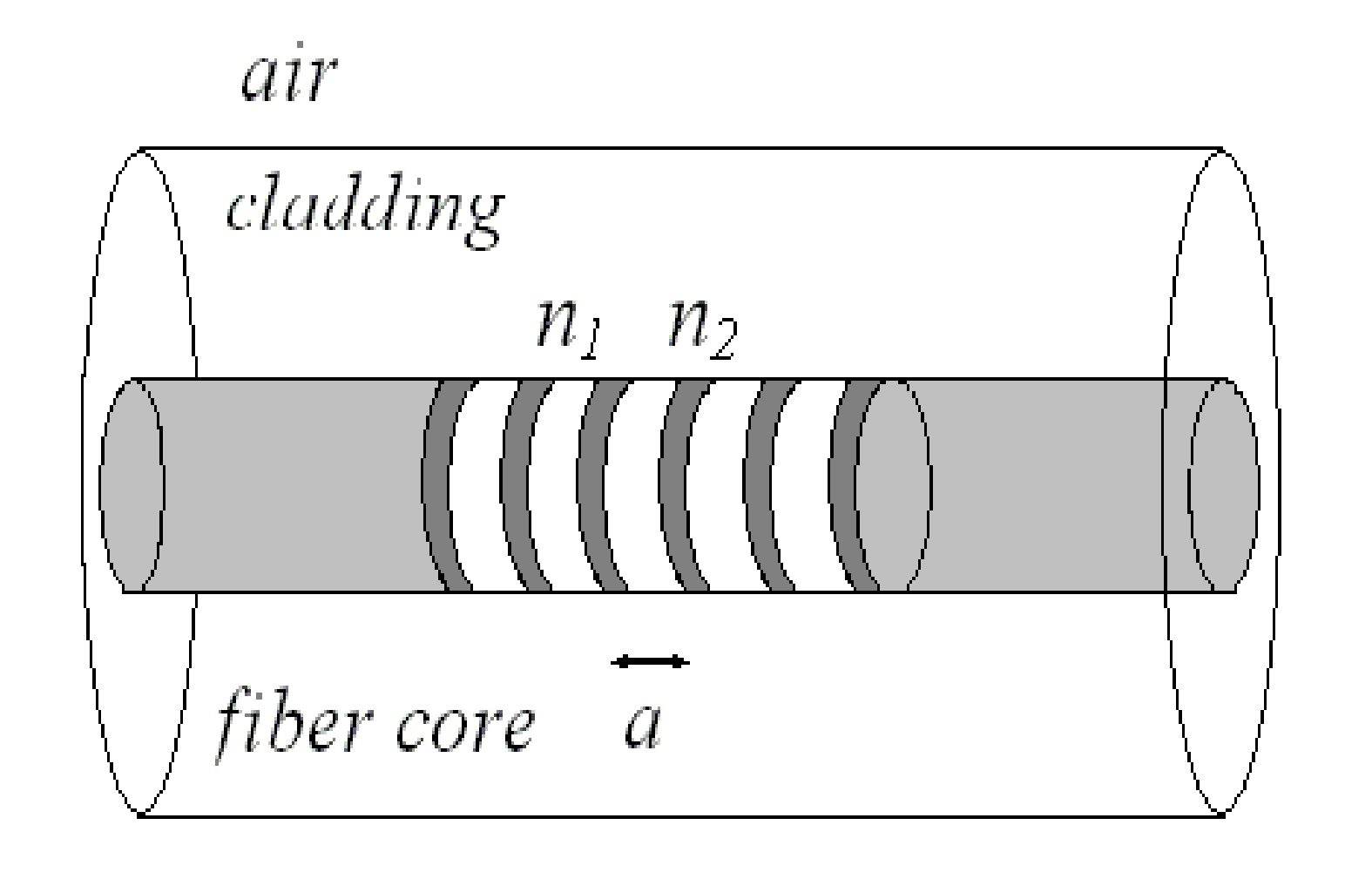
Figure 1: A fiber Bragg grating with an uniform periodic modulation of the index of refraction.

In our numerical calculations the FBG consists of 40000 Si layers of length 158.8 nm and index of refraction 3.48 alternating with 39999 air layers of 553.2 nm wide. The grating period is then 712.0 nm and the total size of our arrangement 28.5 mm. This corresponds to a realistic structure used in slow light experiments POV05 ; MOK06 , but the results are of general validity.

To obtain the transmission coefficient of the previous structure $|t_{N}|^{2}$, we employ the characteristic determinant method AG91 . This formalism allows one to express the transmission coefficient of a wave propagating in a 1D periodic structure through the determinant $D_{N}$, which depends on the amplitudes of transmission and reflection of a single cell. Via this determinant method, the inverse of the transmission coefficient $|t_{N}|^{-2}$ for this structure can be written as CU96

$$|t_{N}|^{-2}=1+\left[{\frac{k_{1}^{2}-k_{2}^{2}}{2k_{1}k_{2}}}\sin(k_{2}L_{2})\right]^{2}\frac{\sin^{2}(N\beta a/2)}{\sin^{2}(\beta a)},$$ (5)

where $N-1$ is the total number of layers and $\beta$ plays the role of quasimomentum of the system, and is defined by

$$\cos(\beta a)=\cos(k_{1}L_{1})\cos(k_{2}L_{2})-\left({\frac{k_{1}^{2}+k_{2}^{2}}{2k_{1}k_{2}}}\right)\sin(k_{1}L_{1})\sin(k_{2}L_{2}).$$ (6)

When the modulus of the RHS of Eq. (6) is greater than 1, $\beta$ has to be taken as imaginary. This situation corresponds to a forbidden frequency window.

In Fig. 2(a) we have represented the transmission coefficient of our grating $|t_{N}|^{2}$ as a function of the frequency $\omega$ for $N=10$ to illustrate its behavior. The realistic grating corresponds to Fig. 2(b) where $N=80000$ (with 28.5 mm length). There are so many peaks that they appear as a black region in the figure, and they cannot be resolved in the scale shown.

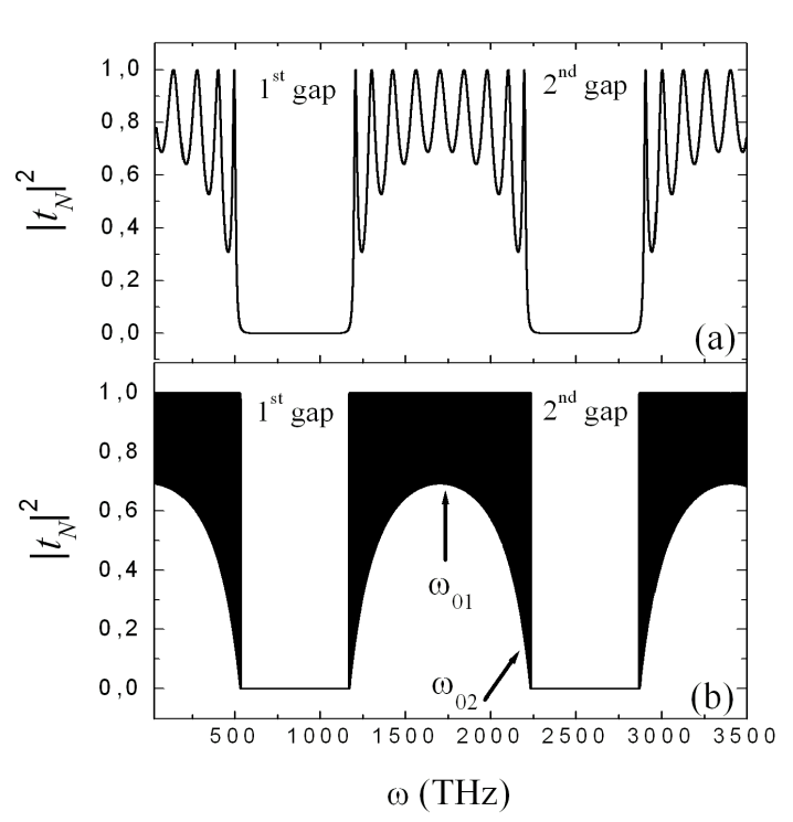
Figure 2: Transmission coefficient $|t_{N}|^{2}$ as a function of the frequency $\omega$ for (a) $N=10$ and (b) $N=80000$. The regions around the frequencies $\omega_{01}=1754$ THz and $\omega_{02}=2225$ THz marked with arrows are expanded in Fig. 3.

In order to study $|t_{N}|^{2}$ in detail as a function of the position in the frequency transmission window we plot on a much larger scale a region near the center, Fig. 3(a), and a region near the edge, Fig. 3(b). The center of these two regions, $\omega_{01}=1754$ THz and $\omega_{02}=2225$ THz, are marked with arrows in Fig. 2(b) and they correspond to wavelengths within the infrared spectrum ($\lambda_{01}=1073.6$ nm and $\lambda_{02}=846.3$ nm) for the second transmission window. In percentage terms, the frequencies $\omega_{01}$ and $\omega_{02}$ are at 45 % and 1 % of the total window width from the upper frequency window edge, respectively. Similar results will be obtained for the other frequency windows.

The dashed lines in Fig. 3(a) and 3(b) correspond to Lorentzian fits of the central resonance for each case. We note that the Lorentzian curves fit fairly well the peaks in the transmission coefficients in all cases studied. We can in fact justify this by having a close look into Eq. (5) where the term $|t_{N}|^{-2}-1$ is the product of a highly oscillating function, $\sin^{2}(N\beta a/2)$, and factors independent of the number of layers and which vary very slowly on the scale of one peak. The oscillating function can be approximated around each of its minimum by a quadratic term, resulting in a Lorentzian curve for the transmission coefficient. We will use this expansion later on to calculate the width of each peak.

One observes that the resonances are narrower and closer to each other near the transmission window edge. From now on, we will denote by $\Gamma_{\rm r}$ the energy width of each individual Lorentzian resonance and by $\Delta\omega_{\rm r}$ the frequency separation between two consecutive resonances. The ratio $\Gamma_{\rm r}/\hbar\Delta\omega_{\rm r}$, which we will see that constitutes an important parameter of the problem, decreases as we approach the window edge. For this reason, the overlap between Lorentzians and the transmission in the midpoint between peaks is very small in this region.

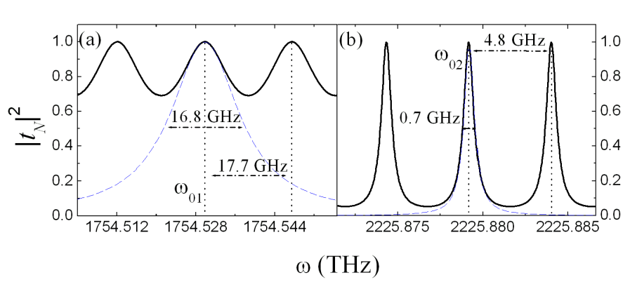
Figure 3: Transmission coefficient $|t_{N}|^{2}$ versus $\omega$ for a region near the center (a) and the edge (b) of the transmission window plotted in Fig. 2(b). The dashed curves are Lorentzian fits for a single peak.

We can now obtain analytical expressions for the width $\Gamma_{\rm r}$ and the separation $\Delta\omega_{\rm r}$. The term within brackets in Eq. (5) only depends on the properties of one layer, while the quotient of the sine functions contains information about the interference between different layers. The transmission coefficient $|t_{N}|^{2}$ is equal to 1 when $\sin{(N\beta a/2)}=0$ and $\beta$ is different from 0. This condition occurs for

$$\beta a=\frac{2\pi n}{N}\qquad n=1,\dots,N/2-1,$$ (7)

and it corresponds to a resonant frequency. Considering that each resonance is a Lorentzian function centered about the resonant frequency $\omega_{\rm r}$ with full width $\Gamma_{\rm r}/\hbar$, we can write the inverse of the transmission coefficient for one resonance as

$$|t|^{-2}=1+\frac{4\hbar^{2}}{\Gamma_{\rm r}^{2}}(\omega-\omega_{\rm r})^{2}.$$ (8)

Expanding the sine in the numerator of Eq. (5) near a resonance we have

$$\sin^{2}\left(\frac{N\beta a}{2}\right)\simeq\frac{N^{2}(\delta\beta)^{2}a^{2}}{4}\simeq\frac{N^{2}a^{2}}{4v_{\rm g}^{2}}(\delta\omega)^{2},$$ (9)

so, Eq. (5) can be rewritten as

$$|t_{N}|^{-2}=1+\left[\frac{(k_{1}^{2}-k_{2}^{2})\sin(k_{2}L_{2})}{2k_{1}k_{2}\sin(\beta a)}\right]^{2}\frac{N^{2}a^{2}}{4v_{\rm g}^{2}}(\delta\omega)^{2},$$ (10)

where we have taken into account the definition of the group velocity $v_{\rm g}$ in terms of the quasimomentum $\beta$

$$v_{\rm g}=\frac{\delta\omega}{\delta\beta}.$$ (11)

We can derive an expression for the frequency distance between two consecutive resonances $\Delta\omega_{\rm r}$ by taking finite differences in Eq. (7) (resonance condition)

$$\Delta\omega_{\rm r}=v_{\rm g}\Delta\beta=v_{\rm g}\frac{2\pi}{Na},$$ (12)

and after comparing Eqs. (8) and (10) we can identify

$$\frac{\Gamma_{\rm r}}{\hbar\Delta\omega_{\rm r}}=\left(\frac{2|\sin(\beta a)|}{\pi}\right)\left[{\frac{k_{1}^{2}-k_{2}^{2}}{2k_{1}k_{2}}}\sin(k_{2}L_{2})\right]^{-1}.$$ (13)

As we will see, the ratio $\Gamma_{\rm r}/\hbar\Delta\omega_{\rm r}$ is a very significant parameter which is independent of the number of layers of our grating. In Fig. 4 we plot this ratio, calculated via Eq. (13), as a function of the frequency $\omega$ (left axis, squares for $N=10$ and solid line for $N=80000$). One observes that in the center of the transmission windows the ratio $\Gamma_{\rm r}/\hbar\Delta\omega_{\rm r}$ reaches its maximum, which is roughly 1.0 in our case. This ratio also tends to zero as we approach the optical mirror region, what has important consequences on the distortion of the transmitted pulses, as we will see.

It is well known that the group velocity tends to zero when approaching the edge of the transmission windows. This is the reason why most authors have tried to work in this region to slow down light as much as possible. In Fig. 4 we also show the ratio of the group velocity to the speed of light in vacuum $v_{\rm g}/c$ (right axis, dashed line) versus the frequency $\omega$. As expected, this ratio tends to zero as we approach the transmission window edge.

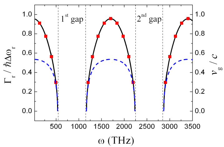
Figure 4: The ratio $\Gamma_{\rm r}/\hbar\Delta\omega_{\rm r}$ (left axis, squares for $N=10$ and solid line for $N=80000$) and the fractional group velocity $v_{\rm g}/c$ (right axis, dashed line) versus the frequency $\omega$.

III Pulse propagation through the transmission window

Let us now study how an incident gaussian pulse $\Psi_{\rm inc}(t)$ traverses our 1D grating depending on the position of its central frequency in the transmission window. We will consider the two frequencies described in Fig. 2(b), $\omega_{01}=1754$ THz (near the center) and $\omega_{02}=2225$ THz (near the edge). In both cases, we have chosen a pulse width of 68.4 ps which corresponds to a bandwidth of about 41.3 GHz.

For these broadband pulses we can approximate the transmission amplitude of our grating by a periodic function of $\omega$ that can be written as the sum of a given function displaced periodically by a fixed amount

$$t_{N}(\omega)=\sum_{n}f(\omega-\Delta\omega_{\rm r}n,\Gamma_{\rm r}).$$ (14)

As before, $\Delta\omega_{\rm r}$ is the frequency separation between consecutive resonances. As we saw in the previous section, we can consider, to a very good approximation, $f$ to be a Lorentzian function of width $\Gamma_{\rm r}$. Under these conditions, we have shown in the Appendix that the transmitted pulse consists of an exponentially decreasing series of similar pulses given by

$$\Psi_{\rm tr}(t)=\frac{\sqrt{2\pi}C}{\Delta\omega_{\rm r}}\ \exp\left[-\frac{\Gamma_{\rm r}|t|}{2\hbar}\right]\ \sum_{n}\Psi_{\rm inc}\left(t-\frac{2\pi n}{\Delta\omega_{\rm r}}\right),$$ (15)

where $C$ is a normalization constant. If we neglect overlap between consecutive peaks, it is easy to deduce from the previous expression that the ratio $r$ between the intensity of two of these peaks is equal to

$$r=\exp\left[-\frac{2\pi\Gamma_{\rm r}}{\hbar\Delta\omega_{\rm r}}\right].$$ (16)

According to this result, Eq. (16), Fig. 4 which represents $\Gamma_{\rm r}/\hbar\Delta\omega_{\rm r}$ also corresponds to the frequency dependence of the factor $r$ on a logarithmic scale.

Near $\omega_{01}$ the ratio $r$ is very small (about a $0.25\%$) and the secondary peak cannot be appreciated in the main part of Fig. 5(a). In the inset we show the same data on a large vertical scale, in order to appreciate more clearly this secondary peak, whose temporal separation with the principal peak is about 355.36 ps. Near $\omega_{02}$ the parameter $\Gamma_{\rm r}/\hbar\Delta\omega_{\rm r}$ is lower than in the previous case and the ratio $r$ is greater (roughly 40 %) and several peaks can be appreciated, as in Fig. 5(b). It is clear that near the transmission window edge the importance of secondary peaks is significant. Their separation, 1297.80 ps, is larger than in the center of the window because this is inversely proportional to the frequency distance between two consecutive Lorentzian resonances $\Delta\omega_{\rm r}$ (see Eq. (15)).

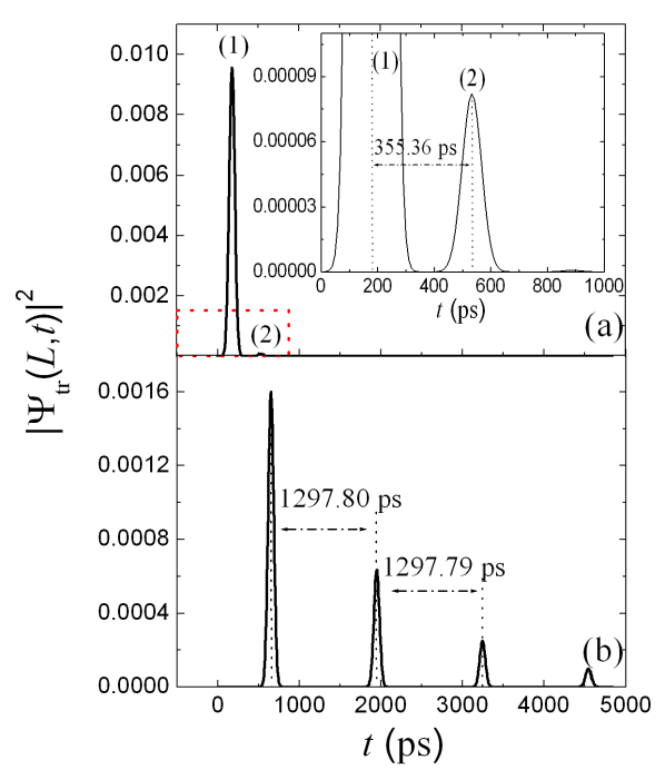
Figure 5: Transmitted pulses through our 1D grating for an incident gaussian pulse of width 68.4 ps and a central frequency equal to $\omega_{01}=1754$ THz (a) and $\omega_{02}=2225$ THz (b). The inset in (a) corresponds to the same curve as in the main part with a different vertical scale.

In view of the previous results, for the high contrasts considered, it is convenient to use pulses with its central frequency near the center of the transmission window (so as to reduce as much as possible the ratio between consecutive peaks), despite the fact that the group velocity $v_{\rm g}$ is higher in this region. In Fig. 6 we compare the shape of a free pulse of width 6.84 ps (dashed line) with its corresponding transmitted pulse (solid line). The central frequency of the incident pulse is $\omega_{01}=1754$ THz. This is an ultrashort temporal pulse (bandwidth of 413 GHz) desirable for telecommunication systems MORK05 ; SED07 . We can observe a large delay of 12 pulses without significant pulse broadening and high transmission. We will return to this point in the next section.

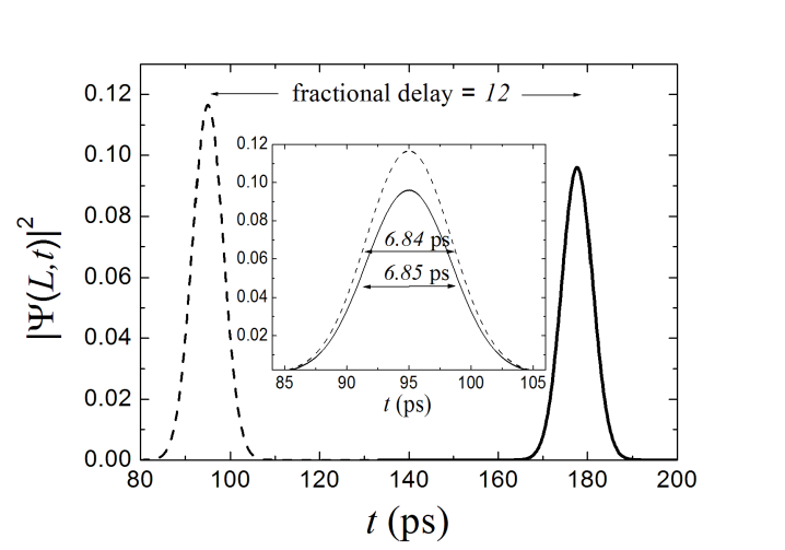
Figure 6: Free propagation pulse of width 6.84 ps (dashed line) and its corresponding transmitted pulse (solid line) for a central frequency of $\omega_{01}=1754$ THz which traverses the 1D grating described in Fig. 1.

IV Bandwidth dependence of the transmitted pulse parameters

Let us now study numerically how significant pulse parameters, such as its transmission coefficient and its fractional delay, depend on the frequency bandwidth of the incident pulse $2\Delta\omega$.

In Fig. 7(a) we represent the transmission coefficient $|t_{N}|^{2}$ as a function of $2\Delta\omega$ for an incident pulse whose central frequency is $\omega_{01}=1754$ THz. The left dashed line corresponds to the frequency width of the Lorentzian resonance which is equal to 16.8 GHz (see Fig. 3(a)) while the right dashed line (approximately 34 GHz) is the lower value of $2\Delta\omega$ for which the transmission coefficient $|t_{N}|^{2}$ is independent of the frequency bandwidth. One observes that for short bandwidths the transmission coefficient is practically unity because the frequency pulse is narrower enough to lay within a transmission resonance. As we increase the bandwidth $2\Delta\omega$ the frequency pulse extends over several resonances what results in a lower transmission coefficient. When the number of resonances within the frequency pulse is large enough, the transmission coefficient $|t_{N}|^{2}$ reaches a constant value independent of the frequency bandwidth, in this case 0.86. This is the regime where the traversal time is well approximated by the classical expression, Eq. (4). For values of $2\Delta\omega$ greater than 34 GHz the transmitted pulse consists of a serie of decreasing pulses as described in the previous section (see Fig. 5(a)) with a short ratio $r=0.25\%$.

Similar comments can be applied to Fig. 7(b) where the central frequency of the incident pulse is now equal to $\omega_{02}=2225$ THz. The frequency width of the Lorentzian resonance (left dashed line) is 0.7 GHz (see Fig. 3(b)) while the bandwidth limit (right dashed line) is approximately 6.6 GHz. One observes that the transmission coefficient $|t_{N}|^{2}$ reaches a lower value than in the previous case. The reason is that, as explained in Sec. II, the overlap between Lorentzians is negligible near the edge and the transmission in the midpoint between peaks reduces considerably.

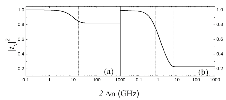
Figure 7: Transmission coefficient $|t_{N}|^{2}$ as a function of the bandwidth $2\Delta\omega$ for an incident pulse whose central frequency is $\omega_{01}=1754$ THz (a) and $\omega_{02}=2225$ THz (b). In both figures, the left dashed line corresponds to the frequency width of each Lorentzian resonance and the right dashed line is the lower value of $2\Delta\omega$ for which the transmission coefficient $|t_{N}|^{2}$ is independent of the frequency bandwidth.

As regard the fractional delay, we show in Fig. 8 this parameter versus $2\Delta\omega$ for $\omega_{01}$ (continuous line) and $\omega_{02}$ (dashed line). We have performed these calculations via Eq. (3) though similar results can be obtained with a classical treatment, Eq. (4). It can be appreciated that the fractional delay is, as expected, greater for values of $\omega_{0}$ near the frequency window edge (where the group velocity is lower). However the distortion of the transmitted pulse, which is related to the factor $r$, is considerably high in this region (see Fig. 5(b)).

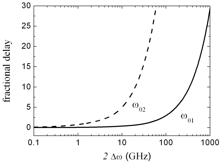
Figure 8: Fractional delay versus the frequency bandwidth of the incident pulse $2\Delta\omega$ for two different values of the central frequency, $\omega_{01}$ (continuous line) and $\omega_{02}$ (dashed line). In the latter case, the ratio $r$ is quite large.

In view of the previous results one can conclude that the distortion of the transmitted pulse is unacceptable large when its central frequency lays near the edge of the transmission window. So, it is convenient to work near the center of this frequency window, even though it corresponds to larger group velocities.

V Discussion and Conclusions

We have analyzed the transmission properties of pulses through one-dimensional periodic structures with alternating index of refraction $n_{1}$ and $n_{2}$. We also explored the best conditions to achieve the maximum delay with the minimum possible pulse distortion.

As we have already mentioned, in the present work we have not included either absorption or layer variability. We think that this is well justified for most situations of interest. In a typical device employed in slow light experiments, the losses due to absorption are negligible up to distances of the order of 2 m MOK06 . As the structures considered here are 3cm long, we do not expect any significant effect due to absorption. As regard of layer variability, it is more difficult to estimate its effects, but the following argument convinced us that they again do not need to be considered in first instance. MacGurn et al. McCh93 studied the localization length associated with layer variability and concluded that its value decreases (and the importance of its effects increases) as we approach the band edge. They performed a numerical simulation for a layer width variability of 20 % and obtained a localization length of roughly 20 times the layer period. Lhommé et al. LC05 estimated that the typical layer width variability in the type of devices considered by us to be about $0.2$ %. As in one-dimensional systems the localization length depends on the inverse of the square of the disorder, we estimate that the minimum localization length will be approximately $2\cdot 10^{5}$ layer spacings. The devices considered have 40000 periods and so we expect a negligible decrease of the pulse amplitude due to localization by disorder. Near the band edge localization effects are potentially more important, due to shorter localization lengths, so one should be careful with large layer variability in this region.

For our ideal model, the transmission coefficient $t_{N}$ can be well approximated by a sum of Lorentzian resonances and the ratio between their width $\Gamma_{\rm r}$ and their separation $\Delta\omega_{\rm r}$ is a significant parameter to characterize the distortion of the transmitted pulse, which consists of an exponentially decreasing series of similar pulses given by Eq. (15). This pulse distortion is greater near the edge of the transmission window, so it is convenient to work with pulse frequencies near the center of this window. Our numerical calculations show fractional delays of 12 pulse widths, without significant distortion and high transmission, for 6.84 ps width gaussian pulses.

Appendix A Transmitted pulse through a periodic arrangement of Lorentzian resonances

Let us consider that the transmission amplitude of our structure $t_{N}(\omega)$ is a periodic function in $\omega$ as given by Eq. (14). The transmitted wavefunction $\Psi_{\rm tr}(t)$ will then be given by

$$\Psi_{\rm tr}(t)=C\ \int_{-\infty}^{+\infty}d\omega\exp[-i\omega t]\ \Phi_{\rm inc}(\omega)\sum_{n}f(\omega-\Delta\omega_{\rm r}n,\Gamma_{\rm r}),$$ (17)

where $C$ is a normalization constant. After introducing the parameter $v\equiv\omega-\Delta\omega_{\rm r}n$ and performing some trivial calculations one can write Eq. (17) as

$$\Psi_{\rm tr}(t)=C\ \sum_{n}\exp[-i\Delta\omega_{\rm r}nt]\int_{-\infty}^{+\infty}dvf(v,\Gamma_{\rm r})\Phi_{\rm inc}(v+\Delta\omega_{\rm r}n)\exp[-ivt].$$ (18)

For a large pulse over the frequency domain, the wavefunction $\Phi_{\rm inc}(\omega)$ is practically constant (so we can extract this term out of the integral in the previous equation). We can also express the first exponential in Eq. (18) as an integral of the delta function and obtain

$$\Psi_{\rm tr}(t) = C\ \sum_{n}\left[\left(\int_{-\infty}^{+\infty}d\omega\ \delta(\omega-\Delta\omega_{\rm r}n)\exp[-i\omega t]\ \Phi_{\rm inc}(\omega)\right)\right.$$ (19)

$$\times \left.\left(\int_{-\infty}^{+\infty}dvf(v,\Gamma_{\rm r})\exp[-ivt]\right)\right].$$

Taking into account the expression for the Fourier series of a Dirac comb

$$\sum_{n}\delta(\omega-\Delta\omega_{\rm r}n)=\frac{1}{\Delta\omega_{\rm r}}\sum_{n}\exp\left[2\pi i\omega\frac{n}{\Delta\omega_{\rm r}}\right],$$ (20)

and performing the inverse Fourier transform of the Lorentzian $f(v,\Gamma_{\rm r})$

$$\int_{-\infty}^{+\infty}dvf(v,\Gamma_{\rm r})\exp[-ivt]=\sqrt{2\pi}\ \exp\left[-\frac{\Gamma_{\rm r}|t|}{2\hbar}\right],$$ (21)

we have for the transmitted wavefunction

$$\Psi_{\rm tr}(t)=\frac{\sqrt{2\pi}C}{\Delta\omega_{\rm r}}\ \exp\left[-\frac{\Gamma_{\rm r}|t|}{2\hbar}\right]\ \sum_{n}\left[\int_{-\infty}^{+\infty}d\omega\exp\left[i\omega\left(\frac{2\pi n}{\Delta\omega_{\rm r}}-t\right)\right]\Phi_{\rm inc}(\omega)\right].$$ (22)

Identifying the term within brackets in Eq. (22) as the inverse Fourier transform of the incident wavefunction $\Psi_{\rm inc}(t-2\pi n/\Delta\omega_{\rm r})$ multiplied by $2\pi$, we can finally derive the expression for $\Psi_{\rm tr}(t)$, Eq. (15).

One observes that the transmitted wavefunction $\Psi_{\rm tr}(t)$ is formed by a series of equally spaced peaks, separated by the inverse of $\Delta\omega_{\rm r}$, and modulated by an exponentially decaying factor $\exp[-\Gamma_{\rm r}|t|/2\hbar]$. The ratio between the intensity of two consecutive peaks $r$ is then given by Eq. (16).

References

- (1) L. V. Hau, S. F. Harris, Z. Dutton and C. H. Behroozi, Nature 397, 594 (1999).
- (2) C. Liu, Z. Dutton, C. H. Behroozi and L. V. Hau, Nature 409, 490 (2001).
- (3) D. F. Philips, A. Fleischhauer, A. Mair, R. L. Walsworth and M. D. Lukin, Phys. Rev. Lett. 86, 783 (2001).
- (4) Y. Okawachi et al., Phys. Rev. Lett. 94, 153902 (2005).
- (5) K. Y. Song, M. G. Herráez and L. Thévenaz, Opt. Express 13, 82 (2005).
- (6) M. L. Povinelli, S. G. Johnson and J. D. Joannopoulos, Opt. Express 13, 7145 (2005).
- (7) M. Notomi et al., Phys. Rev. Lett. 87, 253902 (2001).
- (8) H. Gersen et al., Phys. Rev. Lett. 94, 073903 (2005).
- (9) D. Mori and T. Baba, Appl. Phys. Lett. 85, 1101 (2004).
- (10) Y. A. Vlasov, M. O’Boyle, H. F. Hamann and S. J. McNab, Nature 438, 65 (2005).
- (11) J. T. Mok, C. M. de Sterke, I. C. M. Littler and B. J. Eggleton, Nature Phys. 2, 775 (2006).
- (12) S. Sarkar, Y. Guo and H. Wang, Opt. Express 14, 2845 (2006).
- (13) I. Novikova, D. F. Phillips and R. L. Walsworth, Phys. Rev. Lett. 99, 173604 (2007).
- (14) R. W. Boyd, D. J. Gauthier, A. L. Gaeta and A. E. Willner, Phys. Rev. A 71, 023801 (2005).
- (15) O. del Barco, M. Ortuño and V. Gasparian, Phys. Rev. A 74, 032104 (2006).
- (16) V. Gasparian, M. Ortuño, J. Ruiz and E. Cuevas, Phys. Rev. Lett. 75, 2312 (1995).
- (17) A. G. Aronov, V. Gasparian and U. Gummich, J. Phys.: Condens. Matter 3, 3023 (1991).
- (18) V. Gasparian, M. Ortuño, J. Ruiz, E. Cuevas and M. Pollak, Phys. Rev. B 51, 6743 (1995).
- (19) E. Cuevas, V. Gasparian, M. Ortuño and J. Ruiz, Z. Phys. B 100, 595 (1996).
- (20) J. Mørk, R. Kjaer, M. van der Poel and K. Yvind, Opt. Express 13, 8136 (2005).
- (21) F. G. Sedgwick et al., Opt. Express 15, 747 (2007).
- (22) A. R. McGurn et al., Phys. Rev. B 47, 13120 (1993).
- (23) F. Lhommé et al., Appl. Opt. 44, 493 (2005).