New Geometric Representations of the CMB 2pcf

Abstract

When searching for deviations of statistical isotropy in CMB, a popular strategy is to write the two-point correlation function (2pcf) as the most general function of four spherical angles (i.e., two unit vectors) in the celestial sphere. Then, using a basis of bipolar spherical harmonics, statistical anisotropy will show up if and only if any coefficient of the expansion with non-trivial bipolar momentum is detected – although this detection will not in general elucidate the origin of the anisotropy. In this work we show that two new sets of four angles and basis functions exist which completely specifies the 2pcf, while, at the same time, offering a possible geometrical interpretation of the mechanisms generating the signal. Since the coefficients of these expansions are zero if and only if isotropy holds, they act as a simple and geometrically motivated null test of statistical isotropy, with the advantage of allowing cosmic variance to be controlled in a systematic way. We report the results of the application of these null tests to the latest temperature data released by the Planck collaboration.

I Introduction

Given the unprecedented limits on cosmological parameters achieved with Planck data releases Ade2014d ; Ade2015a , an important follow-up question is whether the same data contain traces of physics beyond the standard $\Lambda$CDM model. While deep field surveys Laureijs2011 ; Abate2012 ; Benitez2014 aim to unveil the specific nature of dark matter and dark energy, and thus of the energy content of our universe, CMB observations are special in the sense that they provide a unique window to both the physics of the early inflationary universe and of its global shape, i.e., its geometry and topology Cornish2004 ; Kunz2006 ; Ade2015 ; Fabre:2013wia .

From the statistical point of view, finding evidences of new features of inflationary physics or of the shape of the universe usually translates into cosmological detections of non-Gaussianity and statistical anisotropy, respectively (but not necessarily Schmidt:2012ky ). As it turns out, however, observational bounds from CMB on non-Gaussianity Komatsu2003 ; Ade2014c ; Ade2015b did not allow us to discriminate inflationary models, and the hope now lies on the possibility that future measurements of polarization $B$-modes of CMB Bouchet2011 will better elucidate the physics of the early universe. The physics describing the global topology and geometry of the universe, on the other hand, is not only much less constrained by CMB Ade2015 , but is also equally fundamental to the beyond-$\Lambda$CDM program. In this regard, the existence of statistical anomalies at the largest CMB angles (see Ref. Copi2010 for a comprehensive review) can be optimistically seen as an indication of spatial anisotropy at the horizon scales Pitrou2008 , although the conservative minded would also remind us of possible unaccounted systematic effects Hanson2010a , or even the less exciting case of statistical flukes Bennett2011 .

Regardless of the final words on CMB anomalies, however, one is rightfully justified to question the validity of the statistically isotropic scenario, given its deep connections with the symmetry hypothesis about our universe. Thus motivated, this paper addresses the question of how to constrain deviations from statistical isotropy in a geometrically meaningful and model-independent way.

The general recipe for describing the statistics of a Gaussian and statistically isotropic CMB map is straightforward. Assuming that the geometry of the universe is everywhere rotationally invariant, all we need to do is to compute the correlation between the temperature fluctuations $\Delta T$ at directions $\hat{n}$ and $\hat{n}^{\prime}$, given by

$$C(\hat{n},\hat{n}^{\prime})=\left.\left\langle\Delta T(\hat{n})\Delta T(\hat{n}^{\prime})\right\rangle\right|_{\cos\theta=\hat{n}\cdot\hat{n}^{\prime}}\equiv C(\theta)\,.$$ (1)

However, if there are departures from statistical isotropy, either of systematic Hanson2010a , astrophysical Yoho01072013 ; Ade2014b ; Amendola2011 or cosmological Pitrou2008 ; Kahniashvili2008a ; BH08 ; Durrer1998 origin, the two-point correlation function (2pcf) will depend on other angles relating $\hat{n}$ and $\hat{n}^{\prime}$; in this case, $C(\theta)$ no longer exhausts the statistics of the universe. Thus, if we want to go beyond the $\Lambda$CDM framework, the central question is how to parameterize deviations from Eq. (1) in a meaningful, and hopefully practical, way.

The angular correlation function has come under considerable scrutiny. It was first noticed by the COBE-DMR team Hinshaw:1996ut that $C(\theta)$ was unexpectedly close to zero for $\theta\gtrsim 60^{\circ}$. This lack of correlations was confirmed by the Wilkinson Microwave Anisotropy Probe (WMAP) team in their analysis of their first year of data Spergel2003 . Though WMAP claimed to have greatly reduced significance in future releases, Copi et al. showed Copi:2006tu that in fact this absence of large-angle correlations persisted on the sky outside the galaxy in the third year release, and in all subsequent releases, including the first-year Planck release Copi:2008hw ; Copi:2010na ; Copi:2013cya . Those findings have since been confirmed by others Hajian:2007pi ; Bunn:2008zd , although no satisfactory explanation exists. It has been suggested Copi:2013zja ; Yoho:2013tta ; Yoho:2015bla that one might be able to test whether the anomalous vanishing of the temperature-temperature correlation function is due to new physics or just a statistical anomaly by examining other two-point correlation functions (eg. the $E$-mode-$E$-mode correlation function) on similarly large angles.

A common strategy for parameterizing deviations of isotropy in the CMB is to use a complete set of basis functions to perform a multipolar expansion of the 2pcf. Since the latter is defined by the product of two functions on the CMB sphere, we could simply use the product of two independent spherical harmonics as such basis. Instead, it has become a standard practice to use a basis of total angular momentum eigenfunctions, also known as bipolar spherical harmonics Varshalovich1988a , to do the expansion. Besides sharing most of the mathematical properties of the standard spherical harmonics, the advantage of the bipolar harmonics is that they encode deviations of isotropy in the total angular momentum of the coefficients of the expansion. Thus, any measurement of a multipolar coefficient with a non-trivial total angular momentum eigenvalue is an indication of statistical anisotropy. This program was introduced by Hajian and Souradeep Hajian2003a ; Hajian2004 ; Hajian2005 , and has been fruitfully applied to CMB since then Joshi2010 ; Ade2014b ; Book2012 ; Kamionkowski2011 ; Hajian2006 .

Since the bipolar spherical harmonics form a basis for square-integrable functions on the Hilbert space where the 2pcf is defined, they offer a very general framework for studying the statistics of the CMB. However, it has some limitations, too. First, the multipolar coefficients of the bipolar expansion, while serving as a null indicator of anisotropy, do not provide a physical interpretation of the underlying signal straightforwardly, and for that one has to resort to other tools Kumar2014 . Second, in a more symmetric situation – whether real or expected – it is not clear how the degrees of freedom of the bipolar spherical harmonics could be combined to reduce cosmic variance.

This paper is based on the idea that, given two unit vectors rooted at the origin of the CMB sphere, two new and unique geometrical objects can be formed: a great circle and (the boundary circle of) a spherical cap – or, if we include the interior of the sphere, a disc and a cone. Using the set of angles defined by these objects, one can introduce a complete set of basis functions that characterize the 2pcf, and whose multipolar coefficients offer a direct and geometrically motivated null test of statistical isotropy. Moreover, since the angles used to represent the 2pcf have a clear geometrical interpretation, it may at times be physically well-motivated to integrate, average or marginalize over one of them.

This work is organized as follows. After reviewing the basics of the bipolar spherical harmonic formalism in Sec. II.1, we introduce the new geometric representations of the 2pcf in Secs. II.2 and II.3, where we also show how they recover the usual 2pcf in the isotropic limit. In Sec. III we show how these new functions can be used to construct null geometrical tests of statistical isotropy. Finally, we present the results of null tests applied to the latest temperature maps released by the Planck team in Sec. III.1. We conclude in Sec. IV with some perspectives of future developments.

II Geometric Representations

We start by recalling the basic definitions and notations used in CMB statistics. The temperature fluctuation field is a real function on the sphere, and can thus be expanded as

$$\Delta T(\hat{n})=\sum_{l,m}a_{lm}Y_{lm}(\hat{n})\,,$$

where $\hat{n}=(\theta,\phi)$. In the canonical $\Lambda$CDM cosmological model, the $a_{lm}$ are realizations of a Gaussian-random and statistically independent variables. In this case the expectation value of the two-point correlation function is

$$C\left(\hat{n}_{1},\hat{n}_{2}\right)=\!\!\sum_{\begin{subarray}{c}l_{1},m_{1}\\ l_{2},m_{2}\end{subarray}}\!\!\left\langle a_{l_{1}m_{1}}a^{*}_{l_{2}m_{2}}\right\rangle Y_{l_{1}m_{1}}(\hat{n}_{1})Y^{*}_{l_{2}m_{2}}(\hat{n}_{2})\,.$$ (2)

The set of coefficients $\left\langle a_{l_{1}m_{1}}a^{*}_{l_{2}m_{2}}\right\rangle$ form the covariance matrix, and in the canonical statistically isotropic case

$$\left\langle a_{l_{1}m_{1}}a_{l_{2}m_{2}}^{*}\right\rangle=C_{l_{1}}\delta_{l_{1}l_{2}}\delta_{m_{1}m_{2}}\,.$$ (3)

Any non-zero off-diagonal term in the covariance matrix is a measure of statistical anisotropy.

The 2pcf is symmetric by definition

$$C(\hat{n}_{1},\hat{n}_{2})=C(\hat{n}_{2},\hat{n}_{1})\,.$$ (4)

As we shall see, this symmetry imposes restrictions on the eigenvalues of the eigenfunctions (and consequently on the multipolar coefficients) that we introduce below.

II.1 Bipolar representation

A convenient basis for expanding the 2pcf is given by the bipolar spherical harmonics Varshalovich1988a , which are defined as the tensor product of two spherical harmonics

$${\cal Y}_{LM}^{l_{1}l_{2}}(\hat{n}_{1},\hat{n}_{2})\equiv\left[\vec{Y}_{l_{1}}(\hat{n}_{1})\otimes\vec{Y}_{l_{1}}(\hat{n}_{2})\right]_{LM}\,,$$

where $\vec{Y}_{l_{1}}$ is a shorthand notation for $(Y_{l_{1},-l_{1}};\dots;Y_{l_{1},+l_{1}})$. In terms of this basis the 2pcf reads

$$C\left(\hat{n}_{1},\hat{n}_{2}\right)=\sum_{L,M}\sum_{l_{1},l_{2}}{\cal A}_{l_{1}l_{2}}^{LM}{\cal Y}_{LM}^{l_{1}l_{2}}(\hat{n}_{1},\hat{n}_{2})\,.$$ (5)

The coefficients ${\cal A}_{l_{1}l_{2}}^{LM}$ are called the BipoSH spectrum Hajian2003a ; Hajian2004 ; Hajian2005 . They are given by a quadratic combination of the $a_{lm}$:

$${\cal A}_{l_{1}l_{2}}^{LM}=\sum_{m_{1},m_{2}}C_{l_{1}m_{1}l_{2}m_{2}}^{LM}\left\langle a_{l_{1}m_{1}}a_{l_{2}m_{2}}\right\rangle\,,$$ (6)

where $C_{l_{1}m_{1}l_{2}m_{2}}^{LM}$ are the Clebsch-Gordan coefficients. In the case (3) of statistical isotropy they reduce to

$${\cal A}_{l_{1}l_{2}}^{LM}=(-1)^{l_{1}}\sqrt{2l_{1}+1}\,C_{l_{1}}\,\delta_{l_{1}l_{2}}\delta_{L0}\delta_{M0}\,,$$

so that any statistically significant detection of a non-zero ${\cal A}_{l_{1}l_{2}}^{LM}$ with $L>0$ is a sign of statistical anisotropy. This property makes the BipoSH coefficients a very convenient null test for statistical anisotropy.

II.2 Anisotropies through conic modulations

Given two unit vectors, $\hat{n}_{1}=(\chi_{1},\phi_{1})$ and $\hat{n}_{2}=(\chi_{2},\phi_{2})$, rooted at the origin, they define a cone on the unit sphere, obtained by rotating those vectors about an axis collinear to $\hat{n}_{12}\propto{\hat{n}_{1}+\hat{n}_{2}}$. Each cone can be completely described by three angles: the opening angle $\chi$ of the cone, and two angles $\Theta$ and $\Phi$ giving the orientation of the axis $\hat{n}_{12}$. The ordered pair of directions, $(\hat{n}_{1},\hat{n}_{2})$, is fixed by a fourth angle $\eta$ specifying their position on the circle bounding the intersection of the cone with the unit sphere – see Fig. 1.

Figure 1: Two unit vectors in the CMB sphere will always define cones. The number of angles characterizing a given cone is four, precisely the number of degrees of freedom of the 2pcf.

Thus, instead of representing the degrees of freedom of the 2pcf by the usual spherical angles, as in Eq. (2), we can use the four angles defined by the cone:

$$C(\hat{n}_{1},\hat{n}_{2})=C(\chi,\eta,\Theta,\Phi)\,.$$ (7)

These angles range over

$$0\leq\Theta\leq\pi\,,\quad 0\leq\Phi\leq 2\pi\,,\quad 0\leq\chi\leq\pi\,,\quad 0\leq\eta\leq 2\pi\,.$$

Note that by construction $\chi$ is the usual angle between $\hat{n}_{1}$ and $\hat{n}_{2}$ Varshalovich1988a

$$\cos\chi=\cos\chi_{1}\cos\chi_{2}+\sin\chi_{1}\sin\chi_{2}\cos(\phi_{1}-\phi_{2})\,.$$ (8)

The 2pcf represented by this new set of angles can be expanded in the following way

$$C(\chi,\eta,\Theta,\Phi)= \sum_{L,M,M^{\prime}}\sum_{l}\frac{(2l+1)(2L+1)}{4\pi}{\cal C}_{l}^{LMM^{\prime}}$$

$$\qquad\quad\times P_{l}(\cos\chi)D_{MM^{\prime}}^{L}(\eta,\Theta,\Phi),$$ (9)

where $D_{MM^{\prime}}^{L}$ is the Wigner $D$-matrix, $P_{l}$ are the Legendre polynomials, and ${\cal C}_{l}^{LMM^{\prime}}$ are the multipolar coefficients of the expansion, which we term the angular-conic spectrum. We stress that the order of the angles $(\eta,\Theta,\Phi)$ in $D^{L}_{MM^{\prime}}$ is important, since they are associated to the eigenvalues $M$, $L$ and $M^{\prime}$, in this order. Note also that the exchange symmetry (4) now becomes $C(\chi,\eta,\Theta,\Phi)=C(\chi,\eta\pm\pi,\Theta,\Phi)$, which implies that $M$ is even in the decomposition (II.2).

In order for the multipolar coefficients ${\cal C}^{LMM^{\prime}}_{l}$ to be useful, they need to be related to the $a_{lm}$ defined in (2), since the latter are more easily extracted from CMB maps. In principle, the relation among them can be found by equating Eq. (II.2) with Eq. (2) and by using the orthogonality of the functions $D_{MM^{\prime}}^{L}(\eta,\Theta,\Phi)$ and $P_{l}(\cos\chi)$ to write ${\cal C}_{l}^{LMM^{\prime}}$ as a function of $\langle a_{l_{1}m_{1}}a_{l_{2}m_{2}}\rangle$. If performed naively, however, this task will lead to very complicated integrals coupling the conic angles $\left(\chi,\eta,\Theta,\Phi\right)$ and the spherical angles $\left(\chi_{1},\phi_{1},\chi_{2},\phi_{2}\right)$. The easiest way to proceed is to make use of the fact that the 2pcf is a scalar, and therefore the equality between Eqs. (II.2) and (2) must hold in any coordinate system. We thus specialize the decompositions (II.2) and (2) to a coordinate system in which $\Theta$, $\Phi$ and $\eta$ are zero but $\chi$ is not. Once the integral over $\chi$ is done, we rotate the system back to a general frame. This rotation can be performed using $\left(\eta,\Theta,\Phi\right)$ as the three Euler angles, which can then be moved to the right-hand side of the equality using the orthogonality of the Wigner $D$-matrices. The details of this computation are given in the appendix.

The final result is

$${\cal C}_{l}^{LMM^{\prime}}=2\pi\sum_{\begin{subarray}{c}l_{1},m_{1}\\ l_{2},m_{2}\end{subarray}}\langle a_{l_{1}m_{1}}a_{l_{2}m_{2}}\rangle\left(\begin{array}[]{ccc}L&l_{1}&l_{2}\\ M^{\prime}&m_{1}&m_{2}\end{array}\right)J_{l_{1}l_{2}}^{lLM}\,,$$ (10)

where $J_{l_{1}l_{2}}^{lLM}$ is a (non-square) matrix that couples the multipoles of the conic and spherical decompositions. This matrix comes entirely from the geometry of the problem, which means that its entries need to be computed only once. They are defined as

$$J_{l_{1}l_{2}}^{lLM}=\sum_{m,m^{\prime}}\left(\begin{array}[]{ccc}L&l_{1}&l_{2}\\ M&m&m^{\prime}\end{array}\right)J_{l_{1}ml_{2}m^{\prime}}^{l}\,,$$ (11)

where

$$J_{l_{1}ml_{2}m^{\prime}}^{l}=\eta_{l_{1},-m}\eta_{l_{2}m^{\prime}}\!\!\int_{-1}^{1}P_{l}(x)P_{l_{1}}^{-m}\left(y\right)P_{l_{2}}^{m^{\prime}}\left(y\right)dx\,,$$ (12)

and $y=\left[(x+1)/2\right]^{1/2}$. The constant coefficients $\eta_{lm}$ are defined in (37).

From equation (10) one sees that the expected values of the ${\cal C}_{l}^{LMM^{\prime}}$ relate linearly to the covariance matrix. Furthermore, in the limit of statistical isotropy, this relation becomes

$${\cal C}_{l}^{LMM^{\prime}}=C_{l}\delta_{L0}\delta_{M0}\delta_{M^{\prime}0}\,.$$ (13)

Similar to what happens with the BipoSH spectrum, any non-zero detection of the angular-conic spectrum with $L>0$ is a measure of statistical anisotropy. However, the multipole $L$ has a simpler geometrical meaning, since it is associated with the orientation of the cone as defined in Fig. (1). The multipole $L$ can be interpreted as an indication of a conic modulation of the 2pcf over the CMB sky. This is an important aspect of the decomposition (II.2) – that each of its angles has a clear geometrical meaning. One advantage is that it can make it simple to integrate one (or more) of them in a symmetric situation. The authors of Ref. Pullen2007a , for example, consider a power-multipole test on the one-point function: $C(\hat{n},\hat{n})=\left\langle\Delta T^{2}(\hat{n})\right\rangle$. From the perspective of this work, their test is equivalent to Eq. (II.2) with $\chi=\eta=0$.

Finally, let us mention that the angular-conic spectrum is also linearly related to the BipoSH spectrum. Using Eqs. (6) and (10), together with the transformation between Clebsch-Gordan and Wigner 3J symbols (40), we arrive at

$${\cal C}_{l}^{LMM^{\prime}}=2\pi\sum_{l_{1},l_{2}}\frac{(-1)^{l_{1}-l_{2}-M}}{\sqrt{2L+1}}{\cal A}_{l_{1}l_{2}}^{L,-M^{\prime}}J_{l_{1}l_{2}}^{lLM}\,.$$ (14)

We will show in Sec. III how the angular-conic spectrum can be applied in a simple null test of statistical isotropy.

II.3 Anisotropies through planar modulations

Besides defining cones, two vectors $\hat{n}_{1}$ and $\hat{n}_{2}$ also define a disc. The possibility of using a disc to represent the 2pcf was partially explored in Refs. Pereira2009 ; Abramo2010 . Here we shall generalize these results to arrive at the most general 2pcf with planar symmetries.

The geometry of the disc is characterized by three angles: two angles $\Theta$ and $\Phi$ defining the overall orientation of the disc (i.e., its normal $\hat{N}_{12}\propto\hat{n}_{1}\times\hat{n}_{2}$) and a third angle $\eta$ measuring the rotation of the disc around its normal – see Fig. (2). Including finally the angle $\chi$ between $\hat{n}_{1}$ and $\hat{n}_{2}$, we have

$$C\left(\hat{n}_{1},\hat{n}_{2}\right)=C\left(\chi,\eta,\Theta,\Phi\right)\,,$$ (15)

where, again

$$0\leq\Theta\leq\pi\,,\quad 0\leq\Phi\leq 2\pi\,,\quad 0\leq\chi\leq\pi\,,\quad 0\leq\eta\leq 2\pi\,.$$

As previously done for the function (7), the 2pcf function defined by (15) can be expanded in terms of Wigner $D$-matrices and Legendre polynomials:

$$C\left(\chi,\eta,\Theta,\Phi\right) =\sum_{L,M,M^{\prime}}\sum_{l}\frac{(2L+1)(2l+1)}{4\pi}{\cal D}_{l}^{LMM^{\prime}}$$

$$\qquad\quad\times P_{l}(\cos\chi)D_{MM^{\prime}}^{L}(\eta,\Theta,\Phi)\,,$$ (16)

where ${\cal D}_{l}^{LMM^{\prime}}$ are the multipolar coefficients of the expansion. The exchange symmetry (4) now becomes $C(\chi,\eta,\Theta,\Phi)=C(\chi,\eta,\Theta\pm\pi,\Phi)$, which further implies that in the decomposition (16) $L$ must be even. The decomposition (16) generalizes the 2pcf introduced in Refs. Pereira2009 ; Abramo2009 , where the angle $\eta$ was not included.

Figure 2: Two unit vectors in the CMB sphere can be used to define a disc/plane. The number of angles characterizing this disc is three. Adding the isotropic angle $\chi$ between $\hat{n}_{1}$ and $\hat{n}_{2}$, we arrive at the number of angles needed to characterize the most general 2pcf.

Although the description so far seems to be identical with the conic representation of the 2pcf, the relation between the disc’s angles $\left(\chi,\eta,\Theta,\Phi\right)$ and the spherical angles $\left(\chi_{1},\phi_{1},\chi_{2},\phi_{2}\right)$ are different. Their interdependence becomes clearer when expressing the new multipolar coefficients ${\cal D}_{l}^{LMM^{\prime}}$ in terms of the covariance matrix $\langle a_{l_{1}m_{1}}a_{l_{2}m_{2}}\rangle$.

To find this relation we choose an initial coordinate system in which $\left(\chi,\eta,\Theta,\Phi\right)=\left(\chi,0,0,0\right)$ and $\left(\chi_{1},\phi_{1},\chi_{2},\phi_{2}\right)=\left(\pi/2,0,\pi/2,\phi_{2}\right)$. In this coordinate system the normal to the disc points in the $z$-direction and the remaining angle $\chi$ is equal to $\phi_{2}$ (see Eq. (8)). After performing the integral over $\chi$, we rotate the system back to a general frame using $\left(\eta,\Theta,\Phi\right)$ as the three Euler angles, in that order (see the appendix for more details). This calculation gives

$${\cal D}_{l}^{LMM^{\prime}}=2\pi\sum_{\begin{subarray}{c}l_{1},m_{1}\\ l_{2},m_{2}\end{subarray}}\langle a_{l_{1}m_{1}}a_{l_{2}m_{2}}\rangle\left(\begin{array}[]{ccc}L&l_{1}&l_{2}\\ M^{\prime}&m_{1}&m_{2}\end{array}\right)I_{l_{1}l_{2}}^{lLM}\,,$$ (17)

where $I_{l_{1}l_{2}}^{lLM}$ is a non-square matrix coupling the two set of angles involved. It is defined by

$$I_{l_{1}l_{2}}^{lLM}\equiv\sum_{m,m^{\prime}}\left(\begin{array}[]{ccc}L&l_{1}&l_{2}\\ M&m&m^{\prime}\end{array}\right)I_{l_{1}ml_{2}m^{\prime}}^{l}\,,$$ (18)

where

$$I_{l_{1}ml_{2}m^{\prime}}^{l}\equiv\lambda_{l_{1}m}\lambda_{l_{2}m^{\prime}}\int_{-1}^{1}P_{l}(x)e^{im^{\prime}\arccos x}dx\,,$$ (19)

and $\lambda_{lm}$ is a set of constant coefficients defined in (39).

Equation (17) represents the desired relation between the multipolar coefficients in Eq. (16) and the temperature multipolar coefficients. In the limit of statistical isotropy these coefficients become

$${\cal D}_{l}^{LMM^{\prime}}=C_{l}\delta_{L0}\delta_{M0}\delta_{M^{\prime}0}\,,$$ (20)

as expected, since the multipole $l$ measures the isotropic angular power of the CMB.

We see here that, as it happens with the BipoSH and angular-conic spectra, the multipolar coefficients ${\cal D}_{l}^{LMM^{\prime}}$ form a legitimate null estimator of statistical isotropy, since a measurement of any non-zero ${\cal D}_{l}^{LMM^{\prime}}$ with $L>0$ is an indication of anisotropy. Given that $l$ measures the isotropic angular power while $L$ measures planar modulations over an isotropic sky, the ${\cal D}_{l}^{LMM^{\prime}}$ coefficients are called the angular-planar spectrum Pereira2009 . Note that, again, the geometrical meaning of each angle involved in the construction of the 2pcf is clear, allowing one to easily marginalize over any desired degree of freedom in a symmetric situation.

The angular-planar spectrum can be directly related to the BipoSH spectrum. Following the same computation leading to (14) we find

$${\cal D}_{l}^{LMM^{\prime}}=2\pi\sum_{l_{1},l_{2}}\frac{(-1)^{l_{1}-l_{2}-M}}{\sqrt{2L+1}}{\cal A}_{l_{1}l_{2}}^{L,-M^{\prime}}I_{l_{1}l_{2}}^{lLM}\,.$$ (21)

In conclusion, the matrices $J_{l_{1}l_{2}}^{lLM}$ and $I_{l_{1}l_{2}}^{lLM}$ can be seen as the weights that should be added to each eigenvalue of the BipoSH spectrum in order to obtain the angular-conic and angular-planar spectra, respectively.

In what follows, it will be useful to introduce two new variables. Given the formal similarity between Eqs. (10) and (17), we will define

$${\cal S}_{l}^{LMM^{\prime}}\equiv 2\pi\sum_{\begin{subarray}{c}l_{1},m_{1}\\ l_{2},m_{2}\end{subarray}}\langle a_{l_{1}m_{1}}a_{l_{2}m_{2}}\rangle\left(\begin{array}[]{ccc}L&l_{1}&l_{2}\\ M^{\prime}&m_{1}&m_{2}\end{array}\right)Q_{l_{1}l_{2}}^{lLM}\,,$$ (22)

where ${\cal S}^{LMM^{\prime}}_{l}$ stands for both the angular-conic and angular-planar power spectra, and $Q^{LMM^{\prime}}_{l}$ represents their respective coupling matrices. That is

$${\cal S}_{l}^{LMM^{\prime}}\equiv\begin{cases}{\cal C}_{l}^{LMM^{\prime}}\\ {\cal D}_{l}^{LMM^{\prime}}\end{cases}\textrm{and}\;\quad Q_{l_{1}l_{2}}^{lLM}\equiv\begin{cases}J_{l_{1}l_{2}}^{lLM}\\ I_{l_{1}l_{2}}^{lLM}\end{cases}.$$ (23)

This will allow us to put all expressions in a unified description.

Before we move on, let us illustrate the use of the angular-planar and angular-conic spectra to distinguish between different sources of anisotropy. First, let us consider anisotropic maps satisfying

$$\langle a_{\ell_{1}m_{1}}a^{*}_{\ell_{2}m_{2}}\rangle=f(\ell_{1})\delta_{\ell_{1}\ell_{2}\pm p}\delta_{m_{1}m_{2}}$$ (24)

where $f$ is some predicted function of $\ell_{1}$ and $p$ is any odd integer. This is a simple model of parity-violating anisotropy Abramo2010 , and can arise in many different theoretical contexts Carroll:2008br ; Amendola2011 ; Yoho01072013 ; Prunet:2004zy . For this covariance matrix the coefficients (22) become

$${\cal S}_{l}^{LM0} =2\pi\sum_{\ell_{1}}f_{\ell_{1}}Q_{\ell_{1}\ell_{1}\mp p}^{lLM}$$

$$\times\left[\sum_{m_{1}}(-1)^{m_{1}}\left(\begin{array}[]{ccc}L&\ell_{1}&\ell_{1}\mp p\\ 0&m_{1}&-m_{1}\end{array}\right)\right]\,.$$ (27)

Due to momentum conservation, the quantity inside square brackets is non-zero only when $L$ is an odd integer. However, since the symmetry of the 2pcf restricts the planar multipole $L$ to even values, for this particular example we have

$${\cal C}^{LM0}_{l}\neq 0\quad{\rm and}\quad{\cal D}^{LM0}_{l}=0\,.$$ (28)

Likewise, models predicting a covariance matrix of the form $\langle a_{\ell_{1}m_{1}}a^{*}_{\ell_{2}m_{2}}\rangle=f(\ell_{1},m_{1})\delta_{\ell_{1}\ell_{2}}\delta_{m_{1}m_{2}\pm p}$, such as happens with CMB in the presence of a homogeneous magnetic field Kahniashvili:2008sh , will lead to

$${\cal C}^{LM,\mp p}_{l}=0\quad{\rm and}\quad{\cal D}^{LM,\mp p}_{l}\neq 0\,.$$ (29)

where we used the condition $M^{\prime}\pm p=0$ imposed by the 3J symbol. Since $M^{\prime}$ has to be an even number for the angular-planar spectrum we conclude that ${\cal C}^{LM,\mp p}_{l}=0$ in this example. Evidently, exact results as above will not hold in practice, where all sorts of statistical noise and foregrounds might contribute differently to each spectra. For this one has to construct statistical estimators from the theoretical spectra which can be directly applied to a given CMB map. We next discuss how such estimators can be constructed.

III Null tests of isotropy

An interesting feature of the angular-conic and angular-planar spectra is that they can be used as null tests of isotropy that can potentially reveal the mechanisms producing the deviations from isotropy, thus giving hints on the mechanisms behind the observed signal. The geometrical interpretation of Eqs. (7) and (15) allows for the reduction of the number of angles in the 2pcf whenever the peculiarities of the analysis permit. Most important, though, is the fact that this feature allows us to control cosmic variance in a systematic way. Based on that, and having the reduction of cosmic variance in mind, in this work we will make the simplifying assumption that the angle $\eta$ in Eqs. (7) and (15) will not lead to significant modulations. In other words, we work with

$$C(\chi,\Theta,\Phi)=\frac{1}{2\pi}\int_{0}^{2\pi}C(\chi,\eta,\Theta,\Phi)d\eta\,,$$ (30)

which corresponds to taking the $\eta$-monopole of Eqs. (II.2) and (16). Thus, from now on we shall use

$$M=0\,.$$ (31)

For convenience we can also drop the prime on $M^{\prime}$, so we replace $M^{\prime}\rightarrow M$, $S_{l}^{L0M}\rightarrow S_{l}^{LM}$ and $Q_{l_{1}l_{2}}^{lL0}\rightarrow Q_{l_{1}l_{2}}^{lL}$.

Our primary motivation to assume Eq. (31) is simplicity, since it allows us to implement our method more easily. Nonetheless, it is important to justify this choice geometrically. Recall that, in the case of the planar 2pcf, the angle $\eta$ measures the rotation of the disc around its (fixed) normal. Thus, by assuming that $M=0$ we will not be able to detect correlations of temperature along great circles in the sky, if they exist. In the case of the conic 2pcf the same angle will measure correlations of temperatures over small circular rings in the sky; again, such rings will not be detect if $M=0$. Since it is not obvious that these features lie among known anomalies, this simplification seems appropriate in a first analysis. However, a thorough assessment of the CMB maps with the complete tools presented here can potentially reveal correlations of the type we are neglecting; the results of these analyses are in progress and shall be presented soon.

A chi-square (null) test of conic/planar anisotropies can now be constructed. A simple unbiased estimator of the multipolar coefficients is

$$\widehat{{\cal S}}_{l}^{LM}\equiv 2\pi\sum_{\begin{subarray}{c}l_{1},m_{1}\\ l_{2},m_{2}\end{subarray}}a_{l_{1}m_{1}}a_{l_{2}m_{2}}\left(\begin{array}[]{ccc}L&l_{1}&l_{2}\\ M&m_{1}&m_{2}\end{array}\right)Q_{l_{1}l_{2}}^{lL}\,.$$ (32)

Its covariance around some expected theoretical value, $\bar{{\cal S}}_{l}^{LM}$, is given by

$${\cal M}_{l}^{LL^{\prime}MM^{\prime}}=\left\langle\left(\widehat{{\cal S}}_{l}^{LM}-\bar{{\cal S}}_{l}^{LM}\right)^{*}\left(\widehat{{\cal S}}_{l}^{L^{\prime}M^{\prime}}-\bar{{\cal S}}_{l}^{L^{\prime}M^{\prime}}\right)\right\rangle\,.$$

Clearly, the most interesting theoretical model to test is $\Lambda$CDM, for which

$$\bar{{\cal S}}_{l}^{LM}=0\,,\qquad(L>0)$$

as follows from Eqs. (13) and (20). For this particular model, and assuming Gaussianity of the temperature fluctuations, Eq. (3) holds. Then, with the help of Wick’s theorem,

$${\cal M}_{l}^{LL^{\prime}MM^{\prime}}=\left(\sigma_{l}^{L}\right)^{2}\delta_{LL^{\prime}}\delta_{MM^{\prime}}\,,$$ (33)

where

$$\left(\sigma_{l}^{L}\right)^{2}\equiv\frac{8\pi^{2}}{2L+1}\sum_{l_{1},l_{2}}C_{l_{1}}C_{l_{2}}\left(Q_{l_{1}l_{2}}^{lL}\right)^{2}\,.$$ (34)

The fact that the matrix (33) is diagonal in the $\Lambda$CDM model is a consequence of the statistical independence of the $a_{lm}$s in this model. As expected, this matrix depends exclusively on the angular power spectrum $C_{l}$, since this quantity completely defines the statistics in $\Lambda$CDM.

Given the estimator (32) and its variance (33), we define

$$\left(\chi^{2}\right)_{l}^{L}\equiv\frac{1}{2L+1}\sum_{M=-L}^{L}\frac{\left|\widehat{{\cal S}}_{l}^{LM}\right|^{2}}{\left(\sigma_{l}^{L}\right)^{2}}\,,$$ (35)

which is just a chi-square test divided by the $2L+1$ conic/planar degrees of freedom. Since by construction $\langle\left(\chi^{2}\right)^{L}_{l}\rangle=1$, we define for simplicity

$$\left(\overline{\chi}^{2}\right)_{l}^{L}\equiv\left(\chi^{2}\right)_{l}^{L}-1\,.$$ (36)

Thus, any detection of $\left(\overline{\chi}^{2}\right)_{l}^{L}\neq 0$ for $L>0$ is an indication of statistical anisotropy.

An important remark is in order. If all the data one has is a single CMB map, the statistics (35) should be computed entirely in terms of that map’s data. In fact, this is the essence of a null test. Given a map, we treat it as if it were a $\Lambda$CDM map, and compute (35) accordingly. The computation of $\sigma^{L}_{l}$ (or any other piece entering Eq. (35)) using a set of theoretical $C_{l}$s, which supposedly generates the map at hand, will cease to be a null test, and will only bias our final result towards a priori expectations. Thus, in the case of a single map we compute $\sigma^{L}_{l}$ with the power spectrum estimated by $\widehat{C}_{l}=(2l+1)^{-1}\sum_{m}|a_{lm}|^{2}$.

III.1 Null tests of isotropy with Planck data

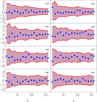
Figure 3: Angular-conic null test of isotropy applied to the Planck Commander 2015 temperature map, along with its mask. The plot shows the quantity $(\bar{\chi}^{2})_{l}^{L}$ versus $L$ for different angular multipoles $l$. The shaded contours represent $2\sigma$ cosmic variance from $10^{3}$ FFP6 simulations using the same mask. We also performed analyses with the other three Planck foreground-cleaned 2015 maps: SMICA, NILC, and SEVEM, obtaining qualitatively similar results.

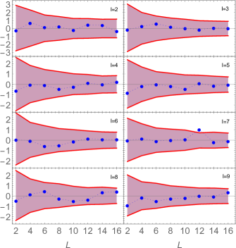
Figure 4: Angular-planar null test of isotropy applied to the Planck Commander 2015 temperature map, along with its mask. The plot shows the quantity $(\bar{\chi}^{2})_{l}^{L}$ versus $L$ for different angular multipoles $l$. The shaded contours represent $2\sigma$ cosmic variance from $10^{3}$ FFP6 simulations using the same mask. We also performed analyses with the other three Planck foreground-cleaned 2015 maps: SMICA, NILC, and SEVEM, obtaining qualitatively similar results. Note that, for this test, the planar multipole $L$ is always even.

In this section we perform a simple statistical analysis of the 2015 Planck data release Ade2015a using the tools we developed. While this analysis is not intended to be exhaustive, it offers an important sanity check of the available data. For these analyses we have used the Planck Commander 2015 temperature map, along with its mask. The data points were compared with the 1000 Full Focal Plane (FFP6) simulations provided by the Planck team, to which we have also applied the Commander-Ruler mask, so as to ensure that we are comparing quantities with the same foreground treatments. The results of our analysis are shown in Figs. (3) and (4), where the data points are compared to the $2\sigma$ cosmic variance bars from the FFP6 simulations. We have also performed analyses with the other three Planck foreground-cleaned 2015 maps: SMICA, NILC, and SEVEM, obtaining qualitatively similar results.

Our results show no drastic discrepancies between the Planck 2015 data and the $\Lambda$CDM model at the multipoles we tested, although it is interesting to note that the cases $(\overline{\chi}^{2})^{L}_{l=3}$ for the cone and $(\overline{\chi}^{2})^{L}_{l=4,5}$ for the disc present a consistent deficit of conic/planar modulations in the scales we considered. It is important to mention that, while the conic/planar multipoles $L$ are statistically independent in the $\Lambda$CDM model (see Eq. (33)), the angular multipoles $l$ are not. In other words, while the points in each frame of Figs. (3) and (4) are independent from each other, they are not independent from the points in other frames of the same figure. Given that there are 16 independent points in the multipole range we considered, on average, only $16\times 4.55\%=0.73$ of them should fall outside the $2\sigma$ ($95.45\%$ Cl) variance error bars. This analysis is in clear agreement with our findings.

IV Conclusions and Perspectives

The impressive agreement of the $\Lambda$CDM model with current CMB data compel us to go beyond the simple statistical framework of a Gaussian, homogeneous and isotropic universe. Assuming that CMB is Gaussian, a fact which is supported by the latest Planck data, hints of new physics can be found in the realm of statistical anisotropy – a possibility which is still open to debate.

In this work we have proposed two new representations of the 2pcf as alternatives to the popular bipolar power spectrum (BipoSH) analysis. Besides being model independent, these tools are entirely based on the geometry defined by the two unit vectors in the CMB sphere, namely, a cone and a disc. These tools differ from the BipoSH analysis in two main aspects. First, the new decompositions of the 2pcf are geometrically inspired, which means that null tests of isotropy based on their multipolar coefficients can help to elucidate the physical mechanism behind signals of anisotropy. We have illustrated this feature with concrete examples of anisotropic maps in which only one of these estimators will be non-zero. Thus, for example, a statistically significant detection of the angular-planar spectrum cannot result from parity-violating physics, since in this case the angular-planar spectrum is zero for all multipoles. Second, the clear geometrical role of the anisotropic degrees of freedom used as variables in the 2pcf allows us to construct simpler correlation functions whenever we have a more symmetric situation at hand. This feature has the important consequence of allowing us to reduce cosmic variance in a systematic way.

The angular-conic and angular-planar null tests of isotropy have not shown significant deviations of statistical isotropy in the lowest multipoles of the Planck data, although some angular multipoles presented interesting low conic/planar modulations. Our analysis does not reveal any new statistical anomaly, although known features, such as the hemispherical power anomaly, are expected to appear at higher angular multipoles $\l$, which were not included in our first analysis.

A more complete analysis of existing observational data, including a larger range of multipoles and a better assessment of systematics, is postponed to a future work. Of particular interest is the application of the angular-conic spectra in the investigation of the hemispherical power asymmetry found in Refs. Akrami2014 ; Bernui08 ; Bernui2014 . Indeed, these references considered a pixel-based variance estimator which resembles in many ways the conic degrees of freedom that we have introduced. In this respect, it is worth mentioning that the conic 2pcf might have some relevance for the detection of Baryonic Acoustic Oscillations. Indeed, the ring-like pattern that BAO produces in the distribution of galaxies leads exactly to a three-dimensional cone centred on the observer.

Appendix A

We present here the derivation of our main results, Eqs. (10) and (17). We also collect useful identities and mathematical formulas used in the text.

A.1 Spherical Harmonics and Wigner 3J symbols

Our definition for the spherical harmonics is

$$Y_{lm}(\chi,\phi)=(-1)^{m}\eta_{lm}P_{l}^{m}(\cos\chi)e^{im\phi}\,,$$

where

$$\eta_{lm}=\sqrt{\frac{2l+1}{4\pi}\frac{(l-m)!}{\left(l+m\right)!}}=\eta_{l,-m}\frac{(l-m)!}{(l+m)!}\,.$$ (37)

At the point $(\chi,\phi)=(\pi/2,\phi)$, it simplifies to

$$Y_{lm}(\pi/2,\phi)=\lambda_{lm}e^{im\phi}\,,$$ (38)

where

$$\lambda_{lm} =(-1)^{\frac{(l+m)}{2}}\times$$

$$\begin{cases}\!\left[\!\frac{2l+1}{4\pi}\frac{(l+m-1)!!}{(l+m)!!}\frac{(l-m-1)!!}{(l-m)!!}\!\right]^{1/2}\!\!&l+m=\textrm{even}\\ 0&\textrm{otherwise}\,.\end{cases}$$ (39)

The relation between Wigner 3Js and Clebsch-Gordan coefficients are

$$\left(\begin{array}[]{ccc}l_{1}&l_{2}&l_{3}\\ m_{1}&m_{2}&-m_{3}\end{array}\right)=\frac{(-1)^{l_{1}-l_{2}-m_{3}}}{\sqrt{2l_{3}+1}}C_{l_{1}m_{1}l_{2}m_{2}}^{l_{3}m_{3}}\,.$$ (40)

Other useful identities include

$$\sum_{m}(-1)^{l-m}\left(\begin{array}[]{ccc}L&l&l\\ 0&m&-m\end{array}\right) =\sqrt{2l+1}\delta_{L0}\,,$$ (43)

$$\left(\begin{array}[]{ccc}0&l&l\\ 0&m&-m\end{array}\right) =\frac{(-1)^{l-m}}{\sqrt{2l+1}}\,.$$ (46)

We also remind two useful orthogonality relations of the Wigner rotation matrices. These are

$$\int D^{l_{1}}_{m_{1}m^{\prime}_{1}}(w)D^{l_{2}*}_{m_{2}m^{\prime}_{2}}(w)dw=8\pi^{2}\delta_{\ell_{1}\ell_{2}}\delta_{m_{1}m_{2}}\delta_{m_{1}^{\prime}m_{2}^{\prime}}\,,$$

and

$$\int D^{l_{1}}_{m_{1}m^{\prime}_{1}}(w) D^{l_{2}}_{m_{2}m^{\prime}_{2}}(w)D^{l_{3}}_{m_{3}m^{\prime}_{3}}(w)dw=$$

$$8\pi^{2}\left(\begin{array}[]{ccc}l_{1}&l_{2}&l_{3}\\ m^{\prime}_{1}&m^{\prime}_{2}&m^{\prime}_{3}\end{array}\right)\left(\begin{array}[]{ccc}l_{1}&l_{2}&l_{3}\\ m_{1}&m_{2}&m_{3}\end{array}\right)\,,$$

with $w=(\alpha,\beta,\gamma)$ being the three Euler angles.

A.2 Derivation of Eq. (10) for conic-angular modulations

After expanding the 2pcf in terms of Legendre polynomials and Wigner $D$-matrices, we equate expressions (II.2) and (2). Since the 2pcf is a scalar, this equality should hold in a coordinate system in which the symmetry axis of the cone is aligned with the $z$-axis. That will mean:

$$\Theta=\Phi=\eta=0\,,\quad\chi_{1}=\chi_{2}=\chi/2\,,\quad\phi_{1}=\phi_{2}-\pi=0\,.$$

Using the identity $D_{MM^{\prime}}^{L}(0,0,0)=\delta_{MM^{\prime}}$ and the orthogonality of the Legendre polynomials, we then arrive at

$$\sum_{L,M}\frac{(2L+1)}{2\pi}{\cal C}_{l}^{LMM}=\sum_{\begin{subarray}{c}l_{1},m_{1}\\ l_{2},m_{2}\end{subarray}}\left\langle a_{l_{1}m_{1}}a_{l_{2}m_{2}}\right\rangle J_{l_{1}m_{1}l_{2}m_{2}}^{l}\,,$$ (47)

where $J_{l_{1}m_{1}l_{2}m_{2}}^{l}$ was defined in Eq. (12). If we now rotate the axes back to a general coordinate system using $\omega=\left\{\eta,\Theta,\Phi\right\}$ as the three Euler angles, the coefficients ${\cal C}_{l}^{LMM}$ and $a_{lm}$ will transform as Varshalovich1988a

$${\cal C}_{l}^{LMM}\!=\!\sum_{M^{\prime}}\tilde{{\cal C}}_{l}^{LMM^{\prime}}D_{MM^{\prime}}^{L}(\omega),\quad a_{lm}\!=\!\sum_{m^{\prime}}\tilde{a}_{lm^{\prime}}D_{mm^{\prime}}^{l}(\omega)\,.$$

Then, we multiply both sides of (47) by $D_{M^{\prime}M^{\prime\prime}}^{L^{\prime}}(\omega)$ and use the orthogonality of the Wigner rotation matrices to isolate $\tilde{{\cal C}}_{l}^{LMM^{\prime}}$. Finally, we use $(-1)^{M+M^{\prime}}\tilde{{\cal C}}_{l}^{L,-M,-M^{\prime}}=\tilde{{\cal C}}_{l}^{LMM^{\prime}*}$, which follows from the reality of the 2pcf, and substitute ${\cal C}_{l}^{LMM^{\prime}*}\rightarrow{\cal C}_{l}^{LMM^{\prime}}$, since we could equally well have started with the complex conjugate in the expansion (II.2). Dropping primes and tildes, we arrive at (10).

A.2.1 Isotropic limit

In order to derive the isotropic limit (13), we note that, in this limit, $\langle a_{\ell_{1}m_{1}}a_{\ell_{2}m_{2}}\rangle=(-1)^{m_{2}}C_{\ell_{1}}\delta_{\ell_{1}\ell_{2}}\delta_{m_{1},-m_{2}}$. Since the Wigner 3J symbol appearing in Eq. (10) is zero unless $M^{\prime}+m_{1}+m_{2}=0$, this implies that $M^{\prime}=0$. Then, using Eq. (43), we arrive at

$${\cal C}^{LMM^{\prime}}_{l}=2\pi\sum_{l_{1}}C_{l_{1}}(-1)^{l_{1}}\sqrt{2l_{1}+1}J^{lLM}_{l_{1}l_{1}}\times\delta_{L0}\delta_{M^{\prime}0}\,.$$ (48)

In the above expression, the non-vanishing terms of the coupling matrix are of the form $J^{l0M}_{l_{1}l_{2}}$. Combining Eq. (46) with the addition theorem for the associated Legendre polynomials one can show that

$$J^{l0M}_{l_{1}l_{2}}=\frac{(-1)^{l_{1}}}{\sqrt{2l_{1}+1}}\frac{1}{2\pi}\delta_{ll_{1}}\delta_{M0}\,.$$ (49)

Combining this result with (48), we finally get (13).

A.3 Derivation of Eq. (17) for planar-angular modulations

Equating the expanded 2pcf (16) with (2), we choose a particular coordinate system in which the normal to the disc points in the $z$-direction, which means:

$$\Theta=\Phi=\eta=0,\quad\chi_{1}=\chi_{2}=\pi/2,\quad\phi_{1}=0,\quad\chi=\phi_{2}\,.$$

Using $D_{M^{\prime}M}^{L}(0,0,0)=\delta_{M^{\prime}M}$, $Y_{lm}(\pi/2,\phi)=\lambda_{lm}e^{im\phi}$, and integrating over $P_{l}(\cos\chi)$, we find

$$\sum_{L,M}\frac{(2L+1)}{2\pi}{\cal D}_{l}^{LMM}=\sum_{\begin{subarray}{c}l_{1},m_{1}\\ l_{2},m_{2}\end{subarray}}\left\langle a_{l_{1}m_{1}}a_{l_{2}m_{2}}\right\rangle I_{l_{1}m_{1}l_{2}m_{2}}^{l}$$

where $I_{l_{1}m_{1}l_{2}m_{2}}^{l}$ was introduced in (19). We now rotate back to a general coordinate system using $\omega=\left\{\eta,\Theta,\Phi\right\}$ as the Euler angles and the fact that, under rotations

$${\cal D}_{l}^{LMM}\!=\!\sum_{M^{\prime}}\tilde{{\cal D}}_{l}^{LMM^{\prime}}D_{MM^{\prime}}^{L}(\omega),\quad a_{lm}\!=\!\sum_{m^{\prime}}\tilde{a}_{lm^{\prime}}D_{mm^{\prime}}^{l}(\omega)\,.$$

From this point on, the deduction is similar to the case of the cone. After some redefinitions and relabeling of the indices, we finally arrive at (17).

A.3.1 Isotropic limit

The derivation of (20) follows a similar deduction to the one of the angular-conic power spectrum. In this limit, the expression $\langle a_{\ell_{1}m_{1}}a_{\ell_{2}m_{2}}\rangle=(-1)^{m_{2}}C_{\ell_{1}}\delta_{\ell_{1}\ell_{2}}\delta_{m_{1},-m_{2}}$ implies that $M^{\prime}=0$. Then, using Eq. (43), we arrive at

$${\cal D}^{LMM^{\prime}}_{l}=2\pi\sum_{l_{1}}C_{l_{1}}(-1)^{l_{1}}\sqrt{2l_{1}+1}I^{lLM}_{l_{1}l_{1}}\times\delta_{L0}\delta_{M^{\prime}0}\,.$$ (50)

Using again Eq. (46), it is not difficult to show that

$$I^{l0M}_{l_{1}l_{2}}=\frac{(-1)^{l_{1}}}{\sqrt{2l_{1}+1}}\frac{1}{2\pi}\delta_{ll_{1}}\delta_{M0}\,.$$ (51)

Combining this result with (50), we finally get (20).

References

- (1) Planck, P. Ade et al., Astron.Astrophys. 571, A16 (2014), [1303.5076].
- (2) Planck, P. Ade et al., arXiv:1502.01589.
- (3) EUCLID Collaboration, R. Laureijs et al., arXiv:1110.3193.
- (4) LSST Dark Energy Science Collaboration, A. Abate et al., arXiv:1211.0310.
- (5) J-PAS Collaboration, N. Benitez et al., arXiv:1403.5237.
- (6) N. J. Cornish, D. N. Spergel, G. D. Starkman and E. Komatsu, Phys.Rev.Lett. 92, 201302 (2004), [astro-ph/0310233].
- (7) M. Kunz et al., Phys.Rev. D73, 023511 (2006), [astro-ph/0510164].
- (8) Planck Collaboration, P. Ade et al., arXiv:1502.01593.
- (9) O. Fabre, S. Prunet and J.-P. Uzan, arXiv:1311.3509.
- (10) F. Schmidt and L. Hui, Phys.Rev.Lett. 110, 011301 (2013), [1210.2965].
- (11) WMAP Collaboration, E. Komatsu et al., Astrophys.J.Suppl. 148, 119 (2003), [astro-ph/0302223].
- (12) Planck, P. Ade et al., Astron.Astrophys. 571, A24 (2014), [1303.5084].
- (13) Planck Collaboration, P. Ade et al., arXiv:1502.01592.
- (14) COrE Collaboration, F. Bouchet et al., arXiv:1102.2181.
- (15) C. J. Copi, D. Huterer, D. J. Schwarz and G. D. Starkman, Adv.Astron. 2010, 847541 (2010), [1004.5602].
- (16) C. Pitrou, T. S. Pereira and J.-P. Uzan, JCAP 0804, 004 (2008), [0801.3596].
- (17) D. Hanson, A. Lewis and A. Challinor, Phys.Rev. D81, 103003 (2010), [1003.0198].
- (18) C. Bennett et al., Astrophys.J.Suppl. 192, 17 (2011), [1001.4758].
- (19) A. Yoho, C. J. Copi, G. D. Starkman and T. S. Pereira, Mon.Not.Roy.Astron.Soc. 432, 2208 (2013).
- (20) Planck, P. Ade et al., Astron.Astrophys. 571, A23 (2014), [1303.5083].
- (21) L. Amendola et al., JCAP 1107, 027 (2011), [1008.1183].
- (22) T. Kahniashvili, G. Lavrelashvili and B. Ratra, Phys.Rev. D78, 063012 (2008), [0807.4239].
- (23) A. Bernui and W. Hipolito-Ricaldi, Mon.Not.Roy.Astron.Soc. 389, 1453 (2008), [0807.1076].
- (24) R. Durrer, T. Kahniashvili and A. Yates, Phys.Rev. D58, 123004 (1998), [astro-ph/9807089].
- (25) G. Hinshaw et al., Astrophys.J. 464, L25 (1996), [astro-ph/9601061].
- (26) WMAP, D. Spergel et al., Astrophys.J.Suppl. 148, 175 (2003), [astro-ph/0302209].
- (27) C. J. Copi, D. Huterer, D. J. Schwarz and G. D. Starkman, Phys.Rev. D75, 023507 (2007), [astro-ph/0605135].
- (28) C. J. Copi, D. Huterer, D. J. Schwarz and G. D. Starkman, Mon.Not.Roy.Astron.Soc. 399, 295 (2009), [0808.3767].
- (29) C. J. Copi, D. Huterer, D. J. Schwarz and G. D. Starkman, Adv.Astron. 2010, 847541 (2010), [1004.5602].
- (30) C. J. Copi, D. Huterer, D. J. Schwarz and G. D. Starkman, arXiv:1310.3831.
- (31) A. Hajian, astro-ph/0702723.
- (32) E. F. Bunn and A. Bourdon, Phys.Rev. D78, 123509 (2008), [0808.0341].
- (33) C. Copi, D. Huterer, D. Schwarz and G. Starkman, Mon.Not.Roy.Astron.Soc. 434, 3590 (2013), [1303.4786].
- (34) A. Yoho, C. Copi, G. Starkman and A. Kosowsky, Mon.Not.Roy.Astron.Soc. 442, 2392 (2014), [1310.7603].
- (35) A. Yoho, S. Aiola, C. J. Copi, A. Kosowsky and G. D. Starkman, arXiv:1503.05928.
- (36) D. A. Varshalovich, A. N. Moskalev and V. K. Khersonskii, Quantum theory of angular momentum (World Scientific, 1998).
- (37) A. Hajian and T. Souradeep, Astrophys.J. 597, L5 (2003), [astro-ph/0308001].
- (38) A. Hajian, T. Souradeep and N. J. Cornish, Astrophys.J. 618, L63 (2004), [astro-ph/0406354].
- (39) A. Hajian and T. Souradeep, astro-ph/0501001.
- (40) N. Joshi, S. Jhingan, T. Souradeep and A. Hajian, Phys.Rev. D81, 083012 (2010), [0912.3217].
- (41) L. G. Book, M. Kamionkowski and T. Souradeep, Phys.Rev. D85, 023010 (2012), [1109.2910].
- (42) M. Kamionkowski and T. Souradeep, Phys.Rev. D83, 027301 (2011), [1010.4304].
- (43) A. Hajian and T. Souradeep, Phys.Rev. D74, 123521 (2006), [astro-ph/0607153].
- (44) S. Kumar et al., arXiv:1409.4886.
- (45) A. R. Pullen and M. Kamionkowski, Phys.Rev. D76, 103529 (2007), [0709.1144].
- (46) T. S. Pereira and L. R. Abramo, Phys.Rev. D80, 063525 (2009), [0907.2340].
- (47) L. R. Abramo and T. S. Pereira, Adv.Astron. 2010, 378203 (2010), [1002.3173].
- (48) L. R. Abramo, A. Bernui and T. S. Pereira, JCAP 0912, 013 (2009), [0909.5395].
- (49) S. M. Carroll, C.-Y. Tseng and M. B. Wise, Phys. Rev. D81, 083501 (2010), [0811.1086].
- (50) S. Prunet, J.-P. Uzan, F. Bernardeau and T. Brunier, Phys. Rev. D71, 083508 (2005), [astro-ph/0406364].
- (51) T. Kahniashvili, G. Lavrelashvili and B. Ratra, Phys. Rev. D78, 063012 (2008), [0807.4239].
- (52) Y. Akrami et al., Astrophys.J. 784, L42 (2014), [1402.0870].
- (53) A. Bernui, Phys.Rev. D78, 063531 (2008), [0809.0934].
- (54) A. Bernui, A. Oliveira and T. S. Pereira, JCAP 1410, 041 (2014), [1404.2936].