An algorithm computing combinatorial specifications of permutation classes

Abstract.

This article presents a methodology that automatically derives a combinatorial specification for a permutation class $\mathcal{C}$, given its basis $B$ of excluded patterns and the set of simple permutations in $\mathcal{C}$, when these sets are both finite. This is achieved considering both pattern avoidance and pattern containment constraints in permutations. The obtained specification yields a system of equations satisfied by the generating function of $\mathcal{C}$, this system being always positive and algebraic. It also yields a uniform random sampler of permutations in $\mathcal{C}$. The method presented is fully algorithmic.

1. Introduction

Permutation classes (and the underlying pattern order on permutations) were defined in the seventies, and since then the enumeration of specific permutation classes (i.e., sets of permutations closed under taking patterns) has received a lot of attention. In this context, as in many in combinatorics, a recursive description of the permutations belonging to the class is often the key towards their enumeration. This recursive description is a priori specific to the class studied. But more recently, the substitution decomposition (along with other general frameworks, see [Vat15, and references therein]) has been introduced for the study of permutation classes: it provides a general and systematic approach to their study, with a recursive point of view. This tool has already proved useful in solving many enumerative problems [AA05, AAB11, AB14, ASV12, among others], but also in other areas like algorithmics [BBCP07, BR06].

The goal of the current paper is to systematize even more the use of substitution decomposition for describing recursively and enumerating permutation classes. Our main result is an algorithm that computes a combinatorial specification (in the sense of Flajolet and Sedgewick [FS09]) for any permutation class containing finitely many simple permutations. Note that this problem has been addressed already in [AA05, BHV08], however with much less focus on the algorithmic side. Moreover, we introduce in this article a generalization of permutation classes that we call restrictions: while every permutation class is characterized by a set of forbidden patterns, a restriction is described giving a set of forbidden patterns and a set of mandatory patterns. Our algorithm also allows to compute a specification for restrictions containing finitely many simple permutations.

The article is organized as follows. We start by recalling the necessary background in Section 2: permutation classes, substitution decomposition, and the symbolic method. Section 3 gives a more detailed presentation of our results. Here, we dedicate specific attention to explaining the differences between our work and those of [AA05, BHV08], and to putting our result in a more global algorithmic context (namely, we describe an algorithmic chain from the basis $B$ of a class $\mathcal{C}$ to random sampling of permutations in $\mathcal{C}$). With the next sections, we enter the technical part of our work. After briefly solving the case of substitution-closed classes in Section 4, we explain in two steps how to obtain a combinatorial specification for other classes $\mathcal{C}$. Section 5 gives an algorithm producing an ambiguous system of combinatorial equations describing $\mathcal{C}$. Next, Section 6 describes how to adapt this algorithm to obtain a combinatorial specification for $\mathcal{C}$. Finally, Section 7 illustrates the whole process on examples.

2. Some background on permutations and combinatorial specifications

2.1. Permutation patterns and permutation classes

A permutation $\sigma$ of size $|\sigma|=n$ is a bijective map from $[1..n]=\{1,\ldots,n\}$ to itself. We represent a permutation by a word $\sigma=\sigma_{1}\sigma_{2}\ldots\sigma_{n}$, where each letter $\sigma_{i}$ denotes the image of $i$ under $\sigma$. We denote $\varepsilon$ the only permutation of size $0$; $\varepsilon$ is also called the empty permutation.

Definition 2.1.

For any sequence $s$ of $k$ distinct integers, the normalization of $s$ is the permutation $\pi$ of size $k$ which is order-isomorphic to $s$, i.e., $s_{\ell}<s_{m}$ whenever $\pi_{\ell}<\pi_{m}$.

For any permutation $\sigma$ of size $n$, and any subset $I=\{i_{1},\ldots,i_{k}\}$ of $\{1,\ldots,n\}$ with $i_{1}<\ldots<i_{k}$, $\sigma_{I}$ denotes the permutation of size $k$ obtained by normalization of the sequence $\sigma_{i_{1}}\ldots\sigma_{i_{k}}$.

Definition 2.2.

A permutation $\pi$ is a pattern of a permutation $\sigma$ if and only if there exists a subset $I$ of $\{1,\ldots,|\sigma|\}$ such that $\sigma_{I}=\pi$. We also say that $\sigma$ contains or involves $\pi$, and we write $\pi\preccurlyeq\sigma$. A permutation $\sigma$ that does not contain $\pi$ as a pattern is said to avoid $\pi$.

Example 2.3.

The permutation $\sigma=316452$ contains the pattern $2431$ whose occurrences are $3642$ and $3652$. But $\sigma$ avoids the pattern $2413$ as none of its subsequences of length $4$ is order-isomorphic to $2413$.

The pattern containment relation $\preccurlyeq$ is a partial order on permutations, and permutation classes are downsets under this order. In other words:

Definition 2.4.

A set $\mathcal{C}$ of permutations is a permutation class if and only if for any $\sigma\in\mathcal{C}$, if $\pi\preccurlyeq\sigma$, then we also have $\pi\in\mathcal{C}$.

Throughout this article, we take the convention that a permutation class only contains permutations of size $n\geq 1$, i.e., $\varepsilon\notin\mathcal{C}$ for any permutation class $\mathcal{C}$.

Every permutation class $\mathcal{C}$ can be characterized by a unique antichain $B$ (i.e., a unique set of pairwise incomparable elements) such that a permutation $\sigma$ belongs to $\mathcal{C}$ if and only if it avoids every pattern in $B$ (see for example [AA05]). The antichain $B$ is called the basis of $\mathcal{C}$, and we write $\mathcal{C}=Av(B)$. The basis of a class $\mathcal{C}$ may be finite or infinite; it is described as the permutations that do not belong to $\mathcal{C}$ and that are minimal in the sense of $\preccurlyeq$ for this criterion.

2.2. Simple permutations and substitution decomposition of permutations

The description of permutations in the framework of constructible structures (see Section 2.3) that will be used in this article relies on the substitution decomposition of permutations. Substitution decomposition is a general method, adapted to various families of discrete objects [MR84], that is based on core items and relations, and in which every object can be recursively decomposed into core objects using relations. In the case of permutations, the core elements are simple permutations and the relations are substitutions.

Definition 2.5.

An interval of a permutation $\sigma$ of size $n$ is a non-empty subset $\{i,\ldots,(i+\ell-1)\}$ of consecutive integers of $\{1,\ldots,n\}$ whose images by $\sigma$ also form a set of consecutive integers. The trivial intervals of $\sigma$ are $\{1\},\ldots,\{n\}$ and $\{1,\ldots,n\}$. The other intervals of $\sigma$ are called proper.

Definition 2.6.

A block (resp. normalized block) of a permutation $\sigma$ is any sequence $\sigma_{i_{1}}\ldots\sigma_{i_{m}}$ (resp. any permutation $\sigma_{I}$) for $I=\{i_{1},\ldots,i_{m}\}$ an interval of $\sigma$.

Definition 2.7.

A permutation $\sigma$ is simple when it is of size at least $4$ and it contains no interval, except the trivial ones.

Note that no permutation of size $3$ has only trivial intervals (so that the condition on the size is equivalent to “at least $3$”).

Remark 2.8.

The permutations $1$, $12$ and $21$ also have only trivial intervals, and are considered simple in many articles. Nevertheless, for our notational convenience in this work, we prefer to consider that they are not simple.

For a detailed study of simple permutations, in particular from an enumerative point of view, we refer the reader to [AA05, AAK03, Bri10]. Let us only mention that the number of simple permutations of size $n$ is asymptotically equivalent to $\frac{n!}{e^{2}}$ as $n$ grows.

Let $\sigma$ be a permutation of size $n$ and $\pi^{1},\ldots,\pi^{n}$ be $n$ permutations of size $p_{1},\ldots,p_{n}$ respectively. Define the substitution $\sigma[\pi^{1},\pi^{2},\ldots,\pi^{n}]$ of $\pi^{1},\pi^{2},\ldots,\pi^{n}$ in $\sigma$ (also called inflation in [AA05]) to be the permutation obtained by concatenation of $n$ sequences of integers $S^{1},\ldots,S^{n}$ from left to right, such that for every $i,j$, the integers of $S^{i}$ form a block, are ordered in a sequence order-isomorphic to $\pi^{i}$, and $S^{i}$ consists of integers smaller than $S^{j}$ if and only if $\sigma_{i}<\sigma_{j}$. The interested reader may find a formal definition in [Pie13, Definition 0.25]. When a permutation $\tau$ may be written as $\tau=\sigma[\pi^{1},\pi^{2},\ldots,\pi^{n}]$, we also say that $\sigma[\pi^{1},\pi^{2},\ldots,\pi^{n}]$ provides a block decomposition of $\tau$.

Example 2.9.

The substitution $1\,3\,2[2\,1,1\,3\,2,1]$ gives the permutation $2\,1\,\,4\,6\,5\,\,3$. In particular, $1\,3\,2[2\,1,1\,3\,2,1]$ is a block decomposition of $2\,1\,4\,6\,5\,3$.

When substituting in $\sigma=12$ or $21$, we often use $\oplus$ (resp. $\ominus$) to denote the permutation $12$ (resp. $21$).

Definition 2.10.

A permutation $\pi$ is $\oplus$-indecomposable (resp. $\ominus$-indecomposable) if it cannot be written as $\oplus[\pi^{1},\pi^{2}]$ (resp. $\ominus[\pi^{1},\pi^{2}]$).

Simple permutations, together with $\oplus$ and $\ominus$, are enough to describe all permutations through their substitution decomposition:

Theorem 2.11 (Proposition 2 of [AA05]).

Every permutation $\pi$ of size $n$ with $n\geq 2$ can be uniquely decomposed as either:

• $\oplus[\pi^{1},\pi^{2}]$, with $\pi^{1}$ $\oplus$-indecomposable,

• $\ominus[\pi^{1},\pi^{2}]$, with $\pi^{1}$ $\ominus$-indecomposable,

• $\sigma[\pi^{1},\pi^{2},\ldots,\pi^{k}]$ with $\sigma$ a simple permutation of size $k$.

Remark 2.12.

The simple permutation $\sigma$ in the third item of Theorem 2.11 is a pattern of the permutation $\pi$. Hence, as soon as $\pi$ belongs to some permutation class $\mathcal{C}$, then so does $\sigma$.

Theorem 2.11 provides the first step in the decomposition of a permutation $\pi$. To obtain its full decomposition, we can recursively decompose the permutations $\pi^{i}$ in the same fashion, until we reach permutations of size $1$. This recursive decomposition can naturally be represented by a tree, that is called the substitution decomposition tree (or decomposition tree for short) of $\pi$.

Definition 2.13.

The substitution decomposition tree $T$ of a permutation $\pi$ is the unique ordered tree encoding the substitution decomposition of $\pi$, where each internal node is either labeled by $\oplus,\ominus$ – those nodes are called linear – or by a simple permutation $\sigma$ – prime nodes.

Note that in decomposition trees, linear nodes are always binary, and the left child of a node labeled by $\oplus$ (resp. $\ominus$) may not be labeled $\oplus$ (resp. $\ominus$), since $\pi^{1}$ is $\oplus$-indecomposable (resp. $\ominus$-indecomposable) in the first (resp. second) item of Theorem 2.11.

Example 2.14.

The permutation $\pi=6\,9\,8\,7\,3\,11\,5\,4\,10\,17\,1\,2\,14\,16\,13\,15\,12$ can be recursively decomposed as

$$\pi = 2413[476519328,1,12,35241]$$

$$= 2413[31524[\oplus[1,\ominus[1,\ominus[1,1]]],1,1,\ominus[1,1],1]],1,\oplus[1,1],\ominus[2413[1,1,1,1],1]]$$

and its decomposition tree is given in Figure 1.

Figure 1. Decomposition tree of $\pi=6\ 9\ 8\ 7\ 3\ 11\ 5\ 4\ 10\ 17\ 1\ 2\ 14\ 16\ 13\ 15\ 12$.

Definition 2.15.

The substitution closure $\hat{\mathcal{C}}$ of a permutation class $\mathcal{C}$ is defined as $\cup_{k\geq 1}\mathcal{C}^{k}$ where $\mathcal{C}^{1}=\mathcal{C}$ and $\mathcal{C}^{k+1}=\{\sigma[\pi^{1},\ldots,\pi^{n}]\mid\sigma\in\mathcal{C}\textrm{ and }\pi^{i}\in\mathcal{C}^{k}\textrm{ for any }i\textrm{ from }1\textrm{ to }n=|\sigma|\}$.

Because simple permutations contain no proper intervals, we have:

Remark 2.16.

For any class $\mathcal{C}$, the simple permutations in ${\hat{\mathcal{C}}}$ are exactly the simple permutations in $\mathcal{C}$.

Consequently, for any permutation class $\mathcal{C}$, this allows to describe ${\hat{\mathcal{C}}}$ as the class of all permutations whose decomposition trees can be built on the set of nodes $\{\oplus,\ominus\}\cup\mathcal{S}_{\mathcal{C}}$, where $\mathcal{S}_{\mathcal{C}}$ denotes the set of simple permutations in $\mathcal{C}$ (if $12$ and $21$ belong to $\mathcal{C}$; otherwise we have to remove $\oplus$ or $\ominus$ from the set of nodes).

Definition 2.17.

A permutation class $\mathcal{C}$ is substitution-closed if $\mathcal{C}=\hat{\mathcal{C}}$, or equivalently if for every permutation $\sigma$ of $\mathcal{C}$, and every permutations $\pi^{1},\pi^{2},\ldots,\pi^{n}$ of $\mathcal{C}$ (with $n=|\sigma|$), the permutation $\sigma[\pi^{1},\pi^{2},\ldots,\pi^{n}]$ also belongs to $\mathcal{C}$.

Like before, a substitution-closed permutation class can therefore be seen as the set of decomposition trees built on the set of nodes $\{\oplus,\ominus\}\cup\mathcal{S}_{\mathcal{C}}$ (if $12$ and $21$ belong to $\mathcal{C}$; but otherwise $\mathcal{C}$ is trivial and has at most one permutation of each size).

Remark 2.18.

In [AA05], it is proven that substitution-closed permutation classes can be characterized as the permutation classes $Av(B)$ whose basis $B$ contains only simple permutations (or maybe $12$ or $21$ for trivial classes).

2.3. From combinatorial specifications to generating functions and random samplers

Let us leave aside permutations for now, and review some basics of the symbolic method about constructible structures and their description by combinatorial specifications. We will see in Theorem 6.4 (p.6.4) that the classes of permutations we are interested in fit in this general framework.

A class $\mathcal{C}$ of combinatorial structures is a set of discrete objects equipped with a notion of size: the size is a function of $\mathcal{C}\rightarrow\mathbb{N}$ denoted $|\cdot|$ such that for any $n$ the number of objects of size $n$ in $\mathcal{C}$ is finite.

Among the combinatorial structures, we focus on constructible ones, from the framework introduced in [FS09]. Basically, a constructible combinatorial class is a set of structures that can be defined from atomic structures of size $1$ (denoted by $\mathcal{Z}$), possibly structures of size $0$ (denoted by $\mathcal{E}$), and assembled by means of admissible constructors. While a complete list of these combinatorial constructors is given in [FS09], we only use a (small) subset of them: the disjoint union, denoted by $\uplus$ or $+$ (we may also use the notation $\sum$), to choose between structures; and the Cartesian product, denoted by $\times$, to form pairs of structures. More formally, a constructible combinatorial class is one that admits a combinatorial specification.

Definition 2.19.

A combinatorial specification for a combinatorial class $\mathcal{C}_{1}$ is an equation or a system of equations of the form

$$\begin{cases}\mathcal{C}_{1}&\!\!=~{}\mathcal{H}_{1}(\mathcal{E},\mathcal{Z},\mathcal{C}_{1},\mathcal{C}_{2},\dots,\mathcal{C}_{m}),\\ \mathcal{C}_{2}&\!\!=~{}\mathcal{H}_{2}(\mathcal{E},\mathcal{Z},\mathcal{C}_{1},\mathcal{C}_{2},\dots,\mathcal{C}_{m}),\\ &\phantom{=H_{k}}\vdots\\ \mathcal{C}_{m}&\!\!=~{}\mathcal{H}_{m}(\mathcal{E},\mathcal{Z},\mathcal{C}_{1},\mathcal{C}_{2},\dots,\mathcal{C}_{m}),\end{cases}$$

where each $\mathcal{H}_{i}$ denotes a term built from $\mathcal{C}_{1},\dots,\mathcal{C}_{m},\mathcal{Z}$ and $\mathcal{E}$ using admissible constructors.

For example, the equation $\mathcal{I}=\mathcal{E}+\mathcal{Z}\times\mathcal{I}$ describes a class $\mathcal{I}$ whose elements are finite sequences of atoms.

In this framework, the size of a combinatorial structure is its number of atoms ($\mathcal{Z}$) and from there, combinatorial structures can be counted according to their size. The size information for a whole combinatorial class, say $\mathcal{C}$, is encoded by its ordinary generating function, which is the formal power series $C(z)=\sum_{n\geq 0}c_{n}z^{n}$ where the coefficient $c_{n}$ is the number of structures of size $n$ in $\mathcal{C}$. Note that we also have $C(z)=\sum_{\pi\in\mathcal{C}}z^{|\pi|}$.

Combinatorial specifications of combinatorial classes may be automatically translated into systems defining their generating function (possibly implicitly). This system is obtained by means of a dictionary that associates an operator on generating functions to each admissible constructor. The complete dictionary is given in [FS09], together with the proof that this translation from constructors of combinatorial classes to operators on their generating functions is correct. Here, we only use the constructors disjoint union and Cartesian product, which are respectively translated to sum and product of generating functions.

A lot of information can be extracted from such functional systems; in particular, one can compute as many coefficients of the series as required, and [FS09] provides many tools to get asymptotic equivalents for these coefficients.

Combinatorial specifications may also be automatically translated into uniform random samplers of objects in the class described by the specification. Indeed, a specification can be seen as a (recursive) procedure to produce combinatorial objects, and randomizing the choices made during this procedure transforms the specification into a random sampler. To ensure that such random samplers are uniform (i.e. that for any $n$, two objects of the same size $n$ have the same probability of being produced), two methods have been developed: the recursive method [FZVC94] and the Boltzmann method [DFLS04]. In the first one, the coefficients of the generating functions are used for the probabilistic choices to ensure uniformity, making this method well-adapted for generating a large sample of objects of relatively small size: this requires to compute only once a relatively small number of coefficients. The focus of the second one is to achieve efficiently the generation of very large objects, with a small tolerance (of a few percents) allowed on their size. Coefficients of the generating functions are not needed in Boltzmann samplers, but rather the generating functions themselves. More precisely, the value of the generating function at a given point needs to be computed, and this is solved in [PSS12].

3. Our results in existing context

3.1. Our contributions, and comparison with [AA05, BHV08]

The goal of the present work is to solve algorithmically a combinatorial problem on permutation classes: computing in an automatic way a combinatorial specification for any given class, under some conditions specified below. We first have to determine how to describe the permutation class $\mathcal{C}$ in input. In all what follows, we will suppose that $\mathcal{C}$ is given by its basis $B$ of excluded patterns and the set $\mathcal{S}_{\mathcal{C}}$ of simple permutations in $\mathcal{C}$, assuming that both these sets are finite. Note that from [AA05, Theorem 9] the basis of $\mathcal{C}$ is necessarily finite when $\mathcal{C}$ contains finitely many simple permutations. On the other hand, from [BRV08, BBPR15], it is enough to know $B$ to decide whether $\mathcal{S}_{\mathcal{C}}$ is finite and (in the affirmative) to compute $\mathcal{S}_{\mathcal{C}}$ [PR12].

Our work is a continuation of the main result (Theorem 10) of [AA05]: every permutation class containing finitely many simples has an algebraic generating function. The main step in the proof of this result is to construct a system of combinatorial equations describing $\mathcal{C}$ using the substitution decomposition, and more precisely by propagation of pattern avoidance constraints in the decomposition trees. Although the proof is in essence constructive, there is still some work to be done to fully automatize this process. In Section 5, we review their method, going deeper in the details of the construction. This allows us to bring their methodology to a full algorithm – see Algorithm AmbiguousSystem (p.1) and Theorem 5.1 (p.5.1).

It is important to note that the description of $\mathcal{C}$ obtained in this way is not a combinatorial specification, since it is a priori ambiguous (that is to say, unions are not necessarily disjoint). Nevertheless, as it is done in [AA05], this ambiguous system can be used for proving the algebraicity of the generating function of $\mathcal{C}$, and even allows its computation (or implicit determination, in less favorable cases): it is enough to apply the inclusion-exclusion principle. The advantage of a specification over an ambiguous system will be discussed in Section 3.2 (fifth step, p.3.2).

The algebraicity result of [AA05] was re-proved in [BHV08] and extended to generating functions of some subsets of classes $\mathcal{C}$ with finitely many simples: the alternating permutations in $\mathcal{C}$, the even ones, the involutions in $\mathcal{C}$, … For our purpose, those extensions are less important than the alternative proof of the main result of [AA05]: indeed, this second proof describes a method to build a combinatorial specification for $\mathcal{C}$. Essential to this proof are query-complete sets, whose definition we recall.

Definition 3.1.

A property is any set $P$ of permutations. A permutation $\pi$ is said to satisfy $P$ when $\pi\in P$. A set $\mathcal{P}$ of properties is query-complete if, for every simple permutation $\sigma$ (and also for $\sigma=\oplus$ or $\ominus$) and for every property $P\in\mathcal{P}$, it can be decided whether $\sigma[\alpha_{1},\dots,\alpha_{|\sigma|}]$ satisfies $P$ knowing only which properties of $\mathcal{P}$ are satisfied by each $\alpha_{i}$.

The proof of the main result (Theorem 1.1) of [BHV08] shows that a combinatorial specification for a permutation class $\mathcal{C}$ with finitely many simples can be obtained from any finite query-complete set $\mathcal{P}$ such that $\mathcal{C}\in\mathcal{P}$. More precisely, this combinatorial specification consists of three types of equations, described below (this is reduced to two types by plugging the third one into the second one). Recall that $\mathcal{S}_{\mathcal{C}}$ denotes the set of simple permutations in $\mathcal{C}$. Note that all unions below are finite, since $\mathcal{P}$ and $\mathcal{S}_{\mathcal{C}}$ are finite by assumption.

• First, $\mathcal{C}$ is written as the disjoint union

  $$\mathcal{C}=\uplus\,\mathcal{C}_{\mathcal{X}},$$

  where the union runs over all subsets $\mathcal{X}$ of $\mathcal{P}$ containing $\mathcal{C}$ with $\mathcal{C}_{\mathcal{X}}$ denoting the set of permutations that satisfy every property in $\mathcal{X}$ and do not satisfy any property in $\mathcal{P}\setminus\mathcal{X}$.

• Second, for any such set $\mathcal{X}$, the substitution decomposition allows to write

  $$\mathcal{C}_{\mathcal{X}}=1_{\mathcal{X}}\uplus\mathcal{C}_{\mathcal{X}}^{\oplus}\uplus\mathcal{C}_{\mathcal{X}}^{\ominus}\uplus\biguplus_{\sigma\in{\mathcal{S}}_{\mathcal{C}}}\mathcal{C}_{\mathcal{X}}^{\sigma}$$

  where $1_{\mathcal{X}}$ is either the set $\{1\}$ if the permutation $1$ belongs to $\mathcal{C}_{\mathcal{X}}$, or the empty set otherwise, and where $\mathcal{C}_{\mathcal{X}}^{\sigma}$ is the subset of $\mathcal{C}_{\mathcal{X}}$ of permutations whose decomposition tree has root $\sigma$.

• And third, for $\sigma\in\{\oplus,\ominus\}\cup{\mathcal{S}}_{\mathcal{C}}$ and $\mathcal{X}$ as above, the fact that $\mathcal{P}$ is query-complete allows to express $\mathcal{C}_{\mathcal{X}}^{\sigma}$ as

  $$\mathcal{C}_{\mathcal{X}}^{\sigma}=\biguplus\sigma[\mathcal{C}_{\mathcal{X}_{1}},\dots,\mathcal{C}_{\mathcal{X}_{m}}]$$

  where the union is over the set $E_{\mathcal{X},\sigma}$ of all $m$-uples $(\mathcal{X}_{1},\dots,\mathcal{X}_{m})$ of subsets of $\mathcal{P}$ such that if, for every $i\in[1..m]$, it holds that $\alpha_{i}\in\mathcal{C}_{\mathcal{X}_{i}}$ then $\sigma[\alpha_{1},\dots,\alpha_{m}]\in\mathcal{C}_{\mathcal{X}}$. In the case where $\sigma=\oplus$ (resp. $\ominus$), to ensure uniqueness of the decomposition, we further need to enforce that $\mathcal{X}_{1}$ contains the property of being $\oplus$-indecomposable (resp. $\ominus$-indecomposable). W.l.o.g., we can assume that these properties are in $\mathcal{P}$.

Note that the number of equations in the specification obtained depends exponentially on the size of $\mathcal{P}$, since there is at least one equation for each subset of $\mathcal{P}$ containing $\mathcal{C}$. Similarly, the number of terms of the union defining some $\mathcal{C}_{\mathcal{X}}^{\sigma}$ may be exponential in the size of $\mathcal{P}$, since the union is over $m$-uples of subsets of $\mathcal{P}$ (with $m=|\sigma|$).

We point out that the above specification is not fully explicit (even assuming that $\mathcal{P}$ is given), since there is no explicit description of the sets $E_{\mathcal{X},\sigma}$. As explained in the proof of Lemma 2.1 of [BHV08], the sets $E_{\mathcal{X},\sigma}$ may be described using so-called lenient inflations, which are intimately linked with the embeddings by blocks of [AA05]. But neither [BHV08] nor [AA05] discuss their effective computation. We will return to this problem later in this section.

For any permutation class $\mathcal{C}=Av(B)$ with finitely many simples, the authors of [BHV08] provide a finite query-complete set that contains $\mathcal{C}$, and conclude that there is a combinatorial specification for any such $\mathcal{C}$. More precisely, the class $\mathcal{C}$ being described as $\cap_{\beta\in B}Av(\beta)$, they rather consider separately every principal class $Av(\beta)$ for all $\beta\in B$, and define a finite query-complete set $\mathcal{P}_{\beta}$ containing it. This is essentially their Lemma 2.1. The query complete set associated with $\mathcal{C}$, denoted $\mathcal{P}_{\mathcal{C}}$, is then obtained taking the union of all $\mathcal{P}_{\beta}$. It consists of the following properties: the set of $\oplus$-indecomposable permutations, the set of $\ominus$-indecomposable permutations, and the set $Av(\rho)$ for every permutation $\rho$ which is a pattern of some $\beta\in B$. Thus $\mathcal{P}_{\mathcal{C}}$ is often a big set.

It should be noticed that the query-complete sets that are used in the examples of [BHV08, Section 4] are however strictly included in the set $\mathcal{P}_{\mathcal{C}}$. These smaller query-complete sets are better, since they result in specifications with fewer equations and unions having fewer terms than the ones that would be obtained applying to the letter the specializations of the proofs. But there are no indications in [BHV08] on how these smaller query-complete sets were computed, nor on how this could generalize to other examples. It should be noticed that in the examples of [BHV08], the class is either substitution-closed, or contains no simple permutations.

To summarize, the proof of the main result of [BHV08] gives a general method to compute a specification for a permutation class having finitely many simple permutations. But there is still some work to be done to fully automatize this process, and the specification obtained would be very big in general. Moreover, an algorithm using this method would have a lot of computations to do (the computation of all the sets $E_{\mathcal{X},\sigma}$). On the other hand, the ad hoc constructions of the examples of [BHV08] show that using the specificity of a particular permutation class, it is possible to obtain shorter specifications with fewer computations.

Our main contribution is to give an algorithm to compute a specification for any permutation class having finitely many simples, using a different approach – see Algorithm Specification (p.6) and Theorem 6.4 (p.6.4). Our method is general (unlike the ad hoc methods used in the examples of [BHV08]) but nevertheless uses the specificity of the permutation class given in input (unlike the method described in the proofs of [BHV08]) in order to do less computations and to have fewer equations in the specification.

Even if the method we use and the specification we produce are not exactly the ones presented by [BHV08] and reviewed above, they have some similarities. When considering the partition of $\mathcal{C}$ into $\uplus\,\mathcal{C}_{\mathcal{X}}$ shown above, [BHV08] is looking at a very fine level of details, where a coarser level could be enough. With our method, we consider the partition of $\mathcal{C}$ which is the coarsest possible to allow the derivation of a specification. In practice, if two sets $\mathcal{X}$ and $\mathcal{X}^{\prime}$ are such that $\mathcal{C}_{\mathcal{X}}$ and $\mathcal{C}_{\mathcal{X}^{\prime}}$ appear as $\mathcal{C}_{\mathcal{X}}\uplus\mathcal{C}_{\mathcal{X}^{\prime}}$ everywhere in the specification resulting from [BHV08], our specification will have only one term instead of these two, representing $\mathcal{C}_{\mathcal{X}}\uplus\mathcal{C}_{\mathcal{X}^{\prime}}$. Of course, this holds for unions with more terms as well. Considering fewer sets $\mathcal{X}$ results in fewer equations in the specification, fewer terms in the unions and fewer sets $E_{\mathcal{X},\sigma}$. Since the computation of the $E_{\mathcal{X},\sigma}$ amounts to computing the specification from the query-complete set, the algorithmic complexity for computing the specification with our method is hereby reduced, compared to what a formalized algorithm of the approach of [BHV08] would give.

Concretely, our algorithm computes a query-complete set, the sets $E_{\mathcal{X},\sigma}$ associated, and the specification in parallel, whereas the method of [BHV08] is to first compute a query-complete set and then deduce a specification. Note that in our presentation, the result of our algorithm is only the specification, but it contains also implicitly the description of the query-complete set and of the $E_{\mathcal{X},\sigma}$.

To obtain the announced coarsest partition of $\mathcal{C}$, and the subsequent specification with as few equations as possible that it yields, we proceed as follows. We use the same guideline as in [AA05] for computing a possibly ambiguous combinatorial system describing $\mathcal{C}$ (however making this approach effective): the essential idea is to use the substitution decomposition and to propagate pattern avoidance constraints in the decomposition trees. We get rid of the ambiguity by introducing complement sets, but only when they are needed (the method in the proofs of [BHV08] can be seen as somehow introducing all complement sets at once). In practice, it means that we are not only propagating avoidance constraints in decomposition trees, but also containment constraints. It will be clear in Sections 5 and 6 that even though the purposes of those two types of constraint are opposite, the ways to propagate them are very similar, an essential step being the effective computation of the embeddings/lenient inflations mentioned in [AA05, BHV08]. The method used to explicitly determine which avoidance/containment constraints are necessary and to effectively propagate them in the trees is completely new with respect to [AA05, BHV08].

To conclude on our contributions compared with those of [AA05, BHV08], our work describes how to obtain a combinatorial specification for any class having finitely many simple permutations. Contrary to [AA05, BHV08], our work is fully algorithmic. Moreover, we develop a method allowing to have fewer equations in the specification and to have a better efficiency compared to what a formalized algorithm of the approach of [BHV08] would give.

3.2. An algorithmic chain from $B$ to random permutations in $Av(B)$

Our main result (that is, the algorithmic computation of specifications for permutation classes with finitely many simples) can and should be viewed in the context of other recent algorithms from the literature. Together, they provide a full algorithmic chain starting with the finite basis $B$ of a permutation class $\mathcal{C}$, and computing a specification for $\mathcal{C}$, from which it is possible to sample permutations in $\mathcal{C}$ uniformly at random. Figure 2 shows an overview of this algorithmic chain, and we present its main steps below. Note that this procedure may fail to compute its final result, namely when $\mathcal{C}$ contains an infinite number of simple permutations, this condition being tested algorithmically.

Figure 2. The full algorithmic chain starting from the basis $B$ of a permutation class $\mathcal{C}$, with complexities given w.r.t. $n=\sum_{\beta\in B}|\beta|$, $k=|B|$, $p=\max\{|\beta|:\beta\in B\}$, $N=|\mathcal{S}_{\mathcal{C}}|$ and $\ell=\max\{|\pi|:\pi\in\mathcal{S}_{\mathcal{C}}\}$ where $\mathcal{S}_{\mathcal{C}}$ is the set of simple permutations of $\mathcal{C}$.

We have chosen that the permutation class in input of our procedure should be given by its basis $B$, that we require to be finite. This does not cover the whole range of permutation classes, but it is one of the possible ways to give a finite input to our algorithm. There are of course other finite descriptions of permutation classes, even of some with infinite basis (by a recognition procedure for example). The assumption of the description by a finite basis has been preferred for two reasons: first, it encompasses most of the permutation classes that have been studied; and second, it is a necessary condition for classes to contain finitely many simple permutations (see [AA05, Theorem 9]) and hence for our algorithm to succeed.

First step: Finite number of simple permutations.
First, we check whether $\mathcal{C}=Av(B)$ contains only a finite number of simple permutations. This is achieved using algorithms of [BBPR10] when the class is substitution-closed and of [BBPR15] otherwise. The complexity of these algorithms is respectively $\mathcal{O}(n\log n)$ and $\mathcal{O}(n\log n+p^{2k})$, where $n=\sum_{\beta\in B}|\beta|$, $p=\max\{|\beta|:\beta\in B\}$ and $k=|B|$.

Second step: Computing simple permutations.
The second step of the algorithm is the computation of the set of simple permutations $\mathcal{S}_{\mathcal{C}}$ contained in $\mathcal{C}=Av(B)$, when we know it is finite. Again, when $\mathcal{C}$ is substitution-closed, $\mathcal{S}_{\mathcal{C}}$ can be computed by an algorithm that is more efficient than in the general case. The two algorithms are described in [PR12], and their complexity depends on the output: $\mathcal{O}(N\cdot\ell^{p+2}\cdot k)$ in general and $\mathcal{O}(N\cdot\ell^{4})$ for substitution-closed classes, with $N=|\mathcal{S}_{\mathcal{C}}|$, $p=\max\{|\beta|:\beta\in B\}$, $\ell=\max\{|\pi|:\pi\in\mathcal{S}_{\mathcal{C}}\}$ and $k=|B|$.

In the case of substitution-closed classes, the set of simple permutations in $\mathcal{C}$ gives an immediate access to a specification for $\mathcal{C}$ – see [AA05] or Theorem 4.3 (p.4.3). In the general case, finding such a specification is the algorithmic problem that we address in this article.

Third step: Computing a combinatorial specification.
This corresponds to the computation of a combinatorial specification for $\mathcal{C}$ by propagation of pattern constraints and disambiguation of the equations, as briefly presented in Section 3.1 and described in details in Sections 5 and 6.

From a combinatorial specification for $\mathcal{C}$, that we may obtain algorithmically as described above, there are two natural algorithmic continuations (which we have reviewed in Section 2.3):

Fourth step: Computing the generating function $C(z)$ of $\mathcal{C}$.
With the dictionary of [FS09], a system of equations defining $C(z)=\sum_{n\geq 0}c_{n}z^{n}$ is immediately deduced from the specification. Because our specification involves only disjoint unions and Cartesian products, the resulting system is positive and algebraic. In some favorable cases, this system may be solved for $C(z)$ explicitly. Even if it is not the case, many information may still be derived from the system, in particular about the coefficients $c_{n}$ or the growth rate of the class.

An alternative for the computation of $C(z)$.
As explained in [AA05] and reviewed earlier in this paper, it is also possible to obtain such a system of equations for $C(z)$ from an ambiguous system describing $\mathcal{C}$, applying the inclusion-exclusion principle. In this case, the obtained system is algebraic but with negative terms in general.

Fifth step: Random sampling of permutations in $\mathcal{C}$.
In Section 2.3, we have reviewed the principles that allow, in the same fashion as the dictionary of [FS09], to translate the combinatorial specification for $\mathcal{C}$ into uniform random samplers of permutations in $\mathcal{C}$. Remark that this translation is possible only with a specification, i.e. a positive unambiguous system describing $\mathcal{C}$. Indeed, whereas adapted when considering generating functions (where subtraction is easily handled), the inclusion-exclusion principle cannot be applied for random generation (since “subtracting combinatorial objects” is not an option in a procedure to produce them).

To illustrate that this algorithmic chain is effective, we present in Section 7 how our algorithms run on examples. We also show some observations that are produced through it in Figures 3 and 4 below. These figures have been obtained with a prototype implementing our algorithms, that we hope to make available for use by others in the future.

Figure 3. The shape of permutations in the (not substitution-closed) class $\mathcal{C}$ of Section 7.2.

Figure 3 shows the “average diagram” of a permutation in the class $\mathcal{C}$ (not substitution-closed) studied in Section 7.2 (p.7.2). The diagram of a permutation $\sigma$ is the set of points in the plane at coordinates $(i,\sigma_{i})$, and the picture in Figure 3 is obtained by drawing uniformly at random $30\,000$ permutations of size $500$ in $\mathcal{C}$, and by overlapping their diagrams – the darker a point $(x,y)$ is, the more of these permutations have $\sigma(x)=y$.

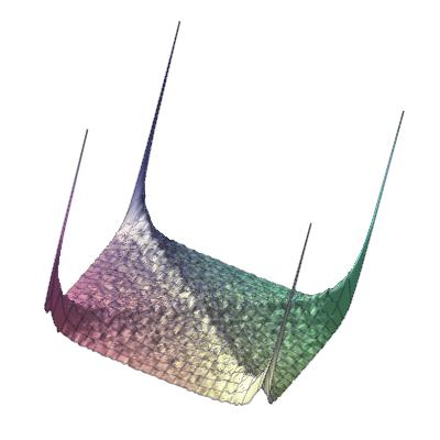
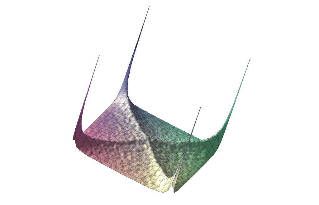
Figure 4. The shape of separable permutations (left), and of permutations taken in the substitution-closed class whose set of simple permutations is $\{2413,3142,24153\}$ (right).

Figure 4 shows average diagrams of permutations in the (substitution-closed) class $Av(2413,3142)$ of separable permutations, and in another substitution-closed class. These diagrams are obtained overlapping the diagrams of $10\,000$ permutations of size $100$ (resp. $500$). The representation is however a little different from Figure 3: in these 3D representations, for a point at coordinates $(x,y,z)$, $z$ is the number of permutations such that $\sigma(x)=y$. Leaving aside the difference in the representation, these figures suggest a very different limit behavior in substitution-closed and not substitution-closed classes.

Looking at these diagrams, a natural question is then to describe the average shape of permutations in classes. This is a question which has received quite a lot of attention lately, especially for classes $Av(\tau)$ for $\tau$ of size $3$, see [AM14, HRS14, MP14a, MP14b]. Inspired by Figure 4, some of us (in collaboration with V. Féray and L. Gerin) have described the limit shape of separable permutations in [BBFGP16], thus explaining the first diagram of Figure 4. As we discuss in [BBFGP16], we are working on generalizing this result to substitution-closed classes, which would also explain the second diagram of Figure 4.

3.3. Perspectives

As described in Section 3.2, our main result combines with previous works to yield an algorithm that produces, for any class $Av(B)$ containing finitely many simple permutations, a recursive (resp. Boltzmann) uniform random sampler. When generating permutations with such samplers, complexity is measured w.r.t. the size of the permutation produced and is quasilinear (resp. quadratic but can be made linear using classical tricks and allowing a small variation on the size of the output permutation [DFLS04]). However, the complexity is not at all measured w.r.t. the number of equations in the specification nor w.r.t. the number of terms in each equation. In our context, where the specifications are produced automatically, and potentially contain a large number of equations/terms, this dependency is of course relevant, and opens a new direction in the study of random samplers.

In addition to providing inspiration for the study of random permutations, our algorithmic chain has other applications. Indeed, the specifications obtained could also be used to compute or estimate growth rates of permutation classes. Moreover, the computed specifications could possibly be used to provide more efficient algorithms to test membership of a permutation to a class.

We should also mention that our procedure fails to be completely general. Although the method is generic and algorithmic, the classes that are fully handled by the algorithmic process are those containing a finite number of simple permutations. From [AA05], such classes are finitely based. And since there are countably many such permutation classes, only a very small subset of the (uncountably many) permutation classes is covered by our method.

But note that even if a class $\mathcal{C}$ contains an infinite number of simple permutations, we can (at least in theory) use our approach to perform random generation of permutations of the class $\mathcal{C}$. More precisely, fixing the maximum size $n$ of permutations we want to generate, we can apply our algorithm to a class $\mathcal{C}^{\prime}\subseteq\mathcal{C}$ containing finitely many simple permutations and that coincides with $\mathcal{C}$ up to size $n$. It is enough to choose $\mathcal{C}^{\prime}$ which is the subclass of $\mathcal{C}$ whose set of simple permutations consists in all simple permutations of $\mathcal{C}$ of size at most $n$, whose computation is explained in [PR12]. If the maximal size $n$ is large and if $\mathcal{C}$ has many simple permutations of each size, it is likely that the complexity of our algorithm will be too large for it to be of any use. But this approach may be relevant when the class has an infinite number of simple permutations, but a small number of each size.

To enlarge the framework of application of our algorithm computing specifications, we could explore the possibility of extending it to permutation classes that contain an infinite number of simple permutations, but that are finitely described. A family of such classes is considered in [ARV15], where the finite basis and algebraicity results of [AA05] are extended from classes with finitely many simple permutations to subclasses of substitution closures of geometrically griddable classes (we refer the reader to [ARV15] for definitions). The proofs in [ARV15] involve similar techniques as in [BHV08] (including query-complete sets), but not only. In particular, they heavily rely on the results of [AABRV13], which are non-constructive. Making all the process in [AABRV13] and [ARV15] constructive, and then turning it into an effective procedure, it may be possible to extend our algorithms to all classes considered in [ARV15]. But this is far from straightforward, and beyond the scope of the present work. Note that, with such an improvement, more classes would enter our framework, but it would be hard to leave the algebraic case.

4. Combinatorial specification of substitution-closed classes

In this section, we recall how to obtain a combinatorial specification for substitution-closed classes having finitely many simple permutations.

Recall that we denote by ${\hat{\mathcal{C}}}$ the substitution closure of the permutation class $\mathcal{C}$, and that $\mathcal{C}$ is substitution-closed when $\mathcal{C}={\hat{\mathcal{C}}}$, or equivalently when the permutations in $\mathcal{C}$ are exactly the ones whose decomposition trees have internal nodes labeled by $\oplus,\ominus$ or any simple permutation of $\mathcal{C}$.

For the purpose of this article, we additionally introduce the following notation:

Definition 4.1.

For any set $\mathcal{A}$ of permutations, $\mathcal{A}^{+}$ (resp. $\mathcal{A}^{-}$) denotes the set of permutations of $\mathcal{A}$ that are $\oplus$-indecomposable (resp. $\ominus$-indecomposable) and $\mathcal{S_{\mathcal{A}}}$ denotes the set of simple permutations of $\mathcal{A}$.

Theorem 2.11 (p.2.11) directly yields the following proposition:

Proposition 4.2 (Lemma 11 of [AA05]).

Let $\mathcal{C}={\hat{\mathcal{C}}}$ be a substitution-closed class. Then ${\hat{\mathcal{C}}}$ satisfies the following system of equations, denoted $\mathcal{E}_{{\hat{\mathcal{C}}}}$:

(1) $${\hat{\mathcal{C}}} = 1\ \uplus\ \oplus[{\hat{\mathcal{C}}}^{+},{\hat{\mathcal{C}}}]\ \uplus\ \ominus[{\hat{\mathcal{C}}}^{-},{\hat{\mathcal{C}}}]\ \textstyle\uplus\biguplus_{\pi\in{\mathcal{S}}_{\mathcal{C}}}\pi[{\hat{\mathcal{C}}},\dots,{\hat{\mathcal{C}}}]$$

(2) $${\hat{\mathcal{C}}}^{+} = 1\ \uplus\ \ominus[{\hat{\mathcal{C}}}^{-},{\hat{\mathcal{C}}}]\ \uplus\ \textstyle\biguplus_{\pi\in{\mathcal{S}}_{\mathcal{C}}}\pi[{\hat{\mathcal{C}}},\dots,{\hat{\mathcal{C}}}]$$

(3) $${\hat{\mathcal{C}}}^{-} = 1\ \uplus\ \oplus[{\hat{\mathcal{C}}}^{+},{\hat{\mathcal{C}}}]\ \uplus\ \textstyle\biguplus_{\pi\in{\mathcal{S}}_{\mathcal{C}}}\pi[{\hat{\mathcal{C}}},\dots,{\hat{\mathcal{C}}}].$$

Note that by Remark 2.16, ${\mathcal{S}}_{\mathcal{C}}={\mathcal{S}}_{\hat{\mathcal{C}}}$. By uniqueness of the substitution decomposition, unions are disjoint and so Equations (1) to (3) describe unambiguously the substitution-closed class ${\hat{\mathcal{C}}}$. Hence, Proposition 4.2 can be transposed in the framework of constructible structures as follows:

Theorem 4.3.

Let $\mathcal{C}$ be a substitution-closed class. Then $\mathcal{C}$ can be described as a constructible combinatorial class in the sense of Section 2.3 with the following combinatorial specification, where the $\mathcal{E}_{\pi}$ for $\pi$ in $\mathcal{S_{C}}$ are distinct objects of size $0$:

$$\begin{cases}\mathcal{C}=\mathcal{Z}+\ \mathcal{E}_{\oplus}\times\mathcal{C}^{+}\times\mathcal{C}\ +\ \mathcal{E}_{\ominus}\times\mathcal{C}^{-}\times\mathcal{C}\ +\ \sum_{\pi\in\mathcal{S_{C}}}\mathcal{E}_{\pi}\times\underbrace{\mathcal{C}\times\dotsb\times\mathcal{C}}_{|\pi|}\\ \mathcal{C}^{+}=\mathcal{Z}+\ \mathcal{E}_{\ominus}\times\mathcal{C}^{-}\times\mathcal{C}\ +\ \sum_{\pi\in\mathcal{S_{C}}}\mathcal{E}_{\pi}\times\underbrace{\mathcal{C}\times\dotsb\times\mathcal{C}}_{|\pi|}\\ \mathcal{C}^{-}=\mathcal{Z}+\ \mathcal{E}_{\oplus}\times\mathcal{C}^{+}\times\mathcal{C}\ +\ \sum_{\pi\in\mathcal{S_{C}}}\mathcal{E}_{\pi}\times\underbrace{\mathcal{C}\times\dotsb\times\mathcal{C}}_{|\pi|}.\end{cases}$$

Moreover this system can be translated into an equation for the generating function $C(z)$:

Proposition 4.4 (Theorem 12 of [AA05]).

Let $\mathcal{C}$ be a substitution-closed class, with generating function $C(z)$. Then

$$C(z)^{2}+(S_{\mathcal{C}}(C(z))-1+z)C(z)+S_{\mathcal{C}}(C(z))+z=0$$

with $S_{\mathcal{C}}(z)$ denoting the generating function that enumerate simple permutations in $\mathcal{C}$, i.e. $S_{\mathcal{C}}(z)=\sum_{\pi\in\mathcal{S_{C}}}z^{|\pi|}$.

Hence, in the case of a substitution-closed class $\mathcal{C}$ (and for the substitution closure ${\hat{\mathcal{C}}}$ of any class), the system $\mathcal{E}_{{\hat{\mathcal{C}}}}$ that recursively describes the permutations in ${\hat{\mathcal{C}}}$ can be immediately deduced from the set $\mathcal{S_{C}}$ of simple permutations in $\mathcal{C}$. As soon as $\mathcal{S_{C}}$ is finite and known, this system is explicit and gives a combinatorial specification.

Our next goal is to describe an algorithm that computes a combinatorial system of equations for a general permutation class $\mathcal{C}$ from the simple permutations in $\mathcal{C}$, like for the case of substitution-closed classes. However, when the class is not substitution-closed, this is not as straightforward as what we have seen in Proposition 4.2, and we provide details on how to solve this general case in the following sections.

5. A possibly ambiguous combinatorial system for permutation classes

In this section, we explain how to derive a system of equations for a class $\mathcal{C}$ with finitely many simple permutations from the combinatorial specification of its substitution closure. Our method follows the guideline of the constructive proof of [AA05, Theorem 10]. However, unlike [AA05], we make the whole process fully algorithmic.

The key idea of the method is to describe recursively the permutations in $\mathcal{C}$, replacing the constraint of avoiding the elements of the basis by constraints in the subtrees of the decomposition tree of permutations in $\mathcal{C}$. This is done by computing the embeddings of non-simple permutations $\gamma$ of the basis $B$ of $\mathcal{C}$ into simple permutations $\pi$ belonging to the class $\mathcal{C}$ (and into $\oplus$ and $\ominus$). These embeddings are block decompositions of the permutations $\gamma$, each (normalized) block being translated into a new avoidance constraint pushed downwards in the decomposition tree. We then need to add new equations in the specification for $\mathcal{C}$ to take into account these new constraints.

The main algorithm of this section is AmbiguousSystem (Algo. 1 below), which uses auxiliary procedures described later on. We prove in Section 5.4 that the result it produces has the following properties:

Theorem 5.1.

Let $\mathcal{C}$ be a permutation class with a finite number of simple permutations. Denote by $B$ the (finite) basis of $\mathcal{C}$, by ${B^{\star}}$ the subset of non-simple permutations in $B$, by ${\mathcal{S}}_{\mathcal{C}}$ the (finite) set of simple permutations in $\mathcal{C}$, and by $\mathcal{A}\langle E\rangle$ the set of permutations of a set $\mathcal{A}$ that avoid every pattern in a set $E$. The result of AmbiguousSystem$(B,{\mathcal{S}}_{\mathcal{C}})$ is a finite system of combinatorial equations describing $\mathcal{C}$. The equations of this system are all of the form ${\mathcal{D}}_{0}=1\ \cup\ \bigcup\pi[{\mathcal{D}}_{1},\dots,{\mathcal{D}}_{n}]$, where ${\mathcal{D}}_{i}={\hat{\mathcal{C}}}^{\delta}\langle{B^{\star}}\cup B_{i}\rangle$ with $\delta\in\{~{},+,-\}$ and $B_{i}$ contains only permutations corresponding to normalized blocks of elements of ${B^{\star}}$. This system contains an equation whose left part is $\mathcal{C}$ and is complete, that is: every ${\mathcal{D}}_{i}$ that appears in the system is the left part of one equation of the system.

Data: A finite basis of forbidden patterns defining ${\mathcal{C}}=Av(B)$ and the finite set $\mathcal{S}_{\mathcal{C}}$ of simple permutations in $\mathcal{C}$.

Result: A system of equations of the form ${\mathcal{D}}_{0}=1\cup\bigcup\pi[{\mathcal{D}}_{1},\dots,{\mathcal{D}}_{n}]$ defining $\mathcal{C}$.

begin

       $\mathcal{E}\leftarrow$ EqnForClass$({\hat{\mathcal{C}}},{B^{\star}})$

        /* See Algo. 5 (p.5) */

       while there is a right-only ${\hat{\mathcal{C}}}^{\delta}\langle E\rangle$ in some equation of $\mathcal{E}$ do

             $\mathcal{E}\leftarrow\mathcal{E}~{}\cup$ EqnForClass(${\hat{\mathcal{C}}}^{\delta}$, $E$)

      

Algorithm 1 AmbiguousSystem($B,{\mathcal{S}}_{\mathcal{C}}$)

An essential remark is that the obtained combinatorial system may be ambiguous, since it may involve unions of sets that are not always disjoint. We will tackle the problem of computing a non-ambiguous system in Section 6.

It is also to note that the result of AmbiguousSystem provides a finite query-complete set containing $\mathcal{C}$:

Corollary 5.2.

Let ${\mathcal{E}}$ be the system of equations output by AmbiguousSystem$(B,{\mathcal{S}}_{\mathcal{C}})$. Then the set $\{{\mathcal{D}}:{\mathcal{D}}\text{ is the left part of some equation of }{\mathcal{E}}\}$ is a query-complete set containing $\mathcal{C}$.

Proof.

This a direct consequence of the form of ${\mathcal{E}}$ described in Theorem 5.1. ∎

5.1. A first system of equations

Consider a permutation class ${\mathcal{C}}$, whose basis is $B$ and which is not substitution-closed. We compute a system describing $\mathcal{C}$ by adding constraints to the system obtained for ${\hat{\mathcal{C}}}$, as in [AA05]. We denote by ${B^{\star}}$ the subset of non-simple permutations of $B$ and by $\mathcal{A}\langle E\rangle$ the set of permutations of $\mathcal{A}$ that avoid every pattern in $E$, for any set $\mathcal{A}$ of permutations and any set $E$ of patterns. Note that we have $(\mathcal{A}\langle E\rangle)^{+}=\mathcal{A}^{+}\langle E\rangle$: the corresponding set is the one of permutations of $\mathcal{A}$ that avoid $E$ and that are $\oplus$-indecomposable. The same goes for $\mathcal{A}^{-}$.

Proposition 5.3.

Let $\mathcal{C}$ be a permutation class, that contains $12$ and $21$. We have that $\mathcal{C}^{\delta}={\hat{\mathcal{C}}}^{\delta}\langle{B^{\star}}\rangle$ for $\delta\in\{~{},+,-\}$. Moreover,

(4) $${\hat{\mathcal{C}}}\langle{B^{\star}}\rangle = 1\ \uplus\ \oplus[{\hat{\mathcal{C}}}^{+},{\hat{\mathcal{C}}}]\langle{B^{\star}}\rangle\ \uplus\ \ominus[{\hat{\mathcal{C}}}^{-},{\hat{\mathcal{C}}}]\langle{B^{\star}}\rangle\ \uplus\textstyle\biguplus_{\pi\in{\mathcal{S}}_{\mathcal{C}}}\pi[{\hat{\mathcal{C}}},\dots,{\hat{\mathcal{C}}}]\langle{B^{\star}}\rangle$$

(5) $${\hat{\mathcal{C}}}^{+}\langle{B^{\star}}\rangle = 1\ \uplus\ \ominus[{\hat{\mathcal{C}}}^{-},{\hat{\mathcal{C}}}]\langle{B^{\star}}\rangle\ \uplus\ \textstyle\biguplus_{\pi\in{\mathcal{S}}_{\mathcal{C}}}\pi[{\hat{\mathcal{C}}},\dots,{\hat{\mathcal{C}}}]\langle{B^{\star}}\rangle$$

(6) $${\hat{\mathcal{C}}}^{-}\langle{B^{\star}}\rangle = 1\ \uplus\ \oplus[{\hat{\mathcal{C}}}^{+},{\hat{\mathcal{C}}}]\langle{B^{\star}}\rangle\ \uplus\ \textstyle\biguplus_{\pi\in{\mathcal{S}}_{\mathcal{C}}}\pi[{\hat{\mathcal{C}}},\dots,{\hat{\mathcal{C}}}]\langle{B^{\star}}\rangle,$$

all these unions being disjoint.

Proof.

Let $\sigma\in\mathcal{C}$, then $\sigma\in{\hat{\mathcal{C}}}$ and $\sigma$ avoids ${B^{\star}}$, thus $\sigma\in{\hat{\mathcal{C}}}\langle{B^{\star}}\rangle$. Conversely, let $\sigma\in{\hat{\mathcal{C}}}\langle{B^{\star}}\rangle$ and let $\pi\in B$. If $\pi\in{B^{\star}}$ then $\sigma$ avoids $\pi$. Otherwise, $\pi$ is simple and $\pi\notin\mathcal{C}$. Because ${\mathcal{S}}_{\hat{\mathcal{C}}}={\mathcal{S}}_{\mathcal{C}}$ by Remark 2.16, this implies that $\pi\notin{\hat{\mathcal{C}}}$. Since $\sigma\in{\hat{\mathcal{C}}}$, $\sigma$ avoids $\pi$. Hence $\sigma\in\mathcal{C}$. Finally ${\hat{\mathcal{C}}}\langle{B^{\star}}\rangle=\mathcal{C}$, thus ${\hat{\mathcal{C}}}^{\delta}\langle{B^{\star}}\rangle=\mathcal{C}^{\delta}$. Then the result follows from Proposition 4.2. ∎

Equations (4) to (6) do not provide a combinatorial specification because the terms $\pi[{\hat{\mathcal{C}}},\dots,{\hat{\mathcal{C}}}]\langle{B^{\star}}\rangle$ are not simply expressed from the terms appearing on the left-hand side of these equations. To solve this problem, instead of decorating all terms on the right-hand side of Equations (1)–(3) with constraint $\langle{B^{\star}}\rangle$ (like in Equations (4)–(6)), we propagate the constraint $\langle{B^{\star}}\rangle$ into the subtrees. More precisely, by Lemma 18 of [AA05], sets $\pi[{\hat{\mathcal{C}}},\dots,{\hat{\mathcal{C}}}]\langle{B^{\star}}\rangle$ can be expressed as union of smaller sets:

(7) $$\pi[{\hat{\mathcal{C}}},\dots,{\hat{\mathcal{C}}}]\langle{B^{\star}}\rangle=\textstyle\bigcup_{i=1}^{\ell}\pi[{\hat{\mathcal{C}}}\langle E_{i,1}\rangle,{\hat{\mathcal{C}}}\langle E_{i,2}\rangle,\ldots,{\hat{\mathcal{C}}}\langle E_{i,k}\rangle]$$

where the $E_{i,j}$ are sets of permutations which are patterns of some permutations of ${B^{\star}}$. For instance, with $\mathcal{C}=Av(231)$, we have ${B^{\star}}=\{231\}$, and $\ominus[{\hat{\mathcal{C}}}^{-},{\hat{\mathcal{C}}}]\langle 231\rangle=\ominus[{\hat{\mathcal{C}}}^{-}\langle 12\rangle,{\hat{\mathcal{C}}}\langle 231\rangle]$. Note that the set ${\hat{\mathcal{C}}}^{-}\langle 12\rangle$, which is not a part of the initial system, has appeared on the right-hand side of this equation, and we now need a new equation to describe it. In the general case, applying Equation (7) in the system of Proposition 5.3 introduces sets of the form ${\hat{\mathcal{C}}}^{\delta}\langle E_{i,j}\rangle$ on the right-hand side of an equation of the system that do not appear on the left-hand side of any equation. The reason is that $\{\mathcal{C},\mathcal{C}^{+},\mathcal{C}^{-}\}$ is not query-complete in general. Propagating the constraints in the subtrees as described below allows to determine a query-complete set which contains $\mathcal{C}$ (see Corollary 5.2).

We call right-only sets the sets of the form ${\hat{\mathcal{C}}}^{\delta}\langle E_{i,j}\rangle$ which appear only on the right-hand side of an equation of the system. For each such set, we need to add a new equation to the system, starting from Equation (1), (2) or (3) depending on $\delta$, and propagating constraint $E_{i,j}$ instead of ${B^{\star}}$. This may create new right-only terms in these new equations, and they are treated recursively in the same way. This process terminates, since the $E_{i,j}$ are sets of patterns of elements of ${B^{\star}}$, and there is only a finite number of such sets (as $B$ is finite).

The key to the precise description of the sets $E_{i,j}$, and to their effective computation, is given by the embeddings of permutations $\gamma$ that are patterns of some $\beta\in{B^{\star}}$ into the simple permutations $\pi$ of $\mathcal{C}$.

5.2. Embeddings: definition and computation

Recall that $\varepsilon$ denotes the empty permutation, i.e. the permutation of size $0$. We take the convention $\mathcal{A}\langle\varepsilon\rangle=\emptyset$.

A generalized substitution (also called lenient inflation in [BHV08]) $\sigma\{\pi^{1},\pi^{2},\ldots,\pi^{n}\}$ is defined like a substitution with the particularity that any $\pi^{i}$ may be the empty permutation. Note that $\sigma[\pi^{1},\pi^{2},\ldots,\pi^{n}]$ necessarily contains $\sigma$ whereas $\sigma\{\pi^{1},\pi^{2},\ldots,\pi^{n}\}$ may avoid $\sigma$. For instance, the generalized substitution $1\,3\,2\{2\,1,\varepsilon,1\}$ gives the permutation $2\,1\,3$ which avoids $1\,3\,2$.

Thanks to generalized substitutions, we define the notion of embedding, which expresses how a pattern $\gamma$ can be involved in a permutation whose decomposition tree has a root $\pi$:

Definition 5.4.

Let $\pi=\pi_{1}\dots\pi_{n}$ and $\gamma$ be two permutations of size $n$ and $p$ respectively and $P_{\gamma}$ the set of intervals of $\gamma$, including the trivial ones. An embedding of $\gamma$ in ${\pi=\pi_{1}\dots\pi_{n}}$ is a map $\alpha$ from $\{1,\ldots,n\}$ to $P_{\gamma}$ such that:

• if the intervals $\alpha(i)$ and $\alpha(j)$ are not empty, and $i<j$, then $\alpha(i)$ consists of smaller indices than $\alpha(j)$;

• as a word, $\alpha(1)\ldots\alpha(n)$ is a factorization of the word $1\ldots|\gamma|$ (which may include empty factors).

• it holds that $\pi\{\gamma_{\alpha(1)},\dots,\gamma_{\alpha(n)}\}=\gamma$ (see Definition 2.1 (p.2.1) for the definition of $\gamma_{\alpha(i)}$).

Example 5.5.

For any permutations $\gamma$ and $\pi$, $\alpha:\begin{cases}1&\mapsto[1..|\gamma|]\\ k>1&\mapsto\emptyset\end{cases}$ is an embedding of $\gamma$ in $\pi$. Indeed $\gamma_{[1..|\gamma|]}=\gamma$ and $\pi\{\gamma,\varepsilon,\dots,\varepsilon\}=\gamma$.

Note that if we denote the non-empty images of $\alpha$ by $\alpha^{1},\dots,\alpha^{N}$ and if we remove from $\pi$ the $\pi_{i}$ such that $\alpha(i)=\varepsilon$, we obtain a pattern $\sigma$ of $\pi$ such that $\gamma=\sigma[\gamma_{\alpha^{1}},\dots,\gamma_{\alpha^{N}}]$. But this pattern $\sigma$ may occur at several places in $\pi$ so a block decomposition $\gamma=\sigma[\gamma_{\alpha^{1}},\dots,\gamma_{\alpha^{N}}]$ may correspond to several embeddings of $\gamma$ in $\pi$.

Example 5.6.

There are $12$ embeddings of $\gamma=5\,4\,6\,3\,1\,2$ into $\pi=3\,1\,4\,2$, shown in Table 1. For instance, when writing $\gamma$ as the substitution ${\ominus[3241,12]}$, they are derived from the generalized substitutions $\pi\{3241,12,\varepsilon,\varepsilon\}$, $\pi\{3241,\varepsilon,\varepsilon,12\}$ and $\pi\{\varepsilon,\varepsilon,3241,12\}$, corresponding to the three occurrences of $21$ in $\pi$. But when writing $\gamma$ as $312[3241,1,1]$, since $312$ has only one occurrence in $\pi$, only one embedding is derived, which comes from $\pi\{3241,1,\varepsilon,1\}$.

		$\gamma_{\alpha(1)}$	$\gamma_{\alpha(2)}$	$\gamma_{\alpha(3)}$	$\gamma_{\alpha(4)}$
$\gamma=1[546312]$	$=\pi\{546312,\varepsilon,\varepsilon,\varepsilon\}$	$546312$	$\varepsilon$	$\varepsilon$	$\varepsilon$
	$=\pi\{\varepsilon,546312,\varepsilon,\varepsilon\}$	$\varepsilon$	$546312$	$\varepsilon$	$\varepsilon$
	$=\pi\{\varepsilon,\varepsilon,546312,\varepsilon\}$	$\varepsilon$	$\varepsilon$	$546312$	$\varepsilon$
	$=\pi\{\varepsilon,\varepsilon,\varepsilon,546312\}$	$\varepsilon$	$\varepsilon$	$\varepsilon$	$546312$
$\gamma=\ominus[213,312]$	$=\pi\{213,312,\varepsilon,\varepsilon\}$	$213$	$312$	$\varepsilon$	$\varepsilon$
	$=\pi\{213,\varepsilon,\varepsilon,312\}$	$213$	$\varepsilon$	$\varepsilon$	$312$
	$=\pi\{\varepsilon,\varepsilon,213,312\}$	$\varepsilon$	$\varepsilon$	$213$	$312$
$\gamma=\ominus[3241,12]$	$=\pi\{3241,12,\varepsilon,\varepsilon\}$	$3241$	$12$	$\varepsilon$	$\varepsilon$
	$=\pi\{3241,\varepsilon,\varepsilon,12\}$	$3241$	$\varepsilon$	$\varepsilon$	$12$
	$=\pi\{\varepsilon,\varepsilon,3241,12\}$	$\varepsilon$	$\varepsilon$	$3241$	$12$
$\gamma=231[21,1,312]$	$=\pi\{21,\varepsilon,1,312\}$	$21$	$\varepsilon$	$1$	$312$
$\gamma=312[3241,1,1]$	$=\pi\{3241,1,\varepsilon,1\}$	$3241$	$1$	$\varepsilon$	$1$

Table 1. The embeddings of $\gamma=5\,4\,6\,3\,1\,2$ into $\pi=3\,1\,4\,2$.

Note that this definition of embeddings conveys the same notion as in [AA05], but it is formally different and it will turn out to be more adapted to the definition of the sets $E_{i,j}$ in Section 5.3.

For now, we present how to compute the embeddings of some permutation $\gamma$ into a permutation $\pi$. This is done with AllEmbeddings (Algo. 2) in two main steps, as suggested by the two parts of Table 1. First we compute all block decompositions of $\gamma$ (the left part of the table shows only some block decompositions of $\gamma=5\,4\,6\,3\,1\,2$, namely those that can be expressed as a generalized substitution in $\pi=3\,1\,4\,2$). Then for each block decomposition of $\gamma$, we compute all the embeddings of $\gamma$ into $\pi$ which correspond to this block decomposition (this is the right part of the table).

Data: Two permutations $\gamma$ and $\pi$

Result: The set of embeddings of $\gamma$ into $\pi$

begin

       $\mathcal{E}\leftarrow\emptyset$

       $\mathcal{D}\leftarrow$ BlockDecompositions$(\gamma)$

        /* See Algo. 3 */

       foreach $d\in\mathcal{D}$ do

            $\mathcal{E}\leftarrow\mathcal{E}\,\cup$ Embeddings$(d,\pi)$

              /* See Algo. 4 */

            

      return $\mathcal{E}$

      

Algorithm 2 AllEmbeddings$(\gamma,\pi)$

Data: A permutation $\gamma$

Result: The set $\mathcal{D}$ of block decompositions of $\gamma$

begin

       $\mathcal{D}\leftarrow\emptyset$;  $\mathcal{P}\leftarrow$ Intervals$(\gamma,1)$

       foreach $u=\Big{(}(i_{1},j_{1}),\dots,(i_{m},j_{m})\Big{)}\in\mathcal{P}$ do

            $\mathcal{P}\leftarrow\mathcal{P}\setminus\{u\}$

             if $j_{m}=|\gamma|$ then $\mathcal{D}\leftarrow\mathcal{D}\cup\{u\}$

             else

                  $\mathcal{S}\leftarrow$ Intervals$(\gamma,j_{m}+1)$

                   $\mathcal{P}\leftarrow\mathcal{P}\cup\{u\cdot s\mid s\in\mathcal{S}\}$

            

      return $\mathcal{D}$

      

/* Returns the set of intervals of $\gamma$ of the form $(i,j)$ */

Intervals $($$\gamma,i$

$($

       $\mathcal{I}\leftarrow\emptyset$

       $max\leftarrow\gamma_{i}$; $min\leftarrow\gamma_{i}$

       for $j$ from $i$ to $|\gamma|$ do

             $max\leftarrow\max(max,\gamma_{j})$; $min\leftarrow\min(min,\gamma_{j})$

             if $max-min=j-i$ then $\mathcal{I}\leftarrow\mathcal{I}\cup\{(i,j)\}$

            

      return $\mathcal{I}$

Algorithm 3 BlockDecompositions$(\gamma)$

The procedure BlockDecompositions (Algo. 3) finds all the block decompositions of $\gamma$. It needs to compute all the intervals of $\gamma$. Such intervals can be described as pairs of indices $(i,j)$ with $i\leq j$ such that $\max_{i\leq k\leq j}(\gamma_{k})-\min_{i\leq k\leq j}(\gamma_{k})=j-i$. Denoting by $p$ the size of $\gamma$, this remark allows to compute easily all the intervals starting at $i$, for each $i\in[1..p]$ – see Intervals$(\gamma,i)$. Then, BlockDecompositions builds the set $\mathcal{D}$ of all sequences of intervals of the form $\big{(}(i_{1},j_{1}),\dots,(i_{m},j_{m})\big{)}$ with $i_{1}=1$, $j_{m}=p$, and $i_{k+1}=j_{k}+1$ for all $k<m$. These sequences correspond exactly to the block decompositions of $\gamma$. They are computed iteratively, starting from all the intervals of the form $(1,i)$ and examining how they can be extended to a sequence of intervals in $\mathcal{D}$. To this end, note that any sequence $\big{(}(i_{1},j_{1}),\dots,(i_{m},j_{m})\big{)}$ as above but such that $j_{m}\neq p$ is the prefix of at least one sequence of $\mathcal{D}$, since for every $i\in[1..p]$, at least $(i,i)$ is an interval of $\gamma$.

For each $i\in[1..p]$, computing Intervals$(\gamma,i)$ is done in $\mathcal{O}(p)$, so $\mathcal{O}(p^{2})$ is enough to compute once and for all the results of Intervals$(\gamma,i)$ for all $i\in[1..p]$ (provided we store them). The computation of all block decompositions of $\gamma$ with BlockDecompositions$(\gamma)$ then costs $\mathcal{O}(p\,2^{p})$. Indeed there are at most $2^{p-1}$ such sequences of $\mathcal{D}$ and each sequence of $\mathcal{D}$ contains at most $p$ intervals. At each step, the algorithm extends a sequence already built. Thus the (amortized) overall complexity is $\mathcal{O}(p\,2^{p})$ and this bound is tight.

Data: A permutation $\pi$ of size $n$ and a block decomposition $d\in\mathcal{D}$ of $\gamma$, $d=\Big{(}(i_{1},j_{1}),\dots,(i_{m},j_{m})\Big{)}$

Result: The set of embeddings of $\gamma$ into $\pi$ which correspond to $d$

begin

       if $m>n$ then /* No embedding of $\gamma$ into $\pi$ corresponding to $d$ */

            return $\emptyset$

      else

             /* $\sigma$ is the skeleton such that $d=\sigma[\gamma^{(1)},\ldots,\gamma^{(m)}]$ */

             $\sigma\leftarrow$ $\gamma_{\{i_{1},i_{2},\ldots,i_{m}\}}$

             $\mathcal{E}\leftarrow\emptyset$

             foreach subset $S=\{s_{1},\ldots,s_{m}\}$ of $\{1,2,\ldots,n\}$ with $s_{1}<\ldots<s_{m}$ do

                  if $\pi_{\{s_{1},s_{2},\ldots,s_{m}\}}=\sigma$ then

                         $\alpha\leftarrow$ embedding of $\gamma$ in $\pi$ such that $\begin{cases}\alpha(s_{k})=[i_{k}..j_{k}]\text{ for }1\leq k\leq m\\ \alpha(i)=\varepsilon\text{ for }i\notin S\end{cases}$

                         $\mathcal{E}\leftarrow\mathcal{E}\cup\{\alpha\}$

                        

                  

            return $\mathcal{E}$

      

Algorithm 4 Embeddings$(d,\pi)$

The procedure Embeddings (Algo. 4) finds the embeddings of $\gamma$ in $\pi$ which correspond to a given block-decomposition of $\gamma$. The output $\mathcal{D}$ of BlockDecompositions corresponds to all the substitutions $\sigma[\gamma^{(1)},\ldots,\gamma^{(m)}]$ which are equal to $\gamma$. For each $d\in\mathcal{D}$ we first determine the corresponding skeleton $\sigma$ defined as the normalization of a sequence $s_{1}\ldots s_{m}$ of $m$ integers, where each $s_{i}$ is an element of $\gamma$ falling into the $i$-th block of this decomposition. Then, we compute the set of occurrences of $\sigma$ in $\pi$, since they are in one-to-one correspondence with embeddings of $\gamma$ into $\pi$ which corresponds to the given substitution $\gamma=\sigma[\gamma^{(1)},\ldots,\gamma^{(m)}]$. These occurrences are naively computed by testing, for every subsequence of $m$ elements of $\pi$, whether it is an occurrence of $\sigma$.

The preprocessing part of Embeddings (Algo. 4), which consists in the computation of the skeleton $\sigma$, costs $\mathcal{O}(m)$. The examination of all possible occurrences of $\sigma$ in $\pi$ is then performed in $\mathcal{O}(m\,{\binom{n}{m}})$, where $n$ is the size of $\pi$.

In total, computing the set $\mathcal{D}$ of block decompositions of $\gamma$ is performed in $\mathcal{O}(p\,2^{p})$. The set $\mathcal{D}$ contains at most ${\binom{p-1}{m-1}}$ block decompositions in $m$ blocks, so that the complexity of the main loop of AllEmbeddings is at most $\sum_{m=1}^{p}m{\binom{n}{m}}{\binom{p-1}{m-1}}\leq p\,2^{n+p-1}$. Note that it can be reduced to $\min(p,n)\,2^{n+\min(p,n)-1}$, by discarding all block decompositions of $\gamma$ in $m>n$ blocks, since these will never be used in an embedding of $\gamma$ into $\pi$. The upper bound $\sum_{m=1}^{p}m{\binom{n}{m}}{\binom{p-1}{m-1}}$ is tight, as can be seen with $p\leq n$, $\gamma=12\ldots p$ and $\pi=12\ldots n$.

In the next section, we explain how to use embeddings to propagate the pattern avoidance constraints in the subtrees.

5.3. Propagating constraints

To compute our combinatorial system, we compute equations for sets ${\hat{\mathcal{C}}}^{\delta}\langle E\rangle$ (initially for ${\hat{\mathcal{C}}}\langle{B^{\star}}\rangle$, that is $\mathcal{C}$) starting from Equation (1), (2) or (3) (p.1). For every set $\pi[{\hat{\mathcal{C}}}_{1},\dots,{\hat{\mathcal{C}}}_{n}]$ that appears on the right-hand side of the equation, we push the pattern avoidance constraints of $E$ in the subtrees. This is achieved using embeddings of excluded patterns in the root $\pi$. For instance, assume that $\gamma=5\,4\,6\,3\,1\,2\in B^{\star}$ and $\mathcal{S}_{\mathcal{C}}=\{3142\}$, and consider $3142[{\hat{\mathcal{C}}},{\hat{\mathcal{C}}},{\hat{\mathcal{C}}},{\hat{\mathcal{C}}}]\langle\gamma\rangle$. The embeddings of $\gamma$ in $3142$ indicates how the pattern $\gamma$ can be found in the subtrees in $3142[{\hat{\mathcal{C}}},{\hat{\mathcal{C}}},{\hat{\mathcal{C}}},{\hat{\mathcal{C}}}]$. The first embedding of Example 5.6 indicates that the full pattern $\gamma$ can appear all included in the first subtree. On the other hand, the last embedding of the same example tells us that $\gamma$ can spread over all the subtrees of $3142$ except the third one. In order to avoid this particular embedding of $\gamma$, it is enough to avoid one of the induced pattern $\gamma_{I}$ in one of the subtrees. However, in order to ensure that $\gamma$ is avoided, the constraints resulting from all the embeddings must be considered and merged. This is formalized in Proposition 5.7.

Proposition 5.7.

Let $\pi$ be a simple permutation of size $n$ and $\mathcal{C}_{1},\dots,\mathcal{C}_{n}$ be sets of permutations. For any permutation $\gamma$, the set $\pi[\mathcal{C}_{1},\dots,\mathcal{C}_{n}]\langle\gamma\rangle$ rewrites as a union of sets of the form $\pi[{\mathcal{D}}_{1},\dots,{\mathcal{D}}_{n}]$ where, for all $i$, ${\mathcal{D}}_{i}=\mathcal{C}_{i}\langle\gamma,\dots\rangle$ and the restrictions appearing after $\gamma$ (if there are any) are patterns of $\gamma$ corresponding to normalized blocks of $\gamma$.

More precisely, we have

(8) $$\pi[\mathcal{C}_{1},\dots,\mathcal{C}_{n}]\langle\gamma\rangle=\bigcup_{(k_{1},\dots,k_{\ell})\in K^{\pi}_{\gamma}}\pi[\mathcal{C}_{1}\langle E_{1,k_{1}\dots k_{\ell}}\rangle,\dots,\mathcal{C}_{n}\langle E_{n,k_{1}\dots k_{\ell}}\rangle]$$

where $K^{\pi}_{\gamma}=\{(k_{1},\dots,k_{\ell})\in[1..n]^{\ell}\ |\ \forall i,\ \gamma_{\alpha_{i}(k_{i})}\neq\varepsilon\text{ and }\gamma_{\alpha_{i}(k_{i})}\neq 1\}$ and $E_{m,k_{1}\dots k_{\ell}}=\{\gamma_{\alpha_{i}(k_{i})}\ |\ i\in[1..\ell]\text{ and }k_{i}=m\}$, $\{\alpha_{1},\dots,\alpha_{\ell}\}$ being the set of embeddings of $\gamma$ in $\pi$.

Similarly, $\oplus[\mathcal{C}^{+}_{1},\mathcal{C}_{2}]\langle\gamma\rangle$ (resp. $\ominus[\mathcal{C}^{-}_{1},\mathcal{C}_{2}]\langle\gamma\rangle$) rewrites as the union over $K^{12}_{\gamma}$ (resp. $K^{21}_{\gamma}$) of sets $\oplus[{\mathcal{D}}_{1}^{+},{\mathcal{D}}_{2}]$ (resp. $\ominus[{\mathcal{D}}_{1}^{-},{\mathcal{D}}_{2}]$) with ${\mathcal{D}}_{i}=\mathcal{C}_{i}\langle E_{i,k_{1}\dots k_{\ell}}\rangle$.

Proposition 5.7 and its proof heavily borrow from the proof of Lemma 18 of [AA05]. There are however several differences.

In the first part of our statement, while we stop at the condition ${\mathcal{D}}_{i}=\mathcal{C}_{i}\langle\gamma,\dots\rangle$ (which appears in the proof of Lemma 18 in [AA05]), [AA05] rephrases it as: ${\mathcal{D}}_{i}$ is $\mathcal{C}_{i}\langle\gamma\rangle$ or a strong subclass of this class (that is, a proper subclass of $\mathcal{C}_{i}$ which has the property that every basis element of ${\mathcal{D}}_{i}$ is involved in some basis element of $\mathcal{C}_{i}$). Note that this rephrasing is not always correct (but this does not affect the correctness of the result of [AA05] which uses their Lemma 18). A counter example is obtained taking $\pi=2413$, $\mathcal{C}_{i}=Av(12)$ for all $i$ and $\gamma=2143$. Then, because of the embedding of $\gamma$ in $\pi$ that maps $21$ in $\pi_{1}$ and $43$ in $\pi_{2}$, we get a term with ${\mathcal{D}}_{1}=\mathcal{C}_{1}\langle 2143,21\rangle=Av(12,21)$, which is not a strong subclass of $\mathcal{C}_{1}\langle\gamma\rangle=Av(12)$.

The second part of Proposition 5.7 is not present in [AA05]. That is, Proposition 5.7 goes further than the proof of Lemma 18 of [AA05]: we provide a statement which is nonetheless constructive as the proof of [AA05], but also explicit, so that it can be directly used for algorithmic purpose.

Proof.

We first consider the case of a simple root $\pi$. Let $\gamma$ be a permutation and $\{\alpha_{1},\dots,\alpha_{\ell}\}$ be the set of embeddings of $\gamma$ in $\pi$, each $\alpha_{i}$ being associated to the generalized substitution $\gamma=\pi\{\gamma_{\alpha_{i}(1)},\dots,\gamma_{\alpha_{i}(n)}\}$.

Let $\sigma=\pi[\sigma^{(1)},\dots,\sigma^{(n)}]$ where each $\sigma^{(k)}\in\mathcal{C}_{k}$. Then $\sigma$ avoids $\gamma$ if and only if for every embedding $\alpha_{i}$ (with $1\leq i\leq\ell$), there exists $k_{i}\in[1..n]$ such that $\gamma_{\alpha_{i}(k_{i})}$ is not a pattern of $\sigma^{(k_{i})}$, i.e. such that $\sigma^{(k_{i})}$ avoids $\gamma_{\alpha_{i}(k_{i})}$. Equivalently, $\sigma$ avoids $\gamma$ if and only if there exists a tuple $(k_{1},\dots,k_{\ell})\in[1..n]^{\ell}$ such that for every embedding $\alpha_{i}$ (with $1\leq i\leq\ell$), $\sigma^{(k_{i})}$ avoids $\gamma_{\alpha_{i}(k_{i})}$. Thus,

$$\pi[\mathcal{C}_{1},\dots,\mathcal{C}_{n}]\langle\gamma\rangle=\bigcup_{(k_{1},\dots,k_{\ell})\in[1..n]^{\ell}}\ \bigcap_{i=1}^{\ell}\pi[\mathcal{C}_{1},\dots,\mathcal{C}_{k_{i}}\langle\gamma_{\alpha_{i}(k_{i})}\rangle,\dots,\mathcal{C}_{n}].$$

But, for any set ${\mathcal{A}}$ of permutations we have ${\mathcal{A}}\langle\varepsilon\rangle=\emptyset$. So if for some $i\in[1..\ell]$, $\gamma_{\alpha_{i}(k_{i})}=\varepsilon$, then $\bigcap_{i=1}^{\ell}\pi[\mathcal{C}_{1},\dots,\mathcal{C}_{k_{i}}\langle\gamma_{\alpha_{i}(k_{i})}\rangle,\dots,\mathcal{C}_{n}]=\emptyset$. The same goes for the trivial permutation $1$ since every permutation contains $1$.
Therefore, we have:

$$\pi[\mathcal{C}_{1},\dots,\mathcal{C}_{n}]\langle\gamma\rangle=\bigcup_{(k_{1},\dots,k_{\ell})\in K^{\pi}_{\gamma}}\ \bigcap_{i=1}^{\ell}\pi[\mathcal{C}_{1},\dots,\mathcal{C}_{k_{i}}\langle\gamma_{\alpha_{i}(k_{i})}\rangle,\dots,\mathcal{C}_{n}],$$

with $K^{\pi}_{\gamma}=\{(k_{1},\dots,k_{\ell})\in[1..n]^{\ell}\ |\ \forall i,\ \gamma_{\alpha_{i}(k_{i})}\neq\varepsilon\text{ and }\gamma_{\alpha_{i}(k_{i})}\neq 1\}$. Following Example 5.6, and denoting $\alpha_{1}$ to $\alpha_{12}$ the embeddings of Table 1 from top to bottom, we have for example $\mathbf{k}=(1,2,3,4,1,4,4,2,1,4,4,1)\in K^{\pi}_{\gamma}$.

Moreover, as $\pi$ is simple, by uniqueness of the substitution decomposition we have for any sets of permutations $E_{1},\dots,E_{n},$ $F_{1},\dots,F_{n}$:

$$\pi[\mathcal{C}_{1}\langle E_{1}\rangle,\dots,\mathcal{C}_{n}\langle E_{n}\rangle]\cap\pi[\mathcal{C}_{1}\langle F_{1}\rangle,\dots,\mathcal{C}_{n}\langle F_{n}\rangle]=\pi[\mathcal{C}_{1}\langle E_{1}\cup F_{1}\rangle,\dots,\mathcal{C}_{n}\langle E_{n}\cup F_{n}\rangle].$$

Thus,

$$\pi[\mathcal{C}_{1},\dots,\mathcal{C}_{n}]\langle\gamma\rangle=\bigcup_{(k_{1},\dots,k_{\ell})\in K^{\pi}_{\gamma}}\pi[\mathcal{C}_{1}\langle E_{1,k_{1}\dots k_{\ell}}\rangle,\dots,\mathcal{C}_{n}\langle E_{n,k_{1}\dots k_{\ell}}\rangle].$$

where $E_{m,k_{1}\dots k_{\ell}}=\{\gamma_{\alpha_{i}(k_{i})}\ |\ i\in[1..\ell]\text{ and }k_{i}=m\}$. Following the same example again, $E_{1,\mathbf{k}}=\{\gamma_{\alpha_{1}(1)},\gamma_{\alpha_{5}(1)},\gamma_{\alpha_{9}(1)},\gamma_{\alpha_{12}(1)}\}=\{546312,213,3241\}$, $E_{2,\mathbf{k}}=\{546312,12\}$, $E_{3,\mathbf{k}}=\{546312\}$ and $E_{4,\mathbf{k}}=\{546312,312,12\}$.

Proposition 5.7 follows as soon as we ensure that each set $E_{m,k_{1}\dots k_{\ell}}$ contains $\gamma$ and possibly other restrictions that are patterns of $\gamma$ corresponding to normalized blocks of $\gamma$. For a given $m\in[1..n]$, there always exists an embedding of $\gamma$ in $\pi$ that maps the whole permutation $\gamma$ to $\pi_{m}$. Denoting this embedding $\alpha_{j_{m}}$, we have $\gamma_{\alpha_{j_{m}}(m)}=\gamma$ and $\gamma_{\alpha_{j_{m}}(q)}=\varepsilon$ for $q\neq m$. Consequently, if $k_{j_{m}}\neq m$ then $\gamma_{\alpha_{j_{m}}(k_{j_{m}})}=\varepsilon$ and $(k_{1},\dots,k_{\ell})\notin K^{\pi}_{\gamma}$. Therefore when $(k_{1},\dots,k_{\ell})\in K^{\pi}_{\gamma}$ then $k_{j_{m}}=m$ and the set $E_{m,k_{1}\dots k_{\ell}}$ contains at least $\gamma_{\alpha_{j_{m}}(k_{j_{m}})}=\gamma$. Moreover, by definition its other elements are patterns of $\gamma$ corresponding to normalized blocks of $\gamma$.

Notice now that the proof immediately extends to the case of roots $\oplus$ and $\ominus$. Indeed, in the above proof, we need $\pi$ to be simple only because we use the uniqueness of the substitution decomposition. In the case $\pi=\oplus$ (resp. $\ominus$), the uniqueness is ensured by taking the set $\mathcal{C}^{+}_{1}$ of $\oplus$-indecomposable permutations of $\mathcal{C}_{1}$ (resp. the set $\mathcal{C}^{-}_{1}$ of $\ominus$-indecomposable permutations). ∎

Example 5.8.

For $\pi=\ominus$ and $\gamma=3412$, there are three embeddings of $\gamma$ in $\pi$: $\alpha_{1}$ which follows from the generalized substitution $3412=\ominus\{3412,\varepsilon\}$, $\alpha_{2}$ which follows from $3412=\ominus\{\varepsilon,3412\}$, and $\alpha_{3}$ which follows from $3412=\ominus\{12,12\}$. So $K^{\pi}_{\gamma}=\{(1,2,1),(1,2,2)\}$ and the application of Equation (8) gives

$$\ominus[\mathcal{C}_{1}^{-},\mathcal{C}_{2}]\langle 3412\rangle=\ominus[\mathcal{C}_{1}^{-}\langle 3412,12\rangle,\mathcal{C}_{2}\langle 3412\rangle]\cup\ominus[\mathcal{C}_{1}^{-}\langle 3412\rangle,\mathcal{C}_{2}\langle 3412,12\rangle],$$

which simplifies to $\ominus[\mathcal{C}_{1}^{-},\mathcal{C}_{2}]\langle 3412\rangle=\ominus[\mathcal{C}_{1}^{-}\langle 12\rangle,\mathcal{C}_{2}\langle 3412\rangle]\cup\ominus[\mathcal{C}_{1}^{-}\langle 3412\rangle,\mathcal{C}_{2}\langle 12\rangle]$.

By induction on the size of $P$, Proposition 5.7 extends to the case of a set $P$ of excluded patterns, instead of a single permutation $\gamma$:

Proposition 5.9.

For any simple permutation $\pi$ of size $n$ and for any set of permutations $P$, the set $\pi[\mathcal{C}_{1},\dots,\mathcal{C}_{n}]\langle P\rangle$ rewrites as a union of sets $\pi[{\mathcal{D}}_{1},\dots,{\mathcal{D}}_{n}]$ where for all $i$, ${\mathcal{D}}_{i}=\mathcal{C}_{i}\langle P\cup P_{i}\rangle$ with $P_{i}$ containing only permutations corresponding to normalized blocks of elements of $P$.

Similarly, $\oplus[\mathcal{C}^{+}_{1},\mathcal{C}_{2}]\langle P\rangle$ (resp. $\ominus[\mathcal{C}^{-}_{1},\mathcal{C}_{2}]\langle P\rangle$) rewrites as a union of sets $\oplus[{\mathcal{D}}_{1}^{+},{\mathcal{D}}_{2}]$ (resp. $\ominus[{\mathcal{D}}_{1}^{-},{\mathcal{D}}_{2}]$) where for $i=1$ or $2$, ${\mathcal{D}}_{i}=\mathcal{C}_{i}\langle P\cup P_{i}\rangle$ with $P_{i}$ containing only permutations corresponding to normalized blocks of elements of $P$.

Now we have all the results we need to describe an algorithm computing a (possibly ambiguous) combinatorial system describing $\mathcal{C}$.

5.4. An algorithm computing a combinatorial system describing $\mathcal{C}$

We describe the algorithm AmbiguousSystem (Algo. 1 p.1) that takes as input the basis $B$ of a class $\mathcal{C}$ and the set $\mathcal{S}_{\mathcal{C}}$ of simple permutations in $\mathcal{C}$ (both finite), and that produces in output a (possibly ambiguous) system of combinatorial equations describing the permutations of $\mathcal{C}$ through their decomposition trees. Recall (from p.5.1) that ${B^{\star}}$ denotes the subset of non-simple permutations of $B$.

The main step is performed by EqnForClass (Algo. 5 below), taking as input ${\mathcal{S}}_{\mathcal{C}}$, $\delta\in\{~{},+,-\}$ and a set $E$ of patterns (initially ${B^{\star}}$), and producing an equation describing ${\hat{\mathcal{C}}}^{\delta}\langle E\rangle$. The algorithm takes an equation of the form (1), (2) or (3) (p.1) describing ${\hat{\mathcal{C}}}^{\delta}$ and adds one by one the constraints of $E$ using Equation (8) as described in procedure AddConstraints.

Data: $E$ is a set of permutations, ${\hat{\mathcal{C}}}^{\delta}$ is given by ${\mathcal{S}}_{\mathcal{C}}$ and $\delta\in\{~{},+,-\}$

Result: An equation defining ${\hat{\mathcal{C}}}^{\delta}\langle E\rangle$ as a union of $\pi[\mathcal{C}_{1},\dots,\mathcal{C}_{n}]$

begin

       $\mathcal{E}\leftarrow$ Equation (1) or (2) or (3) p.1 (depending on $\delta$), replacing the left part ${\hat{\mathcal{C}}}^{\delta}$ by ${\hat{\mathcal{C}}}^{\delta}\langle E\rangle$

       foreach constraint $\gamma$ in $E$ do

             foreach $t=\pi[\mathcal{C}_{1},\dots,\mathcal{C}_{n}]$ that appears in $\mathcal{E}$ do

                   $t\leftarrow$ AddConstraints$(\pi[\mathcal{C}_{1},\dots,\mathcal{C}_{n}],\gamma)$

                    /* this step modifies $\mathcal{E}$ */

                  

            

      return $\mathcal{E}$

      

/* Returns a rewriting of $\pi[\mathcal{C}_{1}\dots\mathcal{C}_{n}]\langle\gamma\rangle$ as a union $\bigcup\pi[{\mathcal{D}}_{1},\dots{\mathcal{D}}_{n}]$ */

AddConstraints $($$\pi[\mathcal{C}_{1}\ldots\mathcal{C}_{n}],\gamma$

$($

       compute all the embeddings of $\gamma$ in $\pi$ with AllEmbeddings

        /* See Algo. 2 (p.2) */

       compute $K^{\pi}_{\gamma}$ and sets $E_{m,k_{1}\dots k_{\ell}}$ defined in Equation (8)

       return $\bigcup_{(k_{1},\dots,k_{\ell})\in K^{\pi}_{\gamma}}\pi[\mathcal{C}_{1}\langle E_{1,k_{1}\dots k_{\ell}}\rangle,\dots,\mathcal{C}_{n}\langle E_{n,k_{1}\dots k_{\ell}}\rangle]$

      

Algorithm 5 EqnForClass(${\hat{\mathcal{C}}}^{\delta},E$)

The procedure AmbiguousSystem keeps adding new equations to the system which consists originally of the equation describing ${\hat{\mathcal{C}}}\langle{B^{\star}}\rangle$, that is $\mathcal{C}$. This algorithm repeatedly calls EqnForClass until every ${\hat{\mathcal{C}}}^{\delta}\langle E_{i}\rangle$ appearing in the system is defined by an equation. All the sets $E$ are sets of normalized blocks (therefore of patterns) of permutations in ${B^{\star}}$. Since $B$ is finite, there is only a finite number of patterns of elements of ${B^{\star}}$, hence a finite number of possible $E$, and AmbiguousSystem terminates. As for its complexity, it depends on the number of equations in the output system for which we give bounds in Section 6.5.

The correctness of the algorithm is a consequence of Propositions 5.3, 5.7 and 5.9, which therefore completes the proof of Theorem 5.1.

Example 5.10.

Consider the class $\mathcal{C}=Av(B)$ for $B=\{1243,2413,531642,41352\}$: $\mathcal{C}$ contains only one simple permutation (namely $3142$), and ${B^{\star}}=\{1243\}$. Applying the procedure AmbiguousSystem to this class $\mathcal{C}$ gives the following system of equations:

(9) $${\hat{\mathcal{C}}}\langle 1243\rangle = 1\ \cup\ \oplus[{\hat{\mathcal{C}}}^{+}\langle 12\rangle,{\hat{\mathcal{C}}}\langle 132\rangle]\ \cup\ \oplus[{\hat{\mathcal{C}}}^{+}\langle 1243\rangle,{\hat{\mathcal{C}}}\langle 21\rangle]\ \cup\ \ominus[{\hat{\mathcal{C}}}^{-}\langle 1243\rangle,{\hat{\mathcal{C}}}\langle 1243\rangle]$$

$$\ \cup\ 3142[{\hat{\mathcal{C}}}\langle 1243\rangle,{\hat{\mathcal{C}}}\langle 12\rangle,{\hat{\mathcal{C}}}\langle 21\rangle,{\hat{\mathcal{C}}}\langle 132\rangle]\ \cup\ 3142[{\hat{\mathcal{C}}}\langle 12\rangle,{\hat{\mathcal{C}}}\langle 12\rangle,{\hat{\mathcal{C}}}\langle 132\rangle,{\hat{\mathcal{C}}}\langle 132\rangle]$$

(10) $${\hat{\mathcal{C}}}^{+}\langle 12\rangle = 1\ \cup\ \ominus[{\hat{\mathcal{C}}}^{-}\langle 12\rangle,{\hat{\mathcal{C}}}\langle 12\rangle]$$

(11) $${\hat{\mathcal{C}}}\langle 132\rangle = 1\ \cup\ \oplus[{\hat{\mathcal{C}}}^{+}\langle 132\rangle,{\hat{\mathcal{C}}}\langle 21\rangle]\ \cup\ \ominus[{\hat{\mathcal{C}}}^{-}\langle 132\rangle,{\hat{\mathcal{C}}}\langle 132\rangle]$$

(12) $${\hat{\mathcal{C}}}\langle 21\rangle = 1\ \cup\ \oplus[{\hat{\mathcal{C}}}^{+}\langle 21\rangle,{\hat{\mathcal{C}}}\langle 21\rangle].$$

$${\hat{\mathcal{C}}}^{+}\langle 1243\rangle = \dots.$$

This is a simplified version of the actual output of AmbiguousSystem. For instance, with a literal application of the algorithm, instead of Equation (9) we would get:

$${\hat{\mathcal{C}}}\langle 1243\rangle=1\ \cup\ \oplus[{\hat{\mathcal{C}}}^{+}\langle 1243,12\rangle,{\hat{\mathcal{C}}}\langle 1243,132\rangle]\ \cup\ \oplus[{\hat{\mathcal{C}}}^{+}\langle 1243\rangle,{\hat{\mathcal{C}}}\langle 1243,132,21\rangle]\ \cup\ \ominus[{\hat{\mathcal{C}}}^{-}\langle 1243\rangle,{\hat{\mathcal{C}}}\langle 1243\rangle]$$

$$\cup\ 3142[{\hat{\mathcal{C}}}\langle 1243,12\rangle,{\hat{\mathcal{C}}}\langle 1243,12\rangle,{\hat{\mathcal{C}}}\langle 1243,132\rangle,{\hat{\mathcal{C}}}\langle 1243,132\rangle]\ \cup\ 3142[{\hat{\mathcal{C}}}\langle 1243,12\rangle,{\hat{\mathcal{C}}}\langle 1243,12\rangle,{\hat{\mathcal{C}}}\langle 1243,132\rangle,{\hat{\mathcal{C}}}\langle 1243,132,21\rangle]$$

$$\cup\ 3142[{\hat{\mathcal{C}}}\langle 1243,12\rangle,{\hat{\mathcal{C}}}\langle 1243,12\rangle,{\hat{\mathcal{C}}}\langle 1243,132,21\rangle,{\hat{\mathcal{C}}}\langle 1243,132\rangle]\ \cup\ 3142[{\hat{\mathcal{C}}}\langle 1243,12\rangle,{\hat{\mathcal{C}}}\langle 1243,12\rangle,{\hat{\mathcal{C}}}\langle 1243,132,21\rangle,{\hat{\mathcal{C}}}\langle 1243,132,21\rangle]$$

$$\cup\ 3142[{\hat{\mathcal{C}}}\langle 1243\rangle,{\hat{\mathcal{C}}}\langle 1243,12\rangle,{\hat{\mathcal{C}}}\langle 1243,132,21\rangle,{\hat{\mathcal{C}}}\langle 1243,132\rangle]\ \cup\ 3142[{\hat{\mathcal{C}}}\langle 1243\rangle,{\hat{\mathcal{C}}}\langle 1243,12\rangle,{\hat{\mathcal{C}}}\langle 1243,132,21\rangle,{\hat{\mathcal{C}}}\langle 1243,132,21\rangle]$$

Nevertheless, this union can be simplified. The simplification process will be described more thoroughly in Section 6.6. We illustrate it by two examples. First, since a permutation that avoids $12$ or $132$ will necessarily avoid $1243$, the term $\oplus[{\hat{\mathcal{C}}}^{+}\langle 1243,12\rangle,{\hat{\mathcal{C}}}\langle 1243,132\rangle]$ rewrites as $\oplus[{\hat{\mathcal{C}}}^{+}\langle 12\rangle,{\hat{\mathcal{C}}}\langle 132\rangle]$ (see Proposition 6.16 p. 6.16). We can also remove some terms of the union, such as

$$3142[{\hat{\mathcal{C}}}\langle 1243,12\rangle,{\hat{\mathcal{C}}}\langle 1243,12\rangle,{\hat{\mathcal{C}}}\langle 1243,132\rangle,{\hat{\mathcal{C}}}\langle 1243,132,21\rangle]$$

which is included in $3142[{\hat{\mathcal{C}}}\langle 12\rangle,{\hat{\mathcal{C}}}\langle 12\rangle,{\hat{\mathcal{C}}}\langle 132\rangle,{\hat{\mathcal{C}}}\langle 132\rangle]$ (see Proposition 6.18 p. 6.18). Such simplifications can be performed on the fly, each time a new equation is computed.

We observe on Example 5.10 that the system produced by AmbiguousSystem (Algo. 1) is ambiguous in general. In this case, Equation (9) gives an ambiguous description of the class ${\hat{\mathcal{C}}}\langle 1243\rangle$: the two terms with root $\oplus$ have non-empty intersection, and similarly for root $3142$. Following the route of [AA05], we could use inclusion-exclusion on this system. On Equation (9) of Example 5.10, this would give:

$${\hat{\mathcal{C}}}\langle 1243\rangle=\ 1\ \cup\ \oplus[{\hat{\mathcal{C}}}^{+}\langle 12\rangle,{\hat{\mathcal{C}}}\langle 132\rangle]\ \cup\ \oplus[{\hat{\mathcal{C}}}^{+}\langle 1243\rangle,{\hat{\mathcal{C}}}\langle 21\rangle]\ \setminus\ \oplus[{\hat{\mathcal{C}}}^{+}\langle 12\rangle,{\hat{\mathcal{C}}}\langle 21\rangle]$$

$$\cup\ \ominus[{\hat{\mathcal{C}}}^{-}\langle 1243\rangle,{\hat{\mathcal{C}}}\langle 1243\rangle]\ \cup 3142[{\hat{\mathcal{C}}}\langle 12\rangle,{\hat{\mathcal{C}}}\langle 12\rangle,{\hat{\mathcal{C}}}\langle 132\rangle,{\hat{\mathcal{C}}}\langle 132\rangle]$$

$$\cup\ 3142[{\hat{\mathcal{C}}}\langle 1243\rangle,{\hat{\mathcal{C}}}\langle 12\rangle,{\hat{\mathcal{C}}}\langle 21\rangle,{\hat{\mathcal{C}}}\langle 132\rangle]\ \setminus\ 3142[{\hat{\mathcal{C}}}\langle 12\rangle,{\hat{\mathcal{C}}}\langle 12\rangle,{\hat{\mathcal{C}}}\langle 21\rangle,{\hat{\mathcal{C}}}\langle 132\rangle].$$

As explained earlier, this is not the route we follow. In the next section, we explain how to modify the algorithm AmbiguousSystem to obtain a combinatorial specification by introducing pattern containment constraints.

6. A non-ambiguous combinatorial system, i.e., a combinatorial specification

The goal of this section is to describe an algorithm computing a specification for any permutation class having finitely many simple permutations – see algorithm Specification (Algo. 6). This algorithm proceeds as AmbiguousSystem (Algo. 1 p.1), but also transforms each equation produced into a non-ambiguous one. The disambiguation of equations is performed by Disambiguate (Algo. 8). This algorithm replaces ambiguous unions appearing in an equation by disjoint unions using complement sets, in the spirit of Figure 5.

Figure 5. Rewriting unions as disjoint unions.

This may result in new terms appearing on the right side of the modified equation. Indeed, the terms of the system obtained from AmbiguousSystem involve pattern avoidance constraints (which were denoted $\langle E\rangle$). Consequently, taking complements, we are left with new pattern containment constraints as well (which we will denote $(A)$). These new terms need to be defined by an equation, to be added to the system. This is solved by the procedure EqnForRestriction (Algo. 7), whose working principle is similar to that of EqnForClass.

Finally, EqnForRestriction and Disambiguate combine into Specification (Algo. 6), which is our main algorithm.

Data: A finite basis of patterns defining ${\mathcal{C}}=Av(B)$ and the finite set $\mathcal{S}_{\mathcal{C}}$ of simple permutations in $\mathcal{C}$.

Result: A combinatorial specification defining $\mathcal{C}$.

begin

       $\mathcal{E}\leftarrow$ EqnForRestriction(${\hat{\mathcal{C}}}$,${B^{\star}}$,$\emptyset$)

        /* See Algo. 7 while  there is an equation $F$ in $\mathcal{E}$ that has not been processed do

             $F\leftarrow$ Disambiguate($F$)

              /* See Algo. 8 */

             while  there exists a right-only restriction ${\hat{\mathcal{C}}}^{\delta}\langle E\rangle(A)$ in equation $F$ do

                   $\mathcal{E}\leftarrow\mathcal{E}\bigcup$ EqnForRestriction(${\hat{\mathcal{C}}}^{\delta}$,$E$,$A$).

            

      return $\mathcal{E}$

       */

      

Algorithm 6 Specification($B,\mathcal{S}_{\mathcal{C}}$)

6.1. Presentation of the method

We start by introducing notation to deal with the pattern containment constraints.

Definition 6.1.

For any set $\mathcal{P}$ of permutations, we define $\mathcal{P}\langle E\rangle(A)$ as the set of permutations of $\mathcal{P}$ that avoid every pattern of $E$ and contain every pattern of $A$:

$$\mathcal{P}\langle E\rangle(A)=\{\sigma\in\mathcal{P}\mid\forall\pi\in E,\pi\not\preccurlyeq\sigma\text{ and }\forall\pi\in A,\pi\preccurlyeq\sigma\}.$$

When $\mathcal{P}={\hat{\mathcal{C}}}^{\delta}$ for $\delta\in\{~{},+,-\}$ and ${\mathcal{C}}$ a permutation class, such a set is called a restriction.

We also denote $\mathcal{P}(E)=\mathcal{P}\langle\emptyset\rangle(E)$.

Restrictions are a generalization of permutations classes. For $A=\emptyset$, ${\mathcal{C}}\langle E\rangle(\emptyset)$ is the standard permutation class ${\mathcal{C}}\langle E\rangle$. Any permutation class can be written as $S\langle E\rangle$ with $S$ the set of all permutations and $E$ a set of patterns that may be infinite. Likewise, any restriction can be written as $S\langle E\rangle(A)$ with $E$ a set of patterns that may be infinite, but we can always choose a finite set for $A$: if $A$ is infinite, then $S\langle E\rangle(A)=\emptyset$.

Remark 6.2.

Our convention that no permutation class contains the empty permutation $\varepsilon$ implies that $\varepsilon\notin{\hat{\mathcal{C}}}^{\delta}\langle E\rangle(A)$, for any restriction ${\hat{\mathcal{C}}}^{\delta}\langle E\rangle(A)$. We can also make the assumption that $\varepsilon\notin E$ and $\varepsilon\notin A$, since ${\hat{\mathcal{C}}}^{\delta}\langle\{\varepsilon\}\cup E\rangle(A)=\emptyset$ and ${\hat{\mathcal{C}}}^{\delta}\langle E\rangle(\{\varepsilon\}\cup A)={\hat{\mathcal{C}}}^{\delta}\langle E\rangle(A)$ for any $E$ and $A$. Moreover we assume that $A\cap E$ is empty and that $1\notin E$, otherwise ${\hat{\mathcal{C}}}^{\delta}\langle E\rangle(A)=\emptyset$. We finally assume that $1\notin A$ since ${\hat{\mathcal{C}}}^{\delta}\langle E\rangle(A)={\hat{\mathcal{C}}}^{\delta}\langle E\rangle(A\setminus\{1\})$.

Restrictions are stable by intersection as $\mathcal{P}\langle E\rangle(A)\cap\mathcal{P}\langle E^{\prime}\rangle(A^{\prime})=\mathcal{P}\langle E\cup E^{\prime}\rangle(A\cup A^{\prime})$.

Definition 6.3.

A restriction term is a set of permutations $\pi[{\mathcal{D}}_{1},{\mathcal{D}}_{2},\ldots,{\mathcal{D}}_{n}]$ for $\pi$ a simple permutation, or $\oplus[{\mathcal{D}}^{+}_{1},{\mathcal{D}}_{2}]$ or $\ominus[{\mathcal{D}}^{-}_{1},{\mathcal{D}}_{2}]$, where each ${\mathcal{D}}_{i}$ is a restriction of the form ${\hat{\mathcal{C}}}\langle E\rangle(A)$.

By uniqueness of the substitution decomposition of a permutation (Theorem 2.11 p.2.11), restriction terms are stable by intersection and the intersection is performed component-wise for terms sharing the same root: $\pi[{\mathcal{D}}_{1},\ldots,{\mathcal{D}}_{n}]\cap\pi[{\mathcal{T}}_{1},\ldots,{\mathcal{T}}_{n}]=\pi[{\mathcal{D}}_{1}\cap{\mathcal{T}}_{1},\ldots,{\mathcal{D}}_{n}\cap{\mathcal{T}}_{n}]$.

Now we have all the notions we need to present the general structure of our main algorithm: Specification (Algo. 6 above). Adapting to restrictions the ideas developed for classes in Section 5, we obtain a non-ambiguous equation for any restriction ${\hat{\mathcal{C}}}^{\delta}\langle E\rangle(A)$ for $\delta\in\{~{},+,-\}$ within four steps (where $1_{(A)}=1$ if $A=\emptyset$ and $\emptyset$ otherwise):

• Step 1, equation from the substitution decomposition of permutations:
  ${\hat{\mathcal{C}}}^{\delta}\langle E\rangle(A)=1_{(A)}\ \uplus\ \dots\ \uplus\textstyle\biguplus_{\pi\in{\mathcal{S}}_{\mathcal{C}}}\pi[{\hat{\mathcal{C}}},\dots,{\hat{\mathcal{C}}}]\langle E\rangle(A)$

• Step 2, propagation of the avoidance constraints:
  ${\hat{\mathcal{C}}}^{\delta}\langle E\rangle(A)=1_{(A)}\ \uplus\ \dots\ \uplus\textstyle\biguplus_{\pi\in{\mathcal{S}}_{\mathcal{C}}}\cup_{\ell\in L_{\pi}}\pi[{\hat{\mathcal{C}}}\langle F^{\ell}_{1}\rangle,\dots,{\hat{\mathcal{C}}}\langle F^{\ell}_{n}\rangle](A)$

• Step 3, propagation of the containment constraints:
  ${\hat{\mathcal{C}}}^{\delta}\langle E\rangle(A)=1_{(A)}\ \uplus\ \dots\ \uplus\textstyle\biguplus_{\pi\in{\mathcal{S}}_{\mathcal{C}}}\cup_{i\in I_{\pi}}\pi[{\hat{\mathcal{C}}}\langle E^{i}_{1}\rangle(A^{i}_{1}),\dots,{\hat{\mathcal{C}}}\langle E^{i}_{n}\rangle(A^{i}_{n})]$

• Step 4, disambiguation of the equation:
  ${\hat{\mathcal{C}}}^{\delta}\langle E\rangle(A)=1_{(A)}\ \uplus\ \dots\ \uplus\textstyle\biguplus_{\pi\in{\mathcal{S}}_{\mathcal{C}}}\uplus_{k\in K_{\pi}}\pi[{\hat{\mathcal{C}}}\langle E^{\prime k}_{1}\rangle(A^{\prime k}_{1}),\dots,{\hat{\mathcal{C}}}\langle E^{\prime k}_{n}\rangle(A^{\prime k}_{n})]$

The algorithm Specification starts by computing a non-ambiguous equation for $\mathcal{C}={\hat{\mathcal{C}}}\langle B^{\star}\rangle(\emptyset)$, calling the procedures EqnForRestriction (performing Steps 1 to 3 above – see details in Algo. 7 p.7) and Disambiguate (performing Step 4 – see details in Algo. 8 p.8). The specification for $\mathcal{C}$ is completed by using the same method of four steps to obtain an equation for each ${\hat{\mathcal{C}}}\langle E^{\prime k}_{j}\rangle(A^{\prime k}_{j})$ appearing on the right side of the produced equation, and again recursively to obtain an equation for each restriction that appears in the system.

Even if we use it only to compute specifications for permutation classes (writing $\mathcal{C}={\hat{\mathcal{C}}}\langle B^{\star}\rangle(\emptyset)$), this algorithm allows more generally to obtain a specification for any restriction $S^{\delta}\langle E\rangle(A)$ such that $S\langle E\rangle$ has a finite number of simple permutations (implying that $E$ can be chosen finite). Indeed we only have to replace EqnForRestriction(${\hat{\mathcal{C}}}$,$B$,$\emptyset$) with EqnForRestriction(${\hat{\mathcal{C}}}^{\delta}$,$E$,$A$), where $\mathcal{C}=S\langle E\rangle$.

We prove in the next three subsections that the result of our main algorithm Specification has the following properties:

Theorem 6.4.

Let $\mathcal{C}$ be a permutation class given by its finite basis $B$ and whose set ${\mathcal{S}}_{\mathcal{C}}$ of simple permutations is finite and given. Denote by ${B^{\star}}$ the set of non-simple permutations of $B$.

The result of Specification$(B,{\mathcal{S}}_{\mathcal{C}})$ (Algo. 6) is a finite combinatorial system of equations of the form ${\mathcal{D}}_{0}={\mathit{1}}_{[1\in{\mathcal{D}}_{0}]}\uplus\biguplus\pi[{\mathcal{D}}_{1},\dots,{\mathcal{D}}_{n}]$, where ${\mathit{1}}_{[1\in{\mathcal{D}}_{0}]}$ is the class consisting in a unique permutation of size $1$ if the permutation $1$ belongs to ${\mathcal{D}}_{0}$ and is empty otherwise, and where each ${\mathcal{D}}_{i}$ is a restriction ${\hat{\mathcal{C}}}^{\delta}\langle E\rangle(A)$ with $\delta\in\{~{},+,-\}$, and $E$ and $A$ containing only normalized blocks of elements of ${B^{\star}}$. Moreover $\mathcal{C}$ appears as the left part of an equation, and every ${\mathcal{D}}_{i}$ that appears in the system is the left part of one equation of the system.

In particular this provides a combinatorial specification of $\mathcal{C}$.

Corollary 6.5.

Let ${\mathcal{E}}$ be the system of equations output by Specification$(B,{\mathcal{S}}_{\mathcal{C}})$. Then the set $\{{\mathcal{D}}:{\mathcal{D}}\text{ is the left part of some equation of }{\mathcal{E}}\}$ is a query-complete set containing $\mathcal{C}$.

Proof.

This a direct consequence of the form of ${\mathcal{E}}$ described in Theorem 6.4. ∎

6.2. Computing an equation for each restriction

Let ${\hat{\mathcal{C}}}^{\delta}\langle E\rangle(A)$ be a restriction. Our goal here is to find an equation describing this restriction using smaller restriction terms (smaller w.r.t. inclusion).

If $A=\emptyset$, this is exactly the problem addressed in Section 5 and solved by pushing down the pattern avoidance constraints with the procedure AddConstraints of EqnForClass (Algo. 5). The procedure EqnForRestriction (Algo. 7) below shows how to propagate also the pattern containment constraints induced by $A\neq\emptyset$.

Data: ${\hat{\mathcal{C}}}^{\delta},E,A$ with $E,A$ sets of permutations, ${\hat{\mathcal{C}}}^{\delta}$ given by ${\mathcal{S}}_{\mathcal{C}}$ and $\delta\in\{~{},+,-\}$.

Result: An equation defining ${\hat{\mathcal{C}}}^{\delta}\langle E\rangle(A)$ as a union of restriction terms.

begin

       $\mathcal{E}\leftarrow$ Equation (1) or (2) or (3) (depending on $\delta$), replacing the left part ${\hat{\mathcal{C}}}^{\delta}$ by ${\hat{\mathcal{C}}}^{\delta}\langle E\rangle(A)$

      

      foreach avoidance constraint $\gamma$ in $E$ do

             foreach $t=\pi[\mathcal{C}_{1},\dots,\mathcal{C}_{n}]$ that appears in $\mathcal{E}$ do

                   $t\leftarrow$ AddConstraints$(\pi[\mathcal{C}_{1},\dots,\mathcal{C}_{n}],\gamma)$

                    /* See Algo. 5 (p.5) */

                  

            

      foreach containment constraint $\gamma$ in $A$ do

             foreach $t=\pi[\mathcal{C}_{1},\dots,\mathcal{C}_{n}]$ that appears in $\mathcal{E}$ do

                   $t\leftarrow$ AddMandatory$(\pi[\mathcal{C}_{1},\dots,\mathcal{C}_{n}],\gamma)$

            

      return $\mathcal{E}$

      

AddMandatory $($$\pi[{\mathcal{D}}_{1},\dots,{\mathcal{D}}_{n}],\gamma$

$($

       return a rewriting of $\pi[{\mathcal{D}}_{1},\dots,{\mathcal{D}}_{n}](\gamma)$ as a union of restriction terms using Eq. (13) below

      

Algorithm 7 EqnForRestriction$({\hat{\mathcal{C}}}^{\delta},E,A)$

The pattern containment constraints are propagated by AddMandatory, in a very similar fashion to the pattern avoidance constraints propagated by AddConstraints. To compute $t(\gamma)$ for $\gamma$ a permutation and $t=\pi[{\mathcal{D}}_{1},\dots,{\mathcal{D}}_{n}]$ a restriction term, we first compute all embeddings of $\gamma$ into $\pi$. In this case, a permutation belongs to $t(\gamma)$ if and only if at least one embedding is satisfied. Then $\pi[{\mathcal{D}}_{1},\dots,{\mathcal{D}}_{n}](\gamma)$ rewrites as a union of sets of the form $\pi[{\mathcal{D}}_{1}(\gamma_{1}),\dots,{\mathcal{D}}_{n}(\gamma_{n})]$ where, for all $i$, $\gamma_{i}$ is a normalized block of $\gamma$ which may be empty or $\gamma$ itself (recall that if $\gamma_{i}$ is empty, then ${\mathcal{D}}_{j}(\gamma_{i})={\mathcal{D}}_{j}$). More precisely:

Proposition 6.6.

Let $\pi$ be a permutation of size $n$ and ${\mathcal{D}}_{1},\dots,{\mathcal{D}}_{n}$ be sets of permutations. For any permutation $\gamma$, let $\{\alpha_{1},\dots,\alpha_{\ell}\}$ be the set of embeddings of $\gamma$ in $\pi$, then

(13) $$\pi[{\mathcal{D}}_{1},\dots,{\mathcal{D}}_{n}](\gamma)=\bigcup_{i=1}^{\ell}\pi[{\mathcal{D}}_{1}(\gamma_{\alpha_{i}(1)}),{\mathcal{D}}_{2}(\gamma_{\alpha_{i}(2)}),\ldots,{\mathcal{D}}_{n}(\gamma_{\alpha_{i}(n)})].$$

For instance, for $t=3142[{\mathcal{D}}_{1},{\mathcal{D}}_{2},{\mathcal{D}}_{3},{\mathcal{D}}_{4}]$ and $\gamma=546312$, there are $12$ embeddings of $\gamma$ into $3142$ (see Table 1 p.1), and the embedding $3142\{21,\varepsilon,1,312\}$ contributes to the above union with the term $3142[{\mathcal{D}}_{1}(21),{\mathcal{D}}_{2},{\mathcal{D}}_{3}(1),{\mathcal{D}}_{4}(312)]$.

Proof.

Let $\sigma\in\pi[{\mathcal{D}}_{1},\dots,{\mathcal{D}}_{n}]$; then $\sigma=\pi[\sigma_{1},\dots,\sigma_{n}]$ where each $\sigma_{k}\in{\mathcal{D}}_{k}$. Then $\sigma$ contains $\gamma$, if and only if there exists an embedding $\alpha_{i}$ of $\gamma=\pi[\gamma_{\alpha_{i}(1)}\dots\gamma_{\alpha_{i}(n)}]$ such that $\gamma_{\alpha_{i}(j)}$ is a pattern of $\sigma_{j}$ for all $j$. ∎

Hence, any restriction term $t=\pi[{\mathcal{D}}_{1},\dots,{\mathcal{D}}_{n}](\gamma)$ rewrites as a (possibly ambiguous) union of restriction terms.

6.3. Disambiguation procedure

As explained earlier, Disambiguate (Algo. 8) disambiguates equations introducing complement sets.

Data: A potentially ambiguous equation $F$ defining a restriction Result: A non-ambiguous equation equivalent to $F$

begin

       foreach root $\pi$ that appears several times in $F$ do

             Replace the union of the restriction terms of $F$ whose root is $\pi$ by a disjoint union using Equations (14), (15) and (16) below.

            

      return $F$

Algorithm 8 Disambiguate($F$)

Every equation produced by EqnForRestriction is written as $t=1\cup t_{1}\cup t_{2}\cup t_{3}\ldots\cup t_{k}$ where the sets $t_{i}$ are restriction terms (some $\pi[{\mathcal{D}}_{1},{\mathcal{D}}_{2},\ldots,{\mathcal{D}}_{n}]$) and $t$ is a restriction (some ${\hat{\mathcal{C}}}^{\delta}\langle E\rangle(A)$). By uniqueness of the substitution decomposition of a permutation, restriction terms of this union which have different roots $\pi$ are disjoint. Thus for an equation we only need to disambiguate unions of terms with same root. For example in Equation (9) (p.9), there are two pairs of ambiguous terms which are terms with root $3142$ and terms with root $\oplus$. Every ambiguous union can be written in an unambiguous way:

Proposition 6.7.

Let $A_{1},\dots,A_{n}$ be $n$ sets and for each of them denote $\overline{A_{i}}$ the complement of $A_{i}$ in any set containing $\bigcup_{i=1}^{n}A_{i}$. The union $\bigcup_{i=1}^{n}A_{i}$ rewrites as the disjoint union of the $2^{n}-1$ sets of the form $\bigcap_{i=1}^{n}X_{i}$ with $X_{i}\in\{A_{i},\overline{A_{i}}\}$ and at least one $X_{i}$ is equal to $A_{i}$.

This proposition is the starting point of the disambiguation. See Figure 5 (p.5) for an example. In order to use Proposition 6.7, we have to choose in which set we take complements.

Definition 6.8.

For any restriction term $t$, we define its complement $\overline{t}$ as follows:

• if $t=\pi[{\mathcal{D}}_{1},\dots,{\mathcal{D}}_{n}]$ with $\pi$ simple and for all $i$, ${\mathcal{D}}_{i}\subset{\hat{\mathcal{C}}}$, we set $\overline{t}=\pi[{\hat{\mathcal{C}}},\dots,{\hat{\mathcal{C}}}]\setminus t$;

• if $t=\oplus[{\mathcal{D}}_{1}^{+},{\mathcal{D}}_{2}]$ with ${\mathcal{D}}_{1},{\mathcal{D}}_{2}\subset{\hat{\mathcal{C}}}$, we set $\overline{t}=\oplus[{\hat{\mathcal{C}}}^{+},{\hat{\mathcal{C}}}]\setminus t$;

• if $t=\ominus[{\mathcal{D}}_{1}^{-},{\mathcal{D}}_{2}]$ with ${\mathcal{D}}_{1},{\mathcal{D}}_{2}\subset{\hat{\mathcal{C}}}$, we set $\overline{t}=\ominus[{\hat{\mathcal{C}}}^{-},{\hat{\mathcal{C}}}]\setminus t$.

Moreover for any restriction ${\mathcal{D}}$ of ${\hat{\mathcal{C}}}^{\delta}$ with $\delta\in\{~{},+,-\}$, we set $\overline{{\mathcal{D}}}={\hat{\mathcal{C}}}^{\delta}\setminus{\mathcal{D}}$.

From Proposition 6.7, every ambiguous union of restriction terms sharing the same root in an equation of our system can be written in the following unambiguous way:

(14) $$\textstyle\bigcup_{i=1}^{k}t_{i}=\textstyle\biguplus_{X\subseteq[1\ldots k],X\not=\emptyset}\bigcap_{i\in X}t_{i}\cap\bigcap_{i\in\overline{X}}\overline{t_{i}}.$$

For instance, consider terms with root $3142$ in Equation (9): $t_{1}=3142[{\hat{\mathcal{C}}}\langle 12\rangle,{\hat{\mathcal{C}}}\langle 12\rangle,$ ${\hat{\mathcal{C}}}\langle 132\rangle,{\hat{\mathcal{C}}}\langle 132\rangle]$ and $t_{2}=3142[{\hat{\mathcal{C}}}\langle 1243\rangle,{\hat{\mathcal{C}}}\langle 12\rangle,{\hat{\mathcal{C}}}\langle 21\rangle,{\hat{\mathcal{C}}}\langle 132\rangle]$. Equation (14) applied to $t_{1}\cup t_{2}$ in Equation (9) gives an expression of the form

$${\hat{\mathcal{C}}}\langle 1243\rangle=1\cup\oplus[\ldots]\cup\oplus[\ldots]\cup\ominus[\ldots]\cup(t_{1}\cap t_{2})\uplus(t_{1}\cap\overline{t_{2}})\uplus(\overline{t_{1}}\cap t_{2})\textrm{.}$$

We now explain how to compute the complement $\overline{t}$ of a restriction term $t$.

Proposition 6.9.

Let $t=\pi[{\mathcal{D}}_{1},\dots,{\mathcal{D}}_{n}]$ be a restriction term. Then $\overline{t}$ is the disjoint union of the $2^{n}-1$ sets of the form $\pi[\mathcal{X}_{1},\dots,\mathcal{X}_{n}]$ with $\mathcal{X}_{i}\in\{{\mathcal{D}}_{i},\overline{{\mathcal{D}}_{i}}\}$, and not all $\mathcal{X}_{i}$ are equal to ${\mathcal{D}}_{i}$:

(15) $$\overline{t}=\biguplus_{\mathcal{X}\subseteq\{1,\ldots,n\},\mathcal{X}\not=\emptyset}\pi[{\mathcal{D}}^{\prime}_{1},\ldots,{\mathcal{D}}^{\prime}_{n}]\mbox{ where }{\mathcal{D}}^{\prime}_{i}=\overline{{\mathcal{D}}_{i}}\mbox{ if }i\in\mathcal{X}\mbox{ and }{\mathcal{D}}^{\prime}_{i}={\mathcal{D}}_{i}\mbox{ otherwise},$$

For example, $\overline{\ominus[{\mathcal{D}}_{1},{\mathcal{D}}_{2}]}=\ominus[{\mathcal{D}}_{1},\overline{{\mathcal{D}}_{2}}]\uplus\ominus[\overline{{\mathcal{D}}_{1}},{\mathcal{D}}_{2}]\uplus\ominus[\overline{{\mathcal{D}}_{1}},\overline{{\mathcal{D}}_{2}}]$.

Proof.

Recall that $\overline{t}=\pi[{\hat{\mathcal{C}}},\dots,{\hat{\mathcal{C}}}]\setminus t$. Let $\sigma=\pi[\sigma_{1},\dots,\sigma_{n}]\in\overline{t}$. Assume that for each $i$ $\sigma_{i}\in{\mathcal{D}}_{i}$, by uniqueness of substitution decomposition we get a contradiction. Therefore $\sigma\in\pi[\mathcal{X}_{1},\dots,\mathcal{X}_{n}]$ with $\mathcal{X}_{i}\in\{{\mathcal{D}}_{i},\overline{{\mathcal{D}}_{i}}\}$, and not all $\mathcal{X}_{i}$ are equal to ${\mathcal{D}}_{i}$.

Conversely if $\sigma\in\pi[\mathcal{X}_{1},\dots,\mathcal{X}_{n}]$ with $\mathcal{X}_{i}\in\{{\mathcal{D}}_{i},\overline{{\mathcal{D}}_{i}}\}$ and at least one $\mathcal{X}_{i}$ is equal to $\overline{{\mathcal{D}}_{i}}$, then $\sigma\in\pi[{\hat{\mathcal{C}}},\dots,{\hat{\mathcal{C}}}]$ and $\sigma\notin t$.

Finally for such sets $\mathcal{X}_{i}$ that are distinct, the sets $\pi[\mathcal{X}_{1},\dots,\mathcal{X}_{n}]$ are disjoints. Indeed ${\mathcal{D}}_{i}\cap\overline{{\mathcal{D}}_{i}}$ is empty and the writing as $\pi[\sigma_{1},\dots,\sigma_{n}]$ is unique. So the union describing $\overline{t}$ is disjoint. The proof is similar when $\pi=\oplus$ or $\pi=\ominus$. ∎

Proposition 6.9 shows that $\overline{t_{i}}$ is not a restriction term in general. However it can be expressed as a disjoint union of some $\pi[{\mathcal{D}}^{\prime}_{1},\ldots,{\mathcal{D}}^{\prime}_{n}]$, where the ${\mathcal{D}}^{\prime}_{i}$ are either restrictions or complements of restrictions. The complement operation being pushed from restriction terms down to restrictions, we now compute $\overline{{\mathcal{D}}}$, for a given restriction ${\mathcal{D}}={\hat{\mathcal{C}}}^{\delta}\langle E\rangle(A)$, $\overline{{\mathcal{D}}}$ denoting the set of permutations of ${\hat{\mathcal{C}}}^{\delta}$ that are not in ${\mathcal{D}}$. Note that, given a permutation $\sigma$ of $A$, then any permutation $\tau$ of ${\hat{\mathcal{C}}}^{\delta}\langle\sigma\rangle$ is in $\overline{{\mathcal{D}}}$ because $\tau$ avoids $\sigma$ whereas permutations of ${\mathcal{D}}$ must contain $\sigma$. Symmetrically, if a permutation $\sigma$ is in $E$ then permutations of ${\hat{\mathcal{C}}}^{\delta}(\sigma)$ are in $\overline{{\mathcal{D}}}$. It is straightforward to check that $\textstyle\overline{{\hat{\mathcal{C}}}^{\delta}\langle E\rangle(A)}=\big{[}\bigcup_{\sigma\in E}{\hat{\mathcal{C}}}^{\delta}(\sigma)\big{]}\bigcup\big{[}\bigcup_{\sigma\in A}{\hat{\mathcal{C}}}^{\delta}\langle\sigma\rangle\big{]}$. Unfortunately this expression is ambiguous. As before, we can rewrite it as an unambiguous union:

Proposition 6.10.

Let ${\mathcal{D}}={\hat{\mathcal{C}}}^{\delta}\langle E\rangle(A)$ be a restriction with $\delta\in\{~{},+,-\}$, $k=|E|$ and $\ell=|A|$. Then $\overline{{\mathcal{D}}}$ is the disjoint union of the $2^{k+\ell}-1$ restrictions ${\hat{\mathcal{C}}}^{\delta}\langle E^{\prime}\rangle(A^{\prime})$ with $(E^{\prime},A^{\prime})$ a partition of $E\uplus A$ such that $(E^{\prime},A^{\prime})\neq(E,A)$. In other words,

(16) $$\overline{{\hat{\mathcal{C}}}^{\delta}\langle E\rangle(A)}=\biguplus_{\underset{X\times Y\not=\emptyset\times\emptyset}{{X\subseteq A,Y\subseteq E}}}{\hat{\mathcal{C}}}^{\delta}\langle X\cup\overline{Y}\rangle(Y\cup\overline{X})\textrm{, where }\overline{X}=A\setminus X\textrm{ and }\overline{Y}=E\setminus Y\textrm{.}$$

Proof.

Let $\tau\in\overline{{\mathcal{D}}}={\hat{\mathcal{C}}}^{\delta}\setminus{\mathcal{D}}$. Define $E^{\prime}=\{\pi\in E\cup A\ |\ \pi\npreceq\tau\}$ and $A^{\prime}=\{\pi\in E\cup A\ |\ \pi\preccurlyeq\tau\}$. Observe that $\tau\in{\hat{\mathcal{C}}}^{\delta}\langle E^{\prime}\rangle(A^{\prime})$. Moreover $E^{\prime}\cap A^{\prime}=\emptyset$, $E^{\prime}\cup A^{\prime}=E\cup A$ and $(E^{\prime},A^{\prime})\neq(E,A)$ otherwise $\tau$ would be in ${\mathcal{D}}$.

Conversely let $\tau\in{\hat{\mathcal{C}}}^{\delta}\langle E^{\prime}\rangle(A^{\prime})$ with $(E^{\prime},A^{\prime})$ a partition of $E\uplus A$ such that $(E^{\prime},A^{\prime})\neq(E,A)$, then $\tau\in{\hat{\mathcal{C}}}^{\delta}$. As $(E^{\prime},A^{\prime})\neq(E,A)$, either there is some $\sigma$ in $E$ that $\tau$ contains, or there is some $\sigma$ in $A$ that $\tau$ avoids. In both cases, $\tau\notin{\mathcal{D}}$ thus $\tau\in{\hat{\mathcal{C}}}^{\delta}\setminus{\mathcal{D}}=\overline{{\mathcal{D}}}$.

Finally for distinct partitions $(E^{\prime},A^{\prime})$ of $E\cup A$, the sets ${\hat{\mathcal{C}}}^{\delta}\langle E^{\prime}\rangle(A^{\prime})$ are disjoints. Indeed a permutation in two sets of this form would have to both avoid and contain some permutation of $E\cup A$, which is impossible. ∎

Proposition 6.10 shows that $\overline{{\mathcal{D}}}$ is not a restriction in general but can be expressed as a disjoint union of restrictions. For instance,

$$\overline{{\hat{\mathcal{C}}}\langle 231,123\rangle(4321)}= \,{\hat{\mathcal{C}}}(123,\,231,\,4321)\,\uplus\,{\hat{\mathcal{C}}}\langle 123\rangle(231,4321)\,\uplus\,{\hat{\mathcal{C}}}\langle 231\rangle(123,4321)\,\uplus\,$$

$$\,{\hat{\mathcal{C}}}\langle 4321\rangle(123,231)\,\uplus\,{\hat{\mathcal{C}}}\langle 123,4321\rangle(231)\,\uplus\,{\hat{\mathcal{C}}}\langle 231,4321\rangle(123)\,\uplus\,{\hat{\mathcal{C}}}\langle 123,231,4321\rangle.$$

Moreover by uniqueness of the substitution decomposition,

$$\pi[{\mathcal{D}}_{1},\dots,{\mathcal{D}}_{k}\uplus{\mathcal{D}}^{\prime}_{k},\dots,{\mathcal{D}}_{n}]=\pi[{\mathcal{D}}_{1},\dots,{\mathcal{D}}_{k},\dots,{\mathcal{D}}_{n}]\uplus\pi[{\mathcal{D}}_{1},\dots,{\mathcal{D}}^{\prime}_{k},\dots,{\mathcal{D}}_{n}].$$

Therefore using Equations (15) and (16) we have that for any restriction term $t_{i}$, its complement $\overline{t_{i}}$ can be expressed as a disjoint union of restriction terms:

Proposition 6.11.

For any restriction term $t$, its complement $\overline{t}$ can be written as a disjoint union of restriction terms. More precisely if $t=\pi[{\mathcal{D}}_{1},\dots,{\mathcal{D}}_{n}]$ with $D_{i}={\hat{\mathcal{C}}}^{\delta_{i}}\langle E_{i}\rangle(A_{i})$ and $m=\sum_{i=1}^{n}|E_{i}|+|A_{i}|$, then $\overline{t}$ is the disjoint union of the $2^{m}-1$ restriction terms $t=\pi[{\mathcal{D}}^{\prime}_{1},\dots,{\mathcal{D}}^{\prime}_{n}]$ such that for all $i$, $D^{\prime}_{i}={\hat{\mathcal{C}}}^{\delta_{i}}\langle E^{\prime}_{i}\rangle(A^{\prime}_{i})$ with $(E^{\prime}_{i},A^{\prime}_{i})$ a partition of $E_{i}\uplus A_{i}$, and there exists $i$ such that $(E^{\prime}_{i},A^{\prime}_{i})\neq(E_{i},A_{i})$.

By distributivity of intersection over disjoint union, Equation (14) above can therefore be rewritten as a disjoint union of intersection of restriction terms. Because restriction terms are stable by intersection, the right-hand side of Equation (14) is hereby written as a disjoint union of restriction terms. This leads to the following result:

Proposition 6.12.

Any union of restriction terms can be written as a disjoint union of restriction terms, and this can be done algorithmically using Equations (14), (15) and (16).

Altogether, for any equation of our system, we are able to rewrite it unambiguously with disjoint unions of restriction terms, using the algorithm Disambiguate.

6.4. Specification: an algorithm computing a combinatorial specification describing $\mathcal{C}$

The procedures described above finally combine into Specification (Algo. 6 p.6), the main algorithm of this article, which computes a combinatorial specification for $\mathcal{C}$. Equations of the specification are computed iteratively, starting from the one for $\mathcal{C}$: this is achieved using EqnForRestriction (Algo. 7) described in Section 6.2, which produces equations that may be ambiguous. As we do not know how to decide whether an equation is ambiguous or not, we apply Disambiguate (Algo. 8) to every equation produced. Since some new right-only restrictions may appear during this process, to obtain a complete system we compute iteratively equations defining these new restrictions using again EqnForRestriction.

The termination of Specification is easy to prove. Indeed, for all the restrictions ${\hat{\mathcal{C}}}^{\delta}\langle E\rangle(A)$ that are considered in the inner while loop of Specification, every permutation in the sets $E$ and $A$ is a pattern of some element of the basis $B$ of $\mathcal{C}$. And since $B$ is finite, there is a finite number of such restrictions. Consequently, the algorithm produces an unambiguous system (i.e. a combinatorial specification) which is the result of a finite number of iterations of computing equations followed by their disambiguation.

As for AmbiguousSystem (Algo. 1), the complexity of Specification depends on the number of equations produced, that we discuss in Section 6.5.

6.5. Size of the specification obtained

The complexity of Specification (Algo. 6) depends on the number of equations in the computed specification, which may be quite large. We were not able to determine exactly how big it can be, and could only provide in Proposition 6.13 and Corollary 6.14 upper bounds on its size (i.e., number of equations) which seems to be (very) overestimated. We leave open the question of improving the upper bound on the size of the specification produced by our method. However, we point out that such an upper bound cannot be less than an exponential (in the sum of the sizes of the excluded patterns). Indeed, we give in Proposition 6.15 a generic example where our method produces such an exponential number of equations in the specification. Nevertheless, this convoluted example was created on purpose, and in many cases the number of equations obtained is not so high.

Proposition 6.13.

Let $\mathcal{C}=Av(B)$ and ${B^{\star}}$ be the set of non-simple permutations of $B$. Let $P^{\star}$ be the set of normalized blocks of permutations of ${B^{\star}}$. The number of equations in the specification of $\mathcal{C}$ computed by the procedure Specification is at most $3^{|P^{\star}|}$.

Proof.

In the specification we obtain, every equation is of the form

$${\hat{\mathcal{C}}}^{\delta}\langle E\rangle(A)=\dots\text{, where }\delta\in\{~{},+,-\},E\cup A\subseteq P^{\star}\text{.}$$

As explained in Remark 6.2 (p.6.2), we can further assume that $E\cup A\subseteq P^{\star}\setminus\{1\}$ and that $E\cap A=\emptyset$. The number of equations is then bounded by the number of such triplets $(\delta,E,A)$ which is $3^{1+(|P^{\star}|-1)}$. ∎

Using the previous proposition and the fact that the number of blocks of a permutation of size $k$ is less than $k^{2}$, we have the following consequence:

Corollary 6.14.

Let $\mathcal{C}=Av(B)$ and $t=\sum_{\pi\in B}|\pi|$. The number of equations in the specification of $\mathcal{C}$ computed by Specification is at most $3^{t^{2}}$.

However, Specification is designed to compute only the equations we need, and the number of equations produced is in practice much smaller. See for instance the example of Section 7, where ${B^{\star}}=\{1243,2341\}$ and $P^{\star}=\{1,12,21,123,132,1243,2341\}$: the upper bound of Proposition 6.13 is $3^{7}=2187$, but only $16$ equations are effectively computed. But as shown by the following proposition, Specification produces in the worst case a specification with a number of equations that is exponential in $t$.

Proposition 6.15.

For each $n\geq 4$, there exists a class $\mathcal{C}_{n}=Av(B_{n})$ whose specification computed by the procedure Specification (Algo. 6) has at least $2^{s}$ equations, where the sum $t$ of the sizes of the elements of $B_{n}$ is approximately $s$, in the sense that $1<t/s\ll s$.

Proof.

For any $n\geq 4$, denote by ${\mathcal{S}}_{n}$ the set of simple permutations of size $n$ and by $s_{n}$ its cardinality. Remember from [AAK03] that $s_{n}\sim\frac{n!}{e^{2}}$. Fix some $n\geq 4$, let $s=s_{2n-1}$, and define $\gamma=\oplus[\tau_{1},\dots,\tau_{s}]$ with $\{\tau_{i}:1\leq i\leq s\}={\mathcal{S}}_{2n-1}$ and $B_{n}={\mathcal{S}}_{2n}\cup\{\gamma\}$. Note that $B_{n}$ is an antichain, and consider the class $\mathcal{C}_{n}=Av(B_{n})$. The sum of the sizes of the elements of $B_{n}$ is $t=2n\cdot s_{2n}+(2n-1)\cdot s_{2n-1}$. Thus $s<t$ and $t/s\sim 4n^{2}$. Using Stirling formula, $t$ and $s$ are both of order $(\frac{2n}{e})^{2n+\text{ constant}}$.

It is not hard to see that $\mathcal{C}_{n}$ contains a finite number of simple permutations. Indeed, it follows from [ST93] (see details in [PR12] for instance) that $\mathcal{C}_{n}$ contains no simple permutations of size $2n$ or more. Note also that the simple permutation $\pi=246135$ is small enough that it belongs to $\mathcal{C}_{n}$. Moreover, $B_{n}^{\star}=\{\gamma\}$ and from Proposition 5.3, $\mathcal{C}_{n}=\hat{\mathcal{C}_{n}}\langle\gamma\rangle$.

We claim that the computations performed by AddConstraints$(\pi[{\hat{\mathcal{C}}}_{n},\ldots,{\hat{\mathcal{C}}}_{n}],\gamma)$ in EqnForRestriction$(B_{n})$ (Algo. 7 p.7) will create at least $2^{s}$ right-only terms, thus giving rise to at least $2^{s}$ additional equations in the specification of $\mathcal{C}_{n}$. More precisely, with notation from Proposition 5.7 (p.5.7), we prove that that for each subset $E$ of ${\mathcal{S}}_{2n-1}$, there exists a tuple $(k_{1},\ldots,k_{\ell})\in K^{\pi}_{\gamma}$ such that $E_{2,k_{1},\ldots k_{\ell}}=E\cup\{\gamma\}$, ensuring that $\hat{\mathcal{C}_{n}}\langle E\cup\{\gamma\}\rangle$ appear in the system of equations.

Let us start by classifying the embeddings of $\gamma$ in $\pi$ into three categories. For all $i\in[1..s]$, let us denote by $\alpha_{i}$ the embedding of $\gamma$ in $\pi$ that sends $\tau_{i}$ to $\pi_{2}$, $\oplus[\tau_{1},\dots,\tau_{i-1}]$ to $\pi_{1}$ and $\oplus[\tau_{i+1},\dots,\tau_{s}]$ to $\pi_{3}$; and let $\alpha_{s+1}$ be the embedding of $\gamma$ in $\pi$ that sends $\gamma$ to $\pi_{2}$. The remaining embeddings of $\gamma$ in $\pi$ are denoted $\{\alpha_{i}\ |\ i\in[s\!+\!2\,..\,\ell]\}$.

Note that for any $i\neq s+1$, there exists some $k_{i}\in[1..6]$, with $k_{i}\neq 2$, such that $\gamma_{\alpha_{i}(k_{i})}\neq\varepsilon$ and $\gamma_{\alpha_{i}(k_{i})}\neq 1$ (since for each $j$, $\tau_{j}$ is simple and $|\pi|<|\tau_{j}|$, thus $\tau_{j}$ has to be entirely embedded in some $\pi_{k}$). This remark allows to consider, for each subset $E$ of ${\mathcal{S}}_{2n-1}$, a tuple $(k_{1},\ldots k_{\ell})$ defined as follows. For $i\in[1..s]$, we set $k_{i}=2$ if $\tau_{i}\in E$, and otherwise we choose $k_{i}\neq 2$ such that $\gamma_{\alpha_{i}(k_{i})}\neq\varepsilon$ and $\gamma_{\alpha_{i}(k_{i})}\neq 1$. We set $k_{s+1}=2$. For $i\in[s\!+\!2\,..\,\ell]$, we choose $k_{i}\neq 2$ such that $\gamma_{\alpha_{i}(k_{i})}\neq\varepsilon$ and $\gamma_{\alpha_{i}(k_{i})}\neq 1$. Consequently, the following properties hold:
        - $(k_{1},\ldots k_{\ell})\in K^{\pi}_{\gamma}$ (defined in Equation (8) p.8);
        - $k_{i}=2$ if and only if $\tau_{i}\in E$ or $i=s+1$;
        - for $\tau_{i}\in E$, $\gamma_{\alpha_{i}(k_{i})}=\tau_{i}$;
        - and for $i=s+1$, $\gamma_{\alpha_{i}(k_{i})}=\gamma$.
This ensures that $E_{2,k_{1},\ldots k_{\ell}}=E\cup\{\gamma\}$ as claimed. ∎

6.6. Simplifications on the fly

During the computation of the equations by Specification (Algo. 6), many restriction terms appear, that may be redundant or a bit more intricate than necessary. For instance, in the equations obtained when pushing down the constraints in the subtrees using the rewriting described in Propositions 5.7 (p.5.7) and 6.6 (p.6.6), some element of a given union may not be useful because it may be included in some other element of the union. We simplify these unions by deleting useless elements, using Proposition 6.18 below. Moreover, when a restriction ${\mathcal{D}}$ of the form ${\hat{\mathcal{C}}}^{\delta}\langle E\rangle(A)$ arise, it can often be written as ${\mathcal{D}}={\hat{\mathcal{C}}}^{\delta}\langle E^{\prime}\rangle(A^{\prime})$ with $E^{\prime}$ (resp. $A^{\prime}$) having fewer elements than $E$ (resp. $A$). We use the description having as few elements as possible, thanks to Proposition 6.16. Proposition 6.17 further allows some trivial simplifications.

For any sets $E$ and $A$ of patterns, $\min E$ (resp. $\max A$) denote the subset of $E$ (resp. $A$) containing all minimal (resp. maximal) elements of $E$ (resp. $A$) for the pattern order $\preccurlyeq$.

Proposition 6.16.

In any equation, every restriction ${\hat{\mathcal{C}}}^{\delta}\langle E\rangle(A)$ may be replaced by
${\hat{\mathcal{C}}}^{\delta}\langle\min E\rangle(\max A)$ without modifying the set of permutations described.

Proof.

The proposition is an immediate consequence of ${\hat{\mathcal{C}}}^{\delta}\langle E\rangle(A)={\hat{\mathcal{C}}}^{\delta}\langle\min E\rangle(\max A)$. This identity follows easily from two simple facts: if a permutation $\sigma$ avoids $\pi$ then $\sigma$ avoids all patterns containing $\pi$; and if $\sigma$ contains $\pi$ then $\sigma$ contains all patterns contained in $\pi$. ∎

Proposition 6.17.

The restriction term $\pi[\mathcal{C}_{1},\ldots,\mathcal{C}_{n}]$ is the empty set if and only if there exists $i$ such that $\mathcal{C}_{i}=\emptyset$. In this case, $\pi[\mathcal{C}_{1},\ldots,\mathcal{C}_{n}]$ may be removed from any union of restriction terms without modifying the set of permutations described by this union.

Proposition 6.18.

Consider a union of restriction terms containing two terms with the same root $\pi[\mathcal{C}_{1},\ldots,\mathcal{C}_{n}]$ and $\pi[{\mathcal{D}}_{1},$ $\ldots,{\mathcal{D}}_{n}]$. If for all $i$, $\mathcal{C}_{i}\subseteq{\mathcal{D}}_{i}$, then we may remove $\pi[\mathcal{C}_{1},\ldots,\mathcal{C}_{n}]$ from this union without modifying the set of permutations it describes.

Proof.

If for all $i$, $\mathcal{C}_{i}\subseteq{\mathcal{D}}_{i}$, then $\pi[\mathcal{C}_{1},\ldots,\mathcal{C}_{n}]\subseteq\pi[{\mathcal{D}}_{1},\ldots,{\mathcal{D}}_{n}]$, giving the result immediately. ∎

Performing the simplifications of Proposition 6.16 requires that we can compute $\min E$ and $\max A$ effectively. This can be done naively by simply checking all pattern relations between all pairs of elements of $E$ (resp. $A$). Similarly, to perform all simplifications induced by Propositions 6.17 and 6.18, we would need to be able to decide whether $\mathcal{C}_{i}$ is empty or $\mathcal{C}_{i}\subseteq{\mathcal{D}}_{i}$, for any restrictions $\mathcal{C}_{i}$ and ${\mathcal{D}}_{i}$. Lemmas 6.19 and 6.20 below give sufficient conditions for the emptiness and the inclusion of a restriction into another, hence allowing to perform some simplifications.

Lemma 6.19.

A restriction ${\hat{\mathcal{C}}}^{\delta}\langle E\rangle(A)$ is the empty set as soon as there exist $\pi\in E$ and $\sigma\in A$ such that $\pi\preccurlyeq\sigma$.

Lemma 6.20.

Let $\delta\in\{~{},+,-\}$ and $E_{1}$, $E_{2}$, $A_{1}$ and $A_{2}$ be any sets of permutations. Then ${\hat{\mathcal{C}}}^{\delta}\langle E_{1}\rangle(A_{1})\subseteq{\hat{\mathcal{C}}}^{\delta}\langle E_{2}\rangle(A_{2})$ as soon as:

• for each $\pi\in E_{2}$, there exists $\tau\in E_{1}$ such that $\tau\preccurlyeq\pi$, and

• for each $\pi\in A_{2}$, there exists $\tau\in A_{1}$ such that $\pi\preccurlyeq\tau$.

Proof.

Assume the two conditions of the statement are satisfied. Consider $\sigma\in{\hat{\mathcal{C}}}^{\delta}\langle E_{1}\rangle(A_{1})$, and let us prove that $\sigma\in{\hat{\mathcal{C}}}^{\delta}\langle E_{2}\rangle(A_{2})$.

Let $\pi\in E_{2}$. By assumption, there exists $\tau\in E_{1}$ such that $\tau\preccurlyeq\pi$. Since $\sigma\in{\hat{\mathcal{C}}}^{\delta}\langle E_{1}\rangle$, $\sigma$ avoids $\tau$. From $\tau\preccurlyeq\pi$, we conclude that $\sigma$ also avoids $\pi$. Therefore $\sigma\in{\hat{\mathcal{C}}}^{\delta}\langle E_{2}\rangle$.

Similarly, let $\pi\in A_{2}$. There exists $\tau\in A_{1}$ such that $\pi\preccurlyeq\tau$. Since $\sigma\in{\hat{\mathcal{C}}}^{\delta}\langle E_{1}\rangle(A_{1})$, we know that $\sigma$ contains $\tau$. Consequently, $\sigma$ also contains $\pi$. Hence $\sigma\in{\hat{\mathcal{C}}}^{\delta}\langle E_{2}\rangle(A_{2})$. ∎

Note that the condition given by Lemma 6.20 is sufficient, but it is not necessary. Indeed for $E_{1}=\{34152\}$, $A_{1}=\{364152\}$, we have ${\hat{\mathcal{C}}}^{\delta}\langle E_{1}\rangle(A_{1})=\emptyset$. In particular ${\hat{\mathcal{C}}}^{\delta}\langle E_{1}\rangle(A_{1})\subseteq{\hat{\mathcal{C}}}^{\delta}\langle 123\rangle(132)$ even though the first condition of Lemma 6.20 is not satisfied. We may however wonder if the condition of Lemma 6.20 could be necessary under the assumption that $E_{1}$, $E_{2}$, $A_{1}$ and $A_{2}$ satisfy additional conditions, like ${\hat{\mathcal{C}}}^{\delta}\langle E_{1}\rangle(A_{1})$ being non-empty and $E_{2}$ and $A_{2}$ being antichains.

Similarly, the condition given by Lemma 6.19 is also sufficient, but it is not necessary. Indeed ${\hat{\mathcal{C}}}^{\delta}\langle 132,213,231,312\rangle(12,21)$ is empty even though the condition of Lemma 6.19 is not satisfied.

Any of the simplifications explained above can be performed on the fly, each time a new restriction term appears while running the procedure Specification. This allows to compute systems of equations significantly more compact than the raw output of our algorithm. We do not claim that these simplifications constitute an exhaustive list of all possible simplifications. But Propositions 6.16 to 6.18 and Lemmas 6.19 and 6.20 cover all simplifications that are performed in our implementation of Specification, and in the examples of Section 7.

7. Examples

We apply the method described in this article to find a combinatorial specification for three permutation classes. The first two are very small and easy examples, and are the examples of non-substitution-closed permutation classes dealt with in [BHV08] (Examples 4.3 and 4.4 of [BHV08]). They use only a fraction of the machinery we have developed, but have been chosen to illustrate some of the differences between our method and the one of [BHV08]. The third example is more involved, is meant to illustrate all of the auxiliary procedures defined, and shows better what our methodology brings.

7.1. Two examples from [BHV08]

7.1.1. The class $\mathcal{C}=Av(132)$

First, we note that $\mathcal{C}$ is not substitution-closed (indeed, the excluded pattern $132$ is not simple). Next, we remark that $\mathcal{C}$ is a subclass of the separable permutations, that is to say it contains no simple permutations. (Equivalently, only nodes $\oplus$ and $\ominus$ appear in the decomposition trees.) Alternatively, this could be determined from steps 1 and 2 of the algorithmic chain presented in Section 3.2.

Because $\mathcal{C}$ is not substitution-closed, a specification for $\mathcal{C}$ cannot be simply derived as in Section 4, but can be obtained as the result of our algorithm Specification. More precisely, the first step is to call EqnForRestriction$({\hat{\mathcal{C}}},\{132\},\emptyset)$ (which works exactly like EqnForClass on an input where the last part is $\emptyset$). It starts with Equation (1) of Proposition 4.2 (p.4.2), describing the substitution closure ${\hat{\mathcal{C}}}$ of $\mathcal{C}$, which rewrites in our case as:

$${\hat{\mathcal{C}}}={1}\ \uplus\ \oplus[{\hat{\mathcal{C}}}^{+},{\hat{\mathcal{C}}}]\ \uplus\ \ominus[{\hat{\mathcal{C}}}^{-},{\hat{\mathcal{C}}}].$$

Then, we propagate into each term of this equation the constraint of avoiding the pattern $132$, using the embeddings of $132$ into $\oplus$ and $\ominus$. There is only one non-trivial embedding in this case, corresponding to $132=\oplus[1,21]$. This results in the equation

$$\mathcal{C}={\hat{\mathcal{C}}}\langle 132\rangle=1\cup\oplus[{\hat{\mathcal{C}}}^{+}\langle 132\rangle,{\hat{\mathcal{C}}}\langle 21\rangle]\cup\ominus[{\hat{\mathcal{C}}}^{-}\langle 132\rangle,{\hat{\mathcal{C}}}\langle 132\rangle].$$

Because this equation is already non-ambiguous, calling the disambiguation procedure Disambiguate does not modify it (except for changing the union symbols $\cup$ into disjoint union symbols $\uplus$). This is the first equation of our specification for $\mathcal{C}$.

This equation contains right-only restrictions, like ${\hat{\mathcal{C}}}^{+}\langle 132\rangle$, ${\hat{\mathcal{C}}}\langle 21\rangle$, …To complete the specification, Specification next computes an equation for each of them, in the same fashion as above, that is to say running EqnForRestriction followed by Disambiguate. All right-only restrictions that appear are processed iteratively in the same way by Specification, until none is left. Termination is guaranteed since the number of possible restrictions considered is finite (see Section 6.4).

The final result of calling Specification on $\mathcal{C}=Av(132)$ is the following specification:

$$\mathcal{C}={\hat{\mathcal{C}}}\langle 132\rangle =1\uplus\oplus[{\hat{\mathcal{C}}}^{+}\langle 132\rangle,{\hat{\mathcal{C}}}\langle 21\rangle]\uplus\ominus[{\hat{\mathcal{C}}}^{-}\langle 132\rangle,{\hat{\mathcal{C}}}\langle 132\rangle]$$

$${\hat{\mathcal{C}}}^{+}\langle 132\rangle =1\uplus\ominus[{\hat{\mathcal{C}}}^{-}\langle 132\rangle,{\hat{\mathcal{C}}}\langle 132\rangle]$$

$${\hat{\mathcal{C}}}\langle 21\rangle =1\uplus\oplus[{\hat{\mathcal{C}}}^{+}\langle 21\rangle,{\hat{\mathcal{C}}}\langle 21\rangle]$$

$${\hat{\mathcal{C}}}^{-}\langle 132\rangle =1\uplus\oplus[{\hat{\mathcal{C}}}^{+}\langle 132\rangle,{\hat{\mathcal{C}}}\langle 21\rangle]$$

$${\hat{\mathcal{C}}}^{+}\langle 21\rangle =1.$$

An important remark is that this is exactly the result produced by our general method, without applying any ad hoc argument about this specific $\mathcal{C}$. Note that this specification is actually also the result of applying AmbiguousSystem to $\mathcal{C}$, which happens to be a non-ambiguous system already in this case.

We now turn to the specifications for $\mathcal{C}=Av(132)$ given in [BHV08]. A specification for $\mathcal{C}$ may be derived following the proofs of [BHV08]. As reminded in Section 3.1, the proof of their Lemma 2.1 shows that the set $\mathcal{P}_{\mathcal{C}}=\{Av(12),Av(21),Av(132),\mathcal{I}_{\oplus},\mathcal{I}_{\ominus}\}$ is query-complete, where $\mathcal{I}_{\oplus}$ (resp. $\mathcal{I}_{\ominus}$) is the set of $\oplus$-indecomposable (resp. $\ominus$-indecomposable) permutations. Starting from this query-complete set, the proof of their Theorem 1.1 shows that there exists a specification for $\mathcal{C}$ having $1+2^{4}=17$ equations. To obtain this specification, we would need to compute the sets $E_{\mathcal{X},\sigma}$ defined in Section 3.1, which is not addressed in general in [BHV08].

This specification is however not the one presented in Example 4.3 of [BHV08]. Using ad hoc arguments and constructions, this example shows that the set $\mathcal{P}=\{Av(21),Av(132),\mathcal{I}_{\oplus},\mathcal{I}_{\ominus}\}$ is query-complete. This allows to derive a specification for $\mathcal{C}$ with significantly fewer equations, namely,

$$\mathcal{C} =\mathcal{C}_{Av(21),\mathcal{I}_{\oplus},\mathcal{I}_{\ominus}}\uplus\mathcal{C}_{Av(21),\mathcal{I}_{\ominus}}\uplus\mathcal{C}_{\mathcal{I}_{\oplus}}\uplus\mathcal{C}_{\mathcal{I}_{\ominus}}$$

$$\mathcal{C}_{Av(21),\mathcal{I}_{\oplus},\mathcal{I}_{\ominus}} =1$$

$$\mathcal{C}_{Av(21),\mathcal{I}_{\ominus}} =\oplus[\mathcal{C}_{Av(21),\mathcal{I}_{\oplus},\mathcal{I}_{\ominus}}\,,\,\mathcal{C}_{Av(21),\mathcal{I}_{\oplus},\mathcal{I}_{\ominus}}\uplus\mathcal{C}_{Av(21),\mathcal{I}_{\ominus}}]$$

$$\mathcal{C}_{\mathcal{I}_{\oplus}} =\ominus[\mathcal{C}_{Av(21),\mathcal{I}_{\oplus},\mathcal{I}_{\ominus}}\uplus\mathcal{C}_{Av(21),\mathcal{I}_{\ominus}}\uplus\mathcal{C}_{\mathcal{I}_{\ominus}}\,,\,\mathcal{C}_{Av(21),\mathcal{I}_{\oplus},\mathcal{I}_{\ominus}}\uplus\mathcal{C}_{Av(21),\mathcal{I}_{\ominus}}\uplus\mathcal{C}_{\mathcal{I}_{\oplus}}\uplus\mathcal{C}_{\mathcal{I}_{\ominus}}]$$

$$\mathcal{C}_{\mathcal{I}_{\ominus}} =\oplus[\mathcal{C}_{\mathcal{I}_{\oplus}}\,,\,\mathcal{C}_{Av(21),\mathcal{I}_{\oplus},\mathcal{I}_{\ominus}}\uplus\mathcal{C}_{Av(21),\mathcal{I}_{\ominus}}].$$

In the system above, for $\mathcal{X}\subset\mathcal{P}^{\prime}=\{Av(21),\mathcal{I}_{\oplus},\mathcal{I}_{\ominus}\}$, the set $\mathcal{C}_{\mathcal{X}}$ represents permutations of $\mathcal{C}$ satisfying all properties in $\mathcal{X}$ and none in $\mathcal{P}^{\prime}\setminus\mathcal{X}$. Note that the specification above is not exactly the one that would be obtained from $\mathcal{P}$ applying to the letter the proof of [BHV08, Theorem 1.1], which would have $1+2^{3}=9$ equations, since the empty terms like $\mathcal{C}_{\mathcal{I}_{\oplus},\mathcal{I}_{\ominus}}$ or $\mathcal{C}_{Av(21),\mathcal{I}_{\oplus}}$ have been removed.

This specification has the same number of equations as the one we obtained. However, ours was derived as the result of a general and algorithmic method, whereas that of [BHV08] made use of ad hoc arguments specific to $\mathcal{C}$.

Finally, note that in both our construction and the specification given by [BHV08, Example 4.3], the constraint of avoiding the pattern $21$ appears because of the embedding of $132$ into $\oplus$ (corresponding to $132=\oplus[1,21]$), which is the only non-trivial embedding in this example. However, our specification and the one of [BHV08] are not the same. For example, [BHV08] has an equation for $\mathcal{C}_{\mathcal{I}_{\ominus}}=\mathcal{C}^{-}(21)$ whereas we do not have an equation for this set, but for ${\hat{\mathcal{C}}}^{-}\langle 132\rangle=\mathcal{C}^{-}$. Note that beyond the difference of notation, the equations of [BHV08] and ours have a different form. For example, our equation for ${\hat{\mathcal{C}}}^{+}\langle 132\rangle=\mathcal{C}^{+}$ correspond to the equation of [BHV08] for $\mathcal{C}_{\mathcal{I}_{\oplus}}=\mathcal{C}^{+}(21)=\mathcal{C}^{+}\setminus\{1\}$, but since we look at a coarser level, we express this later set as $\ominus[{\hat{\mathcal{C}}}^{-}\langle 132\rangle,{\hat{\mathcal{C}}}\langle 132\rangle]$ while it is expressed in [BHV08] as $\ominus[\mathcal{C}_{Av(21),\mathcal{I}_{\oplus},\mathcal{I}_{\ominus}}\uplus\mathcal{C}_{Av(21),\mathcal{I}_{\ominus}}\uplus\mathcal{C}_{\mathcal{I}_{\ominus}}\,,\,\mathcal{C}_{Av(21),\mathcal{I}_{\oplus},\mathcal{I}_{\ominus}}\uplus\mathcal{C}_{Av(21),\mathcal{I}_{\ominus}}\uplus\mathcal{C}_{\mathcal{I}_{\oplus}}\uplus\mathcal{C}_{\mathcal{I}_{\ominus}}]$.

7.1.2. The class $\mathcal{C}=Av(2413,3142,2143)$

This second example is another non-substitution-closed subclass of the set of separable permutations. A specification for $\mathcal{C}$ can again be obtained using our algorithm Specification. The starting point is Equation (1) of Proposition 4.2 (p.4.2), in which the $2143$-avoidance constraint has been propagated by EqnForRestriction (or equivalently EqnForClass in this simple case). This equation is

$$\mathcal{C}={\hat{\mathcal{C}}}\langle 2143\rangle=1\cup\oplus[{\hat{\mathcal{C}}}^{+}\langle 2143\rangle,{\hat{\mathcal{C}}}\langle 21\rangle]\cup\oplus[{\hat{\mathcal{C}}}^{+}\langle 21\rangle,{\hat{\mathcal{C}}}\langle 2143\rangle]\cup\ominus[{\hat{\mathcal{C}}}^{-}\langle 2143\rangle,{\hat{\mathcal{C}}}\langle 2143\rangle],$$

which is ambiguous. Indeed, the two terms $\oplus[{\hat{\mathcal{C}}}^{+}\langle 21\rangle,{\hat{\mathcal{C}}}\langle 2143\rangle]$ and $\oplus[{\hat{\mathcal{C}}}^{+}\langle 2143\rangle,{\hat{\mathcal{C}}}\langle 21\rangle]$ have a non-empty intersection (for instance, $12$ belongs to both terms). The reason for this ambiguity is the embedding corresponding to $2143=\oplus[21,21]$, which has two components different from $\varepsilon$ and $1$. (This is the only non-trivial embedding for the class $\mathcal{C}$ considered.)

Calling the procedure Disambiguate on the above equation (and performing the simplifications of Section 6.6), Specification obtains the first equation of a specification for $\mathcal{C}$:

$$\mathcal{C}= \ {\hat{\mathcal{C}}}\langle 2143\rangle=1\uplus\oplus[{\hat{\mathcal{C}}}^{+}\langle 2143\rangle(21),{\hat{\mathcal{C}}}\langle 21\rangle]\uplus\oplus[{\hat{\mathcal{C}}}^{+}\langle 21\rangle,{\hat{\mathcal{C}}}\langle 2143\rangle(21)]\uplus\oplus[{\hat{\mathcal{C}}}^{+}\langle 21\rangle,{\hat{\mathcal{C}}}\langle 21\rangle]$$

$$\hskip 56.9055pt\ \uplus\ominus[{\hat{\mathcal{C}}}^{-}\langle 2143\rangle,{\hat{\mathcal{C}}}\langle 2143\rangle].$$

Note that restrictions with pattern containment constraints, like ${\hat{\mathcal{C}}}^{+}\langle 2143\rangle(21)$, have appeared when running Disambiguate. The full specification is then obtained calling iteratively the procedures EqnForRestriction and Disambiguate (with simplifications) on all right-only restrictions. The final result produced by Specification for $\mathcal{C}=Av(2413,3142,2143)$ is then

$$\mathcal{C}={\hat{\mathcal{C}}}\langle 2143\rangle = 1\uplus\oplus[{\hat{\mathcal{C}}}^{+}\langle 2143\rangle(21),{\hat{\mathcal{C}}}\langle 21\rangle]\uplus\oplus[{\hat{\mathcal{C}}}^{+}\langle 21\rangle,{\hat{\mathcal{C}}}\langle 2143\rangle(21)]\uplus\oplus[{\hat{\mathcal{C}}}^{+}\langle 21\rangle,{\hat{\mathcal{C}}}\langle 21\rangle]$$

$$\ \ \uplus\ominus[{\hat{\mathcal{C}}}^{-}\langle 2143\rangle,{\hat{\mathcal{C}}}\langle 2143\rangle]$$

$${\hat{\mathcal{C}}}^{+}\langle 2143\rangle(21) = \ominus[{\hat{\mathcal{C}}}^{-}\langle 2143\rangle,{\hat{\mathcal{C}}}\langle 2143\rangle]$$

$${\hat{\mathcal{C}}}\langle 21\rangle = 1\uplus\oplus[{\hat{\mathcal{C}}}^{+}\langle 21\rangle,{\hat{\mathcal{C}}}\langle 21\rangle]$$

$${\hat{\mathcal{C}}}^{+}\langle 21\rangle = 1$$

$${\hat{\mathcal{C}}}\langle 2143\rangle(21) = \oplus[{\hat{\mathcal{C}}}^{+}\langle 2143\rangle(21),{\hat{\mathcal{C}}}\langle 21\rangle]\uplus\oplus[{\hat{\mathcal{C}}}^{+}\langle 21\rangle,{\hat{\mathcal{C}}}\langle 2143\rangle(21)]\uplus\ominus[{\hat{\mathcal{C}}}^{-}\langle 2143\rangle,{\hat{\mathcal{C}}}\langle 2143\rangle]$$

$${\hat{\mathcal{C}}}^{-}\langle 2143\rangle = 1\uplus\oplus[{\hat{\mathcal{C}}}^{+}\langle 21\rangle,{\hat{\mathcal{C}}}\langle 21\rangle]\uplus\oplus[{\hat{\mathcal{C}}}^{+}\langle 2143\rangle(21),{\hat{\mathcal{C}}}\langle 21\rangle]\uplus\oplus[{\hat{\mathcal{C}}}^{+}\langle 21\rangle,{\hat{\mathcal{C}}}\langle 2143\rangle(21)].$$

This specification can again be compared with those obtained from [BHV08]. The proofs therein show that the set

$$\mathcal{P}_{\mathcal{C}}=\{Av(12),Av(21),Av(132),Av(213),Av(231),Av(312),Av(2413),Av(3142),Av(2143),\mathcal{I}_{\oplus},\mathcal{I}_{\ominus}\}$$

is query-complete, so that there exists a specification for $\mathcal{C}$ having $1+2^{8}=257$ equations.

Example 4.4 of [BHV08] however provides a specification with fewer equations. It is derived from the query-complete set $\mathcal{P}=\{Av(21),Av(2143),\mathcal{I}_{\oplus},\mathcal{I}_{\ominus}\}$. There is however no hint of how this set was found, and especially not of a general method which would have resulted in this query-complete set. The specification for $\mathcal{C}$ that follows from this set through the proof of [BHV08, Theorem 1.1] would then have $1+2^{3}=9$ equations. Getting rid of empty terms, the specification for $\mathcal{C}$ obtained from this set which is given in [BHV08, Example 4.4] is:

$$\mathcal{C} =\mathcal{C}_{Av(21),\mathcal{I}_{\oplus},\mathcal{I}_{\ominus}}\uplus\mathcal{C}_{Av(21),\mathcal{I}_{\ominus}}\uplus\mathcal{C}_{\mathcal{I}_{\oplus}}\uplus\mathcal{C}_{\mathcal{I}_{\ominus}}$$

$$\mathcal{C}_{Av(21),\mathcal{I}_{\oplus},\mathcal{I}_{\ominus}} =1$$

$$\mathcal{C}_{Av(21),\mathcal{I}_{\ominus}} =\oplus[\mathcal{C}_{Av(21),\mathcal{I}_{\oplus},\mathcal{I}_{\ominus}}\,,\,\mathcal{C}_{Av(21),\mathcal{I}_{\oplus},\mathcal{I}_{\ominus}}\uplus\mathcal{C}_{Av(21),\mathcal{I}_{\ominus}}]$$

$$\mathcal{C}_{\mathcal{I}_{\oplus}} =\ominus[\mathcal{C}_{Av(21),\mathcal{I}_{\oplus},\mathcal{I}_{\ominus}}\uplus\mathcal{C}_{Av(21),\mathcal{I}_{\ominus}}\uplus\mathcal{C}_{\mathcal{I}_{\ominus}}\,,\,\mathcal{C}_{Av(21),\mathcal{I}_{\oplus},\mathcal{I}_{\ominus}}\uplus\mathcal{C}_{Av(21),\mathcal{I}_{\ominus}}\uplus\mathcal{C}_{\mathcal{I}_{\oplus}}\uplus\mathcal{C}_{\mathcal{I}_{\ominus}}]$$

$$\mathcal{C}_{\mathcal{I}_{\ominus}} =\oplus[\mathcal{C}_{Av(21),\mathcal{I}_{\oplus},\mathcal{I}_{\ominus}}\,,\,\mathcal{C}_{\mathcal{I}_{\oplus}}\uplus\mathcal{C}_{\mathcal{I}_{\ominus}}]\uplus\oplus[\mathcal{C}_{\mathcal{I}_{\oplus}}\,,\,\mathcal{C}_{Av(21),\mathcal{I}_{\oplus},\mathcal{I}_{\ominus}}\uplus\mathcal{C}_{Av(21),\mathcal{I}_{\ominus}}].$$

In the system above, for $\mathcal{X}\subset\mathcal{P}^{\prime}=\{Av(21),\mathcal{I}_{\oplus},\mathcal{I}_{\ominus}\}$, the set $\mathcal{C}_{\mathcal{X}}$ represents permutations of $\mathcal{C}$ satisfying all properties in $\mathcal{X}$ and none in $\mathcal{P}^{\prime}\setminus\mathcal{X}$.

In this case, our specification obtained as the result of a general method has one more equation than the one of [BHV08] obtained using ad hoc constructions.

The non-substitution closed classes addressed in the examples of [BHV08] have no simple permutations. We now turn to the study of a more involved example.

7.2. The class $\mathcal{C}=Av(1243,2341,2413,41352,531642)$

With this third example, we apply the method described in this article in a more complicated case. Namely, we derive a combinatorial specification for the permutation class $\mathcal{C}=Av(B)$ where $B=\{1243,2341,2413,41352,531642\}$. From this description we derive its generating function and furthermore generate at random large permutations of the class. We follow the different steps described in the diagram of Figure 2 (p.2).

First, note that $Av(B)$ is not substitution-closed as $1243$ and $2341$ are non-simple permutations and belong to the basis of the class. Then we test whether the class contains a finite number of simple permutations, and if it is the case, we compute the set ${\mathcal{S}}_{\mathcal{C}}$ of simple permutations in $\mathcal{C}$. In our case, there is only one simple permutation in $\mathcal{C}$: ${\mathcal{S}}_{\mathcal{C}}=\{3142\}$.

Now we have all we need to run our algorithm Specification, or our algorithm AmbiguousSystem if we want to compute the generating function using inclusion-exclusion. Their first step is to compute an equation for $\mathcal{C}$.

7.2.1. An equation for $\mathcal{C}$

An equation for the substitution-closure ${\hat{\mathcal{C}}}$ of $\mathcal{C}$. An equation for the substitution closure ${\hat{\mathcal{C}}}$ of $\mathcal{C}$ immediately follows from ${\mathcal{S}}_{\mathcal{C}}$. Specifically, Equation (1) of Proposition 4.2 (p.4.2) is in our case:

(17) $${\hat{\mathcal{C}}}={1}\ \uplus\ \oplus[{\hat{\mathcal{C}}}^{+},{\hat{\mathcal{C}}}]\ \uplus\ \ominus[{\hat{\mathcal{C}}}^{-},{\hat{\mathcal{C}}}]\ \uplus\ 3142[{\hat{\mathcal{C}}},{\hat{\mathcal{C}}},{\hat{\mathcal{C}}},{\hat{\mathcal{C}}}].\\$$

From ${\hat{\mathcal{C}}}$ to $\mathcal{C}=Av(B)$. Since $\mathcal{C}={\hat{\mathcal{C}}}\langle{B^{\star}}\rangle$ where ${B^{\star}}$ denotes the non-simple permutations of $B$, the algorithm AmbiguousSystem calls EqnForClass$({\hat{\mathcal{C}}},{B^{\star}})$. Similarly, the algorithm Specification calls EqnForRestriction$({\hat{\mathcal{C}}},{B^{\star}},\emptyset)$, which works exactly like EqnForClass$({\hat{\mathcal{C}}},{B^{\star}})$. Starting from Equation (17), it consists in adding the non-simple pattern avoidance constraints imposed by the avoidance of $B$. In our case, $1243$ and $2341$ are the only two non-simple patterns in $B$, and we compute an equation for $\mathcal{C}={\hat{\mathcal{C}}}\langle 1243,2341\rangle$ by adding these two constraints one after the other.

To compute ${\hat{\mathcal{C}}}\langle 1243\rangle$, we propagate the constraint of avoiding $1243$ into each term of Equation (17) using the embeddings of $\gamma=1243$ into $\oplus$, $\ominus$ and $3142$. This gives the following equation:

(18) $${\hat{\mathcal{C}}}\langle 1243\rangle={1}\ \cup\ \oplus[{\hat{\mathcal{C}}}^{+}\langle 12\rangle,{\hat{\mathcal{C}}}\langle 132\rangle]\ \cup\ \oplus[{\hat{\mathcal{C}}}^{+}\langle 1243\rangle,{\hat{\mathcal{C}}}\langle 21\rangle]\ \cup\ \ominus[{\hat{\mathcal{C}}}^{-}\langle 1243\rangle,{\hat{\mathcal{C}}}\langle 1243\rangle]$$

$$\cup 3142[{\hat{\mathcal{C}}}\langle 1243\rangle,{\hat{\mathcal{C}}}\langle 12\rangle,{\hat{\mathcal{C}}}\langle 21\rangle,{\hat{\mathcal{C}}}\langle 132\rangle]\cup 3142[{\hat{\mathcal{C}}}\langle 12\rangle,{\hat{\mathcal{C}}}\langle 12\rangle,{\hat{\mathcal{C}}}\langle 132\rangle,{\hat{\mathcal{C}}}\langle 132\rangle].$$

As explained in Section 6.6, to obtain the above equation, two types of simplifications have been performed. First, when a union contains two terms such that one is strictly included in the other, then the smaller term has been removed (see Proposition 6.18). Second, when two excluded patterns are such that the avoidance of one implies the avoidance of the other, then the larger one has been removed (see Proposition 6.16) – for instance we have simplified ${\hat{\mathcal{C}}}\langle 1243,12\rangle$ into ${\hat{\mathcal{C}}}\langle 12\rangle$.

Next we add the constraint of avoiding $2341$ in the above equation as ${\hat{\mathcal{C}}}\langle 1243\rangle\langle 2341\rangle$ $={\hat{\mathcal{C}}}\langle 1243,2341\rangle$. We propagate the constraint $2341$ into the $5$ different terms that appear in Equation (18), and perform simplifications as described above. The output of EqnForClass$({\hat{\mathcal{C}}},{B^{\star}})$ or EqnForRestriction$({\hat{\mathcal{C}}},{B^{\star}},\emptyset)$ is then:

(19) $${\hat{\mathcal{C}}}\langle 1243,2341\rangle\ =\ 1\ \cup\ \oplus[{\hat{\mathcal{C}}}^{+}\langle 1243,2341\rangle,{\hat{\mathcal{C}}}\langle 21\rangle]\ \cup\ \oplus[{\hat{\mathcal{C}}}^{+}\langle 12\rangle,{\hat{\mathcal{C}}}\langle 132,2341\rangle]$$

$$\cup\ \ominus[{\hat{\mathcal{C}}}^{-}\langle 123\rangle,{\hat{\mathcal{C}}}\langle 1243,2341\rangle]\ \cup\ 3142[{\hat{\mathcal{C}}}\langle 12\rangle,{\hat{\mathcal{C}}}\langle 12\rangle,{\hat{\mathcal{C}}}\langle 12\rangle,{\hat{\mathcal{C}}}\langle 132,2341\rangle].$$

If we run AmbiguousSystem, this is exactly the first equation of the system. This equation is ambiguous, since the intersection of $t_{1}=\oplus[{\hat{\mathcal{C}}}^{+}\langle 12\rangle,{\hat{\mathcal{C}}}\langle 132,2341\rangle]$ and $t_{2}=\oplus[{\hat{\mathcal{C}}}^{+}\langle 1243,2341\rangle,{\hat{\mathcal{C}}}\langle 21\rangle]$ is $\oplus[{\hat{\mathcal{C}}}^{+}\langle 12\rangle,{\hat{\mathcal{C}}}\langle 21\rangle]$ which is not empty.

Disambiguation. If we run Specification, the equation is disambiguated using the procedure Disambiguate. We can write $(t_{1}\cup t_{2})$ as $(t_{1}\cap\bar{t_{2}})\uplus(\bar{t_{1}}\cap t_{2})\uplus(t_{1}\cap t_{2})$. The computation of the complement terms $\bar{t_{1}}$ and $\bar{t_{2}}$ (with Equation (15) p.15) increases the number of terms in the disjoint union that describes $t_{1}\cup t_{2}$, producing in this case a disjoint union of 15 terms. After eliminating terms that are empty or strictly included in another one, Equation (19) is replaced by:

(20) $${\hat{\mathcal{C}}}\langle 1243,2341\rangle=1 \uplus\oplus[{\hat{\mathcal{C}}}^{+}\langle 1243,2341\rangle(12),{\hat{\mathcal{C}}}\langle 21\rangle]\uplus\oplus[{\hat{\mathcal{C}}}^{+}\langle 12\rangle,{\hat{\mathcal{C}}}\langle 132,2341\rangle(21)]\uplus\oplus[{\hat{\mathcal{C}}}^{+}\langle 12\rangle,{\hat{\mathcal{C}}}\langle 21\rangle]$$

$$\uplus\ominus[{\hat{\mathcal{C}}}^{-}\langle 123\rangle,{\hat{\mathcal{C}}}\langle 1243,2341\rangle]\uplus 3142[{\hat{\mathcal{C}}}\langle 12\rangle,{\hat{\mathcal{C}}}\langle 12\rangle,{\hat{\mathcal{C}}}\langle 12\rangle,{\hat{\mathcal{C}}}\langle 132,2341\rangle].$$

This is the final version of the first equation of the specification.

7.2.2. The whole system

AmbiguousSystem. To obtain a complete system, AmbiguousSystem starts with Equation (19) computed above. Using EqnForClass, it iterates the process of computing equations for new classes ${\hat{\mathcal{C}}}^{\delta}\langle E\rangle$ appearing on the right side of this equation, and it does it subsequently for any class appearing in one of these new equations. As already mentioned, this process terminates since there is a finite number of subsets $E$ of patterns of permutations of $B$.

The result of AmbiguousSystem on $\mathcal{C}$ is the following:

$${\hat{\mathcal{C}}}\langle 1243,2341\rangle\ =\ 1\ \cup\ \oplus[{\hat{\mathcal{C}}}^{+}\langle 1243,2341\rangle,{\hat{\mathcal{C}}}\langle 21\rangle]\ \cup\ \oplus[{\hat{\mathcal{C}}}^{+}\langle 12\rangle,{\hat{\mathcal{C}}}\langle 132,2341\rangle]$$

$$\cup\ \ominus[{\hat{\mathcal{C}}}^{-}\langle 123\rangle,{\hat{\mathcal{C}}}\langle 1243,2341\rangle]\ \cup\ 3142[{\hat{\mathcal{C}}}\langle 12\rangle,{\hat{\mathcal{C}}}\langle 12\rangle,{\hat{\mathcal{C}}}\langle 12\rangle,{\hat{\mathcal{C}}}\langle 132,2341\rangle]$$

$${\hat{\mathcal{C}}}^{+}\langle 1243,2341\rangle\ =\ 1\ \cup\ \ominus[{\hat{\mathcal{C}}}^{-}\langle 123\rangle,{\hat{\mathcal{C}}}\langle 1243,2341\rangle]\ \cup\ 3142[{\hat{\mathcal{C}}}\langle 12\rangle,{\hat{\mathcal{C}}}\langle 12\rangle,{\hat{\mathcal{C}}}\langle 12\rangle,{\hat{\mathcal{C}}}\langle 132,2341\rangle]$$

$${\hat{\mathcal{C}}}\langle 21\rangle\ =\ 1\ \cup\ \oplus[{\hat{\mathcal{C}}}^{+}\langle 21\rangle,{\hat{\mathcal{C}}}\langle 21\rangle]$$

$${\hat{\mathcal{C}}}^{+}\langle 12\rangle\ =\ 1\$$

$${\hat{\mathcal{C}}}\langle 132,2341\rangle\ =\ 1\ \cup\ \oplus[{\hat{\mathcal{C}}}^{+}\langle 132,2341\rangle,{\hat{\mathcal{C}}}\langle 21\rangle]\ \cup\ \ominus[{\hat{\mathcal{C}}}^{-}\langle 132,123\rangle,{\hat{\mathcal{C}}}\langle 132,2341\rangle]$$

$${\hat{\mathcal{C}}}^{-}\langle 123\rangle\ =\ 1\ \cup\ \oplus[{\hat{\mathcal{C}}}^{+}\langle 12\rangle,{\hat{\mathcal{C}}}\langle 12\rangle]\ \cup\ 3142[{\hat{\mathcal{C}}}\langle 12\rangle,{\hat{\mathcal{C}}}\langle 12\rangle,{\hat{\mathcal{C}}}\langle 12\rangle,{\hat{\mathcal{C}}}\langle 12\rangle]$$

$${\hat{\mathcal{C}}}\langle 12\rangle\ =\ 1\ \cup\ \ominus[{\hat{\mathcal{C}}}^{-}\langle 12\rangle,{\hat{\mathcal{C}}}\langle 12\rangle]$$

$${\hat{\mathcal{C}}}^{+}\langle 21\rangle\ =\ 1\$$

$${\hat{\mathcal{C}}}^{+}\langle 132,2341\rangle\ =\ 1\ \cup\ \ominus[{\hat{\mathcal{C}}}^{-}\langle 132,123\rangle,{\hat{\mathcal{C}}}\langle 132,2341\rangle]$$

$${\hat{\mathcal{C}}}^{-}\langle 132,123\rangle\ =\ 1\ \cup\ \oplus[{\hat{\mathcal{C}}}^{+}\langle 12\rangle,{\hat{\mathcal{C}}}\langle 21,12\rangle]$$

$${\hat{\mathcal{C}}}^{-}\langle 12\rangle\ =\ 1\$$

$${\hat{\mathcal{C}}}\langle 21,12\rangle\ =\ 1.\$$

As noticed earlier, the first equation of the system is indeed ambiguous. This system can be used to compute the generating function of $\mathcal{C}$ using inclusion-exclusion. Since we want not only to compute the generating function of $\mathcal{C}$, but also to generate at random uniform permutations of $\mathcal{C}$, we rather compute a specification for $\mathcal{C}$.

Specification. The unambiguous equation for $\mathcal{C}$ computed by Specification is Equation (20). As noticed in Section 6.3, right-only terms, possibly involving pattern containment constraints like ${\hat{\mathcal{C}}}\langle 132,2341\rangle(21)$, appear in this equation. These terms are not defined by our system, so we have to compute an equation for each of them (and iteratively so for right-only terms appearing in these new equations). This is done by iterating EqnForRestriction. This procedure works in a fashion similar to EqnForClass, except that, in addition, it propagates pattern containment constraints in the subtrees. For the term ${\hat{\mathcal{C}}}\langle 132,2341\rangle(21)$, we describe how Algorithm EqnForRestriction computes an additional equation. We do not give details for the other right-only terms.

First, starting from Equation (17), we add the pattern avoidance constraints, namely $132$ and $2341$, and compute an equation for ${\hat{\mathcal{C}}}\langle 132,2341\rangle$ like before. We obtain the following equation:

$${\hat{\mathcal{C}}}\langle 132,2341\rangle=1\ \cup\ \oplus[{\hat{\mathcal{C}}}^{+}\langle 132,2341\rangle,{\hat{\mathcal{C}}}\langle 21\rangle]\ \cup\ \ominus[{\hat{\mathcal{C}}}^{-}\langle 132,123\rangle,{\hat{\mathcal{C}}}\langle 132,2341\rangle].$$

Then, we add the pattern containment constraints (here $21$) to this equation, considering embeddings of $21$ in $\oplus$ and $\ominus$. The equation obtained after simplification is

$${\hat{\mathcal{C}}}\langle 132,2341\rangle(21)=\oplus[{\hat{\mathcal{C}}}^{+}\langle 132,2341\rangle(21),{\hat{\mathcal{C}}}\langle 21\rangle]\ \cup\ \ominus[{\hat{\mathcal{C}}}^{-}\langle 132,123\rangle,{\hat{\mathcal{C}}}\langle 132,2341\rangle].$$

This equation is already unambiguous, so this is its final version.

The process is iterated until each term that appear on the right hand side of an equation of the system is defined by an unambiguous equation, which finally leads to the following specification:

$${\hat{\mathcal{C}}}\langle 1243,2341\rangle = 1\uplus\oplus[{\hat{\mathcal{C}}}^{+}\langle 12\rangle,{\hat{\mathcal{C}}}\langle 132,2341\rangle(21)]\uplus\oplus[{\hat{\mathcal{C}}}^{+}\langle 1243,2341\rangle(12),{\hat{\mathcal{C}}}\langle 21\rangle]\uplus\oplus[{\hat{\mathcal{C}}}^{+}\langle 12\rangle,{\hat{\mathcal{C}}}\langle 21\rangle]$$

$$\uplus \ominus[{\hat{\mathcal{C}}}^{-}\langle 123\rangle,{\hat{\mathcal{C}}}\langle 1243,2341\rangle]\uplus 3142[{\hat{\mathcal{C}}}\langle 12\rangle,{\hat{\mathcal{C}}}\langle 12\rangle,{\hat{\mathcal{C}}}\langle 12\rangle,{\hat{\mathcal{C}}}\langle 132,2341\rangle]$$

$${\hat{\mathcal{C}}}^{+}\langle 12\rangle = 1\uplus\ominus[{\hat{\mathcal{C}}}^{-}\langle 12\rangle,{\hat{\mathcal{C}}}\langle 12\rangle]$$

$${\hat{\mathcal{C}}}\langle 132,2341\rangle(21) = \oplus[{\hat{\mathcal{C}}}^{+}\langle 132,2341\rangle(21),{\hat{\mathcal{C}}}\langle 21\rangle]\uplus\ominus[{\hat{\mathcal{C}}}^{-}\langle 132,123\rangle,{\hat{\mathcal{C}}}\langle 132,2341\rangle]$$

$${\hat{\mathcal{C}}}^{+}\langle 1243,2341\rangle(12) = \ominus[{\hat{\mathcal{C}}}^{-}\langle 123\rangle(12),{\hat{\mathcal{C}}}\langle 1243,2341\rangle(12)]\uplus\ominus[{\hat{\mathcal{C}}}^{-}\langle 12\rangle,{\hat{\mathcal{C}}}\langle 1243,2341\rangle(12)]$$

$$\uplus \ominus[{\hat{\mathcal{C}}}^{-}\langle 123\rangle(12),{\hat{\mathcal{C}}}\langle 12\rangle]\uplus 3142[{\hat{\mathcal{C}}}\langle 12\rangle,{\hat{\mathcal{C}}}\langle 12\rangle,{\hat{\mathcal{C}}}\langle 12\rangle,{\hat{\mathcal{C}}}\langle 132,2341\rangle]$$

$${\hat{\mathcal{C}}}\langle 21\rangle = 1\uplus\oplus[{\hat{\mathcal{C}}}^{+}\langle 21\rangle,{\hat{\mathcal{C}}}\langle 21\rangle]$$

$${\hat{\mathcal{C}}}^{-}\langle 123\rangle = 1\uplus\oplus[{\hat{\mathcal{C}}}^{+}\langle 12\rangle,{\hat{\mathcal{C}}}\langle 12\rangle]\uplus 3142[{\hat{\mathcal{C}}}\langle 12\rangle,{\hat{\mathcal{C}}}\langle 12\rangle,{\hat{\mathcal{C}}}\langle 12\rangle,{\hat{\mathcal{C}}}\langle 12\rangle]$$

$${\hat{\mathcal{C}}}\langle 12\rangle = 1\uplus\ominus[{\hat{\mathcal{C}}}^{-}\langle 12\rangle,{\hat{\mathcal{C}}}\langle 12\rangle]$$

$${\hat{\mathcal{C}}}\langle 132,2341\rangle = 1\uplus\oplus[{\hat{\mathcal{C}}}^{+}\langle 132,2341\rangle,{\hat{\mathcal{C}}}\langle 21\rangle]\uplus\ominus[{\hat{\mathcal{C}}}^{-}\langle 132,123\rangle,{\hat{\mathcal{C}}}\langle 132,2341\rangle]$$

$${\hat{\mathcal{C}}}^{-}\langle 12\rangle = 1$$

$${\hat{\mathcal{C}}}^{+}\langle 132,2341\rangle(21) = \ominus[{\hat{\mathcal{C}}}^{-}\langle 132,123\rangle,{\hat{\mathcal{C}}}\langle 132,2341\rangle]$$

$${\hat{\mathcal{C}}}^{-}\langle 132,123\rangle = 1\uplus\oplus[{\hat{\mathcal{C}}}^{+}\langle 12\rangle,{\hat{\mathcal{C}}}\langle 21,12\rangle]$$

$${\hat{\mathcal{C}}}^{-}\langle 123\rangle(12) = \oplus[{\hat{\mathcal{C}}}^{+}\langle 12\rangle,{\hat{\mathcal{C}}}\langle 12\rangle]\uplus 3142[{\hat{\mathcal{C}}}\langle 12\rangle,{\hat{\mathcal{C}}}\langle 12\rangle,{\hat{\mathcal{C}}}\langle 12\rangle,{\hat{\mathcal{C}}}\langle 12\rangle]$$

$${\hat{\mathcal{C}}}\langle 1243,2341\rangle(12) = \oplus[{\hat{\mathcal{C}}}^{+}\langle 12\rangle,{\hat{\mathcal{C}}}\langle 132,2341\rangle(21)]\uplus\oplus[{\hat{\mathcal{C}}}^{+}\langle 12\rangle,{\hat{\mathcal{C}}}\langle 21\rangle]\uplus\oplus[{\hat{\mathcal{C}}}^{+}\langle 1243,2341\rangle(12),{\hat{\mathcal{C}}}\langle 21\rangle]$$

$$\uplus \ominus[{\hat{\mathcal{C}}}^{-}\langle 123\rangle(12),{\hat{\mathcal{C}}}\langle 12\rangle]\uplus\ominus[{\hat{\mathcal{C}}}^{-}\langle 12\rangle,{\hat{\mathcal{C}}}\langle 1243,2341\rangle(12)]$$

$$\uplus \ominus[{\hat{\mathcal{C}}}^{-}\langle 123\rangle(12),{\hat{\mathcal{C}}}\langle 1243,2341\rangle(12)]\uplus 3142[{\hat{\mathcal{C}}}\langle 12\rangle,{\hat{\mathcal{C}}}\langle 12\rangle,{\hat{\mathcal{C}}}\langle 12\rangle,{\hat{\mathcal{C}}}\langle 132,2341\rangle]$$

$${\hat{\mathcal{C}}}^{+}\langle 21\rangle = 1$$

$${\hat{\mathcal{C}}}^{+}\langle 132,2341\rangle = 1\uplus\ominus[{\hat{\mathcal{C}}}^{-}\langle 132,123\rangle,{\hat{\mathcal{C}}}\langle 132,2341\rangle]$$

$${\hat{\mathcal{C}}}\langle 21,12\rangle = 1.$$

The above specification contains $16$ equations. This should be compared to the number of equations in the specification that could be derived using the general method described in the proofs of [BHV08] and reviewed in Section 3.1 (and which would require to compute the sets $E_{\mathcal{X},\sigma}$ defined in Section 3.1). The number of equations following this method would be a priori $1+2^{k+2}$ where $k$ is the number of proper patterns of permutations in $B$ (in this case, $k=27$, giving $536\,870\,913$ equations), although we can expect many empty terms and hence fewer equations.

7.2.3. Byproducts of the combinatorial specification

The translation of the above specification into a system of equations for the generating function of $\mathcal{C}$ produces in this specific case a system that can be solved, giving access to a closed form for the generating function of $\mathcal{C}$:

$$C(z)=\frac{(z^{6}-7z^{5}+20z^{4}-28z^{3}+20z^{2}-7z+1)z}{1-9z+32z^{2}-59z^{3}+62z^{4}-37z^{5}+13z^{6}-2z^{7}}.$$

We can also translate this specification into (Boltzmann or recursive) uniform random samplers of permutations in $\mathcal{C}$. We have used the recursive sampler so obtained to uniformly generate permutations in $\mathcal{C}$. This is how Figure 3 (p.3) was obtained, as well as Figure 4 (p.4) for other examples of classes $\mathcal{C}$.

Acknowledgments

We are grateful to the anonymous referees and to Mireille Bousquet-Mélou, whose comments have helped us make the relation between our work and [BHV08] clearer.

This work was completed with the support of the ANR project MAGNUM number 2010_BLAN_0204.

References

• [AA05] Michael H. Albert and Mike D. Atkinson. Simple permutations and pattern restricted permutations. Discrete Math., 300(1-3):1–15, 2005.
• [AAB11] Michael H. Albert, Mike D. Atkinson, and Robert Brignall. The enumeration of permutations avoiding 2143 and 4231. Pure Mathematics and Applications, 22(2):87 – 98, 2011.
• [AABRV13] Michael H. Albert, Mike D. Atkinson, Mathilde Bouvel, Nik Ruškuc, and Vincent Vatter. Geometric grid classes of permutations. Transactions of the American Mathematical Society, 365(11):5859–5881, 2013.
• [AAK03] Michael H. Albert, Mike D. Atkinson, and Martin Klazar. The enumeration of simple permutations. J. Integer Seq., 6, 2003.
• [AB14] Michael H. Albert and Robert Brignall. Enumerating indices of Schubert varieties defined by inclusions. J. Comb. Theory Ser. A, 123(1):154–168, April 2014.
• [ARV15] Michael H. Albert, Nik Ruškuc, and Vincent Vatter. Inflations of geometric grid classes of permutations. Israel J. Math., 205:73–108, 2015.
• [AM14] Mahshid Atapour and Neal Madras. Large deviations and ratio limit theorems for pattern-avoiding permutations. Combinatorics, Probability and Computing, 23:161–200, 3 2014.
• [ASV12] Mike D. Atkinson, Bruce E. Sagan, and Vincent Vatter. Counting (3 + 1)-avoiding permutations. Eur. J. Comb., 33(1):49–61, January 2012.
• [BBCP07] Sèverine Bérard, Anne Bergeron, Cédric Chauve, and Christophe Paul. Perfect sorting by reversals is not always difficult. IEEE/ACM Trans. Comput. Biol. Bioinformatics, 4(1):4–16, 2007.
• [BBFGP16] Frédérique Bassino, Mathilde Bouvel, Valentin Féray, Lucas Gerin, and Adeline Pierrot. The Brownian limit of separable permutations. Preprint available at http://arxiv.org/abs/1602.04960, 2016.
• [BBL98] Prosenjit Bose, Jonathan F. Buss, and Anna Lubiw. Pattern matching for permutations. Inform. Process. Lett., 65:277–283, 1998.
• [BBPR10] Frédérique Bassino, Mathilde Bouvel, Adeline Pierrot, and Dominique Rossin. Deciding the finiteness of simple permutations contained in a wreath-closed class is polynomial. Pure Mathematics and Applications, 21(2):119–135, 2010.
• [BBPR15] Frédérique Bassino, Mathilde Bouvel, Adeline Pierrot, and Dominique Rossin. An algorithm for deciding the finiteness of the number of simple permutations in permutation classes. Adv. Appl. Math., 64:124–200, 2015.
• [BHV08] Robert Brignall, Sophie Huczynska, and Vincent Vatter. Simple permutations and algebraic generating functions. J. Combin. Theory Ser. A, 115(3):423–441, 2008.
• [BR06] Mathilde Bouvel and Dominique Rossin. The longest common pattern problem for two permutations. Pure Mathematics and Applications, 17(1-2):55–69, 2006.
• [Bri10] Robert Brignall. A survey of simple permutations. In Steve Linton, Nik Ruškuc, and Vincent Vatter, editors, Permutation Patterns, volume 376 of London Math. Soc. Lecture Note Ser., pages 41–65. Cambridge Univ. Press, 2010.
• [BRV08] Robert Brignall, Nik Ruškuc, and Vincent Vatter. Simple permutations: decidability and unavoidable substructures. Theoret. Comput. Sci., 391(1-2):150–163, 2008.
• [DFLS04] Philippe Duchon, Philippe Flajolet, Guy Louchard, and Gilles Schaeffer. Boltzmann samplers for the random generation of combinatorial structures. Comb. Probab. Comput., 13(4–5):577–625, 2004.
• [FS09] Philippe Flajolet and Robert Sedgewick. Analytic combinatorics. Cambridge University Press, Cambridge, 2009.
• [FZVC94] Philippe Flajolet, Paul Zimmerman, and Bernard Van Cutsem. A calculus for the random generation of labelled combinatorial structures. Theoret. Comput. Sci., 132(1-2):1–35, 1994.
• [HRS14] Christopher Hoffman, Douglas Rizzolo, and Erik Slivken. Pattern avoiding permutations and Brownian excursion Part I: Shapes and fluctuations. Preprint available at http://arxiv.org/abs/1406.5156, to appear in Random Struct. Alg..
• [MP14a] Neal Madras and Lerna Pehlivan. Structure of random 312-avoiding permutations. Preprint available at http://arxiv.org/abs/1401.6230, to appear in Random Struct. Alg..
• [MP14b] Sam Miner and Igor Pak. The shape of random pattern-avoiding permutations. Adv. Appl. Math., 55(0):86 – 130, 2014.
• [MR84] Rolf H. Möhring and Franz J. Radermacher. Substitution decomposition for discrete structures and connections with combinatorial optimization. Annals of Discrete Math., 19:257–356, 1984.
• [MT04] Adam Marcus and Gábor Tardos. Excluded permutation matrices and the Stanley-Wilf conjecture. J. Comb. Theory, Ser. A, 107(1):153–160, 2004.
• [Pie13] Adeline Pierrot. Combinatorial and algorithmic results on permutation classes. PhD thesis, Univ. Paris Diderot - Paris 7, 2013.
• [PR12] Adeline Pierrot and Dominique Rossin. Simple permutation poset. Preprint available at http://arxiv.org/abs/1201.3119, 2012.
• [PSS12] Carine Pivoteau, Bruno Salvy, and Michèle Soria. Algorithms for combinatorial structures: Well-founded systems and Newton iterations. J. Comb. Theory Ser. A, 119(8):1711–1773, 2012.
• [ST93] James H. Schmerl and William T. Trotter. Critically indecomposable partially ordered sets, graphs, tournaments and other binary relational structures. Discrete Math., 113:191–205, 1993.
• [Vat15] Vincent Vatter. Handbook of Enumerative Combinatorics, chapter Permutation classes (chapter 12). Discrete Mathematics and its applications. CRC Press, 2015.