Thermodynamics of stochastic Turing machines

Abstract

In analogy to Brownian computers we explicitly show how to construct stochastic models, which mimic the behaviour of a general purpose computer (a Turing machine). Our models are discrete state systems obeying a Markovian master equation, which are logically reversible and have a well-defined and consistent thermodynamic interpretation. The resulting master equation, which describes a simple one-step process on an enormously large state space, allows us to thoroughly investigate the thermodynamics of computation for this situation. Especially, in the stationary regime we can well approximate the master equation by a simple Fokker-Planck equation in one dimension. We then show that the entropy production rate at steady state can be made arbitrarily small, but the total (integrated) entropy production is finite and grows logarithmically with the number of computational steps.

I Introduction

Computers are physical systems and information has to be stored and transmitted using physical devices. This trivially sounding statement has led to very important insights as soon as one starts to ask for the fundamental physical limits of computation. The most known statement is probably Landauer’s principle: erasing a data set with information content (i.e., entropy) $H$ causes a minimum heat dissipation of $\beta^{-1}H$ if $\beta$ is the inverse temperature of the surrounding environment. This was first formulated by Landauer in 1961 Landauer1961 . More generally, it was argued by Bennett BennettIBM1973 ; Bennett1982 ; BennettIBM1988 and others KeyesLandauerIBM1970 ; Likharev1982 ; BennettLandauerSciAm1985 ; Feynman1985 ; LeffRexBook , that each logically irreversible operation (as, e.g., information erasure) must be accompanied with a corresponding heat dissipation whereas each logically reversible operation can be implemented – at least in principle – in an energetically neutral way. The heat flow of such computers, if operated slowly enough, is then equal to the change in their Shannon entropy (times $\beta^{-1}$) demonstrating the usefulness of the Shannon entropy to describe thermodynamic processes.

Although the question about the relation between logical and thermodynamical reversibility sounds like a purely academic question, it is indeed of practical importance because one of the limitations of todays computers lies in the heat which they produce during computation and which is hard to be drained off quickly enough. In addition, it is well-known that the thermodynamics of computation can be successfully applied to resolve the famous Maxwell demon paradox Bennett1982 ; BennettIBM1988 ; LeffRexBook .

Today, it seems that most physicists accept the thermodynamics of computation as a well established field and also Feynman notes (page 160 in Feynman1985 ): “I see nothing wrong with his [Bennett’s] arguments. […] I concluded that there was no minimum energy [consumption of computers].” Indeed, however, criticism was raised against Bennett’s exorcism of Maxwell’s demon and the thermodynamics of computation already some time ago EarmanNortonStudHistPhil1998 ; EarmanNortonStudHistPhil1999 ; ShenkerStudHistPhil1999 , which was subsequently defended by Bub and Bennett again BubStudHistPhil2001 ; BennettStudHistPhil2003 , but criticism and controversies still prevail for different reasons, mainly (but not only) on the philosophical side MaroneyStudHistPhil2005 ; NortonStudHistPhil2005 ; LadymanEtAlStudHistPhil2007 ; HemmoShenkerJPhilos2010 ; NortonStudHistPhil2011 ; KishGranqvistEPL2012 ; NortonFoundPhys2013 ; NortonEntropy2013 ; KishEtAlConfSer2014 ; AlickiArXiv1 ; AlickiArXiv2 ; NortonIntJModPhys2014 .

An important class of physical models used to illustrate the thermodynamics of computation are inspired by biochemical processes as, e.g., DNA replication BennettIBM1973 ; Bennett1982 ; BennettLandauerSciAm1985 ; Feynman1985 . Indeed, copying a DNA strand can be regarded as a simple computational task where the DNA strand represents a certain input signal, which is manipulated by enzymes to produce an identical copy of the input. Energetic barriers in the computational path, i.e., barriers between two logical states of the computation, can be overcome by the random thermal motion of the molecules involved and a bias in chemical potentials can be used to drive the computation in a desired direction. For a small enough chemical bias the average dissipation of energy per step can be made arbitrarily small and thus, one usually concludes that computation can be carried out thermodynamically reversibly.

In a more general frame, systems which use the random thermal motion of its components to perform a computation are usually called Brownian computers. However, in addition to the arguments presented above, a detailed and general mathematical treatment of such computers seems to be missing in the literature. Indeed, the authors of Refs. BennettIBM1973 ; Bennett1982 ; BennettLandauerSciAm1985 ; Feynman1985 based their reasoning largely on ingenious arguments instead of detailed calculations. If one finds more detailed (yet not very general calculations) in the literature NortonFoundPhys2013 ; NortonIntJModPhys2014 , then they seem to contradict the statement that Brownian computers are thermodynamically reversible.

In the present contribution we will therefore treat the subject of Brownian computers in general, i.e., without having any specific computational task or physical problem in mind. We will start by considering an arbitrary Turing machine (TM), which is known to be a model for a general purpose computer. This means that for each computable function (or algorithm) there exists a TM which can implement it. Moreover, it is even possible to construct a special TM, called a universal TM, which is able to simulate any other TM and hence, TMs are said to be computationally universal (an introduction to TMs can be found in Refs. Feynman1985 ; MinskyBook ). Based on the ideas of Bennett we will then show how to construct a logically reversible TM and in addition, we show how to model this TM by a continuous-time Markov process, i.e., by a Markovian master equation (ME). The resulting model is then able to compute in a stationary regime where it transforms a string of incoming symbols (the inputs of the computation) into a corresponding string of outgoing symbols (simply called the outputs).

The big advantage of a description in terms of a ME is that its thermodynamic behaviour is well understood since many years SchnakenbergRMP1976 ; VanKampenBook , and also their stochastic behaviour can be treated within a consistent thermodynamic formalism, which is known as stochastic thermodynamics SeifertRepProgPhys2012 . Indeed, there has been a large interest recently in using small autonomous machines describable by, e.g., a Markovian ME, to address questions of information processing as, e.g., sensing, feedback or adaptation, in a thermodynamic context. Such machines were studied for abstract models AllahverdyanEtAlJStatMech2009 ; MandalJarzynskiPNAS2012 ; BaratoSeifertEPL2013 ; MandalQuanJarzynskiPRL2013 ; MunakataRosinbergJStatMech2013 ; ShiraishiEtAlNJP2015 , more general settings DeffnerJarzynskiPRX2013 ; HorowitzEspositoPRX2014 ; HartichJStatMech2014 ; BaratoSeifertPRE2014 ; ShiraishiSagawaPRE2015 , in a biochemical context AllahverdyanWangPRE2013 ; BaratoPRE2013 ; BaratoNJP2014 ; SartoriEtAlPLoS2014 ; SartoriPigolotti or in the field of artificial nanostructures StrasbergEtAlPRL2013 ; StrasbergEtAlPRE2014 . Furthermore, we have reached the realm where experiments are performed at the Landauer limit BerutNature2012 ; JunPRL113 ; HongEtAlArXiv2014 ; SilvaEtAlArXiv2014 ; BerutArXiv2015 . However, to the best of our knowledge, there is no reference which has treated the question of how to describe a general computer within a ME framework and which has worked out its thermodynamic consequences in detail. We will find out that the entropy production rate of a Brownian computer can be made arbitrarily small while the total entropy production grows logarithmically with the number of computational steps, thereby resolving a part of the controversy between Bennett, Norton and others.

Outline: Because the treatment of TMs is no standard subject taught in physics, we will give an introduction to it in Sec. II to make the paper as self-contained as possible. Then, in Sec. III we will first show how to build a TM in a logically reversible way before we demonstrate how to map it to a ME. Because the details of a logical reversible TM are a bit technical but not of major importance for a general understanding of the rest of the paper, we will shift them to appendix A. Finally, after we have discussed the structure of the ME in Sec. III, we discuss the thermodynamics of Brownian computation in Sec. IV. A last section is then devoted to a summary of our results and an outlook on interesting future work.

II Turing machines

Figure 1: Simple sketch of a TM: the machine, specified by a state $q$, has access to an infinite tape, which is divided into equal squares. The machine scans with its head always only one square on the tape, on which it finds a symbol $s$ (which might be also the blank symbol $b$) written.

A TM $T$ is an idealized machine to model or simulate problems in computer science (see Fig. 1). In the standard treatment $T$ has two parts: first, we have the machine itself, which can be in some state $q\in{\cal{Q}}$ where ${\cal{Q}}$ denotes the finite set of internal machine states. Second, the machine has access to an external storage medium (usually called the tape), which is divided into equal squares and each square contains either a special symbol $s\in{\cal{S}}$ (where ${\cal{S}}$ is again a finite set) or it contains a blank $b$. The machine has a head with which it is coupled to one and only one square of the tape at each point of time.

At each time step, the machine in state $q$ reads the symbol $s$ written on the square and subsequently it changes its own state to $q^{\prime}$, writes a new symbol $s^{\prime}$ on the square (which can be the same as the old one) and either shifts the tape one square to the left or to the right or stays where it is. Mathematically, these rules can be defined by three functions $F,G$ and $H$:

$$\begin{split}q^{\prime}&=F(q,s),\\ s^{\prime}&=G(q,s),\\ d^{\prime}&=H(q,s)\end{split}$$ (1)

where $d^{\prime}\in\{-1,0,+1\}$ encodes the direction of movement of the tape with $-1,0,+1$ meaning move the tape right, do not move it, move it left. These three maps (together with an agreement about the initial state, see below) completely define the action of $T$. Often one writes these maps in terms of a so-called quintuple

$$(q,s,F(q,s),G(q,s),H(q,s))=(q,s,q^{\prime},s^{\prime},d^{\prime})$$ (2)

or simply as

$$(q,s)\rightarrow(q^{\prime},s^{\prime},d^{\prime}).$$ (3)

A computation of $T$ is then defined as follows: the machine starts initially in a special state R $\in{\cal{Q}}$ (we use R for “ready”) and scans by convention the first blank symbol to the left of a finite number of input symbols $\textbf{s}_{\text{in}}\equiv(s_{1},s_{2},\dots,s_{M})$ written on the tape. Note that we demand that there is no blank symbol in between the input symbols and that the input string is finite. Then, $T$ starts to move right and reads the first input symbol $s_{1}$. It then proceeds according to the rules above [Eq. (1)]. After some time the TM might be done with the computation. We then assume that it shifts to the first blank symbol to the right of the remaining string of symbols $\textbf{s}_{\text{out}}\equiv(s_{1},s_{2},\dots,s_{M^{\prime}})$ written on the tape and then changes to a special final state H (H for “halt”). The string $\textbf{s}_{\text{out}}$ is called the output or the result of the computation, which is again finite but not necessarily of the same length as the input (i.e., $M^{\prime}\neq M$ is possible). In short, we will also write a computation as $T:\textbf{s}_{\text{in}}\rightarrow\textbf{s}_{\text{out}}$ or $T(\textbf{s}_{\text{in}})=\textbf{s}_{\text{out}}$.

Hence, we see that the idea of a TM is very simple: given $(T,\textbf{s})$, i.e., a TM $T$ with input s in standard format as above, it follows the rules (1) until it is done with the computation. Especially, we note that there is only a finite set of quintuples or rules (1) because ${\cal{Q}}$ and ${\cal{S}}$ were assumed to be finite sets. Introducing $N_{{\cal{Q}}}\equiv\#{\cal{Q}}$ and $N_{{\cal{S}}}\equiv\#{\cal{S}}$ (with “$\#$” denoting the cardinality of a set), we see that any TM is completely specified by $N_{{\cal{Q}}}(N_{{\cal{S}}}+1)$ many quintuples. Note that we also need a rule for the machine if it scans a blank symbol, hence the factor $N_{{\cal{S}}}+1=\#({\cal{S}}\cup\{b\})$.

In view of these facts it seems very remarkable that, first of all, TMs are capable of universal computation and, second, that they can show an incredibly complex behaviour. The first property is related to the Church-Turing thesis – which has to be taken for granted though – which states that every intuitvely computable function can be computed by a TM. The second property is reflected, for instance, in the fact that it is impossible to design a TM $T_{H}$, which tells us for an arbitrary given TM $T$ and input s whether $(T,\textbf{s})$ will halt or not. This is the famous halting problem. Thus, it might be that the computation defined above never reaches the state H and goes on forever. In this case, the computation simply has no result. Thus, the incredible power of TMs (namely their computational universality) has a serious drawback (namely their in general unpredictable behaviour). A much more detailed account of TMs can be found in Refs. Feynman1985 ; MinskyBook .

III Stochastic Turing machines

III.1 Setup and idea

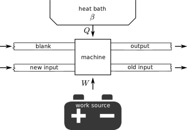
Figure 2: Sketch of the general setup, which allows us to analyze any abstract computational process in terms of thermodynamic quantities. The upper tape corresponds to the output tape, which is initially blank, and the lower tape corresponds to the input tape. Note that we will always assume that blank tapes are for free, i.e., the machine can have as many blank space on which it can write as it requires. Furthermore, the machine itself has access to two additional internal tapes (not sketched), see Sec. III.2.

Examining the thermodynamics of computation can be done in many different ways. Here, as stressed in the introduction, we want to capture three main features: first, we want to look at a general computational problem and not one specific task; second, we are interested in a logically reversible computer; and third, we want to model the computation stochastically, i.e., as a Brownian computer. The general thermodynamic picture is hence as sketched in Fig. 2. Some machine (with a very complex interior in general, see below) is coupled to a thermal reservoir at inverse temperature $\beta$ and a work reservoir. The work reservoir can be used to drive the computation in a certain direction whereas the thermal reservoir is equipped with a well-defined notion of heat and entropy. The task of our machine is to compute. It therefore receives input signals and transforms them to output signals corresponding to the result of the computation. Logical reversibility demands that we use two separate tapes for the inputs and outputs (henceforth called the input and output tapes, respectively). In fact, if we do not keep the initial inputs but simply overwrite them with the output (as the TM from Sec. II would do), our machine will be in general irreversible .

More specifically, a logically reversible computer is in principle able to unambiguously retrace its computational path (i.e., the sequence of logical states visited so far) back to the initial state. In fact, most TMs as introduced in Sec. II are logically irreversible, for instance, already due to the fact that the machines usually do not remember from which direction they were coming from. But even if it would remember this (for instance by writing the direction $d$ on an additional tape), the machine might still be logically irreversible. Consider for example that there exists a pair of states and symbols $(q_{1},s_{1})$ and $(q_{2},s_{2})$ such that $q^{\prime}=F(q_{1},s_{1})=F(q_{2},s_{2})$, $s^{\prime}=G(q_{1},s_{1})=G(q_{2},s_{2})$ and $d^{\prime}=H(q_{1},s_{1})=H(q_{2},s_{2})$. Then, given the state $(q^{\prime},s^{\prime})$ [or even $(q^{\prime},s^{\prime},d^{\prime})$], the machine has two possible predecessor states and it cannot know from which it was coming. Hence, it is logically irreversible. This situation is sometimes called the merging of two computational paths, see Fig. 3.

However, even a logically reversible computer still proceeds deterministically step by step along its computational path. This deterministic behaviour unambigously defines a computational direction, see Fig. 3 again (we remark that the computational direction does not necessarily coincide with the “physical” direction of the movement of the tape, which can – as we have seen – be shifted either way). In contrast, we also want to look at a stochastic machine, which makes random transitions in both directions, i.e., it is also allowed to jump back to a previous computational state. In order to assure that we can control the direction of computation on average, we demand that we can change the potential energy externally, for instance, by using a work source or by adjusting chemical potentials appropriately.

In the next section we will present the main ideas of how to obtain a logically reversible TM from an irreversible TM as discussed in Sec. II sparing the mathematical details to the appendix. Then, given that we have a logically reversible TM, we will show how to associate a ME to it in Sec. III.3.

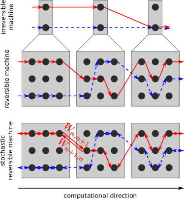
Figure 3: A computational path is defined by the way the machine proceeds from state to state through a high-dimensional state space (each state of the machine including the tapes is symbolized by a black circle). Here, we sketched two different paths (solid red and dashed blue lines). For standard machines (which compute only from left to right) each path is uniquely determined by the input signal string and the initial machine state. For a logically irreversible machine, however, it might happen that two different paths merge at some point (as shown on top) making it impossible to find the inverse of a state in general (that is to say there is a unique way to go from left to right in the diagram but not from right to left). In contrast, this cannot happen for logically reversible machines (as shown in the middle), but this feature comes at the cost of introducing additional states and tapes making the state space even larger. Finally, whereas the standard logically reversible TM still proceeds deterministically from left to right, a stochastic TM jumps randomly according to some rates [e.g., $W_{n+1,n}$ and $W_{n,n+1}$ as used in Eqs. (6) and (8)] and hence, it can move both ways (bottom).

III.2 Logically reversible Turing machine

The procedure to make a computation of a TM logically reversible was explained in detail in a famous publication by Bennett BennettIBM1973 . He explicitly showed – given an arbitrary TM $T$ as described by Eq. (1) – how to construct a machine $R$ which is computationally equivalent to $T$ but always logically reversible. To accomplish this, Bennett introduced a finite number of new machine states and two additional tapes, which record the previous computational steps taken. Furthermore, the computation is broken up into three stages (each stage in general consists of many single computational steps) and in total, the logically reversible TM needs approximately four times as many steps as the irreversible one BennettIBM1973 . Before we proceed, we remark that the construction given by Bennett is, of course, not unique (as he discusses as well) but seems to be very convenient. It is also noteworthy that TMs acting on $n$ tapes are not more powerful (in terms of what they can compute) than a TM described by Eq. (1) because one can be mapped onto the other MinskyBook .

In addition to the treatment of Bennett, who considered only a single computation $T:\textbf{s}_{\text{in}}\rightarrow\textbf{s}_{\text{out}}$, we want to construct a machine which continuously processes a stream of incoming input strings of the form $(\dots b,\textbf{s}^{\prime}_{\text{in}},b,\dots,b,\textbf{s}_{\text{in}},b,\dots)$. Thus, we imagine an infinite input tape with different input strings $\textbf{s}_{\text{in}},\textbf{s}^{\prime}_{\text{in}},\dots$ separated by blank symbols to mark the beginning and the end of each single input string. The output tape then contains the results of the different computations, i.e., it looks like $(\dots,b,\textbf{s}^{\prime}_{\text{out}}=T(\textbf{s}^{\prime}_{\text{in}}),b,\dots,b,\textbf{s}_{\text{out}}=T(\textbf{s}_{\text{in}}),b\dots)$. In this picture our machine resembles the devices from Refs. MandalJarzynskiPNAS2012 ; BaratoSeifertEPL2013 ; MandalQuanJarzynskiPRL2013 ; DeffnerJarzynskiPRX2013 ; BaratoSeifertPRE2014 ; StrasbergEtAlPRE2014 in which also an external tape is manipulated but mainly to extract work and not for computational purposes though.

stage	input tape	working tape	history tape	output tape	short form, see Eq. (4)
	input				$T_{5}T_{4}T_{3}T_{2}T_{1}(\textbf{s}_{\text{in}},\textbf{b},\textbf{b},\textbf{b})$
1) copy input onto working tape
	input	input			$T_{5}T_{4}T_{3}T_{2}(\textbf{s}_{\text{in}},\textbf{s}_{\text{in}},\textbf{b},\textbf{b})$
2) compute
	input	output	history		$T_{5}T_{4}T_{3}(\textbf{s}_{\text{in}},\textbf{s}_{\text{out}},\textbf{h},\textbf{b})$
3) copy output to output tape
	input	output	history	output	$T_{5}T_{4}(\textbf{s}_{\text{in}},\textbf{s}_{\text{out}},\textbf{h},\textbf{s}_{\text{out}})$
4) retrace computation
	input	input		output	$T_{5}(\textbf{s}_{\text{in}},\textbf{s}_{\text{in}},\textbf{b},\textbf{s}_{\text{out}})$
5) erase working tape
	input$\star$			output	$(\textbf{s}_{\text{in}}\star,\textbf{b},\textbf{b},\textbf{s}_{\text{out}})$

Table 1: One computational cycle consists of five stages where each stage can consist of many steps. The first line shows the initial situation of the tapes. After the first stage, the tapes are shown as in the second line, which serves as the initial state for the second stage and so on. The underbar denotes the current position of the machine head on the respective tapes. Note that at each stage the machine works with two tapes only, whereas the other two remain unchanged. Furthermore, in the very last line we used a $\star$ to mark the input the computer has already processed, see appendix A for details.

Our logically reversible TM thus will have in total four tapes and one computational cycle proceeds in five stages. The four tapes are called the input, working, history and output tape. Whereas the input and output tape are supplied externally (see Fig. 2), the working and history tape belong to the machine itself. By this we especially want to emphasize that we require them to be blank at the end of the computation such that they are ready for usage again . More specifically, one computational cycle consists of the following five stages (also see Table 1):

1. Copy input onto working tape: A new input arrives at the machine on the input tape and the machine copies this input onto its working tape leaving it there in standard format at the end of the first stage.

2. Compute: In this stage the actual computation is performed which finally maps the input to the output. Furthermore, a history tape keeps track of the intermediate steps such that the computer would be able to retrace each step.

3. Copy output to output tape: If the computation halts, the output on the working tape is copied to the output tape and the working tape is reset to its position as at the end of stage 2.

4. Retrace computation: The computer retraces all its computation such that the output on the working tape becomes the input and the history is blank again. This stage is the inverse of stage 2.

5. Erase working tape: We erase the working tape with the help of the input tape such that the working tape is blank again. Note that this erasure step is logically reversible because we have an identical copy of the input on the input tape. Finally, we use an additional symbol ($\star$) to mark that we already performed a computation for the current input and the machine moves on to the next input on the input string.

Stage 2, 3 and 4 were already treated by Bennett in Ref. BennettIBM1973 . In addition, we require stages 1 and 5 because we want that our machine works continuously and not only once. The reader who is curious about the details of each step is refered to appendix A. Otherwise, instead of one big machine $T$ doing a computation in five stages, it might also help to imagine five small machines $T_{1},\dots,T_{5}$. Our big machine $T$ is then nothing else than a composition or concatenation of these small machines, i.e., $T=T_{5}\circ T_{4}\circ T_{3}\circ T_{2}\circ T_{1}\equiv T_{5}T_{4}T_{3}T_{2}T_{1}$ (similar to the composition of different functions). The action of $T$ on the state of the four tapes (in the order of the input, working, history and output tape, respectively) can be written as

$$\begin{split}\text{1) }&T_{5}T_{4}T_{3}T_{2}T_{1}(\textbf{s}_{\text{in}},\textbf{b},\textbf{b},\textbf{b})=T_{5}T_{4}T_{3}T_{2}(\textbf{s}_{\text{in}},\textbf{s}_{\text{in}},\textbf{b},\textbf{b}),\\ \text{2) }&T_{5}T_{4}T_{3}T_{2}(\textbf{s}_{\text{in}},\textbf{s}_{\text{in}},\textbf{b},\textbf{b})=T_{5}T_{4}T_{3}(\textbf{s}_{\text{in}},\textbf{s}_{\text{out}},\textbf{h},\textbf{b}),\\ \text{3) }&T_{5}T_{4}T_{3}(\textbf{s}_{\text{in}},\textbf{s}_{\text{out}},\textbf{h},\textbf{b})=T_{5}T_{4}(\textbf{s}_{\text{in}},\textbf{s}_{\text{out}},\textbf{h},\textbf{s}_{\text{out}}),\\ \text{4) }&T_{5}T_{4}(\textbf{s}_{\text{in}},\textbf{s}_{\text{out}},\textbf{h},\textbf{s}_{\text{out}})=T_{5}(\textbf{s}_{\text{in}},\textbf{s}_{\text{in}},\textbf{b},\textbf{s}_{\text{out}}),\\ \text{5) }&T_{5}(\textbf{s}_{\text{in}},\textbf{s}_{\text{out}},\textbf{b},\textbf{s}_{\text{out}})=(\textbf{s}_{\text{in}}\star,\textbf{b},\textbf{b},\textbf{s}_{\text{out}}).\end{split}$$ (4)

Eq. (4) can be regarded as a short form of Table 1. Here, b denotes a blank tape and h denotes the history tape at the end of stage 2. Clearly, if all the machines $T_{1},\dots,T_{5}$ are logically reversible, then also $T$ is.

III.3 Stochastic Turing machine

In this section we will show how to use a continuous-time Markov process to model any logically reversible TM, which we will simply call a stochastic TM. We start, however, by repeating what a ME is and what we need for a consistent thermodynamic interpretation.

A continuous-time Markov process describing the dynamics of a system $X$ corresponds to a set of states ${\cal{X}}$ and an associated probability $p_{x}$ to be in a state $x\in{\cal{X}}$, which changes according to a Markovian first order differential equation called the ME VanKampenBook :

$$\frac{d}{dt}p_{x}(t)=\sum_{x^{\prime}}W_{x,x^{\prime}}p_{x^{\prime}}(t).$$ (5)

Here, the rate matrix $W_{x,x^{\prime}}$ has real-valued entries and fulfills $\sum_{x}W_{x,x^{\prime}}=0$ for all $x^{\prime}\in{\cal{X}}$. This guarantees that probability is conserved throughout the evolution, i.e., $\frac{d}{dt}\sum_{x}p_{x}(t)=0$ for all $t$. If we want to equip the ME (5) with a thermodynamic interpretation SchnakenbergRMP1976 , we have to associate to each state $x$ an energy $E_{x}\in\mathbb{R}$ and the rate matrix has to additionally fulfill a property called local detailed balance, which states that $\ln[W_{x,x^{\prime}}/W_{x^{\prime},x}]=-\beta(E_{x}-E_{x^{\prime}})$ where $\beta$ is the inverse temperature of the environment to which the system $X$ has contact. Note that this automatically implies that, if $W_{x,x^{\prime}}\neq 0$, then also $W_{x^{\prime},x}\neq 0$, i.e., for each transition $x^{\prime}\rightarrow x$ the reversed one $x\rightarrow x^{\prime}$ must also exist. This framework can also be extended to more general situations involving, e.g., multiple environments at different temperatures SchnakenbergRMP1976 , but we do not need more than the things just mentioned.

Now, associating a ME to a logically reversible deterministic TM is in fact very easy. All we have to do is to change the (unidirectional) deterministic updating rules from appendix A into (bidirectional) probabilistic transition rules, i.e., we allow for transitions in the computational forward direction as well as transitions which just undo the last computational step (backward direction).

It is worth pointing out that the underlying state space ${\cal{X}}$ of the ME is in general infinite, but this is not necessarily related to the size of the input tape. Remember that – due to the halting problem – a computation might go on forever even if it only received a finite input. In fact, even if the computation halts, there is no general way to give a reasonable estimate of the size of ${\cal{X}}$ in advance MinskyBook . However, on the other hand, the structure of the ME is very simple and this is related to the fact that we build the machine in a logically reversible way. In fact, each state $x\in{\cal{X}}$ has only two adjacent states, namely its logical predecessor and its logical successor state. Hence, our ME describes a simple one-step or birth-and-death process VanKampenBook or equivalently, according to Schnakenberg SchnakenbergRMP1976 , we could say that the topology of the underlying network is trivial. In fact, if there were any branchings or loops in the underlying network, the computation would not be logically reversible anymore because then a state could have multiple predecessors or successors. Hence, quite generally we can put the final ME into the form

$$\begin{split}\frac{d}{dt}p_{n}(t)=&-(W_{n+1,n}+W_{n-1,n})p_{n}(t)\\ &+W_{n,n+1}p_{n+1}(t)+W_{n,n-1}p_{n-1}(t).\end{split}$$ (6)

Here, of course, $n\in\mathbb{Z}$ is a multi-index denoting the entire machine and tape configuration.

Let us discuss the general structure of the ME a little further. First of all, it is important to note that only the current squares of the tapes can change stochastically whereas the rest of the tapes, which is not coupled to the machine, remains fixed. In fact, although there is an infinite number of possible different states, not all states $x\in{\cal{X}}$ are coupled with each other. Which states are coupled to each other is determined by the rules from appendix A and by the input strings $\textbf{s}_{\text{in}}$ because they single out a unique computational path through the “labyrinth” of states in ${\cal{X}}$.

In addition, the number of transition rules is always finite and fixed as expressed in appendix A. This is true independently of the number of computations or the lengths of the input strings. Although there seem to be quite a lot of rules, note that they suffice to build a universal logically reversible computer. Of course, things become much easier if we relax some of the requirements. Hence, in a more pictorial language we could say that the hardware (i.e., the set of transitions rules with the associated rates) of our machine remains fixed, but the software (i.e., the inputs determining the computational path) can change.

Thus, if we focus only on the computation for one input string, i.e., on the stages 2 to 4, the full rate matrix $W$ in Eq. (5) decomposes into blocks for each input string s, i.e., it has the form

$$W=\left(\begin{array}[]{cccc}\boxed{W(\textbf{s}_{1})}&&&\\ &\boxed{W(\textbf{s}_{2})}&&\\ &&\boxed{W(\textbf{s}_{3})}&\\ &&&\ddots\\ \end{array}\right)$$ (7)

and no transition between different blocks is allowed. Here, we labeled the different input strings $\textbf{s}_{1},\textbf{s}_{2},\textbf{s}_{3},\dots$ in some canonical way and note that each block can be infinitely large if the computation does not halt. For each $\textbf{s}_{i}$ the ME describes a simple one-step process and by rearranging the states appropriately we can write each block as a tridiagonal matrix

$$W(\textbf{s}_{i})=\left(\begin{array}[]{ccccc}\ddots&&&&\\ &-W_{n,n-1}-W_{n-2,n-1}&W_{n-1,n}&0&\\ &W_{n,n-1}&-W_{n+1,n}-W_{n-1,n}&W_{n,n+1}&\\ &0&W_{n+1,n}&-W_{n+2,n+1}-W_{n,n+1}&\\ &&&&\ddots\\ \end{array}\right)$$ (8)

where $W_{n+1,n}$ ($W_{n-1,n}$) denotes the forward (backward) rate at step $n$ in the ME (6). Hence, to conclude, although the state space ${\cal{X}}$ is extremely large, the rate matrix is also extremely sparse, i.e., it contains only a small number of non-zero elements (in relation to the total number of elements).

Finally, we would need to associate a consistent energy landscape to our system and the rate of forward and backward transitions would then need to obey local detailed balance, which fixes the temperature of the environment. We will discuss this issue in the next section.

IV Thermodynamics of Brownian computation

IV.1 Energy landscapes

So far we have shown that a stochastic, logically reversible TM can be modeled by a simple one-step process as given by the ME (6). To interpret it thermodynamically we still need to associate a consistent energy landscape to it, which we could control externally via a work source or, alternatively, a bias in chemical potentials as it would be the case for biochemical processes.

For the sake of simplicity, we will choose below a linear energy landscape along the computational path, i.e., the difference in energy between a logical state and its successor state is taken to be the constant $\epsilon$ (i.e., for $\epsilon>0$ the computation proceeds on average in the forward direction along a chain of states with decreasing energies). This choice is in agreement with the one usually appearing in the literature BennettIBM1973 ; Bennett1982 ; Feynman1985 ; NortonFoundPhys2013 . Before we proceed, however, we discuss and justify this choice in more detail.

First of all, in Sec. IV.2 we will actually discuss the thermodynamics of our model on a coarse-grained level of description. That is to say we will be interested in the regime where the computer was running already for quite a long time such that the variance ${\langle{n^{2}}\rangle}-{\langle{n}\rangle}^{2}$ of the number of computational steps is large compared to unity where we defined ${\langle{n^{\ell}}\rangle}\equiv\sum_{n}n^{\ell}p_{n}(t)$. In this picture, $\epsilon$ might denote just an average slope in the energy landscape, i.e., we explicitly allow for spatial irregularities in the energy landscape as long as they are not too large. More specifially, if $E_{n}$ denotes the energy of state $n$ according to the ME (6), we demand that

$$\epsilon\overset{!}{=}\frac{1}{2N}\sum_{n=-N}^{N-1}(E_{n}-E_{n+1})$$ (9)

holds for all $n$ and for $N$ of the order of the variance ${\langle{n^{2}}\rangle}-{\langle{n}\rangle}^{2}$ such that the energy landscape looks linear at the coarse-grained level.

Second, it is worth pointing out that in fact – except for the spatially allowed irregularities – no other energy landscape seems to be feasible for a general purpose computer. The reason for this is twofold: first, we are interested in a steady state regime, i.e., the average dissipation per step should be independent of the number of computational steps performed so far. This demand rules out quadratic or exponential energy landscape. Second, we are also still faced with the halting problem. This implies that we cannot know in advance the number of computational steps we need for one computational cycle. Thus, associating any particularly shaped energy landscapes like a sine or a hill (as in NortonIntJModPhys2014 ) is unfeasible because we do not know, for instance, how to choose a senseful period for the sine.

Hence, we conclude: the only feasible energy landscape with which we can ensure to control the speed and direction of computation independently of the number of computational steps (which we cannot know in advance) and which is translationally invariant on the state space $n\in\mathbb{Z}$ of the ME (6) is an on average linear landscape.

IV.2 Effective Fokker-Planck equation

Having agreed on the (on average) linear energy landscape we will choose the transition rates in Eq. (6) as follows:

$$W_{n,n+1}=\Gamma e^{-\beta\epsilon/2},~{}~{}~{}W_{n+1,n}=\Gamma e^{\beta\epsilon/2}.$$ (10)

Here, $\Gamma$ is some rate setting the overall time-scale of our problem and we see that the rates fulfill local detailed balance, i.e., $\ln[W_{n,n+1}/W_{n+1,n}]=-\beta(E_{n}-E_{n+1})=-\beta\epsilon$ where $\beta\epsilon>0$ favors a computation in the forward direction.

In the limit where the mean $\langle n\rangle$ and variance ${\langle{n^{2}}\rangle}-{\langle{n}\rangle}^{2}$ are large compared to one, we can approximate derivatives by

$$\begin{split}\frac{\partial}{\partial n}p_{n}(t)&\approx\frac{p_{n+1}(t)-p_{n-1}(t)}{2},\\ \frac{\partial^{2}}{\partial n^{2}}p_{n}(t)&\approx p_{n+1}(t)-2p_{n}(t)+p_{n-1}(t).\end{split}$$ (11)

Then, the Fokker-Planck equation (FPE) corresponding to the ME (6) reads

$$\frac{1}{\Gamma}\frac{\partial}{\partial t}p_{n}(t)=\frac{\partial}{\partial n}\left[-2\sinh\frac{\beta\epsilon}{2}+\cosh\frac{\beta\epsilon}{2}\frac{\partial}{\partial n}\right]p_{n}(t).$$ (12)

This FPE describes the movement of an overdamped Brownian particle in a constant force field and with a constant diffusion coefficient with $n\in\mathbb{R}$ denoting the position of the particle. It even admits an explicit solution: assuming that the machine has started initially at some fixed state $n=0$, i.e., $p_{n}(t=0)=\delta(n)$, we obtain

$$\begin{split}p_{n}(t)=&~{}\frac{1}{\sqrt{4\pi\Gamma\cosh(\beta\epsilon/2)t}}\\ &\times\exp\left\{-\frac{[n-2\Gamma\sinh(\beta\epsilon/2)t]^{2}}{4\Gamma\cosh(\beta\epsilon/2)t}\right\}.\end{split}$$ (13)

IV.3 Thermodynamic discussion

Discussing the thermodynamic behaviour of Eq. (12) can be done using standard methods, see e.g. Ref. SekimotoBook . We first of all compute the mean number of computational steps, which is

$${\langle{n}\rangle}(t)=2\Gamma t\sinh\frac{\beta\epsilon}{2}$$ (14)

and hence, the speed of computation becomes

$$v\equiv\frac{d}{dt}{\langle{n}\rangle}(t)=2\Gamma\sinh\frac{\beta\epsilon}{2},$$ (15)

which – as expected – can be controlled by $\epsilon$. Especially, we see that we have $v>0$ for $\epsilon>0$ and vice versa.

The variance of the distribution is

$${\langle{n^{2}}\rangle}(t)-{\langle{n}\rangle}^{2}(t)=2\Gamma t\cosh\frac{\beta\epsilon}{2}$$ (16)

and grows linearly with time. Based on this we might ask the question when does the computation become approximately deterministic, i.e., when does the mean dominate the standard deviation? Calculating their ratio yields

$$\frac{{\langle{n}\rangle}(t)}{\sqrt{{\langle{n^{2}}\rangle}(t)-{\langle{n}\rangle}^{2}(t)}}=\sqrt{2\Gamma t\tanh\frac{\beta\epsilon}{2}\sinh\frac{\beta\epsilon}{2}}.$$ (17)

If we want this quantity to be much larger than one, we obtain a condition for the minimum amount of time we have to wait until our machine computes almost in a deterministic fashion:

$$t\gg\left(2\Gamma\tanh\frac{\beta\epsilon}{2}\sinh\frac{\beta\epsilon}{2}\right)^{-1}\approx\frac{2}{\Gamma\beta^{2}\epsilon^{2}}.$$ (18)

Here, we performed an expansion in $\beta\epsilon\ll 1$ at the end. Thus, the closer we get to the reversible limit, i.e., the smaller $\beta\epsilon$ (see below), the longer we have to wait until the computer starts to work reliably.

Furthermore, we can explicitly calculate the Shannon entropy of our distribution, which is

$$H(t)\equiv-\int dnp_{n}(t)\ln p_{n}(t)=\frac{1}{2}\ln\left(4\pi e\Gamma t\cosh\frac{\beta\epsilon}{2}\right).$$ (19)

Using Eq. (14) we can also write the Shannon entropy as

$$H(t)=\frac{1}{2}\ln\left[2\pi e\coth\left(\frac{\beta\epsilon}{2}\right){\langle{n}\rangle}(t)\right],$$ (20)

i.e., the Shannon entropy scales with the average number ${\langle{n}\rangle}$ of computational steps as $S(t)\sim\ln{\langle{n}\rangle}$.

The rate at which entropy is produced is given by the change in Shannon entropy plus $\beta$ times the heat flow dissipated into the environment SekimotoBook . Since the latter is simply $\epsilon v$, we can write for the entropy production rate

$$\begin{split}\dot{S}_{\textbf{i}}(t)&=\frac{d}{dt}H(t)+\beta\epsilon v\\ &=\frac{1}{2t}+2\Gamma\beta\epsilon\sinh\frac{\beta\epsilon}{2}\geq 0.\end{split}$$ (21)

We now note that for $\epsilon\rightarrow 0$ the last term vanishes quadratically, i.e., the heat dissipated can be made arbitrarily small in this limit. The first term, however, is independent of $\epsilon$ but vanishes for $t\rightarrow\infty$. Hence, we have

$$\lim_{t\rightarrow\infty}\lim_{\epsilon\rightarrow 0}\dot{S}_{\textbf{i}}(t)=0.$$ (22)

Thus, a Brownian computer can work thermodynamically reversibly (i.e., with zero entropy production rate) in the steady state regime if the bias $\epsilon$ is small enough. This would confirm the conclusions from Ref. BennettIBM1973 ; Bennett1982 ; Feynman1985 .

However, we can also confirm Norton’s perspective on the matter NortonFoundPhys2013 ; NortonIntJModPhys2014 . Starting initially at $t=0$ we see that the total amount of entropy produced up to time $t$ is

$$\Delta_{\textbf{i}}S(t)=\int_{0}^{t}dt^{\prime}\dot{S}_{\textbf{i}}(t^{\prime})=H(t)+\beta\epsilon{\langle{n}\rangle}(t)\geq 0.$$ (23)

Thus, even for $\epsilon=0$ the Shannon entropy still grows logarithmically with the number of computational steps because the probability distribution of the machine spreads over the available phase space similarly to the free expansion of a one-molecule gas, which is a thermodynamically irreversible process. If we think in terms of thermodynamic cycles instead of a thermodynamic machine, which works in the stationary regime, we would have to dissipate an amount of entropy proportional to $\ln{\langle{n}\rangle}$ to reset the Brownian computer to its initial zero entropy state. However, again, compared to the number of computational steps ${\langle{n}\rangle}$ taken, the ratio $\ln({\langle{n}\rangle})/{\langle{n}\rangle}$ becomes arbitrarily small for a large number of steps, i.e., for a long computation.

Finally, we remark that a full treatment in terms of the ME (6) instead of the FPE (12) would provide very similar results. In fact, the first two cumulants (mean and variance) can be shown to coincide.

V Summary and outlook

Let us summarize our main findings and discuss possible interesting open questions based on our findings.

We have started with an arbitrary TM as a model for a general purpose computer, which is, however, in general logically irreversible and free from any thermodynamic interpretation. We then discussed how a computation can be regarded as a thermodynamic process and we decided to investigate the thermodynamics of a logically reversible stochastic computer, which simulates the TM considered at the beginning. We explained in detail how to obtain a logically reversible computer out of an irreversible one and then used bidirectional probabilistic transition rules instead of unidirectional deterministic rules to model the stochastic or random motion of our computer.

Although the problem seems to be very complex, we have seen that the resulting ME has the very simple structure of a one-step process, which describes how the computer follows a well-defined path in a large state space and eventually maps the input signals to output signals (the results of the computation). We have argued that the only feasible energy landscape for such a computer is an approximately linear one, which not only simplified the thermodynamic discussion, but also allowed us to solve a corresponding FPE describing the drift and diffusion of the computer exactly.

We have then seen that our stochastic computer can work thermodynamically reversibly, i.e., in a dissipation-free fashion, in a steady state regime and in this respect Feynman was indeed right with his initially quoted statement. However, just because the entropy production rate can become arbitrary small, this does not imply that the overall integrated entropy production is zero. Especially, if we think in terms of a computational cycle, in which we want to reset the computer to its initial state at the end, there is an unavoidable cost due to the increasing Shannon entropy of the probability distribution during the computation. In fact, this additional cost is not independent of the number of computational steps but scales logarithmically with it and it seems that this effect has been only recognized by Norton so far NortonFoundPhys2013 . Here, we have verified this result in a conceptually clean and general framework.

Furthermore, it is worth emphasizing that our computer works error-free at a finite entropy production. In fact, by construction our model does only allow for temporary errors in the computation (due to the fact that our stochastic machine can randomly hop back to its previous state), but in the long run each temporary error is corrected by the next step in the computational forward direction and there are no other sources of errors allowed. Including errors (for instance, random bit flips or – to avoid the halting problem and an infinitely long computation – one could decide to terminate the computation after a fixed number $N_{\text{max}}$ of steps) in our scheme and investigating the thermodynamic cost to correct them might be an interesting project for the future.

Another interesting question is whether we can sensefully assign a notion of efficiency to our computer. From a purely physical point of view the machine we have considered is actually senseless because it describes only a simple (and never-ending) relaxation process. However, the machine is indeed “working”, i.e., doing something “useful” for us, because it tells us the answer to many questions. But how can we quantify the usefulness of our machine? Having a rigorous notion of a thermodynamic efficiency for a computer would allow us to study question of, e.g., efficiency at maximum power, which is an important question for the design of realistic machines, see, e.g., CurzonAhlbornAJP1975 ; VandenBroeckPRL2005 ; SchmiedlSeifertEPL2008 ; EspositoLindenbergVandenBroeckPRL2009 ; EspositoLindenbergVandenBroeckEPL2009 . In this context, one can also ask the question whether a logically reversible computer is really desirable or whether a logically irreversible computer might indeed be able to work at a fundamentally better efficiency. At the end, it seems that biochemical processes in our body work very efficiently, but not necessarily in a logically reversible way.

Finally, let us say a few words about the relation between the present work and the devices investigated in Refs. MandalJarzynskiPNAS2012 ; BaratoSeifertEPL2013 ; MandalQuanJarzynskiPRL2013 ; DeffnerJarzynskiPRX2013 ; BaratoSeifertPRE2014 ; StrasbergEtAlPRE2014 (also see Feynman for a simple example of such a device who called them information-driven engines Feynman1985 ). Indeed, as in our case, these information-driven engines are coupled to an external tape or “information reservoir”. This additional reservoir can then be used to extract work from a single heat bath while simultaneously writing information on the tape (i.e., increasing its Shannon entropy). This picture, however, does not carry over to our situation. In fact, the Shannon entropies of the incoming and outgoing tapes are equal because the input tape gets mapped to itself and the output tape is uniquely determined by the input. For a logically irreversible computer this does not need to be true as it can be already seen from the devices in Refs. MandalJarzynskiPNAS2012 ; BaratoSeifertEPL2013 ; MandalQuanJarzynskiPRL2013 ; DeffnerJarzynskiPRX2013 ; BaratoSeifertPRE2014 ; StrasbergEtAlPRE2014 where it was also shown that they can be used as an information eraser.

Appendix A Logical reversible Turing machine

We here provide the detailed rules for the machine behaviour at each stage of the computation. These rules are, of course, not unique. However, because we are not primarily interested in the speed or efficiency of our machine, but only in what it can do, possibly different implementations are unimportant for the present context. Furthermore, note that at each stage the machine is only manipulating two tapes whereas the other two tapes remain fixed (see Table 1). We will therefore use the notation $[q^{(i)},s_{m},t_{n}]$ where $q^{(i)}$ denotes the internal machine state at stage $i$, $s_{m}$ the symbol $s$ printed on square $m$ of the first tape of interest and $t_{n}$ the symbol $t$ printed on square $n$ of the second tape of interest. What are the tapes of interest will become clear in the treatment of each stage. Note that the notation is different from the one used by Bennett BennettIBM1973 .

A.1 Stage 1) copy input onto working tape

We want to copy the input on the input tape (first tape of interest) to the working tape (second tape of interest). The input is given in the form $\textbf{s}_{\text{in}}=(s_{1},\dots,s_{M})$ and we assume that the machine scans initially the symbol at the far right (i.e., $s_{M}$) (see also Table 1). Furthermore, the working tape is by construction initially completely blank (that this is so can only be seen after the completion of all five stages, of course). The copy stage then proceeds as follows:

$$\begin{split}[q_{0}^{(1)},(s_{M})_{m},b_{n}]\rightarrow&~{}[q_{1}^{(1)},(s_{M})_{m},(s_{M})_{n}]\\ \rightarrow&~{}[q_{0}^{(1)},(s_{M-1})_{m-1},b_{n-1}]\\ \rightarrow&~{}[q_{1}^{(1)},(s_{M-1})_{m-1},(s_{M-1})_{n-1}]\\ &~{}\vdots\\ \rightarrow&~{}[q_{1}^{(1)},(s_{1})_{m-(M-1)},(s_{1})_{n-(M-1)}]\\ \rightarrow&~{}[q_{0}^{(1)},b_{m-M},b_{n-M}]\\ \rightarrow&~{}[\text{R}^{(2)},b_{m-M},b_{n-M}].\end{split}$$ (24)

Hence, we see that during the copy operation the machine changes between the two states $q_{0}^{(1)}$ and $q_{1}^{(1)}$ where the first is responsible for copying the symbol on the input tape to the working tape and the second is responsible for a shift of both tapes. This procedure goes on until it hits the first blank symbol to the left of the input string. The machine then changes to the “ready” state R⁽²⁾, which is the special initial state for the second stage. Note that – due to the fact that the copying procedure is unidirectional, i.e., the machine moves the tape always in the same direction – each map has a clear logical inverse. Furthermore, the positions $m$ and $n$ of the squares are in general arbitrary and can be chosen initially at will.

A.2 Stage 2) compute

This is the central stage of our computational cycle. If we would not bother about logical reversibility, this would be the only stage to execute. We thus have to explicitly think about how to make the map (1) logically reversible. The idea is the following BennettIBM1973 : first, because each standard (i.e., irreversible) TM is defined by its $N_{{\cal{Q}}}(N_{{\cal{S}}}+1)$ many quintuples, we introduce a set $\tilde{Q}$ with $\#\tilde{Q}=N_{{\cal{Q}}}(N_{{\cal{S}}}+1)$ of additional machine states $\tilde{q}\in\tilde{Q}$. Then, to each map $(q,s)\rightarrow(q^{\prime},s^{\prime},d^{\prime})$ we can associate a special state $\tilde{q}_{qs}$, which uniquely labels each quintuple. Second, we will make use of an additional tape called the history tape, which remembers the past $\tilde{q}_{qs}$ such that the machine is able to uniquely retrace its computational path.

Stage 2 is thus a bit more complicated. The corresponding maps are

$$\begin{split}[\text{R}^{(2)},b_{n-M},b_{m}]&~{}~{}~{}\rightarrow[\tilde{q}^{(2)}_{R^{(2)}b},b_{n-M},b_{m+1}]\\ &~{}~{}~{}\rightarrow[q_{1},(s_{1})_{n-M+1},(\tilde{q}_{\text{R}^{(2)}b})_{m+1}]\\ &~{}~{}~{}~{}~{}~{}~{}~{}\vdots\\ \text{step }\ell&\left\{\begin{array}[]{ll}\rightarrow&[q_{\ell}^{(2)},(s_{\ell})_{n^{\prime}},(\tilde{q}_{q_{\ell-1}^{(2)}s_{\ell-1}})_{m+\ell}]\\ \rightarrow&[\tilde{q}^{(2)}_{q_{\ell}^{(2)}s_{\ell}},(s^{\prime}_{\ell})_{n^{\prime}},b_{m+\ell+1}]\\ \rightarrow&[q^{\prime(2)}_{\ell},(s_{\ell+1})_{n^{\prime}+d^{\prime}},(\tilde{q}_{q_{\ell}^{(2)}s_{\ell}})_{m+\ell+1}]\\ \end{array}\right.\\ &~{}~{}~{}~{}~{}~{}~{}~{}\vdots\\ \text{step }\nu&~{}~{}~{}\rightarrow[\tilde{q}^{(2)}_{q_{\nu}^{(2)}s_{\nu}},(s^{\prime}_{\nu})_{n^{\prime\prime}-1},b_{m+\nu+1}]\\ &~{}~{}~{}\rightarrow[\text{H}^{(2)},b_{n^{\prime\prime}},(\tilde{q}_{q_{\nu}^{(2)}s_{\nu}})_{m+\nu+1}].\end{split}$$ (25)

The most important step to understand is the one in the middle, which corresponds to the $\ell$’th computational step of the ordinary irreversible TM defined by (1). Initially, the machine is in state $q_{\ell}^{(2)}$ and scans the symbol $s_{\ell}$ on the square $n^{\prime}$ of the working tape. The history tape contains the state $\tilde{q}^{(2)}_{q_{\ell-1}^{(2)}s_{\ell-1}}$, which uniquely labels the previous computational step. Then, the machine changes its state to $\tilde{q}^{(2)}_{q_{\ell}^{(2)}s_{\ell}}$, writes the symbol $s^{\prime}_{\ell}$ on the square according to the function $s^{\prime}_{\ell}=G(q^{(2)}_{\ell},s_{\ell})$ and shifts the history tape one square to the left, which contains a blank symbol. Finally, we write $\tilde{q}_{q_{\ell}^{(2)}s_{\ell}}$ to the history tape and change the machine state to $q^{\prime(2)}_{\ell}=F(q^{(2)}_{\ell},s_{\ell})$. Furthermore, we shift the working tape one square according to $d^{\prime}=H(q^{(2)}_{\ell},s_{\ell})$ such that the machine now scans the new symbol $s_{\ell+1}$. Then, the whole procedure can start again where – in order that we are able to apply map (1) – we identify $q^{\prime(2)}_{\ell}\equiv q^{(2)}_{\ell+1}$ because the final state of the machine at the end of step $\ell$ is the initial state for step $\ell+1$.

The first and last two lines of Eq. (25) then simply describe the initial and final steps of the computation. Initially, the machines starts in R⁽²⁾ and then shifts the working tape to the left such that it reads the first symbol $s_{1}$ and starts in the state $q_{1}^{(2)}$. Finally, if the machine halts, it reaches the state H and stops at the first blank to the right of the output of the computation.

A.3 Stage 3) copy output to output tape

We now want to copy the output $\textbf{s}_{\text{out}}=(s_{1},\dots,s_{M^{\prime}})$ of the computation from stage 2 from the working tape (first tape of interest) to the output tape (second tape of interest). This goes as follows

$$\begin{split}[\text{H}^{(2)},b_{n^{\prime\prime}},b_{m}]\rightarrow&~{}[q_{0}^{(3)},b_{n^{\prime\prime}},b_{m}]\\ \rightarrow&~{}[q_{1}^{(3)},(s_{M^{\prime}})_{n^{\prime\prime}-1},b_{m-1}]\\ \rightarrow&~{}[q_{0}^{(3)},(s_{M^{\prime}})_{n^{\prime\prime}-1},(s_{M^{\prime}})_{m-1}]\\ &~{}\vdots\\ \rightarrow&~{}[q_{0}^{(3)},(s_{1})_{n^{\prime\prime}-M^{\prime}},(s_{1})_{m-M^{\prime}}]\\ \rightarrow&~{}[q_{1}^{(3)},b_{n^{\prime\prime}-M^{\prime}-1},b_{m-M^{\prime}-1}]\end{split}$$ (26)

and is very similar to (25). Finally, however, to prepare the machine for the next stage, we want that it scans the output on the working tape at the very right again (at the moment it scans the blank on the working tape to the left of the output). To accomplish this we use two more machine states:

$$\begin{split}&[q_{1}^{(3)},b_{n^{\prime\prime}-M^{\prime}-1},b_{m-M^{\prime}-1}]\\ &\rightarrow[q_{2}^{(3)},b_{n^{\prime\prime}-M^{\prime}-1},b_{m-M^{\prime}-1}]\\ &\rightarrow[q_{3}^{(3)},(s_{1})_{n^{\prime\prime}-M^{\prime}},b_{m-M^{\prime}-2}]\\ &\rightarrow[q_{3}^{(3)},(s_{2})_{n^{\prime\prime}-M^{\prime}+1},b_{m-M^{\prime}-3}]\\ &~{}~{}~{}~{}~{}\vdots\\ &\rightarrow[q_{3}^{(3)},(s_{M^{\prime}})_{n^{\prime\prime}-1},b_{m-2M^{\prime}}]\\ &\rightarrow[q_{3}^{(3)},b_{n^{\prime\prime}},b_{m-2M^{\prime}-1}].\end{split}$$ (27)

Here, $q_{2}^{(3)}$ is an intermediate state and its sole purpose is to indicate that the copying procedure is over and the machine starts now only to shift the working tape without changing it. The state $q_{3}^{(3)}$ then actually accomplishes this task by shifting the working tape one step to the left while simultaneously shifting the output tape one step to the right until it reaches the first blank symbol to the right of the output on the working tape, which will indicate the start of stage 4.

A.4 Stage 4) retrace computation

In this stage we will basically apply the inverse of stage 2 such that at the end the working tape contains the input again and the history tape is returned to its initial blank state. This goes as follows:

$$\begin{split}&[q_{3}^{(3)},b_{n^{\prime\prime}},(\tilde{q}_{q_{\nu}^{(2)}s_{\nu}})_{m+\nu}]\\ &\rightarrow[\text{H}^{(4)},b_{n^{\prime\prime}},(\tilde{q}_{q_{\nu}^{(2)}s_{\nu}})_{m+\nu}]\\ &\rightarrow[\tilde{q}^{(4)}_{q_{\nu}^{(2)}s_{\nu}},(s^{\prime}_{\nu})_{n^{\prime\prime}-1},b_{m+\nu}]\\ &\rightarrow[q_{\nu}^{(4)},(s^{\prime}_{\nu-1})_{n^{\prime\prime}-1},(\tilde{q}_{q_{\nu-1}^{(2)}s_{\nu-1}})_{m+\nu-1}]\\ &~{}~{}~{}~{}~{}\vdots\\ &\rightarrow[q^{\prime(4)}_{\ell},(s_{\ell+1})_{n^{\prime}+d^{\prime}},(\tilde{q}_{q_{\ell}^{(2)}s_{\ell}})_{m+\ell+1}]\\ &\rightarrow[\tilde{q}^{(4)}_{q_{\ell}^{(2)}s_{\ell}},(s^{\prime}_{\ell})_{n^{\prime}},b_{m+\ell+1}]\\ &\rightarrow[q_{\ell}^{(4)},(s_{\ell})_{n^{\prime}},(\tilde{q}_{q_{\ell-1}^{(2)}s_{\ell-1}})_{m+\ell}]\\ &~{}~{}~{}~{}~{}\vdots\\ &\rightarrow[q_{1}^{(4)},(s_{1})_{n-M+1},(\tilde{q}_{\text{R}^{(2)}b})_{m+1}]\\ &\rightarrow[\tilde{q}^{(4)}_{\text{R}^{(2)}b},b_{n-M},b_{m+1}]\\ &\rightarrow[\text{R}^{(4)},b_{n-M},b_{m}].\end{split}$$ (28)

Note that we are using the superscript $(4)$ on the internal machine states to explicitly distinguish them from the states of stage 2 indicating that we are truly in a different stage here.

A.5 Stage 5) erase working tape

The last step consists in erasing the content on the working tape such that it is blank again and ready for the next computation. Note that the “erasure” of the working tape does not actually erase any information because the working tape contains the same input $\textbf{s}_{\text{in}}=(s_{1},\dots,s_{M})$ as the input tape. As in stage 1 we choose the first tape of interest to be the input tape and the second tape of interest is the working tape. Then, we actually only have to apply the inverse of stage 1, i.e.,

$$\begin{split}[\text{R}^{(4)},b_{m-M},b_{n-M}]\rightarrow&~{}[q_{0}^{(5)},b_{m-M},b_{n-M}]\\ \rightarrow&~{}[q_{1}^{(5)},(s_{1})_{m-(M-1)},(s_{1})_{n-(M-1)}]\\ \rightarrow&~{}[q_{0}^{(5)},(s_{1})_{m-(M-1)},b_{n-(M-1)}]\\ &~{}\vdots\\ \rightarrow&~{}[q_{1}^{(5)},(s_{M})_{m},(s_{M})_{n}]\\ \rightarrow&~{}[q_{0}^{(5)},(s_{M})_{m},b_{n}]\\ \rightarrow&~{}[q_{1}^{(5)},b_{m+1},b_{n+1}].\end{split}$$ (29)

If we would postulate the final transition rule $[q_{1}^{(5)},b_{m+1},b_{n+1}]\rightarrow[q_{0}^{(1)},(s_{M})_{m},b_{n}]$ we would be exactly back at the initial state of stage 1 and the only change would be that we have printed the result of the computation on the output tape. However, if this were true, we would be doomed to repeat the same computation again, while in fact we want to compute with the next input $\textbf{s}^{\prime}_{\text{in}}$ on the input string. To achieve this we add the following rules:

$$\begin{split}[q_{1}^{(5)},b_{m+1},b_{n+1}]\rightarrow&~{}[q_{2}^{(5)},\star_{m+1},b_{n+1}]\\ \rightarrow&~{}[q_{2}^{(5)},(s_{M})_{m},b_{n+2}]\\ \rightarrow&~{}[q_{2}^{(5)},(s_{M-1})_{m-1},b_{n+3}]\\ &~{}\vdots\\ \rightarrow&~{}[q_{2}^{(5)},(s_{1})_{m-M},b_{n+M+1}]\\ \rightarrow&~{}[q_{2}^{(5)},b_{m-M-1},b_{n+M+2}]\\ \rightarrow&~{}[q_{3}^{(5)},b_{m-M-1},b_{n+M+2}]\\ &~{}\vdots\\ \rightarrow&~{}[q_{3}^{(5)},(s^{\prime}_{M^{\prime}})_{m^{\prime}},b_{\hat{n}}]\\ \rightarrow&~{}[q_{0}^{(1)},(s^{\prime}_{M^{\prime}})_{m^{\prime}},b_{\hat{n}}].\end{split}$$ (30)

Here, we first of all marked the input $\textbf{s}_{\text{in}}$ with a $\star$ to indicate that we have done already a computation for that input. We then used an additional state $q_{2}^{(5)}$, which simply traverses the input string $\textbf{s}_{\text{in}}$ until it hits a blank symbol. The machine then changes to the state $q_{3}^{(5)}$ and goes further to the left until it hits the next non-blank symbol on the input string. This symbol then indicates the beginning of the next input $\textbf{s}^{\prime}_{\text{in}}$ such that – starting from stage 1 again – we can readily execute the next computational cycle.

A.6 Summary

Suppose that the irreversible TM from Sec. II has $N_{{\cal{Q}}}$ many internal states, $N_{{\cal{S}}}+1$ many different symbols (including the blank) on the tape and hence, it has $N_{\tilde{Q}}\equiv N_{{\cal{Q}}}(N_{{\cal{S}}}+1)$ many quintuples. Furthermore, suppose it was given an input of length $M$ and produced an output of length $M^{\prime}$ after $\nu$ computational steps in total.

Then, our reversible machine has $2+(N_{{\cal{Q}}}+N_{\tilde{Q}})+4+(N_{{\cal{Q}}}+N_{\tilde{Q}})+4$ states from the first, second, …, fifth stage of the computation, i.e., in total $2(N_{{\cal{Q}}}+N_{\tilde{Q}})+10$ states. Furthermore, it needs $2M+2\nu+(2M^{\prime}+1)+2\nu+(2M+2+x)=4\nu+4M+2M^{\prime}+3+x$ many computational steps. Here, the $x$ denotes the number of unknown blank symbols separating the current input from the next input on the input tape (see stage 5). Note that we need $x\geq 2$ such that there is enough space for the symbol $\star$ and to guarantee that all input strings (including potentially the symbol $\star$) are separated by at least one blank symbol from eachother.

References

- (1) R. Landauer, Irreversibility and Heat Generation in the Computing Process, IBM J. Res. Dev. 5, 183 (1961).
- (2) C. H. Bennett, Logical Reversibility of Computation, IBM J. Res. Dev. 17, 525 (1973).
- (3) C. H. Bennett, The Thermodynamics of Computation – A Review, Int. J. Theor. Phys. 21, 905 (1982).
- (4) C. H. Bennett, Notes on the history of reversible computation, IBM J. Res. Dev. 32, 16 (1988).
- (5) R. W. Keyes and R. Landauer, Minimal Energy Dissipation in Logic, IBM J. Res. Dev. 14, 152 (1970).
- (6) K. Likharev, Classical and Quantum Limitations on Energy Consumption in Computation, Int. J. Theor. Phys. 21, 311 (1982).
- (7) C. H. Bennett and R. Landauer, The fundamental physical limits of computation, Scientific American 253, 48 (1985).
- (8) R. P. Feynman, Feynman Lectures on Computation (Addison-Wesley Publishing Company, 1996).
- (9) H. S. Leff and A. F. Rex (editors), Maxwell’s Demon 2: Entropy, Classical and Quantum Information, Computing (IOP Publishing, Bristol, 2003).
- (10) J. Earman and J. D. Norton, Exorcist XIV: The Wrath of Maxwell’s Demon. Part I. From Maxwell to Szilard, Stud. Hist. Phil. Mod. Phys. 29, 435 (1998).
- (11) J. Earman and J. D. Norton, Exorcist XIV: The Wrath of Maxwell’s Demon. Part II. From Szilard to Landauer and Beyond, Stud. Hist. Phil. Mod. Phys. 30, 1 (1999).
- (12) O. R. Shenker, Maxwell’s Demon and Baron Munchausen: Free Will as a Perpetuum Mobile, Stud. Hist. Phil. Mod. Phys. 30, 347 (1999).
- (13) J. Bub, Maxwell’s Demon and the Thermodynamics of Computation, Stud. Hist. Phil. Mod. Phys. 32, 569 (2001).
- (14) C. H. Bennett, Notes on Landauer’s principle, reversible computation, and Maxwell’s Demon, Stud. Hist. Phil. Mod. Phys. 34, 501 (2003).
- (15) O. J. E. Maroney, The (absence of a) relationship between thermodynamic and logical reversibility, Stud. Hist. Phil. Mod. Phys. 36, 355 (2005).
- (16) J. D. Norton, Eaters of the lotus: Landauer’s principle and the return of Maxwell’s demon, Stud. Hist. Phil. Mod. Phys. 36, 375 (2005).
- (17) J. Ladyman, S. Presnell, A. J. Short, and B. Groisman, The connection between logical and thermodynamic irreversibility, Stud. Hist. Phil. Mod. Phys. 38, 58 (2007).
- (18) M. Hemmo and O. R. Shenker, Maxwell’s demon, J. Philos. 107, 389 (2010).
- (19) J. D. Norton, Waiting for Landauer, Stud. Hist. Phil. Mod. Phys. 42, 184 (2011).
- (20) L. B. Kish and C. G. Granqvist, Energy requirement of control: Comments on Szilard’s engine and Maxwell’s demon, Europhys. Lett. 98, 68001 (2012).
- (21) J. D. Norton, Brownian computation is thermodynamically irreversible, Found. Phys. 43, 1384 (2013).
- (22) J. D. Norton, All Shook Up: Fluctuations, Maxwell’s Demon and the Thermodynamics of Computation, Entropy 15, 4432 (2013).
- (23) L.B. Kish, C. G. Granqvist, S. P. Khatri, and H. Wen, Demons: Maxwell’s demon, Szilard’s engine and Landauer’s erasure-dissipation, International Journal of Modern Physics: Conference Series 33 (2014).
- (24) R. Alicki, Information is not physical, arXiv: 1402.2414.
- (25) R. Alicki, Breaking information-thermodynamics link, arXiv: 1406.5879.
- (26) J. D. Norton, On Brownian computation, Int. J. Mod. Phys. Conf. Ser. 33, 1460366 (2014).
- (27) M. L. Minsky, Computation: Finite and Infinite Machines (Prentice-Hall, London, 1967).
- (28) J. Schnakenberg, Network theory of microscopic and macroscopic behavior of master equation systems, Rev. Mod. Phys. 48, 571 (1976).
- (29) N. G. van Kampen, Stochastic Processes in Physics and Chemistry (North-Holland Publishing Company, Amsterdam, 3rd edition, 2007).
- (30) U. Seifert, Stochastic thermodynamics, fluctuation theorems and molecular machines, Rep. Prog. Phys. 75, 126001 (2012).
- (31) A. E. Allahverdyan, D. Janzing, and G. Mahler, Thermodynamic efficiency of information and heat flow, J. Stat. Mech. P09011 (2009).
- (32) D. Mandal and C. Jarzynski, Work and information processing in a solvable model of Maxwell’s demon, Proc. Natl. Acad. Sci. 109, 11641 (2012).
- (33) A. C. Barato and U. Seifert, An autonomous and reversible Maxwell’s demon, Europhys. Lett. 101, 60001 (2013).
- (34) D. Mandal, H. T. Quan, and C. Jarzynski, Maxwell’s refrigerator: An exactly solvable model, Phys. Rev. Lett. 111, 030602 (2013).
- (35) T. Munakata and M. L. Rosinberg, Feedback cooling, measurement errors, and entropy production, J. Stat. Mech. P06014 (2013).
- (36) N. Shiraishi, S. Ito, K. Kawaguchi, and T. Sagawa, Role of measurement-feedback separation in autonomous Maxwell’s demons, New. J. Phys. 17, 045012 (2015).
- (37) S. Deffner and C. Jarzynski, Information Processing and the Second Law of Thermodynamics: An Inclusive, Hamiltonian Approach, Phys. Rev. X 3, 041003 (2013).
- (38) D. Hartich, A. C. Barato, and U. Seifert, Stochastic thermodynamics of bipartite systems: transfer entropy inequalities and a Maxwell’s demon interpretation, J. Stat. Mech. P02016 (2014).
- (39) J. M. Horowitz and M. Esposito, Thermodynamics with continuous information flow, Phys. Rev. X 4, 031015 (2014).
- (40) A. C. Barato and U. Seifert, Stochastic thermodynamics with information reservoirs, Phys. Rev. E 90, 042150 (2014).
- (41) N. Shiraishi and T. Sagawa, Fluctuation theorem for partially masked nonequilibrium dynamics Phys. Rev. E 91, 012130 (2015).
- (42) A. E. Allahverdyan and Q. A. Wang, Adaptive machine and its thermodynamic costs, Phys. Rev. E 87, 032139 (2013).
- (43) A. C. Barato, D. Hartich, and U. Seifert, Information-theoretic versus thermodynamic entropy production in autonomous sensory networks Phys. Rev. E 87, 042104 (2013).
- (44) A. C. Barato, D. Hartich, and U. Seifert., Efficiency of cellular information processing, New J. Phys. 16, 103024 (2014).
- (45) P. Sartori, L. Granger, C. F. Lee, and J. M. Horowitz, Thermodynamic costs of information processing in sensory adaptation, PLoS Comput. Biol. 10(12), e1003974 (2014).
- (46) P. Sartori and S. Pigolotti, Thermodynamics of error correction, arXiv: 1504.06407.
- (47) P. Strasberg, G. Schaller, T. Brandes, and M. Esposito, Thermodynamics of a Physical Model implementing a Maxwell Demon, Phys. Rev. Lett. 110, 040601 (2013).
- (48) P. Strasberg, G. Schaller, T. Brandes, and C. Jarzynski, The Second Laws for an Information driven Current through a Spin Valve, Phys. Rev. E 90, 062107 (2014).
- (49) A. Bérut, A. Arakelyan, A. Petrosyan, S. Ciliberto, R. Dillenschneider, and E. Lutz, Experimental verification of Landauer’s principle linking information and thermodynamics, Nature 483, 187–189 (2012).
- (50) Y. Jun, M. Gavrilov, and J. Bechhoefer, High-precision test of Landauer’s principle in a feedback trap, Phys. Rev. Lett. 113 190601 (2014).
- (51) J. Hong, B. Lambson, S. Dhuey, and J. Bokor, Experimental verification of Landauer’s principle in erasure of nanomagnetic memory bits, arXiv: 1411.6730.
- (52) J. P. P. Silva, R. S. Sarthour, A. M. Souza, I. S. Oliveira, J. Goold, K. Modi, D. O. Soares-Pinto, and L. C. Céleri, Experimental demonstration of information to energy conversion in a quantum system at the Landauer Limit, arXiv: 1412.6490.
- (53) A. Bérut, A. Petrosyan, and S. Ciliberto, Information and thermodynamics: Experimental verification of Landauer’s erasure principle, arXiv:1503.06537.
- (54) K. Sekimoto, Stochastic Energetics (Lect. Notes Phys. 799, Springer, Berlin Heidelberg, 2010).
- (55) F. L. Curzon and B. Ahlborn, Efficiency of a Carnot engine at maximum power output Am. J. Phys. 43, 22 (1975).
- (56) C. Van den Broeck, Thermodynamic efficiency at maximum power Phys. Rev. Lett. 95, 190602 (2005).
- (57) T. Schmiedl and U. Seifert, Efficiency at maximum power: An analytically solvable model for stochastic heat engines, Europhys. Lett. 81, 20003 (2008).
- (58) M. Esposito, K. Lindenberg, and C. Van den Broeck, Universality of efficiency at maximum power, Phys. Rev. Lett. 102, 130602 (2009).
- (59) M. Esposito, K. Lindenberg, and C. Van den Broeck, Thermoelectric efficiency at maximum power in a quantum dot, Europhys. Lett. 85, 60010 (2009).