Interaction of solitons in dipolar Bose-Einstein condensates
and formation of soliton molecules

Abstract

The interaction between two bright solitons in a dipolar Bose-Einstein condensate (BEC) has been investigated aiming at finding the regimes when they form a stable bound state, known as soliton molecule. To study soliton interactions in BEC we employed a method similar to that used in experimental investigation of the interaction between solitons in optical fibers. The idea consists in creating two solitons at some spatial separation from each other at initial time $t_{0}$, and then measuring the distance between them at a later time $t_{1}>t_{0}$. Depending on whether the distance between solitons has increased, decreased or remained unchanged, compared to its initial value at $t_{0}$, we conclude that soliton interaction was repulsive, attractive or neutral, respectively. We propose an experimentally viable method for estimating the binding energy of a soliton molecule, based on its dissociation at critical soliton velocity. Our theoretical analysis is based on the variational approach, which appears to be quite accurate in describing the properties of soliton molecules in dipolar BEC, as reflected in good agreement between the analytical and numerical results.

I Introduction

The interaction of solitons has been a subject of great interest right from the beginning of their early investigations zabusky1965 . New fundamental features of soliton interactions are still being discovered, in fact the existence of a phase-dependent spatial jump in the trajectories of two colliding matter-wave solitons, reported in a recent experiment nguyen2014 , is just one example to be mentioned. Apart from its scientific importance soliton interactions have also a practical importance. For instance, interaction between optical solitons sets the limit on the rate of information transfer in fiber optic communication systems hasegawa1995 . Due to important applications, soliton interactions are extensively studied, both theoretically and experimentally, in optical fibers gordon1983 ; mitschke1987 ; kodama1987 ; mollenauer2006 , photonic crystals stegeman1999 and plasmas lonngren1983 . Recent experimental studies have shown that in addition to interactions between neighboring optical solitons in close proximity, there exists also a long range interaction between them rotschild2006 . The generation of spatially separated coherent matter-wave packets and their subsequent interaction constitute the basic phenomena in the operation of modern atomic interferometers cronin2009 working in the solitonic regime mcdonald2014 ; cuevas2013 where the fringe visibility is significantly increased compared with an ordinary atomic cloud, as demonstrated in mcdonald2014 .

Solitons have been experimentally observed in many areas of physics, including the Bose-Einstein condensates (BEC) becsol ; marchant2013 ; medley2014 . The experiments with solitons in BEC reported so far were concerned with the creation of solitons and studying their collective dynamics. Regarding the type of interaction between matter-wave solitons a conjecture was made from the behavior of neighboring solitons in a soliton train alkhawaja2002 . Meanwhile, it would be interesting to explore systematically the interaction between two matter-wave solitons with varying spatial separation and relative phase. Recent progress in controlled creation and manipulation of matter-wave solitons in BEC nguyen2014 ; marchant2013 ; medley2014 indicates that such experiments on soliton interactions are now within the scope of current technology. A key role belongs to a minimally destructive polarization phase-contrast imaging technique bradley1997 , that allows to make multiple imaging of the soliton pair during a single experimental run, as reported recently with regard to phase-dependent collision of two matter-wave solitons nguyen2014 . An essentially new method reported in Ref. medley2014 for controlled (i.e. deterministic in both soliton position and momentum) creation of matter-wave bright solitons and soliton pairs without the use of Feschbach resonances opens new perspectives for investigation of soliton interactions in BEC with unprecedented accuracy.

Experimental realization of chromium BEC with long range dipole-dipole atomic interactions griesmaier2005 has opened new direction in the physics of ultra-cold quantum gases. Subsequently two other species with strong dipolar interactions, namely dysprosium lu2011 and erbium aikawa2012 , were Bose-condensed. The principal difference of chromium condensates from the alkali atom condensates is that, ⁵²Cr has a large permanent magnetic dipole moment $d=6\,\mu_{B}$, where $\mu_{B}=e\hbar/2m_{e}$ is the Bohr magneton. Since the dipole-dipole force is proportional to the square of the magnetic moment, the dipolar interactions in chromium condensate is a factor of 36 times stronger than in alkali atom condensates, like ⁸⁷Rb ($d=1\,\mu_{B}$). Similar arguments pertain also for other dipolar quantum gases, ¹⁶⁴Dy ($d=10\,\mu_{B}$) and ¹⁶⁸Er ($d=7\,\mu_{B}$).

In this work we study, by means of variational approximation (VA) and numerical simulations, the interaction between two bright solitons in a dipolar BEC. We employ a strategy similar to that used in the experimental investigation of the interaction forces between fiber optic solitons mitschke1987 ; dmmol . Following that idea in numerical experiments we create two bright solitons at some initial spatial separation, then give the pair a chance to evolve for some period of time, and finally measure the distance between the solitons when the evolution time has elapsed. Depending on whether the distance between the solitons has increased, decreased or remained unchanged, compared to its initial value, we conclude about the type of soliton interaction as being repulsive, attractive or neutral, respectively.

There is a qualitative difference between solitons in dipolar and non-dipolar media. Specifically, two anti-phase solitons in dipolar media attract each-other at large separation and repel at short separation. Due to this property they can form stable bound states with non-zero binding energy, whereas in non-dipolar media they always repel and never form stable bound state. The possibility of molecular type of interaction between solitons in dipolar BEC moving in two neighboring wave-guides was shown in nath2007 . The existence of stable multi-soliton structures in 2D dipolar BEC was also reported in lashkin2007 .

Our main objective in this work is to find the conditions when two interacting solitons in the same quasi-1D waveguide form a stable bound state, which can be considered as a basic matter-wave soliton molecule. When a stable bound state of two solitons has been realized, we characterize the soliton molecule by its bond length and binding energy. Our work distinguishes itself from other relevant publications in that, we use the VA with a Gauss-Hermite ansatz and analytically tractable function of non-locality (response function), which allows to describe essential features of soliton molecules in dipolar BEC. Moreover, we provide detailed comparison of predictions of VA with the results of numerical simulations of the Gross-Pitaevskii equation.

The paper is organized as follows. In the next section II we introduce the governing equation and develop the VA for the dynamics of soliton molecules in dipolar BEC. In Sec. III we use an optimization procedure to find the shape of a soliton molecule and validate the VA by comparing the analytical predictions with the results of numerical simulations. In Sec. IV we present such an important characteristic of a soliton molecule as its binding energy. In Sec. V we reveal the character of soliton interactions in dipolar BEC using the method borrowed from the field of fiber optic solitons. In Sec. VI we summarize our findings.

II The governing equation and variational approach

From the viewpoint of theoretical description, matter-wave solitons in BEC and optical solitons in fibers are similar. The mean field Gross-Pitaevskii equation (GPE) for the dynamics of BEC and the nonlinear Schrödinger equation for propagation of optical solitons in fibers have formal analogy. Similarity of the basic equations has been fruitful in transferring many ideas from nonlinear optics to the field of matter-waves anderson2003 . In this paper we transfer one more idea, concerning soliton interactions, from the field of fiber optics into the field of BEC.

We shall consider the one dimensional GPE by taking into account both the local and nonlocal nonlinearities, which account for the usual contact interactions between atoms, and the long-range dipole-dipole interactions cuevas ; abdullaev2012

$$i\frac{\partial\psi}{\partial t}+\frac{1}{2}\frac{\partial^{2}\psi}{\partial x^{2}}+q|\psi|^{2}\psi+g\psi\int\limits_{-\infty}^{+\infty}R(|x-\xi|)\,|\psi(\xi,t)|^{2}d\xi=0,$$ (1)

where $q=a_{s}/|a_{s0}|$ is the coefficient of contact interactions, controlled by the atomic $s$-wave scattering length $a_{s}$, with $a_{s0}$ being its background value, $g=a_{d}/|a_{s0}|$ is the coefficient of nonlinearity, responsible for the long - range dipolar atomic interactions, expressed via characteristic dipole length $a_{d}=\mu_{0}d^{2}m/(12\pi\hbar^{2})$, with $m,d$ being the mass and magnetic dipole moment of atoms, oriented along the $x$ axis, $\mu_{0}$ is the permeability of vacuum. Time and space are expressed in units of $t_{0}=\omega_{\bot}^{-1}$ and $l_{0}=\sqrt{\hbar/(m\omega_{\bot})}$, respectively, with $\omega_{\bot}$ being the frequency of radial confinement. The wave function is re-scaled as $\psi=\sqrt{2|a_{s0}|}\Psi$ and normalized to the reduced number of atoms in the condensate $N=\int_{-\infty}^{+\infty}|\psi(x)|^{2}dx$, which is a conserved quantity of Eq. (1). The following two models for the kernel (nonlocal response functions) are relevant to dipolar condensates confined to quasi-1D traps

$$R_{1}(x) = (1+2x^{2})\,\exp(x^{2})\,\mathrm{erfc}(|x|)-2\pi^{-1/2}|x|,$$ (2)

$$R_{2}(x) = \delta^{3}(x^{2}+\delta^{2})^{-3/2}.$$ (3)

The former kernel was derived for the dipolar BEC using the single mode approximation sinha , while the latter containing a cutoff parameter $\delta$, was proposed in Ref. cuevas and is more convenient for analytical treatment. Making use of the matching conditions

$$R_{1}(0)=R_{2}(0),\qquad\mbox{and}\qquad\int_{-\infty}^{\infty}R_{1}(x)dx=\int_{-\infty}^{\infty}R_{2}(x)dx,$$ (4)

which requires $\delta=\pi^{-1/2}$, one can take advantage of the simplicity of $R_{2}(x)$ for the application of VA. The meaning of $\delta$ is the effective size of the dipole. Actually, it takes value of the order of the transverse confinement length, which makes the model one-dimensional, and sets the unit length in Eq. (1). Therefore, the choice of $\delta=\pi^{-1/2}\approx 0.56$ is quite reasonable. In the limit $x\gg\delta$, where dipole-dipole interaction effects dominate the contact interaction effects, both response functions behave as $\sim 1/x^{3}$. This justifies application of the kernel function $R_{2}(x)$ for analytical treatment of dipolar effects in BEC. By comparing the graphics of these two response functions one can be convinced, that indeed $R_{1}(x)$ and $R_{2}(x)$ match very closely cuevas .

The Lagrangian density generating the Eq. (1) is

$${\cal L}=\frac{i}{2}(\psi\psi^{\ast}_{t}-\psi^{\ast}\psi_{t})+\frac{1}{2}|\psi_{x}|^{2}-\frac{q}{2}|\psi|^{4}-\frac{g}{2}|\psi(x,t)|^{2}\int\limits_{-\infty}^{\infty}R(x-\xi)|\psi(\xi,t)|^{2}d\xi.$$ (5)

To study soliton interactions in dipolar BEC we need to develop the VA for a two-soliton molecule. To this end we employ a Gauss-Hermite (GH) trial function, which was successful in the description of soliton molecules in dispersion-managed optical fibers pare1999

$$\psi(x,t)=A(t)\,x\,\exp\left[-\frac{x^{2}}{2a(t)^{2}}+ib(t)x^{2}+i\phi(t)\right],$$ (6)

where $A(t)$, $a(t)$, $b(t)$ and $\phi(t)$ are variational parameters, associated with the amplitude, width, chirp and phase, respectively. The norm $N=\int|\psi(x)|^{2}dx=A^{2}a^{3}\sqrt{\pi}/2$ is proportional to the number of atoms in the condensate. For specified values of $A$ and $a$, the waveform (6) can be well approximated by two anti-phase Gaussian functions with the amplitude $A_{0}$, width $a_{0}$ and half separation $x_{0}$

$$A_{0}=\frac{2Aa}{\sqrt{\pi}}e^{-2/\pi},\quad a_{0}=\frac{\pi a}{16}e^{4/\pi},\quad x_{0}=\frac{2a}{\sqrt{\pi}}.$$ (7)

Substitution of the ansatz (6) and response function (3) into the Lagrangian density (5) and subsequent integration over the space variable $x$ yields the averaged Lagrangian

$$\frac{L}{N}=\frac{3}{2}a^{2}b_{t}+\phi_{t}+\frac{3}{4a^{2}}+3a^{2}b^{2}-\frac{3\,q\,N}{8\sqrt{2\pi}\,a}-\frac{3\,g\,\delta\,N}{8\sqrt{2}\,a}\ \left[{\cal U}\left(\frac{1}{2},0,z\right)-\frac{\delta^{2}}{3a^{2}}{\cal U}\left(\frac{3}{2},1,z\right)+\frac{\delta^{4}}{4a^{4}}{\cal U}\left(\frac{5}{2},2,z\right)\right],$$ (8)

where

$${\cal U}({\rm a},{\rm b},z)=\frac{1}{\Gamma({\rm a})}\int_{0}^{\infty}e^{-zt}t^{{\rm a}-1}(t+1)^{{\rm b}-{\rm a}-1}dt$$ (9)

is the confluent hypergeometric function abramowitz , and $z=\delta^{2}/(2a^{2})$.

The VA equation for the parameter $a$ of the two-soliton molecule, which is proportional to the separation between solitons, can be derived from the Euler-Lagrange equations $d/dt(\partial L/\partial\nu_{t})-\partial L/\partial\nu=0$ for variational parameters $\nu\rightarrow a,b,\phi$, using the averaged Lagrangian (8)

$$a_{tt}=\frac{1}{a^{3}}-\frac{q\,N}{4\sqrt{2\pi}\,a^{2}}-\frac{g\,\delta\,N}{4\sqrt{2}\,a^{2}}\ \left[{\cal U}\left(\frac{1}{2},0,z\right)-3z{\cal U}\left(\frac{3}{2},1,z\right)+7z^{2}{\cal U}\left(\frac{5}{2},2,z\right)-5z^{3}{\cal U}\left(\frac{7}{2},3,z\right)\right].$$ (10)

The corresponding effective potential $U(a)$ for the width is depicted in Fig. 1 (left panel). The analytic form of the potential $U(a)$, which can be found by integrating the right hand side of Eq. (10), is rather complicated and we do not show it here explicitly. The fixed point $a_{tt}=-\partial U(a)/\partial a=0$ of this equation $a_{0}$ is associated with the stationary separation between center-of-mass positions of two solitons constituting the molecule $\Delta_{0}=2x_{0}=4a_{0}/\sqrt{\pi}$. At larger separation ($a>a_{0}$) the solitons attract each other ($\partial U/\partial a>0$), and at smaller separation ($a<a_{0}$) they repel ($\partial U/\partial a<0$), therefore the effective potential $U(a)$ has a property of molecular type. Fig. 1 (right panel) illustrates the shape of a two-soliton molecule, as predicted by VA, by two anti-phase Gaussian functions with parameters given in Eq. (7), and by optimization procedure, applied to GPE (1), described in the next subsection.

 

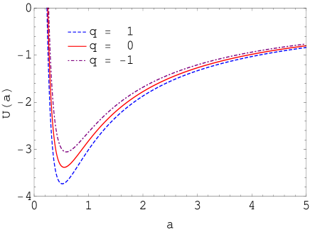
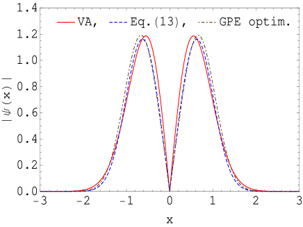
Figure 1: (Color online) Left panel: A molecular type potential associated with VA Eq. (10) for different strengths of the contact interaction. Right panel: The shape of a two-soliton molecule in a pure dipolar BEC with $N=2$, $q=0$, $g=20$ as predicted by VA with trial function (6) for $A=3.538$, $a=0.553$, $N=1.876$ (red solid line), by two anti-phase Gaussian functions with parameters given in Eq. (7) (blue dashed line), and found from numerical optimization procedure, applied to GPE (1) (brown dash-dot line). The minimum of the effective potential $U(a)$ is attained at $a_{0}=0.53$, and the equilibrium distance between center-of-mass positions of pulses predicted by Eq. (7) is $\Delta_{0}=4a_{0}/\sqrt{\pi}\simeq 1.2$, while the GPE optimization gives $\Delta_{0}\simeq 1.3$.

When solitons of the molecule are placed at their equilibrium positions, they stay motionless, as shown Fig. 2. If solitons are slightly displaced and released, they perform small amplitude oscillations around their stationary separation. The dynamics of the molecule strongly depends on the initial phase difference between solitons. In particular, even slight deviation from anti-phase configuration leads to periodic exchange of atoms between solitons. At larger deviation the soliton molecule does not form.

  

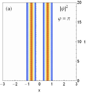
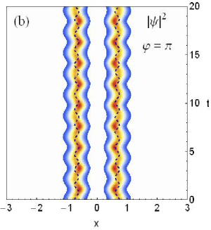
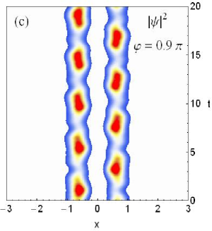
Figure 2: (Color online) (a) Stable propagation of a two-soliton molecule composed of two anti-phase ($\varphi=\pi$) Gaussian pulses with parameters $A_{0}=1.196$, $a_{0}=0.394$, placed at their equilibrium positions $x_{0}=\pm 0.657$. (b) When the solitons are slightly (by 20 %) displaced from equilibrium positions, they perform oscillations. Density plot $|\psi|^{2}$ is obtained by numerical solution of the GPE (1). Dashed line corresponds to calculations according to VA equation (10), which shows increasing phase shift with respect to GPE. (c) Periodic exchange of atoms between two solitons when the initial phase difference is slightly decreased.

The frequency of soliton oscillations near equilibrium state can be estimated from linearized version of Eq. (10)

$$\Omega_{0}^{2} = \frac{3}{a_{0}^{4}}-\frac{Nq}{2\sqrt{2\pi}a_{0}^{3}}\frac{\delta gN}{4\sqrt{2}a_{0}^{3}}\left[-15z_{0}^{2}\mathcal{U}\left(\frac{5}{2},0,z_{0}\right)+21z_{0}^{2}\mathcal{U}\left(\frac{5}{2},1,z_{0}\right)\right.$$ (11)

$$-\left.9z_{0}^{2}\mathcal{U}\left(\frac{5}{2},2,z_{0}\right)+20z_{0}\mathcal{U}\left(\frac{3}{2},-1,z_{0}\right)-28z_{0}\mathcal{U}\left(\frac{3}{2},0,z_{0}\right)+13z_{0}\mathcal{U}\left(\frac{3}{2},1,z_{0}\right)-2\mathcal{U}\left(\frac{1}{2},0,z_{0}\right)\right].$$

For the period of oscillations near the stationary separation we have $T_{VA}=2\pi/\Omega_{0}\simeq 1.54$. The prediction of VA is in qualitative agreement with the result of numerical simulation of the GPE, $T_{GPE}\simeq 2.2$ (see Fig. 2). In general, the VA provides fairly good description of the static and dynamic properties of the soliton molecule, while its waveform remains close to the selected trial function (6). The agreement between VA and GPE deteriorates at large separation between solitons, close to the dissociation point, when the trial function cannot be well approximated by two anti-phase Gaussian functions.

III Improving the shape of the soliton molecule by optimization procedure

The VA provides approximate waveform of a soliton molecule. When a trial function with parameters, defined by stationary solution of VA equation, is assigned as initial condition for the GPE, small amplitude oscillations of the molecule’s shape and separation between pulses is observed. This implies that soliton molecule is in its excited state.

For some precise parameter calculations, such as the binding energy of soliton molecules, a truly ground state should be employed. In Ref. golami2014 an optimization strategy to find the stationary shape of a soliton molecule in dispersion-managed optical fibers was proposed. Below we extend this approach for soliton molecules in dipolar BEC. It is based on the Nelder-Mead (NM) nonlinear optimization procedure nelder1965 , which seeks to minimize an objective (or cost) function

$$f=\frac{1}{N_{0}}\int\limits^{\infty}_{-\infty}(|\psi(x,0)|-|\psi(x,t_{1})|)^{2}\,dx,\qquad N_{0}=\int\limits^{\infty}_{-\infty}|\psi(x,0)|^{2}\,dx,$$ (12)

where

$$\psi(x,0)=A_{0}\left(\exp\left[-\frac{(x-x_{0})^{2}}{2a_{0}^{2}}\right]-\exp\left[-\frac{(x+x_{0})^{2}}{2a_{0}^{2}}\right]\right)$$ (13)

is the initial waveform, composed of two anti-phase Gaussian functions, separated by a distance $2\,x_{0}$, and $\psi(x,t_{1})$ is the result of evolution of $\psi(x,0)$ for some period of time $t=t_{1}$, according to GPE. Normalization factor $N_{0}$ in Eq. (12) is introduced to avoid trivial solutions, in particular corresponding to $x_{0}=0$. In general case minimization of the objective function can be performed with respect to variables $a_{0}$ and $x_{0}$, since the amplitude $A_{0}$ is fixed by the norm of the Gaussian. However, numerical experiments show that, VA predicted values of $a_{0}$ and $A_{0}$ for a single soliton are quite accurate, and minimization only with respect to pulse separation $x_{0}$ can produce stationary state of the molecule. The evolution time $t_{1}$ can be estimated as half period of oscillation for the molecule $t_{1}=\pi/\Omega_{0}$. Although the NM optimization procedure finds the minimum of the objective function (12) for Gaussian functions with broad range of parameters, the convergence rate can be improved by selecting the initial waveform close to the stationary state. The VA can provide the waveform which is close to the stationary state. We find stationary pulse separation $x_{0}$ and norm of the soliton molecule $N$ from NM optimization procedure. The obtained results were confirmed by alternative method of Luus-Jaakola lj1973 ; almarzoug2006 . Our preference of these optimization methods is motivated by several advantages, such as simplicity of programming (since calculation of function derivatives is not required), high convergence rate and reliability and effectiveness in locating the global minimum of the objective function.

IV Interaction potential and binding energy of soliton molecules

The binding energy of a soliton molecule $E_{b}$ can be defined as the amount of energy, which is required for the dissociation of the molecule into two separate individual free solitons, far away from each other. In numerical simulations using the GPE, the process of dissociation can be implemented by assigning an initial velocity to each soliton in opposite directions $\psi=\psi_{1}e^{ivx}+\psi_{2}e^{-ivx}$. If the velocity is smaller than some critical value $v<v_{cr}$, solitons perform oscillations around their stationary positions, otherwise the molecule disintegrates into individual solitons, travelling in opposite directions, as illustrated in Fig. 3.

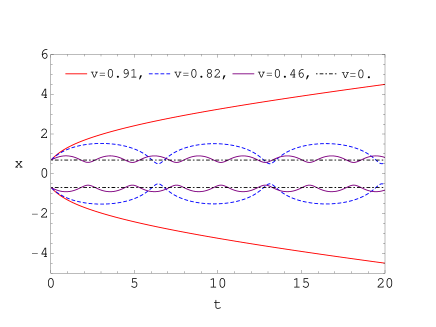
Figure 3: (Color online) Dynamics of center-of-masses of two solitons, forming the molecule, when the two solitons are set in motion with different velocities in opposite directions. When the velocity is less than critical $v<v_{cr}=0.91$, solitons perform oscillations near equilibrium positions. At critical velocity the molecule dissociates into freely moving individual solitons (red solid lines).

In a “particle in potential well” picture this situation corresponds to the escape of the particle from the potential well at critical kinetic energy. The critical velocity determines the binding energy of the molecule $E_{b}\sim v_{cr}^{2}/2$. Fig. 4 illustrates the potential of interactions between the two solitons, normalized to binding energy, as a function of distance between solitons in units of stationary separation $x_{0}$. To construct the potential $U(x)$ we assign velocity to solitons and determine the maximal and minimal value of the separation, which correspond to right and left classical turning points of the oscillating particle in the potential well. Repeating these calculations for velocities in the range $v\in[0,v_{cr}]$ we construct the potential, shown in the left panel of Fig. 4. As expected, the bigger norm $N$ (or number of atoms) of the molecule corresponds to stronger potential, connecting solitons.

  

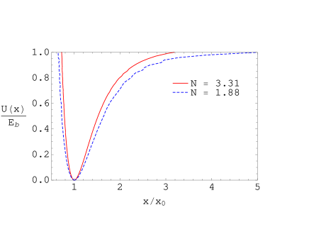
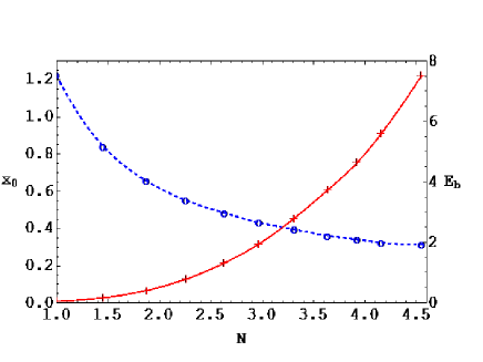
Figure 4: (Color online) Left panel: The potential of interaction between two solitons, retrieved from numerical GPE simulation, for two values of the molecule’s norm. Similarity with the VA predicted potential $U(a)$ in Fig. 1 is evident. Right panel: The stationary half separation between solitons of the molecule $x_{0}$ (blue dashed line) and its binding energy $E_{b}$ (red solid line) as a function of the molecule’s norm $N$. Symbols correspond to values found from numerical simulations of the GPE (1), and lines are interpolating curves for visual convenience.

The critical velocity $v_{cr}$, at which the molecule disintegrates into far separated individual solitons, is determined from GPE simulations, by setting in motion the two bound solitons in opposite directions, as shown in Fig. 4. In the experiment pushing the solitons in opposite directions can be realized by means of a laser beam, directed into the center of the molecule, as it was used to split the condensate in two halves nguyen2014 . The intensity of the laser beam can be varied to give desired initial velocity to solitons.

About the repulsive interaction between two anti-phase solitons the following comment is appropriate. As experimentally demonstrated in nguyen2014 and theoretically shown in rag2015 , two colliding wave packets exchange not only velocities (as classical particles do), but also their entire wave-functions (as quantum mechanical particles do via tunnel phenomenon). In our case of equal masses of two colliding solitons, the classical and quantum descriptions lead to the same result. Physically, the repulsive interaction of anti-phase matter wave solitons can be regarded as exchange of velocities of two colliding classical particles interacting via hard core potential.

V Numerical simulation of the two-soliton interactions

In order to study the character of interaction between two matter-wave solitons in numerical experiments we employ the idea similar to that used for optical solitons in fibers mitschke1987 . Initially at $t=0$, two solitons either in-phase $\phi=0$ or out-of-phase $\phi=\pi$, are created at some distance $\Delta_{0}$ from each-other. At later time $t=t_{1}>0$ the distance between solitons is measured again. If the solitons did not interact, the distance between them should not change with respect to its initial value $\Delta_{1}=\Delta_{0}$. If the interaction was attractive, the final measured distance should be less than the initial distance $\Delta_{1}<\Delta_{0}$. Finally if the interaction was repulsive, the final distance should be greater than the initial distance $\Delta_{1}>\Delta_{0}$. The numerical experiment consists in repeating the above procedure for different values of the initial distance $\Delta_{0}$, starting from sufficiently large separation, greatly exceeding the width of the soliton then reaching small distances when solitons start to overlap.

The result is presented in Fig. 5 as a plot of $\Delta_{1}$ (final separation) vs. $\Delta_{0}$ (initial separation). When the solitons, comprising the molecule, are out of phase ($\phi=\pi$) we see that at large separations the solitons do not interact ($\Delta_{1}\approx\Delta_{0}$, red curve is close to median), while at small distances they attract each other ($\Delta_{1}<\Delta_{0}$, red curve is below the median) until they reach a minimum (stationary) separation, where again $\Delta_{1}=\Delta_{0}$ (red dot on the median). When solitons are placed at even smaller distances, they repel each other ($\Delta_{1}>\Delta_{0}$, red curve is above the median). That is, the two-soliton molecule behaves like a diatomic molecule. For in-phase solitons ($\phi=0$) we see that solitons attract each other until their separation becomes comparable to the width of the soliton, then merge forming a wave packet, whose shape strongly oscillates.

  

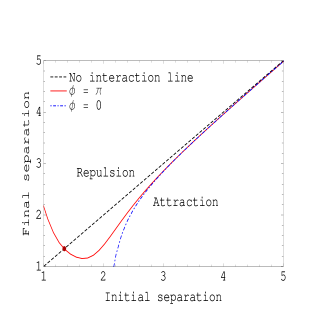
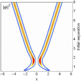
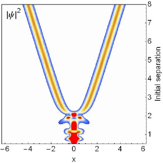
Figure 5: (Color online) Left panel: The character of soliton interactions for anti-phase and in-phase solitons. Anti-phase solitons attract each-other at large separations and repel at small separations (red solid line). There exists a stationary separation, shown by a red dot, where attraction changes to repulsion. In-phase solitons always attract and collide (blue dashed line). Middle panel: Anti-phase solitons can form a stable soliton molecule at appropriate initial separation $\Delta_{0}\simeq 1.3$. Right panel: In-phase solitons always collide and do not form stable bound state.

The numerical simulations are performed using realistic values of atom numbers and interaction parameters in ¹⁶⁴Dy for which $m=2.7\times 10^{-25}$ kg, $d=10\,\mu_{B}=9.27\times 10^{-23}$ A m², $a_{d}=\mu_{0}d^{2}m/(12\pi\hbar^{2})\simeq 7\times 10^{-9}$ m. The frequency of radial confinement $\omega_{\bot}=2\pi\times 62$ Hz provides radial oscillator length $l_{0}\simeq 1\,\mu$m and unit of time $t_{0}=2.6$ ms. For parameter values $g_{0}=20$ and $N=2$ used in numerical simulations we obtain the number of atoms in a two-soliton molecule ${\cal N}=g_{0}Nl_{0}/(2a_{d})\simeq 3000$. The total number of atoms in the ¹⁶⁴Dy condensate was ${\cal N}=15000$ lu2011 .

VI conclusions

We have studied the interaction between two bright solitons in a dipolar BEC and found the conditions when they form a stable bound state. It was revealed by numerical simulations of the governing nonlocal GPE and corresponding variational analysis, that two anti-phase solitons in dipolar condensates behave similarly to a diatomic molecule. Namely, they attract each-other at large separation and repel each-other at small separation. There exists a particular distance at which the two solitons remain motionless in their stationary state. Solitons in a weakly perturbed molecule perform small amplitude oscillations near the equilibrium position, the frequency of which is predicted quite accurately by the developed model. Two in-phase solitons when placed close to each-other always collide and do not form the bound state. The obtained results can be useful in further studies of the properties of multi-soliton bound states in dipolar BEC.

References

- (1) N. J. Zabusky and M. D. Kruskal, Phys. Rev. Lett. 15, 240 (1965).
- (2) J. H. V. Nguyen, P. Dyke, De Luo, B. A. Malomed and R. G. Hulet, Nature Phys. 10, 918 (2014).
- (3) A. Hasegawa and Y. Kodama, Solitons in optical communications (Clarendon Press, Oxford, 1995).
- (4) J. P. Gordon, Opt. Lett., 8, 596 (1983).
- (5) F. Mitschke and L. Mollenauer, Opt. Lett. 12, 355 (1987).
- (6) Y. Kodama and K. Nozaki, Opt. Lett. 12, 1038 (1987); K. Smith and L. F. Mollenauer, Opt. Lett. 14, 1284 (1989).
- (7) L. F. Mollenauer and J. P. Gordon, Solitons in Optical Fibers: Fundamentals and Applications (Academic Press, San Diego, 2006).
- (8) G. I. Stegeman and M. Segev, Science, 286, 1518 (1999).
- (9) K. E. Lonngren, Plasma Phys. 25, 943 (1983).
- (10) C. Rotschild, B. Alfassi, O. Cohen and M. Segev, Nature Phys. 2, 769 (2006); J. K. Jang, M. Erkintalo, S. G. Murdoch and S. Coen, Nature Photon. 7, 657 (2013).
- (11) A. D. Cronin, J. Schmiedmayer, and D. E. Pritchard, Rev. Mod. Phys. 81, 1051 (2009); T. Berrada, S. van Frank, R. Bücker, T. Schumm, J. -F. Schaff, and J. Schmiedmayer, Nature Commun. 4, 2077 (2013).
- (12) G. D. McDonald, C. C. N. Kuhn, K. S. Hardman, S. Bennetts, P. J. Everitt, P. A. Altin, J. E. Debs, J. D. Close, and N. P. Robins, Phys. Rev. Lett. 113, 013002 (2014).
- (13) J. Cuevas, P. G. Kevrekidis, B. A. Malomed, P. Dyke and R. G. Hulet, New J. Phys. 15, 063006 (2013); J. Polo and V. Ahufinger, Phys. Rev. A 88, 053628 (2013); H. Michinel, A. Paredes, M. M. Valado, and D. Feijoo, Phys. Rev. A 86, 013620 (2012).
- (14) S. Burger et al., Phys. Rev. Lett. 83, 5198 (1999); J. Denschlag et al., Science 287, 97 (2000); K. E. Strecker et al., Nature 417, 150 (2002); L. Khaykovich et al., Science 296, 1290 (2002); S. L. Cornish et al., Phys. Rev. Lett. 96, 170401 (2006); C. Becker et al., Nat. Phys. 4, 496 (2008); C. Hamner et al., Phys. Rev. Lett. 106, 065302 (2011).
- (15) A. L. Marchant, T. P. Billam, T. P. Wiles, M. M. H. Yu, S. A. Gardiner, and S. L. Cornish, Nat. Commun. 4, 1865 (2013).
- (16) P. Medley, M. A. Minar, N. C. Cizek, D. Berryrieser, and M. A. Kasevich, Phys. Rev. Lett. 112, 060401 (2014).
- (17) U. Al Khawaja, H. T. C. Stoof, R. G. Hulet, K. E. Strecker, and G. B. Partridge, Phys. Rev. Lett. 89, 200404 (2002).
- (18) C. C. Bradley, C. A. Sackett, and R. G. Hulet, Phys. Rev. Lett. 78, 985 (1997).
- (19) A. Griesmaier, J. Werner, S. Hensler, J. Stuhler and T. Pfau, Phys. Rev. Lett. 94, 160401 (2005).
- (20) M. Lu, N. Q. Burdick, S. H. Youn, and B. L. Lev, Phys. Rev. Lett. 107, 190401 (2011).
- (21) K. Aikawa, A. Frisch, M. Mark, S. Baier, A. Rietzler, R. Grimm, and F. Ferlaino, Phys. Rev. Lett. 108, 210401 (2012).
- (22) M. Stratmann, T. Pagel, and F. Mitschke, Phys. Rev. Lett. 95, 143902 (2005); P. Rohrmann, A. Hause, and F. Mitschke, Sci. Rep. 2, 866 (2012); P. Rohrmann, A. Hause, and F. Mitschke, Phys. Rev. A 87, 043834 (2013); A. Hause and F. Mitschke, Phys. Rev. A 88, 063843 (2013).
- (23) R. Nath, P. Pedri, and L. Santos, Phys. Rev. A 76, 013606 (2007).
- (24) A. I. Yakimenko, V. M. Lashkin, and O. O. Prikhodko, Phys. Rev. E 73, 066605 (2006); V. M. Lashkin, A. I. Yakimenko, O. O. Prikhodko, Phys. Lett. A 366, 422 (2007).
- (25) B. P. Anderson and P. Meystre, Cont. Phys., 44, 473 (2003).
- (26) J. Cuevas, Boris A. Malomed, P. G. Kevrekidis, and D. J. Frantzeskakis, Phys. Rev. A 79, 053608 (2009).
- (27) F. Kh. Abdullaev and V. A. Brazhnyi, J. Phys. B: At. Mol. Opt. Phys. 45, 085301 (2012).
- (28) S. Sinha and L. Santos, Phys. Rev. Lett. 99, 140406 (2007).
- (29) C. Pare and P.-A. Belanger, Opt. Commun. 168, 103 (1999); B.-F. Feng and B. A. Malomed, Opt. Commun. 229, 173 (2004); S. M. Alamoudi, U. Al Khawaja, and B. B. Baizakov, Phys. Rev. A 89, 053817 (2014).
- (30) M. Abramowitz and I. A. Stegun, Handbook of Mathematical Functions, (National Bureau of Standards, Washington, 1964).
- (31) S. Gholami, Ph. Rohrmann, A. Hause and F. Mitschke, Appl. Phys. B 116, 43 (2014).
- (32) J. A. Nelder and R. Mead, Comput. J. 7, 308 (1965).
- (33) R. Luus and T. H. I Jaakola, AIChE J., 19 760 (1973).
- (34) S. M. Al-Marzoug, R. J. W. Hodgson, Opt. Commun. 265, 234 (2006).
- (35) H. S. Rag and J. Gea-Banacloche, Am. J. Phys. 83, 305 (2015).