Geometric elements and classification of quadrics in rational Bézier form

Abstract

In this paper we classify and derive closed formulas for geometric elements of quadrics in rational Bézier triangular form (such as the center, the conic at infinity, the vertex and the axis of paraboloids and the principal planes), using just the control vertices and the weights for the quadric patch. The results are extended also to quadric tensor product patches. Our results rely on using techniques from projective algebraic geometry to find suitable bilinear forms for the quadric in a coordinate-free fashion, considering a pencil of quadrics that are tangent to the given quadric along a conic. Most of the information about the quadric is encoded in one coefficient, involving the weights of the patch, which allows us to tell apart oval from ruled quadrics. This coefficient is also relevant to determine the affine type of the quadric. Spheres and quadrics of revolution are characterised within this framework.

1 Introduction

One of the reasons for extending the framework of surfaces used in CAD from polynomial or piecewise polynomial surfaces to rational ones is the inclusion of quadrics in an exact fashion, since quadric surfaces such as spheres, cones, cylinders, paraboloids are commonly used in engineering and in architecture [1].

There are mainly two ways of implementing surfaces in CAD: tensor product patches and Bézier triangles [2]. The former ones are the most common, but the latter have applications in animation and finite element theory due to the flexibility of triangles, compared to quadrilaterals, for constructing surfaces and adapting to different topologies without producing singularities.

Whereas rational quadratic curves are conics, we have a different situation when we go to surfaces. On one hand, not every quadric triangular patch can be represented as a rational quadratic Bézier triangle. On the other hand, rational quadratic Bézier triangles are in general quartic surfaces [3] and only in some cases quadric patches are obtained [4].

Quadric triangular patches have been studied from many points of view. [5] describes a method for constructing quadric patches grounded on a quadratic Bézier control polyhedron. [6] and [7] use an algebraic approach to construct curves and surfaces on quadrics. [8] classifies quadratically parametrised surfaces and studies their geometry. [9] provides a thorough classification of rational quadratic triangles. [10] provides an algorithm for checking whether a rational Bézier triangle belongs to a quadric and classifying it. This solution is shown in [11] to be one of fifteen possibilities, with different numerical conditioning. In [12] the algorithm is used to obtain the axes of the quadric. [13] provides a tool for constructing rational quadratic patches on non-degenerate quadrics. Three corner points and three weights are used as shape parameters in [14] to design quadric surface patches. In [15] the shape parameters are three points and the normal vectors at them.

In this paper we draw geometric information from rational Bézier quadric triangles and tensor product patches. We classify them and calculate their geometric elements in closed form, using just the control net and the weights of the patch, as it is done for conics in [16]. One of the reasons for doing this is that closed formulas for geometric elements of a quadric can be of great help for designing with them.

With this goal in mind, we derive bilinear forms for the quadrics, both in point and tangential form in a coordinate-free fashion, using techniques borrowed from algebraic projective geometry, such as the use of pencils of quadrics, which have also been used in [14, 15, 17]. Using linear forms with clear geometric meaning (tangent planes, planes containing boundary conics…) instead of, for instance, cartesian coordinates, allows us to find a closed form for the implicit equation of these quadrics in terms of their weights, their tangent planes and the plane spanned by the corner vertices of the patch. The major originality and advantage of our formulation is the use of only geometric information about the patch, avoiding the use of coordinate expressions as an intermediate step. In fact, most of the relevant geometric information of the surface which is necessary for its classification is comprised in a single coefficient, the parameter of the pencil of quadrics, which depends on the weights of the patch.

The coordinate-free bilinear forms for the quadrics enable the derivation of closed formulas for several geometric elements (center of the quadrics, bilinear forms for the conic at infinity, diametral planes) calculated in terms of weights and vertices. To our knowledge, such closed formulas have not been produced before. Similarly, linear forms for principal planes are obtained up to solving a cubic equation. The degeneracy of the solutions of this equation allows us to identify quadrics of revolution and spheres.

Finally, the previous results for triangular quadric patches can be extended to rational biquadratic quadric patches using the tangent planes at three corners of the boundary of the tensor product patch.

This paper is organised as follows: We revisit rational Bézier triangular patches and the characterisation of quadric patches in Section 2. In Section 3 we construct the pencil of quadrics, in point and in tangential form, which are tangent to our quadric at the conic through the three corner vertices of the patch and fix the only free parameter in terms of the weights of the quadric. This provides us bilinear forms for the quadrics and hence implicit equations. A coordinate-free expression for the center of the quadric is obtained in Section 4 as a barycentric combination of the corner vertices of the patch and the intersection of their tangent planes. It is used to tell paraboloids from centered quadrics. In Section 5 we calculate a bilinear form for the conic at infinity, which is useful for determining the affine type of the quadric. Section 6 is devoted to degenerate quadrics. With this information we provide in Section 7 a way to classify quadric patches using the signature of the bilinear form, the center and the bounding conic arcs. We introduce the scalar product in Section 8 in order to calculate Euclidean geometric elements such as principal planes and axes of quadrics and vertices of paraboloids. This allows us to characterise spheres and quadrics of revolution. In Section 9 we show several examples of application of our results. We show how to extend our results to quadric tensor product patches in Section 10. A final section of conclusions is included.

2 Quadratic rational Bézier triangular patches

Rational Bézier triangular patches of degree $n$ are defined using trivariate Bernstein polynomials of degree $n$ in parameters $u,v,w$,

$$B^{n}_{ijk}(u,v,w)=\frac{n!}{i!j!k!}u^{i}v^{j}w^{k},\quad i+j+k=n,$$

$$c(u,v,w)=\frac{\displaystyle\sum_{i+j+k=n}\omega_{ijk}c_{ijk}B^{n}_{ijk}(u,v,w)}{\displaystyle\sum_{i+j+k=n}\omega_{ijk}B^{n}_{ijk}(u,v,w)},$$ (1)

such that $u+v+w=1$, $u,v,w\in[0,1]$, where the coefficients $c_{ijk}$ are the control points for the surface and $\omega_{ijk}$ are their corrresponding weights.

The surface patch is bounded by three rational Bézier curves of degree $n$, which are obtained by fixing $u=0$, $v=0$, $w=0$. Their respective control points and weights are respectively the ones with index $i=0$, $j=0$, $k=0$.

We are interested in the special case of quadratic surfaces. In this case the control net and the matrix of weights are

$$\left[\begin{array}[]{c}c_{002}\hskip 5.69046ptc_{011}\hskip 5.69046ptc_{020}\\ c_{101}\hskip 5.69046ptc_{110}\\ c_{200}\end{array}\right],\qquad\left[\begin{array}[]{c}\omega_{002}\hskip 5.69046pt\omega_{011}\hskip 5.69046pt\omega_{020}\\ \omega_{101}\hskip 5.69046pt\omega_{110}\\ \omega_{200}\end{array}\right],$$ (2)

and the surface patch is completely determined by the three boundary conic curves:

The conic at $u=0$ has control points $\{c_{002},c_{011},c_{020}\}$ and weights $\{\omega_{002},\omega_{011},\omega_{020}\}$, the one at $v=0$ has control points $\{c_{002},c_{101},c_{200}\}$ and weights $\{\omega_{002},\omega_{101},\omega_{200}\}$, and the one at $w=0$ has control points $\{c_{020},c_{110},c_{200}\}$ and weights $\{\omega_{020},\omega_{110},\omega_{200}\}$. We just consider the case of non-degenerate boundary curves. We name the planes where such conics are located respectively as $u,v,w$.

Quadratic rational Bézier triangular surfaces comprise quadrics as a subcase, but in general they are quartic surfaces named Steiner surfaces [3]. On the contrary, not every quadric patch bounded by three arcs can be parametrised as a quadratic rational Bézier triangle. According to [4]:

• If the Steiner surface is a non-degenerate quadric, the three conic boundary curves meet at a point $S$ and their respective tangent vectors at $S$ define a plane.

• If the three conic boundary curves meet at a point $S$ and their respective tangent vectors at $S$ define a plane, the Steiner surface is a quadric patch.

• If there are three alligned points, one on each boundary conic curve, and the tangent plane to the surface is the same for all three points, the Steiner surface is a degenerate quadric patch.

The last case just implies that the quadric (cylinder or cone) is ruled and the three points lie on the same ruling.

We are considering Steiner surfaces with such a point $S$. This case comprises non-degenerate quadrics. Since $S$ belongs to the three boundary conics, there are values $u_{s},v_{s},w_{s}$ of the parameters such that

$$S = \frac{\displaystyle\sum_{j=0}^{2}\omega_{0j2-j}c_{0j2-j}B^{2}_{j}(v_{s})}{\displaystyle\sum_{j=0}^{2}\omega_{0j2-j}B^{2}_{j}(v_{s})}=\frac{\displaystyle\sum_{i=0}^{2}\omega_{i2-i0}c_{i2-i0}B^{2}_{i}(u_{s})}{\displaystyle\sum_{i=0}^{2}\omega_{i2-i0}B^{2}_{i}(u_{s})}$$

$$= \frac{\displaystyle\sum_{k=0}^{2}\omega_{2-k0k}c_{2-k0k}B^{2}_{k}(w_{s})}{\displaystyle\sum_{k=0}^{2}\omega_{2-k0k}B^{2}_{k}(w_{s})},$$

where we have introduced quadratic Bernstein polynomials,

$$B^{2}_{0}(t)=(1-t)^{2},\quad B^{2}_{1}(t)=2t(1-t),\quad B^{2}_{2}(t)=t^{2}.$$

However, since the set of weights of rational Bézier curves is unique up to Möbius transformations [18] of the parameter, we can use this freedom to set $u_{s}$, $v_{s}$, $w_{s}$ at infinity. It is a simple exercise to check that this is possible if and only if the tangent vectors at $S$ are coplanar [19]. Hence, this choice is not a restriction.

From now on we assume that the set of weights for the surface fulfills this condition and therefore we may write $S$ in three different forms as

$$S = \frac{\omega_{002}c_{002}-2\omega_{011}c_{011}+\omega_{020}c_{020}}{\omega_{u}}$$ (3)

$$= \frac{\omega_{002}c_{002}-2\omega_{101}c_{101}+\omega_{200}c_{200}}{\omega_{v}}$$

$$= \frac{\omega_{200}c_{200}-2\omega_{110}c_{110}+\omega_{020}c_{020}}{\omega_{w}},$$

where $\omega_{u},\omega_{v},\omega_{w}$ guarantee that these are barycentric combinations,

$$\omega_{u}=\omega_{002}-2\omega_{011}+\omega_{020},\ \omega_{v}=\omega_{002}-2\omega_{101}+\omega_{200},$$

$$\omega_{w}=\omega_{200}-2\omega_{110}+\omega_{020},$$

if $S$ is a proper point. If $S$ is point at infinity, the coefficients $\omega_{u},\omega_{v},\omega_{w}$ are chosen in order to have the same vector as representantive for $S$ on the three boundary curves.

3 Pencils of Steiner quadrics

In order to obtain a bilinear form for the quadric, we describe the pencil of quadrics which are tangent to our quadric at the conic on the plane $t$ defined by the points at the corners of the surface patch, $P=c_{002}$, $Q=c_{020}$, $R=c_{200}$. This pencil of quadrics has been used also in [14, 15, 17].

To this aim, we just need two quadrics belonging to the pencil [20], which can be degenerate.

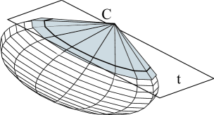
Figure 1: Tangent cone to a quadric along a conic on a plane $t$

For instance, we can take the cone $C$ tangent to our quadric along the conic on $t$ and the double plane $t$ (see Fig. 1). Hence, the bilinear form for this pencil of quadrics is just $C+\lambda t^{2}$, using the same letter for a surface and its form. Finally, we can determine our quadric just using the existence of point $S$,

$$C(S)+\lambda t(S)^{2}=0.$$

We just have then to provide a bilinear form for the cone $C$. Since $\lambda=-C(S)/t(S)^{2}$, we notice that the sign of $\lambda$ depends on whether $S$ lies in or out of the cone $C$.

It will be useful to start with the bilinear form for the conic on $t$ (see Fig. 2). In this figure $u,v,w$ are the straight lines which are respectively the intersections of the planes $u,v,w$ (where the boundary conics lie) with the plane $t$.

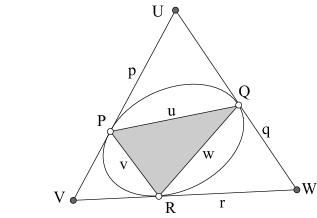
Figure 2: Conic circumscribed by a triangle

We use the same letter for a point (uppercase) and its polar line (lower case). If a point $A$ lies on the conic, its polar line is the tangent $a$ to the conic at such point. Hence, $p$, $q$, $r$ are respectively the tangent lines to the conic at $P$, $Q$, $R$ (see Fig. 3). We shall use the same letters $p,q,r$ also for the tangent planes at $P,Q,R$.

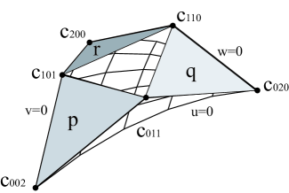
Figure 3: Tangent planes $p,q,r$

On the other hand, the polar line to a point $A$ not on the conic is the line $a$ linking the tangency points of the tangent lines to the conic drawn from $A$. Hence, $u$, $v$, $w$ are the polar lines to the vertices of the circumscribed triangle $U$, $V$, $W$.

The pencil of conics circumscribed by the triangle defined by the lines $p$, $q$, $r$ is easily described in tangential form. The bilinear form for this pencil is just

$$\alpha UV+\beta UW+\gamma VW,$$

with coefficients $\alpha$, $\beta$, $\gamma$. It is easy to check that this form vanishes on $p$, $q$, $r$, since

$$p(U)=0=p(V),\ q(U)=0=q(W),\ r(V)=0=r(W).$$

But, for our purposes, we require the point bilinear form for the conic. Referred to the lines $r$, $q$, $p$, which form a dual reference to the one formed by $U$, $V$, $W$, provided that their linear forms satisfy

$$p(W)=1,\quad q(V)=1,\quad r(U)=1,$$ (4)

the matrix of this point bilinear form is the inverse of the one for the tangential bilinear form,

$$\left(\begin{array}[]{ccc}0&\alpha&\beta\\ \alpha&0&\gamma\\ \beta&\gamma&0\end{array}\right)^{-1}=-\frac{1}{2\alpha\beta\gamma}\left(\begin{array}[]{ccc}\gamma^{2}&-\beta\gamma&-\alpha\gamma\\ \ -\beta\gamma&\beta^{2}&-\alpha\beta\\ -\alpha\gamma&-\alpha\beta&\alpha^{2}\end{array}\right),$$

and hence such a bilinear form is

$$\alpha^{2}p^{2}-2\alpha\beta pq-2\alpha\gamma pr+\beta^{2}q^{2}-2\beta\gamma qr+\gamma^{2}r^{2}.$$

In order to determine the coefficients $\alpha,\beta,\gamma$, it is useful to take into account that (3) provides relations between values of the linear forms for $p,q,r$,

$$\frac{\omega_{020}}{\omega_{u}}p(Q)=p(S)=\frac{\omega_{200}}{\omega_{v}}p(R),$$

$$\frac{\omega_{200}}{\omega_{w}}q(R)=q(S)=\frac{\omega_{002}}{\omega_{u}}q(P),$$

$$\frac{\omega_{002}}{\omega_{v}}r(P)=r(S)=\frac{\omega_{020}}{\omega_{w}}r(Q),$$

which can be used to write $U,V,W$ in terms of $P,Q,R$,

$$U=\frac{\omega_{002}\omega_{w}P+\omega_{020}\omega_{v}Q-\omega_{200}\omega_{u}R}{\Omega_{U}},$$

$$V=\frac{\omega_{002}\omega_{w}P-\omega_{020}\omega_{v}Q+\omega_{200}\omega_{u}R}{\Omega_{V}},$$

$$W=\frac{-\omega_{002}\omega_{w}P+\omega_{020}\omega_{v}Q+\omega_{200}\omega_{u}R}{\Omega_{W}},$$ (5)

or, conversely,

$$P=\frac{\Omega_{U}U+\Omega_{V}V}{2\omega_{002}\omega_{w}},Q=\frac{\Omega_{W}W+\Omega_{U}U}{2\omega_{020}\omega_{v}},R=\frac{\Omega_{V}V+\Omega_{W}W}{2\omega_{200}\omega_{u}},$$

where the normalisation denominators are

$$\Omega_{U}=\omega_{002}\omega_{w}+\omega_{020}\omega_{v}-\omega_{200}\omega_{u},$$

$$\Omega_{V}=\omega_{002}\omega_{w}-\omega_{020}\omega_{v}+\omega_{200}\omega_{u},$$

$$\Omega_{W}=-\omega_{002}\omega_{w}+\omega_{020}\omega_{v}+\omega_{200}\omega_{u},$$ (6)

provided that $U,V,W$ are proper points. If one of these points goes to infinity, the respective denominator is taken to be one. The interpretation of these coefficients as weights for $U,V,W$ on the conic on $t$ is discussed in Section 6.

Finally, the normalisation condition (4) allows us to fix the linear forms for $p,q,r$ since

$$p(W)=\displaystyle\frac{2\omega_{u}\omega_{v}}{\Omega_{W}}p(S),\qquad q(V)=\frac{2\omega_{u}\omega_{w}}{\Omega_{V}}q(S),$$

$$r(U)=\displaystyle\frac{2\omega_{v}\omega_{w}}{\Omega_{U}}r(S).$$ (7)

Since we require that points $P$, $Q$, $R$ lie on the conic,

$$\beta q(P)=\gamma r(P),\quad\alpha p(Q)=\gamma r(Q),\quad\alpha p(R)=\beta q(R),$$

we identify the coefficients of the bilinear form,

$$\alpha=\frac{1}{\Omega_{W}},\quad\beta=\frac{1}{\Omega_{V}},\quad\gamma=\frac{1}{\Omega_{U}},$$

up to a common factor.

Hence, a bilinear form for the conic on $t$ is

$$\frac{p^{2}}{\Omega_{W}^{2}}+\frac{q^{2}}{\Omega_{V}^{2}}+\frac{r^{2}}{\Omega_{U}^{2}}-\frac{2pq}{\Omega_{W}\Omega_{V}}-\frac{2pr}{\Omega_{W}\Omega_{U}}-\frac{2qr}{\Omega_{V}\Omega_{U}}$$ (8)

and, in tangential form,

$$\Omega_{U}\Omega_{V}UV+\Omega_{U}\Omega_{W}UW+\Omega_{V}\Omega_{W}VW.$$ (9)

The terms of the bilinear form can be factored as

$$\left(\frac{p}{\Omega_{W}}-\frac{q}{\Omega_{V}}-\frac{r}{\Omega_{U}}\right)^{2}+\left(\frac{q}{\Omega_{V}}-\frac{r}{\Omega_{U}}\right)^{2}-\left(\frac{q}{\Omega_{V}}+\frac{r}{\Omega_{U}}\right)^{2},$$

and thereby it has signature $(++-)$ regardless of the values of the coefficients.

We move now back from plane to space: If $p$, $q$, $r$ are the tangent planes to the quadric at $P$, $Q$, $R$, the bilinear form (8) describes a degenerate quadric of signature $(++-\,0)$ which contains the conic on $t$ and it is tangent to our quadric along it. Since the rank of the bilinear form is three, it is a cone (or a cylinder, if the intersection point of $p$, $q$, $r$ goes to infinity), since these are the only non-plane degenerate quadrics. Hence, it is the cone we are looking for.

The bilinear form for the pencil of quadrics referred to the planes $r,q,p,t$,

$$\frac{p^{2}}{\Omega_{W}^{2}}+\frac{q^{2}}{\Omega_{V}^{2}}+\frac{r^{2}}{\Omega_{U}^{2}}-\frac{2pq}{\Omega_{W}\Omega_{V}}-\frac{2pr}{\Omega_{W}\Omega_{U}}-\frac{2qr}{\Omega_{V}\Omega_{U}}+\lambda t^{2},$$

produces a bilinear form for our quadric if $\lambda=-C(S)/t(S)^{2}$.

We see that the sign of $\lambda$ determines the signature of the bilinear form, defined as the difference between the number of its positive and negative eigenvalues. This is relevant since ruled quadrics have null signature, $(++--)$ and oval quadrics have signature two $(++-+)$. This is useful to classify the quadric.

In tangential form referred to the points $U,V,W,T$, the bilinear form for the quadric is

$$\Omega_{U}\Omega_{V}UV+\Omega_{U}\Omega_{W}UW+\Omega_{V}\Omega_{W}VW-\frac{T^{2}}{\lambda},$$

if $t(T)=1$, where $T$ is the intersection point of the planes $p,q,r$, that is, the vertex of the cone $C$.

With this information we can write $T$ as

$$T\!\!\! = \!\!\!\frac{\omega_{002}\omega_{w}(\omega_{u}+\omega_{v}-\omega_{w})P+\omega_{020}\omega_{v}(\omega_{u}-\omega_{v}+\omega_{w})Q}{\epsilon_{U}\Omega_{U}\omega_{u}+\epsilon_{V}\Omega_{V}\omega_{v}+\epsilon_{W}\Omega_{W}\omega_{w}-2\epsilon_{S}\omega_{u}\omega_{v}\omega_{w}}$$ (10)

$$+ \frac{\omega_{200}\omega_{u}(-\omega_{u}+\omega_{v}+\omega_{w})R-2\omega_{u}\omega_{v}\omega_{w}S}{\epsilon_{U}\Omega_{U}\omega_{u}+\epsilon_{V}\Omega_{V}\omega_{v}+\epsilon_{W}\Omega_{W}\omega_{w}-2\epsilon_{S}\omega_{u}\omega_{v}\omega_{w}},$$

or alternatively,

$$S\!\!\! = \!\!\!\frac{\Omega_{U}}{2\omega_{v}\omega_{w}}U+\frac{\Omega_{V}}{2\omega_{u}\omega_{w}}V+\frac{\Omega_{W}}{2\omega_{u}\omega_{v}}W+$$

$$+ \frac{2\epsilon_{S}\omega_{u}\omega_{v}\omega_{w}-\epsilon_{U}\Omega_{U}\omega_{u}-\epsilon_{V}\Omega_{V}\omega_{v}-\epsilon_{W}\Omega_{W}\omega_{w}}{2\omega_{u}\omega_{v}\omega_{w}}T,$$

where $\epsilon_{A}$ takes the value one if the corresponding point $A$ is proper or zero if it is a point at infinity.

Now we can compute $\lambda$ and determine the quadric:

Theorem 1

A rational triangular quadratic patch with control net $\{c_{002},c_{011},c_{020},c_{101},c_{110},c_{200}\}$ and weights $\{\omega_{002},\omega_{011},\omega_{020},\omega_{101},\omega_{110},\omega_{200}\}$, such that the three boundary conics meet at a point $S$, which is written as in (3), is a quadric with bilinear form

$$\mathcal{Q}=\frac{p^{2}}{\Omega_{W}^{2}}+\frac{q^{2}}{\Omega_{V}^{2}}+\frac{r^{2}}{\Omega_{U}^{2}}-\frac{2pq}{\Omega_{W}\Omega_{V}}-\frac{2pr}{\Omega_{W}\Omega_{U}}-\frac{2qr}{\Omega_{V}\Omega_{U}}+\lambda t^{2},\$$ (11)

where $t$ is the linear form of the plane containing $c_{002},c_{020},c_{200}$, $p$ is the linear form of the plane containing $c_{002}$, $c_{011}$, $c_{101}$, $q$ is the linear form of the plane containing $c_{020}$, $c_{011}$, $c_{110}$ and $r$ is the linear form of the plane containing $c_{200}$, $c_{101}$, $c_{110}$ which satisfy

$$p(W)=1,\quad q(V)=1,\quad r(U)=1,\quad t(T)=1,$$

at the points $U$ (intersection of the planes $p,q,t$), $V$ (intersection of the planes $p,r,t$) and $W$ (intersection of the planes $q,r,t$) given by (3) and the point $T$ (intersection of the planes $p,q,r$), given by (10).

The coefficients are given in (3) except for $\lambda$,

$$\lambda=-\frac{\omega_{u}^{2}+\omega_{v}^{2}+\omega_{w}^{2}-2\omega_{u}\omega_{v}-2\omega_{v}\omega_{w}-2\omega_{w}\omega_{u}}{(2\epsilon_{S}\omega_{u}\omega_{v}\omega_{w}-\epsilon_{U}\Omega_{U}\omega_{u}-\epsilon_{V}\Omega_{V}\omega_{v}-\epsilon_{W}\Omega_{W}\omega_{w})^{2}},$$ (12)

and the tangential bilinear form for the quadric is

$$\tilde{\mathcal{Q}}=\Omega_{U}\Omega_{V}UV+\Omega_{U}\Omega_{W}UW+\Omega_{V}\Omega_{W}VW-\frac{T^{2}}{\lambda},$$ (13)

Furthermore, for $\lambda>0$ the quadric is oval and for $\lambda<0$ the quadric is ruled.

The expression we have obtained for the bilinear form of the quadric has the advantage of encoding most of the information about the surface in just the coefficient $\lambda$ for $t^{2}$.

This result provides a procedure for computing a bilinear form, and hence the implicit equation, for a non-degenerate Steiner quadric patch in a coordinate-free fashion using just the vertices of the control net and their respective weights:

1. Obtain $S$ as intersection of the planes $u,v,w$.

2. Compute the normalised linear forms for the planes $t,p,q,r$.

3. Obtain an equivalent list of weights fulfilling (3).

4. Use Theorem 1 to obtain the bilinear form $\mathcal{Q}$ for the quadric patch.

5. The implicit equation for the quadric patch is then $\mathcal{Q}(X,X)=0$.

4 Center of a quadric

The bilinear form for the quadric provides a way to obtain its center $Z$ as the pole of the plane $z$ at infinity. Since the plane at infinity is formed by vectors, we may write its elements as barycentric combinations

$$aU+bV+cW+dT,\qquad a+b+c+d=0.$$

We have to consider the possibility of having any of the points of the reference at infinity. In such case, the null sum is restricted to proper points,

$$aU+bV+cW+dT,\quad\epsilon_{U}a+\epsilon_{V}b+\epsilon_{W}c+\epsilon_{T}d=0.$$ (14)

Hence, a linear form for the plane at infinity in this reference is just

$$z=\epsilon_{W}p+\epsilon_{V}q+\epsilon_{U}r+\epsilon_{T}t.$$ (15)

The pole of this plane,

$$\tilde{\mathcal{Q}}(z) = \epsilon_{W}\Omega_{W}(\Omega_{U}U+\Omega_{V}V)+\epsilon_{V}\Omega_{V}(\Omega_{W}W+\Omega_{U}U)$$ (16)

$$+ \epsilon_{U}\Omega_{U}(\Omega_{V}V+\Omega_{W}W)-\frac{2\epsilon_{T}}{\lambda}T,$$

can be written in a simpler way in terms of $P,Q,R,T$ in order to produce an expression for the center of the quadric,

$$Z = \frac{\epsilon_{W}\Omega_{W}\omega_{w}\omega_{002}P+\epsilon_{V}\Omega_{V}\omega_{v}\omega_{020}Q+\epsilon_{U}\Omega_{U}\omega_{u}\omega_{200}R}{\Omega_{Z}}$$ (17)

$$- \frac{\epsilon_{T}}{\lambda\Omega_{Z}}T,\$$

where the denominator $\Omega_{Z}$ is one if the center is a point at infinity or, if it is a proper point,

$$\Omega_{Z}=\tilde{\Omega}_{W}\omega_{w}\omega_{002}+\tilde{\Omega}_{V}\omega_{v}\omega_{020}+\tilde{\Omega}_{U}\omega_{u}\omega_{200}-\frac{\epsilon_{T}}{\lambda},\$$ (18)

and we have introduced for simplicity,

$$\tilde{\Omega}_{U}=\epsilon_{U}\Omega_{U},\quad\tilde{\Omega}_{V}=\epsilon_{V}\Omega_{V},\quad\tilde{\Omega}_{W}=\epsilon_{W}\Omega_{W}.$$ (19)

Since the center of a paraboloid is a point at infinity, we have a simple characterisation:

Corollary 1

A rational triangular quadratic patch with control net $\{c_{002},c_{011},c_{020},c_{101},c_{110},c_{200}\}$ and weights $\{\omega_{002},\omega_{011},\omega_{020},\omega_{101},\omega_{110},\omega_{200}\}$, such that the three boundary conics meet at a point $S$, which is written as in (3), is a paraboloid if the quadric is non-degenerate and

$$\tilde{\Omega}_{W}\omega_{w}\omega_{002}+\tilde{\Omega}_{V}\omega_{v}\omega_{020}+\tilde{\Omega}_{U}\omega_{u}\omega_{200}-\frac{\epsilon_{T}}{\lambda}=0,$$

where the coefficients are given in (3), (12) and (19).

5 The conic at infinity

The conic at infinity is the intersection of the quadric with the plane $z$ at infinity and it is formed by its asymptotic directions. It is useful for classifying quadric patches, as it is done in [10]. Since points $X$ on $z$ satisfy

$$z(X)=\epsilon_{W}p(X)+\epsilon_{V}q(X)+\epsilon_{U}r(X)+\epsilon_{T}t(X)=0,$$

we can use as bilinear form for the conic at infinity on $z$

$$\mathcal{Z} = \frac{p^{2}}{\Omega_{W}^{2}}+\frac{q^{2}}{\Omega_{V}^{2}}+\frac{r^{2}}{\Omega_{U}^{2}}-\frac{2pq}{\Omega_{W}\Omega_{V}}-\frac{2pr}{\Omega_{W}\Omega_{U}}-\frac{2qr}{\Omega_{V}\Omega_{U}}$$ (20)

$$+ \lambda(\epsilon_{W}p+\epsilon_{V}q+\epsilon_{U}r)^{2},$$

except when $T$ is a point at infinity.

In order to draw information about the conic at infinity, we may factor its bilinear form,

$$\mathcal{Z} = (\tilde{\Omega}_{W}^{2}\lambda+1)\sigma_{1}^{2}+\frac{\lambda}{\tilde{\Omega}_{W}^{2}\lambda+1}\sigma_{2}^{2}$$

$$+ \left(\tilde{\Omega}_{U}\tilde{\Omega}_{V}+\tilde{\Omega}_{V}\tilde{\Omega}_{W}+\tilde{\Omega}_{W}\tilde{\Omega}_{U}-\frac{1}{\lambda}\right)\sigma_{3}^{2},$$

where we have introduced three linear forms, $\sigma_{1},\sigma_{2},\sigma_{3}$, in order to diagonalise $\mathcal{Z}$,

$$\sigma_{1}:=\frac{p}{\Omega_{W}}+\frac{\tilde{\Omega}_{V}\tilde{\Omega}_{W}\lambda-1}{\tilde{\Omega}_{W}^{2}\lambda+1}\frac{q}{\Omega_{V}}+\frac{\tilde{\Omega}_{U}\tilde{\Omega}_{W}\lambda-1}{\tilde{\Omega}_{W}^{2}\lambda+1}\frac{r}{\Omega_{U}},$$

$$\sigma_{2}\!\!\! := \!\!\!(\tilde{\Omega}_{V}+\tilde{\Omega}_{W})\frac{q}{\Omega_{V}}$$

$$+ \!\!\!\frac{\tilde{\Omega}_{U}\tilde{\Omega}_{V}+\tilde{\Omega}_{V}\tilde{\Omega}_{W}+\tilde{\Omega}_{W}\tilde{\Omega}_{U}-\tilde{\Omega}_{W}^{2}-2/\lambda}{\tilde{\Omega}_{V}+\tilde{\Omega}_{W}}\frac{r}{\Omega_{U}},$$

$$\sigma_{3}:=\frac{2}{\tilde{\Omega}_{V}+\tilde{\Omega}_{W}}\frac{r}{\Omega_{U}}.$$

The case of $T$ at infinity is simpler, as points at infinity satisfy

$$z(X)=\epsilon_{W}p(X)+\epsilon_{V}q(X)+\epsilon_{U}r(X)=0,$$

but it can be handled similarly.

Combining both cases, we obtain a general expression for the determinant of $\mathcal{Z}$ in this reference,

$$\det\mathcal{Z}=\lambda\left(\tilde{\Omega}_{U}\tilde{\Omega}_{V}+\tilde{\Omega}_{V}\tilde{\Omega}_{W}+\tilde{\Omega}_{W}\tilde{\Omega}_{U}\right)-\epsilon_{T}.$$ (21)

The conic at infinity of a paraboloid is degenerate. Hence, $\det\mathcal{Z}$ vanishes for these quadrics. This condition is equivalent to the one obtained in the previous section.

The classification of the conic at infinity allows us to finish the classification of quadrics. Since paraboloids are non-centered, one-sheeted hyperboloids are ruled and centered, we just have to tell ellipsoids from two-sheeted hyperboloids, since they are both oval and centered:

Since $\lambda$ is positive in this case, we notice that if the determinant (21) is positive, the signature of the bilinear form is $(+++)$ and hence the conic is imaginary. We have an ellipsoid then, since it does not intersect the plane at infinity.

On the other hand, if the determinant (21) is negative, the signature of the bilinear form is $(++-)$ and we have a proper conic. The quadric is a hyperboloid in this case:

Corollary 2

A rational triangular quadratic patch with control net $\{c_{002},c_{011},c_{020},c_{101},c_{110},c_{200}\}$ and weights $\{\omega_{002},\omega_{011},\omega_{020},\omega_{101},\omega_{110},\omega_{200}\}$, such that the three boundary conics meet at a point $S$, which is written as in (3) and with positive $\lambda$, given by (12), is an oval quadric and:

• An ellipsoid if $\det\mathcal{Z}>0$.

• An elliptic paraboloid if $\det\mathcal{Z}=0$.

• A two-sheeted hyperboloid if $\det\mathcal{Z}<0$.

where the expression for $\det\mathcal{Z}$ is given in (21).

6 Conics on planes $t,u,v,w$ and degenerate quadrics

In order to draw more information about the surface patch, we take a look at the conic arcs on planes $t,u,v,w$.

A conic with weights $\omega_{0},\omega_{1},\omega_{2}$ can be classified [18] using the canonical weight $\omega=\omega_{1}/\sqrt{\omega_{0}\omega_{2}}$:

If $\omega<1$, it is an ellipse; if $\omega=1$, it is a parabola and if $\omega>1$, it is a hyperbola.

The canonical weights for the conics on planes $u,v,w$ are respectively

$$\frac{\omega_{011}}{\sqrt{\omega_{002}\omega_{020}}},\qquad\frac{\omega_{101}}{\sqrt{\omega_{002}\omega_{200}}},\qquad\frac{\omega_{110}}{\sqrt{\omega_{020}\omega_{200}}}.$$

A set of weights for an arc of the conic on $t$ is readily obtained. For instance, we can use $P,U,Q$ as control polygon and use the same kind of construction of (3) to assign an infinite parameter to the point $R$, so that its coordinates referred to $P,U,Q$,

$$R=\frac{\omega_{002}\omega_{w}P-\Omega_{U}U+\omega_{020}\omega_{v}Q}{\omega_{200}\omega_{u}},$$

provides us a set of weights $\omega_{002}\omega_{w}$, $\Omega_{U}/2$, $\omega_{020}\omega_{v}$ for the conic arc.

Similarly, we obtain weights $\omega_{002}\omega_{w}$, $\Omega_{V}/2$, $\omega_{200}\omega_{u}$ for the arc with control polygon $P,V,R$ and $\omega_{020}\omega_{v}$, $\Omega_{W}/2$, $\omega_{200}\omega_{u}$ for the arc with control polygon $Q,W,R$. Hence the canonical weights for these arcs are

$$\omega_{PUQ}=\displaystyle\frac{\Omega_{U}}{2\sqrt{\omega_{002}\omega_{020}\omega_{v}\omega_{w}}},\quad\omega_{PVR}=\frac{\Omega_{V}}{2\sqrt{\omega_{002}\omega_{200}\omega_{u}\omega_{w}}},$$

$$\omega_{QWR}=\displaystyle\frac{\Omega_{W}}{2\sqrt{\omega_{020}\omega_{200}\omega_{u}\omega_{v}}}.$$ (22)

We can use either of these to classify the conic on $t$.

Furthermore, this result furnishes an interpretation of $\Omega_{U}$, $\Omega_{V}$, $\Omega_{W}$ as weights for the points $U,V,W$ if $\omega_{002}\omega_{w}$, $\omega_{020}\omega_{v}$ and $\omega_{200}\omega_{u}$ are respectively the weights for $P,Q,R$.

We have calculated this set of weights resorting to the point $S$, but it is clear that it can be obtained independently from the barycentric combinations

$$\displaystyle P=\frac{\Omega_{Q}Q-\Omega_{W}W+\Omega_{R}R}{\Omega_{Q}-\Omega_{W}+\Omega_{R}},\ Q=\frac{\Omega_{P}P-\Omega_{V}V+\Omega_{R}R}{\Omega_{P}-\Omega_{V}+\Omega_{R}},$$

$$\displaystyle R=\frac{\Omega_{P}P-\Omega_{U}U+\Omega_{Q}Q}{\Omega_{P}-\Omega_{U}+\Omega_{Q}},$$ (23)

up to a multiplicative factor.

This is useful for degenerate quadrics (cones and cylinders), since for their triangular quadric patches the boundary conics do not meet in general at a point $S$, but we can still use (8) as the bilinear form for the tangent cone to the quadric along the conic on $t$:

Theorem 2

A rational triangular quadratic patch with control net $\{c_{002},c_{011},c_{020},c_{101},c_{110},c_{200}\}$ and weights $\{\omega_{002},\omega_{011},\omega_{020},\omega_{101},\omega_{110},\omega_{200}\}$, on a degenerate quadric has a bilinear form with coefficients $\Omega_{U},\Omega_{V},\Omega_{W}$ satisfying (6),

$$\mathcal{Q}=\frac{p^{2}}{\Omega_{W}^{2}}+\frac{q^{2}}{\Omega_{V}^{2}}+\frac{r^{2}}{\Omega_{U}^{2}}-\frac{2pq}{\Omega_{W}\Omega_{V}}-\frac{2pr}{\Omega_{W}\Omega_{U}}-\frac{2qr}{\Omega_{V}\Omega_{U}},\$$ (24)

with coefficients given by (3) and where $p$ is the linear form of the plane containing $c_{002}$, $c_{011}$, $c_{101}$, $q$ is the linear form of the plane containing $c_{020}$, $c_{011}$, $c_{110}$ and $r$ is the linear form of the plane containing $c_{200}$, $c_{101}$, $c_{110}$ which satisfy

$$p(W)=1,\quad q(V)=1,\quad r(U)=1,$$

at the points $U$ (intersection of the planes $p,q,t$), $V$ (intersection of the planes $p,r,t$) and $W$ (intersection of the planes $q,r,t$) given by (3).

If the planes $p$, $q$, $r$ meet at a proper point $T$, the quadric is a cone with vertex $T$. If $T$ is a point at infinity, the quadric is a cylinder and the direction of its axis is given by $T$.

7 Classification of quadrics

The classification of quadric patches is refined now that we know whether the quadric has a center or not:

• $\lambda>0$: Oval quadrics:

  • Centered:

    • Ellipsoids: $\det\mathcal{Z}>0$.

    • Two-sheeted hyperboloids: $\det\mathcal{Z}<0$.

  • Non-centered: Elliptic paraboloids.

• $\lambda=0$: Degenerate quadrics:

  • Cones: if the vertex $T$ is a proper point.

  • Cylinders: if $T$ is a point at infinity. The type of cylinder is determined classifying any of its conic sections [16].

• $\lambda<0$: Ruled quadrics:

  • Centered: One-sheeted hyperboloids.

  • Non-centered: Hyperbolic paraboloids.

We may tell ellipsoids from two-sheeted hyperboloids in other ways. For instance, if the conics at planes $t,u,v,w$ are all ellipses, the quadric is an ellipsoid. We can use (LABEL:canonical) for this.

8 Diametral planes and axes

If a plane contains the center of the quadric, it is called diametral. As the center of the quadric is the pole of the plane at infinity, polar planes of points $\vec{v}$ at infinity are diametral. That is, the tangent cone to the quadric along its intersection with a diametral plane degenerates to a cylinder (see Fig. 4). The direction of the cylinder is given by the pole $\vec{v}$ of the diametral plane.

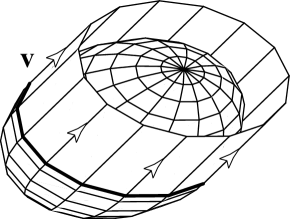
Figure 4: The pole of a diametral plane is the direction of the tangent cylinder to the quadric along its intersection.

We choose a basis of vectors $\{\vec{U},\vec{V},\vec{W}\}$, where

$$\vec{U}=\overrightarrow{TU},\quad\vec{V}=\overrightarrow{TV},\quad\vec{W}=\overrightarrow{TW},$$ (25)

if $U,V,W$ are proper points. If one of them is a point at infinity, we take it as vector of the basis. For instance, if $U$ is a point at infinity, we take $\vec{U}=U$.

The case of an improper point $T$ can be handled similarly. We use in this case a basis $\{\vec{U},\vec{V},\vec{T}\}$ with $\vec{U}=\overrightarrow{WU}$, $\vec{V}=\overrightarrow{WV}$, $\vec{T}=T$, if $W$ is a proper point. Otherwise, we choose $U$ or $V$ as origin and use $W$ as one of the vectors of the basis.

For a direction

$$\vec{v}=\alpha\vec{U}+\beta\vec{V}+\gamma\vec{W},$$ (26)

the polar plane is a diametral plane with linear form given by

$$\mathcal{Q}\vec{v}\!\!\!\!\! = \!\!\!\!\!\left(\frac{\gamma}{\Omega_{W}}-\frac{\alpha}{\Omega_{U}}-\frac{\beta}{\Omega_{V}}\right)\frac{p}{\Omega_{W}}+\left(\frac{\beta}{\Omega_{V}}-\frac{\alpha}{\Omega_{U}}-\frac{\gamma}{\Omega_{W}}\right)\frac{q}{\Omega_{V}}$$ (27)

$$+ \!\!\!\!\!\!\left(\frac{\alpha}{\Omega_{U}}-\frac{\beta}{\Omega_{V}}-\frac{\gamma}{\Omega_{W}}\right)\!\frac{r}{\Omega_{U}}-\lambda(\epsilon_{U}\alpha+\epsilon_{V}\beta+\epsilon_{W}\gamma)t.\quad$$

Before going on, we need information about the normal of a plane given by a linear form:

Lemma 1

A plane $l$ with linear form $ap+bq+cr+dt$, where $p,q,r,t$ are linear forms satisfying

$$p(W)=q(V)=r(U)=t(T)=1,$$

contains the vectors

$$\vec{v}_{1}=(b-\epsilon_{V}d)\vec{U}+(\epsilon_{U}d-c)\vec{V},$$

$$\vec{v}_{2}=(a-\epsilon_{W}d)\vec{V}+(\epsilon_{V}d-b)\vec{W},$$

$$\vec{v}_{3}=(\epsilon_{W}d-a)\vec{U}+(c-\epsilon_{U}d)\vec{W},$$

and hence its normal vector is given by

$$\vec{n}=(a-\epsilon_{W}d)\vec{U}\times\vec{V}+(c-\epsilon_{U}d)\vec{V}\times\vec{W}+(b-\epsilon_{V}d)\vec{W}\times\vec{U}.$$

The proof is simple, since a vector $\vec{v}=\alpha\vec{U}+\beta\vec{V}+\gamma\vec{W}$ belongs to the plane if and only if

$$0=l(\vec{v})=(c-\epsilon_{U}d)\alpha+(b-\epsilon_{V}d)\beta+(a-\epsilon_{W}d)\gamma.$$

A diametral plane is called a principal plane or a plane of symmetry if it is orthogonal to its pole $\vec{v}$. The principal axis of the quadric are the lines which are intersections of two principal planes. That is, the poles of the principal planes are the directions of the axes.

Since for this definition we need to include a scalar product, it is necessary to provide another symmetric bilinear form $G$, such that $\vec{v}\cdot\vec{w}=G(\vec{v},\vec{w})$, denoting by a dot the scalar product.

The matrix of such form is usually called Gram matrix and it is

$$G=\left(\begin{array}[]{ccc}g_{UU}&g_{UV}&g_{UW}\\ g_{VU}&g_{VV}&g_{VW}\\ g_{WU}&g_{WV}&g_{WW}\end{array}\right)\textrm{ where }g_{AB}:=\vec{A}\cdot\vec{B},$$ (31)

in the basis $\{\vec{U},\vec{V},\vec{W}\}$.

In order to derive conditions for principal planes, we have to impose that the pole $\vec{v}$ be orthogonal to a basis of vectors of the diametral plane, which can be two of the ones which have been calculated in Lemma 1,

$$0 = \vec{v}_{1}\cdot\vec{v}=(b-\epsilon_{V}d)(g_{UU}\alpha+g_{UV}\beta+g_{UW}\gamma)$$

$$+ (\epsilon_{U}d-c)(g_{VU}\alpha+g_{VV}\beta+g_{VW}\gamma),$$

$$0 = \vec{v}_{2}\cdot\vec{v}=(a-\epsilon_{W}d)(g_{VU}\alpha+g_{VV}\beta+g_{VW}\gamma)$$

$$+ (\epsilon_{V}d-b)(g_{WU}\alpha+g_{WV}\beta+g_{WW}\gamma),$$

and these equations can be easily solved up to a proportionality factor $\mu$,

$$a-\epsilon_{W}d = \mu(g_{WU}\alpha+g_{WV}\beta+g_{WW}\gamma),$$

$$b-\epsilon_{V}d = \mu(g_{VU}\alpha+g_{VV}\beta+g_{VW}\gamma),$$

$$c-\epsilon_{U}d = \mu(g_{UU}\alpha+g_{UV}\beta+g_{UW}\gamma),$$ (32)

where

$$a = \left(\frac{\gamma}{\Omega_{W}}-\frac{\alpha}{\Omega_{U}}-\frac{\beta}{\Omega_{V}}\right)\frac{1}{\Omega_{W}},$$

$$b = \left(\frac{\beta}{\Omega_{V}}-\frac{\alpha}{\Omega_{U}}-\frac{\gamma}{\Omega_{W}}\right)\frac{1}{\Omega_{V}},$$

$$c = \left(\frac{\alpha}{\Omega_{U}}-\frac{\beta}{\Omega_{V}}-\frac{\gamma}{\Omega_{W}}\right)\frac{1}{\Omega_{U}},$$

$$d = -\lambda(\epsilon_{U}\alpha+\epsilon_{V}\beta+\epsilon_{W}\gamma).$$ (33)

In the case of improper $T$ and, for instance, proper $W$, the equations for the coordinates of $\vec{v}=\alpha\vec{U}+\beta\vec{V}+\delta\vec{T}$ are

$$b-\epsilon_{V}a = \mu(g_{VU}\alpha+g_{VV}\beta+g_{VT}\delta),$$

$$c-\epsilon_{U}a = \mu(g_{UU}\alpha+g_{UV}\beta+g_{UT}\delta),$$

$$d = \mu(g_{TU}\alpha+g_{TV}\beta+g_{TT}\delta),$$ (34)

where

$$a = \left(-\frac{\epsilon_{U}\alpha+\epsilon_{V}\beta}{\Omega_{W}}-\frac{\alpha}{\Omega_{U}}-\frac{\beta}{\Omega_{V}}\right)\frac{1}{\Omega_{W}},$$

$$b = \left(\frac{\beta}{\Omega_{V}}-\frac{\alpha}{\Omega_{U}}+\frac{\epsilon_{U}\alpha+\epsilon_{V}\beta}{\Omega_{W}}\right)\frac{1}{\Omega_{V}},$$

$$c = \left(\frac{\alpha}{\Omega_{U}}-\frac{\beta}{\Omega_{V}}+\frac{\epsilon_{U}\alpha+\epsilon_{V}\beta}{\Omega_{W}}\right)\frac{1}{\Omega_{U}},$$

$$d = \lambda\delta.$$ (35)

These conditions can be seen as arising from an alternative definition of principal axes as lines with direction given by eigenvectors of the bilinear form of the conic at infinity. The values of the coefficient $\mu$ are the corresponding eigenvalues, which are obtained by imposing that the system (8) has non-trivial solutions for $\alpha,\beta,\gamma$. Hence $\mu$ has to satisfy a cubic equation and there are in general three principal planes and axes, except for quadrics of revolution and spheres:

Corollary 3

A rational triangular quadratic patch with control net $\{c_{002},c_{011},c_{020},c_{101},c_{110},c_{200}\}$ and weights $\{\omega_{002},\omega_{011},\omega_{020},\omega_{101},\omega_{110},\omega_{200}\}$, such that the three boundary conics meet at a point $S$, which is written as in (3), has diametral planes with linear forms given by (27) with a pole $\vec{v}=\alpha\vec{U}+\beta\vec{V}+\gamma\vec{W}$, or $\vec{v}=\alpha\vec{U}+\beta\vec{V}+\gamma\vec{T}$, if $T$ is a point at infinity, in a vector basis (25), defined with points (3) and (10).

The poles of principal planes are the directions of principal axes and, if $T$ is a proper point, they satisfy the linear system (8) for values of $\mu$ for which the determinant

$$\scriptsize{\left|\begin{array}[]{ccc}\lambda_{WU}-\frac{1}{\Omega_{W}\Omega_{U}}-\mu g_{WU}&\lambda_{WV}-\frac{1}{\Omega_{W}\Omega_{V}}-\mu g_{WV}&\lambda_{W}+\frac{1}{\Omega_{W}^{2}}-\mu g_{WW}\\[5.69054pt] \lambda_{VU}-\frac{1}{\Omega_{V}\Omega_{U}}-\mu g_{VU}&\lambda_{V}+\frac{1}{\Omega_{V}^{2}}-\mu g_{VV}&\lambda_{VW}-\frac{1}{\Omega_{V}\Omega_{W}}-\mu g_{VW}\\[5.69054pt] \lambda_{U}+\frac{1}{\Omega_{U}^{2}}-\mu g_{UU}&\lambda_{UV}-\frac{1}{\Omega_{U}\Omega_{V}}-\mu g_{UV}&\lambda_{UW}-\frac{1}{\Omega_{U}\Omega_{W}}-\mu g_{UW}\end{array}\right|}$$

vanishes, with $\lambda_{AB}:=\epsilon_{A}\epsilon_{B}\lambda$ and coefficients given by (3) and (31).

If $T$ is a point at infinity, the coordinates of the pole satisfy the linear system (8) for values of $\mu$ for which the determinant

$$\left|\begin{array}[]{ccc}A_{UU}-\mu g_{UU}&A_{UV}-\mu g_{UV}&-\mu g_{UT}\\ A_{UV}-\mu g_{VU}&A_{VV}-\mu g_{VV}&-\mu g_{VT}\\ -\mu g_{TU}&-\mu g_{TV}&\lambda-\mu g_{TT}\end{array}\right|$$

vanishes, with

$$A_{UU}:=\left(\frac{\epsilon_{U}}{\Omega_{W}}+\frac{1}{\Omega_{U}}\right)^{2},\quad A_{VV}:=\left(\frac{\epsilon_{V}}{\Omega_{W}}+\frac{1}{\Omega_{V}}\right)^{2},$$

$$A_{UV}:=\frac{\epsilon_{U}\epsilon_{V}}{\Omega_{W}^{2}}+\frac{\epsilon_{V}}{\Omega_{W}\Omega_{U}}+\frac{\epsilon_{U}}{\Omega_{W}\Omega_{V}}-\frac{1}{\Omega_{U}\Omega_{V}}.$$

In general there are three different values for $\mu$. If there is a double non-null solution, the quadric is a surface of revolution. If there is a triple solution, the surface is a sphere.

The discriminant of a cubic equation $a_{3}\mu^{3}+a_{2}\mu^{2}+a_{1}\mu+a_{0}=0$,

$$\Delta=-27a_{3}^{2}a_{0}^{2}+18a_{0}a_{1}a_{2}a_{3}-4a_{3}a_{1}^{3}-4a_{2}^{3}a_{0}+a_{2}^{2}a_{1}^{2},$$

provides a simple way of checking whether a quadric is a surface of revolution: A vanishing discriminant $\Delta$ is equivalent to having a double root.

Besides, a vanishing second derivative of the equation, $3a_{3}\mu+2a_{2}=0$, implies a triple root and hence the quadric would be a sphere.

It is easily checked that the eigenvalue $\mu=0$ just appears for $\lambda^{-1}=\tilde{\Omega}_{U}\tilde{\Omega}_{V}+\tilde{\Omega}_{V}\tilde{\Omega}_{W}+\tilde{\Omega}_{W}\tilde{\Omega}_{U}$ in the case of proper $T$. That is, for paraboloids. For these surfaces the plane at infinity is a principal plane: The plane at infinity is diametral, as it comprises the center, and it is principal, since it fulfills (8). Besides, it is the polar plane of the center, since it is tangent to the paraboloid at the center.

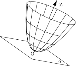
Figure 5: The vertex $O$ of a paraboloid is the pole of a tangent plane with the center $Z$ as normal.

In the case of improper $T$, the eigenvalue $\mu=0$ appears only if $\lambda=0$. Hence, cylinders have a null eigenvalue, corresponding to a pole $T$, the direction of the axis, which has no polar plane. For parabolic cylinders there is another null eigenvalue, since the plane at infinity is an improper principal plane.

There are then just two proper principal planes for paraboloids, except for paraboloids of revolution. The intersection of these principal planes is the only proper axis of the paraboloid, a line with direction given by the center of the paraboloid. The axis meets the paraboloid at the center and at a single proper point named vertex.

We may calculate the vertex solving a quadratic equation, but there is a simpler way, taking into account that the tangent plane $o$ at the vertex $O$ is orthogonal to the center $Z$ (see Fig. 5). We can use this property to compute the vertex:

A plane with linear form $ap+bq+cr+dt$ is orthogonal to a vector (26) if their coordinates fulfill (8). Hence reading the coordinates of $Z$ from (16) with, for instance, $\mu=1$,

$$\alpha=\Omega_{U}(\tilde{\Omega}_{V}+\tilde{\Omega}_{W}),\quad\beta=\Omega_{V}(\tilde{\Omega}_{W}+\tilde{\Omega}_{U}),$$

$$\gamma=\Omega_{W}(\tilde{\Omega}_{U}+\tilde{\Omega}_{V}),$$

we get the differences $A=a-\epsilon_{W}d$, $B=b-\epsilon_{V}d$, $C=c-\epsilon_{U}d$ for the planes which are orthogonal to the center. That is, we have the linear form for the tangent plane at the vertex of the paraboloid, except for the coefficient $d$. Since tangent planes are solutions of the implicit equation of the quadric in tangential form (13),

$$0\!\!\! = \!\!\!\Omega_{U}\Omega_{V}(C+\epsilon_{U}d)(B+\epsilon_{V}d)$$

$$+ \!\!\!\Omega_{V}\Omega_{W}(B+\epsilon_{V}d)(A+\epsilon_{W}d)$$

$$+ \!\!\!\Omega_{W}\Omega_{U}(A+\epsilon_{W}d)(C+\epsilon_{U}d)$$

$$- \!\!\!\frac{1}{\tilde{\Omega}_{U}\tilde{\Omega}_{V}+\tilde{\Omega}_{V}\tilde{\Omega}_{W}+\tilde{\Omega}_{W}\tilde{\Omega}_{U}}$$

$$= \!\!\!\Omega_{U}\Omega_{V}BC+\Omega_{V}\Omega_{W}AB+\Omega_{W}\Omega_{U}AD$$

$$+ \!\!\!\big{(}\Omega_{U}\Omega_{V}(\epsilon_{U}B+\epsilon_{V}C)+\Omega_{V}\Omega_{W}(\epsilon_{V}A+\epsilon_{W}B)$$

$$+ \!\!\!\Omega_{W}\Omega_{U}(\epsilon_{U}A+\epsilon_{W}C)\big{)}d,$$

the coefficients of the plane are readily obtained

$$d\!\!\!\! = \!\!\!\!-\frac{\Omega_{U}\Omega_{V}BC+\Omega_{V}\Omega_{W}AB+\Omega_{W}\Omega_{U}AC}{\scriptstyle{\Omega_{U}\Omega_{V}(\epsilon_{U}B+\epsilon_{V}C)+\Omega_{V}\Omega_{W}(\epsilon_{V}A+\epsilon_{W}B)+\Omega_{W}\Omega_{U}(\epsilon_{U}A+\epsilon_{U}C)}},$$

$$a\!\!\!\! = \!\!\!\!\epsilon_{W}d+g_{WU}\Omega_{U}(\tilde{\Omega}_{V}+\tilde{\Omega}_{W})+g_{WV}\Omega_{V}(\tilde{\Omega}_{W}+\tilde{\Omega}_{U})$$

$$+ \!\!\!\!g_{WW}\Omega_{W}(\tilde{\Omega}_{U}+\tilde{\Omega}_{V}),$$

$$b\!\!\!\! = \!\!\!\!\epsilon_{V}d+g_{VU}\Omega_{U}(\tilde{\Omega}_{V}+\tilde{\Omega}_{W})+g_{VV}\Omega_{V}(\tilde{\Omega}_{W}+\tilde{\Omega}_{U})$$

$$+ \!\!\!\!g_{VW}\Omega_{W}(\tilde{\Omega}_{U}+\tilde{\Omega}_{V}),$$

$$c\!\!\!\! = \!\!\!\!\epsilon_{U}d+g_{UU}\Omega_{U}(\tilde{\Omega}_{V}+\tilde{\Omega}_{W})+g_{UV}\Omega_{V}(\tilde{\Omega}_{W}+\tilde{\Omega}_{U})$$ (36)

$$+ \!\!\!\!g_{UW}\Omega_{W}(\tilde{\Omega}_{U}+\tilde{\Omega}_{V}),$$

where $a,b,c,d$ are given by (8).

The vertex $O$ is just the pole of the plane $o=ap+bq+cr+dt$:

Corollary 4

A rational triangular quadratic patch for a paraboloid with control net $\{c_{002},c_{011},c_{020},c_{101},c_{110},c_{200}\}$ and weights $\{\omega_{002},\omega_{011},\omega_{020},\omega_{101},\omega_{110},\omega_{200}\}$, such that the three boundary conics meet at a point $S$, which is written as in (3), has a vertex given by

$$O\!\!\!\!\! = \!\!\!\!\!\frac{(b\Omega_{V}+a\Omega_{W})\Omega_{U}U+(c\Omega_{U}+a\Omega_{W})\Omega_{V}V}{\scriptstyle{\Omega_{U}\Omega_{V}(b+c-2\epsilon_{U}\epsilon_{V}d)+\Omega_{V}\Omega_{W}(a+b-2\epsilon_{V}\epsilon_{W}d)+\Omega_{W}\Omega_{U}(a+c-2\epsilon_{W}\epsilon_{U}d)}}$$

$$+ \!\!\!\!\!\frac{(c\Omega_{U}+b\Omega_{V})\Omega_{W}W-2d(\tilde{\Omega}_{U}\tilde{\Omega}_{V}+\tilde{\Omega}_{V}\tilde{\Omega}_{W}+\tilde{\Omega}_{W}\tilde{\Omega}_{U})T}{\scriptstyle{\Omega_{U}\Omega_{V}(b+c-2\epsilon_{U}\epsilon_{V}d)+\Omega_{V}\Omega_{W}(a+b-2\epsilon_{V}\epsilon_{W}d)+\Omega_{W}\Omega_{U}(a+c-2\epsilon_{W}\epsilon_{U}d)}},$$

where $A=a-\epsilon_{W}d$, $B=b-\epsilon_{V}d$, $C=c-\epsilon_{U}d$ and (8). The coefficients are given in (3) and (19) and the points $U,V,W,T$ are defined in (3) and (10).

Finally, the axis of a cylinder is easily determined, since it has the direction of $T$ and contains the center of every conic section. For instance, we can use the center of the conic at $t$, which according to (17) is given by

$$Z_{t}=\frac{\epsilon_{W}\Omega_{W}\omega_{w}\omega_{002}P+\epsilon_{V}\Omega_{V}\omega_{v}\omega_{020}Q+\epsilon_{U}\Omega_{U}\omega_{u}\omega_{200}R}{\Omega_{Z}}.$$

9 Examples

Now we apply our results to several quadric patches:

Example 1

Net: $\left[\begin{array}[]{c}(0,0,0)\hskip 5.69046pt(1,0,1)\hskip 5.69046pt(2,0,0)\\ (-2,2,3)\hskip 5.69046pt(1,1,1)\\ (0,\frac{4}{3},\frac{2}{3})\end{array}\right]$ and weights: $\left[\begin{array}[]{c}1\hskip 5.69046pt\frac{1}{2}\hskip 5.69046pt1\\ \frac{1}{3}\hskip 2.84544pt\frac{2}{3}\\ 1\end{array}\right]$ (Fig. 6):

Figure 6: Ellipsoid

The normalised linear forms for the tangent planes are

$$p=\frac{10x+25y-10z}{32},\ q=\frac{2-x-z}{8},\ r=\frac{12-3x-9y}{16},$$

and meet at a point $(-8/7,12/7,22/7)$.

The three boundary conics meet at a point,

$$S = (1,0,-1)=c_{002}-c_{011}+c_{020}$$

$$= \frac{c_{002}-2c_{101}/3+c_{200}}{4/3}=\frac{c_{200}-4c_{110}/3+c_{020}}{2/3},$$

and hence $\omega_{u}=1$, $\omega_{v}=4/3$, $\omega_{w}=2/3$.

The normalised linear form for the plane through the corners of the net is

$$t=\frac{-7y+14z}{32}.$$

The quadric is oval, since the coefficient $\lambda=207/49$ for this quadric patch is positive.

It is not a paraboloid, since the center is the proper point $(1/2,2/5,-1/30)$. Since the boundary curves and the conic on $t$ are ellipses, the quadric is an ellipsoid. One arrives to the same conclusion checking that $\det\mathcal{Z}=480/49$ is positive.

The bilinear form that we get for this surface is

$$\mathcal{Q}=\frac{18x^{2}+45xy+81y^{2}-81yz+54z^{2}-36x-90y+36z}{64},$$

and the implicit equation, in cartesian coordinates is

$$0=18x^{2}+45xy+81y^{2}-81yz+54z^{2}-36x-90y+36z.$$

The three eigenvalues calculated according to Corollary 3 are different, $\mu=1.78,0.90,0.52$, and so this ellipsoid is not a surface of revolution.

The three principal planes are

$$0.61p+0.37q-1.32r-2.04t,$$

$$-0.90p+15.05q-4.49r+5.04t,$$

$$-10.46p+17.24q-0.57r-19.12t,$$

with respective implicit equations in cartesian coordinates

$$0.39x+1.67y-1.13z-0.90=0,$$

$$-1.32x+0.72y+0.60z+0.39=0,$$

$$-5.32x-3.67y-7.25z+3.88=0,$$

and obviously meet at the center.

Example 2

Net: $\left[\begin{array}[]{c}(0,0,0)\hskip 5.69046pt(1,0,1)\hskip 5.69046pt(2,0,0)\\ (-1,1,2)\hskip 5.69046pt(1,\frac{1}{2},1)\\ (0,2,0)\end{array}\right]$ and weights: $\left[\begin{array}[]{c}1\hskip 5.69046pt2\hskip 5.69046pt3\\ 1\hskip 5.69046pt2\\ 1\end{array}\right]$ (Fig. 7):

Figure 7: Two-sheeted hyperboloid

The normalised linear forms for the tangent planes are

$$p=\frac{x+3y-z}{4},\ q=\frac{x+z-2}{4},\ r=\frac{12-4x-6y-5z}{8},$$

and meet at a point $(2/5,2/5,8/5)$.

The three boundary conics meet at a point at infinity,

$$S = (2,0,-4)=c_{002}-4c_{011}+3c_{020}$$

$$= c_{002}-2c_{101}+c_{200}=c_{200}-4c_{110}+3c_{020},$$

and hence $\omega_{u}=\omega_{v}=\omega_{w}=1$.

The normalised linear form for the plane through the corners of the net is

$$t=\frac{5z}{8}.$$

The quadric is oval, since the coefficient $\lambda=3/25$ for this quadric patch is positive.

It is not a paraboloid, since the center is the proper point $(7/4,-1/2,5/2)$. As the boundary curves are not ellipses, but two hyperbolas and one parabola, the quadric is not an ellipsoid, but a two-sheeted hyperboloid. Accordingly, $\det\mathcal{Z}=-16/25$ is negative.

The bilinear form that we get for this surface is

$$\mathcal{Q}=\frac{4x^{2}+12xy+12y^{2}+6yz-z^{2}-8x-24y+8z}{48},$$

and the implicit equation, in cartesian coordinates is

$$0=4x^{2}+12xy+12y^{2}+6yz-z^{2}-8x-24y+8z.$$

The eigenvalues for the normal directions of the principal planes are different, $\mu=0.33,-0.44,0.30$, and hence the hyperboloid is not a surface of revolution.

The principal planes are

$$1.58p+0.45q-0.91r+0.08t,$$

$$0.36p+0.05q+0.30r+0.22t,$$

$$0.79p+4.65q+1.21r-0.96t,$$

and have the respective equations in cartesian coordinates

$$0.97x+1.87y+0.34z-1.60=0,$$

$$-0.05x+0.05y-0.13z+0.43=0,$$

$$0.75x-0.32y-0.39z-0.51=0,$$

and meet at the center as expected.

Example 3

Net: $\left[\begin{array}[]{c}(0,0,0)\hskip 5.69046pt(1,0,0)\hskip 5.69046pt(2,0,2)\\ (0,\frac{1}{2},0)\hskip 5.69046pt(1,\frac{1}{2},0)\\ (0,1,-\frac{1}{2})\end{array}\right]$ and weights: $\left[\begin{array}[]{c}1\hskip 5.69046pt1\hskip 5.69046pt1\\ 1\hskip 5.69046pt1\\ 1\end{array}\right]$ (Fig. 8)

Figure 8: Hyperbolic paraboloid

The normalised linear forms for the tangent planes are

$$p=-z,\ q=\frac{4-4x+2z}{3},\ r=\frac{-1+2y+2z}{3},$$

and meet at a point $(1,1/2,0)$.

The three boundary conics meet at a point at infinity,

$$S = (0,0,2)=c_{002}-2c_{011}+c_{020}$$

$$= \frac{c_{002}-2c_{101}+c_{200}}{-1/4}=\frac{c_{200}-2c_{110}+c_{020}}{3/4},$$

and hence $\omega_{u}=1$, $\omega_{v}=-1/4$, $\omega_{w}=3/4$.

The normalised linear form for the plane through the corners of the net is

$$t=\frac{4x-2y-4z}{3}.$$

The quadric is ruled, since the coefficient $\lambda=-1$ for this quadric patch is negative.

It is a hyperbolic paraboloid, since the center is a point at infinity $(0,0,-3/64)$, which is also the direction of the axis.

The bilinear form that we get for this surface is

$$\mathcal{Q}=\frac{8z-4x^{2}+4y^{2}}{3},$$

and the implicit equation, in cartesian coordinates is

$$0=2z-x^{2}+y^{2}.$$

The eigenvalues calculated according to Corollary 3 are different, $\mu=0,4/3,-4/3$, and one of them is null, as it is expected for a hyperbolic paraboloid.

The three principal planes are

$$q+r+t,$$

$$2p+q+4r+t,$$

$$-\frac{3}{2}p+\frac{3}{4}q+3r+3t.$$

The first principal plane is the plane at infinity and the other ones have $y=0$, $x=0$ as implicit equations in cartesian coordinates. They all meet at the center.

The vertex is the point $(0,0,0)$, as it is clear from the form of the implicit equation.

Example 4

Net: $\left[\begin{array}[]{c}(0,-1,0)\hskip 2.84544pt(2,0,0)\hskip 2.84544pt(0,1,0)\\ (1,-\frac{1}{2},\frac{1}{2})\hskip 2.84544pt(1,\frac{1}{2},1)\\ (1,0,1)\end{array}\right]$ and weights: $\left[\begin{array}[]{c}1\hskip 5.69046pt1\hskip 5.69046pt1\\ 1\hskip 5.69046pt1\\ 1\end{array}\right]$ (Fig. 9):

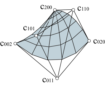
Figure 9: Parabolic cylinder

The normalised linear forms for the tangent planes are

$$p=1-\frac{x}{2}+y,\ q=1-\frac{x}{2}-y,\ r=x-1,$$

and meet at a point at infinity $(0,0,1)$.

The three boundary conics are parabolas and do not meet at any point. Hence the patch does not belong to a non-degenerate quadric. If it is a degenerate quadric, it is then a parabolic cylinder with direction $(0,0,1)$. It is easy to check, for instance, that their respective centers are aligned and hence it is a degenerate quadric.

The normalised linear form for the plane through the corners of the net is

$$t=-x+z.$$

Using (6) we find a set of weights $\Omega_{U}=-1/2$, $\Omega_{V}=1=\Omega_{W}$ and hence the bilinear form that we get for this surface is

$$\mathcal{Q}=4(x+y^{2}-1),$$

and the implicit equation, in cartesian coordinates is

$$x=1-y^{2}.$$

The eigenvalues for the poles of the principal planes are $\mu=0,0,4$, as it is expected for a parabolic cylinder.

The principal planes are

$$p+q+r,\qquad p-q.$$

The first one is the plane at infinity and the second one is the only proper principal plane of a parabolic cylinder, with equation in cartesian coordinates given by $y=0$.

Example 5

Net:$\left[\begin{array}[]{c}(2,0,2)\hskip 1.42262pt(\frac{4}{3},\frac{4\sqrt{3}}{9},\frac{4}{3})\hskip 1.42262pt(\frac{1}{2},\frac{\sqrt{3}}{2},1)\\[2.84526pt] (\frac{4}{3},-\frac{4\sqrt{3}}{9},\frac{4}{3})\hskip 1.42262pt(2,0,1)\\[2.84526pt] (\frac{1}{2},-\frac{\sqrt{3}}{2},1)\end{array}\right]$ and weights: $\left[\begin{array}[]{c}\frac{3}{8}\hskip 5.69046pt\frac{9}{16}\hskip 5.69046pt1\\ \frac{9}{16}\hskip 5.69046pt\frac{1}{2}\\ 1\end{array}\right]$ (Fig. 10):

The normalised linear forms for the tangent planes are

$$p=\frac{z-x}{2},\ q=\frac{-x-\sqrt{3}y+2z}{4},\ r=\frac{-x+\sqrt{3}y+2z}{4},$$

and meet at a point $(0,0,0)$.

The three boundary conics meet at a point

$$S = (-1,0,1)=\frac{3c_{002}/8-9c_{011}/8+c_{020}}{1/4}$$

$$= \frac{3c_{002}/8-9c_{101}/8+c_{200}}{1/4}=c_{200}-c_{110}+c_{020},$$

and hence $\omega_{u}=1/4=\omega_{v}$, $\omega_{w}=1$.

The normalised linear form for the plane through the corners of the net is

$$t=\frac{2+2x-3z}{2}.$$

The quadric is degenerate, since the coefficient for this quadric patch is $\lambda=0$. It is a cone, since the intersection of the tangent planes is a proper point, which is the vertex $(0,0,0)$.

The bilinear form that we get for this surface is

$$\mathcal{Q}=\frac{16}{3}(x^{2}+y^{2}-z^{2}),$$

and the implicit equation, in cartesian coordinates is

$$0=x^{2}+y^{2}-z^{2}.$$

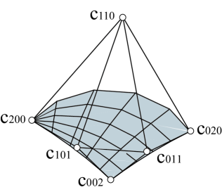
Figure 10: Cone

The eigenvalues for the poles of the principal planes are $\mu=-16/3,16/3,16/3$, and so the surface is a cone of revolution.

The principal planes are

$$p-q-r,$$

$$3\gamma p+(1-2\gamma)q-(1+\gamma)r,$$

for every value of $\gamma$ and their respective equations in cartesian coordinates are

$$z=0,$$

$$3\gamma x+(2-\gamma)\sqrt{3}y=0.$$

10 Tensor product quadric patches

Tensor product patches are the most common way to model surfaces in CAD. In particular, in some cases quadrics can be parametrised by biquadratic rational Bézier patches,

$$c(u,v)=\frac{\displaystyle\sum_{i=0}^{2}\sum_{j=0}^{2}\omega_{ij}c_{ij}B^{2}_{i}(u)B^{2}_{j}(v)}{\displaystyle\sum_{i=0}^{2}\sum_{j=0}^{2}\omega_{ij}B^{2}_{i}(u)B^{2}_{j}(v)},\quad u,v\in[0,1],$$

for a control net $\{c_{00},c_{01},c_{02},c_{10},c_{11},c_{12},c_{20},c_{21},c_{22}\}$ and their respective weights.

The patch is bounded by four conic arcs with control polygons $\{c_{00},c_{01},c_{02}\}$, $\{c_{20},c_{21},c_{22}\}$, $\{c_{00},c_{10},c_{20}\}$ and $\{c_{02},c_{12},c_{22}\}$, meeting two by two at the four corner vertices $c_{00}$, $c_{02}$, $c_{20}$, $c_{22}$.

Not every rational biquadratic patch is a quadric patch [21, 22], but we can apply our knowledge about quadric triangular patches to them.

For instance, we can take $P=c_{00}$, $Q=c_{02}$, $R=c_{20}$ and define a triangular patch with these three corners, as we know that the tangent planes are defined by the neighbouring vertices: $p$ contains $c_{00},c_{01},c_{10}$, $q$ contains $c_{02},c_{01},c_{12}$ and $r$ contains $c_{20}$, $c_{10}$, $c_{21}$ (see Fig. 11).

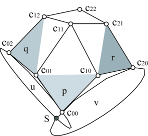
Figure 11: Planes on a biquadratic tensor product patch

We already know the conic at $u$, defined by the control points $\{c_{00},c_{01},c_{02}\}$ and their weights, and the conic at $v$, defined by $\{c_{00},c_{10},c_{20}\}$ and their weights. For the conic at $w$ we have the control points $c_{02}$ and $c_{20}$ and their weights, but we lack the intermediate control point $c_{110}$ and the weight $\omega_{110}$.

In order to have a triangular quadric patch, we can use the other point $S$ where the conics at $u$ and $v$ meet, besides $P$. We may reparametrise both conics as we did in (3) so that their weights satisfy

$$S=\frac{\omega_{00}c_{00}-2\omega_{01}c_{01}+\omega_{02}c_{02}}{\omega_{u}}=\frac{\omega_{00}c_{00}-2\omega_{10}c_{10}+\omega_{20}c_{20}}{\omega_{v}},$$

where denominators, if $S$ is a proper point, are

$$\omega_{u}=\omega_{00}-2\omega_{01}+\omega_{02},\quad\omega_{v}=\omega_{00}-2\omega_{10}+\omega_{20}.$$

Now we can define the plane $w$ as the one containing $S,c_{02},c_{20}$ and complete Fig. 2 by computing the intersection points $U,V,W$ on plane $t$.

The barycentric combinations for $U,V,W$ provide us the value of $\omega_{w}$ and hence of $\omega_{110}$ and $c_{110}$.

If the biquadratic patch is in fact part of a quadric surface, Theorem 1 provides its bilinear forms and we can calculate its geometric elements. We see it with an example:

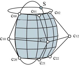
Figure 12: Spherical rational tensor product patch

Example 6

Net:$\left[\begin{array}[]{ccc}(a,0,a)&(a,a,a)&(0,a,a)\\ (2a,0,0)&(2a,2a,0)&(0,2a,0)\\ (a,0,-a)&(a,a,-a)&(0,a,-a)\end{array}\right]$ with $a=1/\sqrt{2}$ and weights: $\left[\begin{array}[]{ccc}1&1&2\\ 1/2&1/2&1\\ 1/2&1/2&1\end{array}\right]$ (Fig. 12):

We use a triangular patch through $P=c_{00}$, $Q=c_{02}$, $R=c_{20}$ with the following control net and weights

$$\left[\begin{array}[]{c}(a,0,a)\hskip 2.84544pt(a,a,a)\hskip 2.84544pt(0,a,a)\\ (2a,0,0)\hskip 2.84544ptc_{110}\\ (a,0,-a)\end{array}\right],\quad\left[\begin{array}[]{c}1\hskip 14.22636pt1\hskip 14.22636pt2\\ 1/2\hskip 2.84544pt\omega_{110}\\ 1/2\end{array}\right],$$

and notice that the conic at $u$ and the conic at $v$ meet at the point $S=(-\sqrt{2}/2,0,\sqrt{2}/2)$ and

$$S=c_{00}-2c_{01}+2c_{02}=\frac{c_{00}-c_{10}+c_{20}/2}{1/2}.$$

There is no need to perform Möbius transformations, since the weights already satisfy

$$\omega_{u}=\omega_{00}-2\omega_{01}+\omega_{02}=1,\quad\omega_{v}=\omega_{00}-2\omega_{10}+\omega_{20}=\frac{1}{2},$$

but the other denominator is not determined,

$$\omega_{w}=\omega_{20}-2\omega_{110}+\omega_{02}=\frac{5}{2}-2\omega_{110}.$$

The control points and $S$ define the planes $p,q,r,t$ and their intersections,

$$U=\left(\frac{\sqrt{2}}{4},\frac{\sqrt{2}}{4},\frac{3\sqrt{2}}{4}\right),\quad V=\left(\sqrt{2},-\frac{\sqrt{2}}{2},0\right),$$

$$T=(1,\sqrt{2},\sqrt{2},0),$$

except for $W$, which is a point at infinity with direction $(1,-1,1)$.

This means that $\Omega_{W}=1$, but the normalisation term for $W$

$$-\omega_{002}\omega_{w}+\omega_{020}\omega_{v}+\omega_{200}\omega_{u}=2\omega_{110}-1$$

must vanish and hence $\omega_{110}=1/2$, $\omega_{w}=3/2$ and the representative for $W$ is the vector

$$W=-\omega_{00}\omega_{w}P+\omega_{02}\omega_{v}Q+\omega_{21}\omega_{u}=\frac{\sqrt{2}}{2}\left(-1,1,-1\right).$$

The coefficients

$$\Omega_{U}=2,\quad\Omega_{V}=1,\quad\Omega_{W}=1,\quad\lambda=2,$$

yield the expression for the bilinear form for the quadric,

$$\mathcal{Q}=p^{2}+q^{2}+\frac{r^{2}}{4}-2pq-pr-qr+2t^{2}.$$

The normalised forms for the planes are

$$p=-\frac{\sqrt{2}}{2}(x+z-\sqrt{2}),\quad q=\frac{\sqrt{2}}{3}(\sqrt{2}-y-z),$$

$$r=\frac{\sqrt{2}}{3}(\sqrt{2}-x+z),\quad t=\frac{\sqrt{2}}{3}\left(x+y-\frac{\sqrt{2}}{2}\right),$$

and so the implicit equation for the surface in cartesian coordinates is

$$x^{2}+y^{2}+z^{2}-1=0.$$

11 Conclusions

We have derived closed formulas in terms of control points and weights for several geometric elements of quadrics in rational Bézier form, both in triangular and tensor product representation. To our knowledge, these formulas have not been produced before. The main difference with other procedures for drawing geometric information from rational triangular patches [3] is the use of geometric entities such as tangent planes to the quadric and their intersections as ingredients for obtaining bilinear forms, and hence, implicit equations, for the surface. There are many ways of implicitising a parametric surface [23], but the use of linear forms with geometrical meaning instead of cartesian coordinates simplifies this problem for quadric patches. Besides, these geometric entities appear naturally in the formulas for geometric elements because they are already present in the expressions for the bilinear forms for the quadric. The use of projective algebraic geometry allows us to perform calculations in a synthetic fashion, instead of resorting to cartesian coordinates.

Additionally we classify affine quadrics using one coefficient involving the weights of the patch. This can be done without implicitising the quadric patch [10, 12], but the closed form for the implicit equations is what enables us to derive closed formulas for geometric elements.

The results are obtained initially for Bézier triangles, but are also extended to quadric patches in tensor product form.

References

Pottmann et al. [2007]
H. Pottmann, A. Asperl,
M. Hofer, A. Kilian.,
Architectural geometry, Bentley
Institute Press, Exton, 2007.
Sederberg and Anderson [1985]
T. Sederberg, D. Anderson,
Steiner Surface Patches, IEEE Computer
Graphics and Applications 5 (1985)
23–36.
Boehm and Hansford [1991]
W. Boehm, D. Hansford,
Bézier Patches on Quadrics, in:
G. Farin (Ed.), NURBS for Curves and
Surface Design, SIAM, 1–14,
1991.
Lodha and Warren [1990]
S. Lodha, J. Warren,
Bézier representation for quadric surface patches,
Computer-Aided Design
22 (9) (1990)
574 – 579.
Dietz et al. [1993]
R. Dietz, J. Hoschek,
B. Jüttler, An algebraic approach to
curves and surfaces on the sphere and on other quadrics,
Computer Aided Geometric Design
10 (3-4) (1993)
211 – 229.
Dietz et al. [1995]
R. Dietz, J. Hoschek,
B. Jüttler, Rational patches on quadric
surfaces, Computer-Aided Design
27 (1) (1995)
27 – 40.
Coffman et al. [1996]
A. Coffman, A. J. Schwartz,
C. Stanton, The algebra and geometry of
Steiner and other quadratically parametrizable surfaces,
Computer Aided Geometric Design
13 (3) (1996)
257 – 286.
Degen [1996]
W. Degen, The Types of Triangular Bézier
Surfaces, in: G. Mullineux (Ed.), The
Mathematics of Surfaces VI, Clarendon Press,
153–170, 1996.
Albrecht [1998a]
G. Albrecht, Determination and classification
of triangular quadric patches, Computer Aided Geometric
Design 15 (7)
(1998a) 675 – 697.
Albrecht [1998b]
G. Albrecht, Rational quadratic Bezier
triangles on quadrics, in: F.-E. Wolter,
N. Patrikalakis (Eds.), Computer
Graphics International, 1998. Proceedings, IEEE,
Los Alamitos, CA, 34–40,
1998b.
Albrecht [2011]
G. Albrecht, Geometric invariants of
parametric triangular quadric patches, International
Electronic Journal of Geometry 4 (2)
(2011) 63 – 84.
Sánchez-Reyes and Paluszny [2000]
J. Sánchez-Reyes, M. Paluszny,
Weighted radial displacement: A geometric look at Bézier
conics and quadrics, Computer Aided Geometric Design
17 (3) (2000)
267 – 289.
Albrecht [2004]
G. Albrecht, An Algorithm for Parametric
Quadric Patch Construction, Computing
72 (1-2) (2004)
1–12.
Albrecht et al. [2015]
G. Albrecht, M. Paluszny,
M. Lentini, An intuitive way for
constructing parametric quadric triangles, Computational
and Applied Mathematics (2015) 1–23.
Cantón et al. [2011]
A. Cantón, L. Fernández-Jambrina,
E. Rosado-María, Geometric
characteristics of conics in Bézier form,
Computer-Aided Design
43 (11) (2011)
1413 – 1421.
Albrecht [1999]
G. Albrecht, Rational Triangular Bézier
Surfaces - Theory and Applications, Habilitationschrift,
Fakultät für Mathematik, TU München, Shaker-Verlag,
Aachen, 1999.
Farin [2002]
G. Farin, Curves and surfaces for CAGD: a
practical guide, Morgan Kaufmann Publishers Inc.,
San Francisco, CA, USA, 5th edn., ISBN
1-55860-737-4, 2002.
Cantón et al. [2015]
A. Cantón, L. Fernández-Jambrina,
E. Rosado María, M. Váquez-Gallo,
Implicit Equations of Non-degenerate Rational Bézier
Quadric Triangles, in: J.-D. Boissonnat,
A. Cohen, O. Gibaru,
C. Gout, T. Lyche, M.-L.
Mazure, L. L. Schumaker (Eds.), Curves
and Surfaces, vol. 9213 of Lecture
Notes in Computer Science, Springer International
Publishing, ISBN 978-3-319-22803-7, 70–79,
2015.
Semple and Kneebone [1952]
J. G. Semple, G. T. Kneebone,
Algebraic projective geometry, Oxford
University Press, London, 1952.
Boehm [1993]
W. Boehm, Some remarks on quadrics,
Computer Aided Geometric Design
10 (3–4) (1993)
231 – 236.
Fink [1992]
U. Fink, Biquadratische
Bézier-Flächenstücke auf Quadriken, Master’s thesis,
Fakultät Mathematik der Universität Stuttgart,
Mathematisches Institut der Universität Stuttgart,
1992.
Sederberg et al. [1984]
T. Sederberg, D. Anderson,
R. Goldman, Implicit representation of
parametric curves and surfaces, Computer Vision, Graphics,
and Image Processing 28 (1)
(1984) 72 – 84.