Self-dual configurations in a generalized Abelian Chern-Simons-Higgs model with explicit breaking of the Lorentz covariance

Abstract

Abstract

We have studied the existence of self-dual solitonic solutions in a generalization of the Abelian Chern-Simons-Higgs model. Such a generalization introduces two different nonnegative functions, $\omega_{1}(|\phi|)$ and $\omega(|\phi|)$, which split the kinetic term of the Higgs field - $|D_{\mu}\phi|^{2}\rightarrow\omega_{1}(|\phi|)|D_{0}\phi|^{2}-\omega(|\phi|)|D_{k}\phi|^{2}$ - breaking explicitly the Lorentz covariance. We have shown that a clean implementation of the Bogomolnyi procedure only can be implemented whether $\omega(|\phi|)\propto\beta|\phi|^{2\beta-2}$ with $\beta\geq 1$. The self-dual or Bogomolnyi equations produce an infinity number of soliton solutions by choosing conveniently the generalizing function $\omega_{1}(|\phi|)$ which must be able to provide a finite magnetic field. Also, we have shown that by properly choosing the generalizing functions it is possible to reproduce the Bogomolnyi equations of the Abelian Maxwell-Higgs and Chern-Simons-Higgs models. Finally, some new self-dual $|\phi|^{6}$-vortex solutions have been analyzed both from theoretical and numerical point of view.

I Introduction

A time ago it was shown that (1+2)-dimensional matter field interacting with gauge fields whose dynamics is governed by a Chern-Simons term support soliton solutions Jk1 , Jk2 (for a review see Refs. hor1 , hor2 , hor3 , hor4 and hor5 ). These models have the particularity to become self-dual when the self-interactions are suitably chosen JW1 , JW2 , JP1 , JP2 . When self-duality occurs the model presents interesting mathematical and physical properties, such as the second order Euler-Lagrange equations can be solved by a set of first-order differential equations Bogo , Vega and, the model admits a supersymmetric extension LLW . The Chern-Simons gauge field dynamic remains the same when coupled with matter-fields either relativistic JW1 , JW2 or nonrelativistic JP1 , JP2 . In addition the nature of the soliton solutions can be topological and/or nontopological JLW .

The inclusion of non-linear terms to the kinetic part of the Lagrangian has interesting consequences, as for example, the existence of topological defects without a symmetry-breaking potential term sy . In the recent years, theories with nonstandard kinetic term, named $k$-field models, have received much attention. The $k$-field models are mainly in connection with effective cosmological models APDM1 , APDM2 , APDM3 , APDM4 , APDM5 , APDM6 , APDM7 , as well as the tachyon matter 12 and the ghost condensates 131 , 132 , 133 , 134 , 135 . The strong gravitational waves MV and dark matter APL , are also examples of non-canonical fields in cosmology. The investigations concerning to the topological structure of the $k$-field theories have shown that they support topological soliton solutions both in pure matter models as in gauged field models BAi1 , BAi2 , BAi3 ,BAi4 , BAi5 , BAi6 , BAi7 , BAi8 , SG1 ,SG2 , SG3 , SG4 , SG5 , SG6 , lucas1 ,lucas2 , lucas3 , lucas4 . These solitons have certain features which are not necessarily shared with those of the standard models B1 , B2 , B3 .

The aim of this manuscript is to study a Chern-Simons-Higgs model with a generalized dynamics which breaks Lorentz covariance, i.e,

$$|D_{\mu}\phi|^{2}\rightarrow\omega_{1}(|\phi|)|D_{0}\phi|^{2}-\omega(|\phi|)|D_{i}\phi|^{2}.$$ (1)

The nonstandard dynamics is introduced by the functions $\omega_{1}$ and $\omega$, depending on the Higgs field. During the implementation of Bogomolnyi trick is demonstrated that self-dual configurations exist if the function $\omega$ is proportional to $|\phi|^{2\beta-2}$ with $\beta\geq 1$. On the other hand, the function $\omega_{1}$ remains arbitrary but near the origin should behave as $|\phi|^{2\delta}$ with $\delta\geq-1$ in order to have a well behavior for the magnetic field. In particular we have chosen the functions $\omega_{1}$ and $\omega$, to be

$$\omega_{1}(|\phi|)=|\phi|^{2M},~{}\omega(|\phi|)=(N+1)|\phi|^{2N},$$ (2)

where $M\geq-1$ and $N\geq 0$. This way, the Bogomolnyi equations produce an infinite number of soliton solutions, one for each value of the pair $(N,M)$. It is possible to show that for particular values of $N$, $M$, the Bogomolnyi equations of the Maxwell-Higgs or Chern-Simons Higgs models can be recuperated. Finally, we have constructed, analytically and numerically, novel soliton solutions for some values of $N$ and $M$.

II The theoretical framework

Following the same ideas introduced in Refs. BAi1 , BAi2 , BAi3 , BAi4 , BAi5 , BAi6 , BAi7 , BAi8 , SG1 , SG2 , SG3 , SG4 , SG5 , SG6 , lucas1 , lucas2 , lucas3 , lucas4 , we start by considering a generalized $(2+1)$-dimensional Chern-Simons-Higgs (CSH) model where the complex scalar field possess a modified dynamic. Such a model is described by the following action,

$$S=S_{cs}+\!\!\int\!d^{3}x\!\left[\!\frac{{}}{{}}\omega_{1}(|\phi|)|D_{0}\phi|^{2}-\omega(|\phi|)|D_{i}\phi|^{2}-V(|\phi|)\right]\!\!,$$ (3)

where $S_{cs}$ represents the Chern-Simons action given by

$$S_{cs}=\int\!d^{3}x\,\frac{\kappa}{4}\epsilon^{\mu\nu\rho}A_{\mu}F_{\nu\rho}.$$ (4)

The covariant derivative $D_{\mu}\phi$ is defined by

$$D_{\mu}\phi=\partial_{\mu}\phi-ieA_{\mu}\phi,$$ (5)

with $\mu=0,1,2$. The metric tensor is $g_{\mu\nu}=(1,-1,-1)$ and $\epsilon^{\mu\nu\rho}(\epsilon^{012}=1)$ is the totally antisymmetric Levi-Civita tensor.

In action (3) we notice the usual Higgs kinetic term, $|D_{\mu}\phi|^{2}=|D_{0}\phi|^{2}-|D_{k}\phi|^{2}$, was replaced by a more generalized term, $\omega_{1}(\left|\phi\right|)|D_{0}\phi|^{2}-\omega(\left|\phi\right|)|D_{k}\phi|^{2}$, which breaks explicitly the Lorentz covariance. The dimensionless functions $\omega_{1}(\left|\phi\right|)$ and $\omega(\left|\phi\right|)$ are nonnegative and, in principle, arbitrary functions of the complex scalar field $\phi$. The function $V(\left|\phi\right|)$ is a self-interacting scalar potential.

The gauge field equation obtained from the action (3) is given by

$$\frac{\kappa}{2}\epsilon^{\mu\alpha\beta}F_{\alpha\beta}-e\mathcal{J}^{\mu}=0,$$ (6)

with $\mathcal{J}^{\mu}=\omega_{1}\delta_{0}^{\mu}J^{0}+\omega\delta_{k}^{\mu}J^{k}$ is the conserved current of the model and $J^{\mu}=i[\phi(D^{\mu}\phi)^{\ast}-\phi^{\ast}(D^{\mu}\phi)]$ is the conventional current density. Similarly, the equation of motion of the Higgs field is

$$0 = (\partial_{0}\omega_{1})D_{0}\phi+\omega_{1}D_{0}(D_{0}\phi)-\frac{\partial\omega_{1}}{\partial\phi^{\ast}}|D_{0}\phi|^{2}$$

$$-(\partial_{k}\omega)D_{k}\phi-\omega D_{k}(D_{k}\phi)+\frac{\partial\omega}{\partial\phi^{\ast}}|D_{k}\phi|^{2}+\frac{\partial V}{\partial\phi^{\ast}}.$$

From Eq. (6), the Gauss law reads

$$\kappa B=e\omega_{1}J_{0},$$ (8)

we observe the Gauss law of Chern-Simons dynamics is modified by the function $\omega_{1}(\left|\phi\right|)$ such that now the conserved charge associated with the $U(1)$ global symmetry is given by

$$Q=\int\!d^{2}x\,e\omega_{1}J^{0}$$ (9)

however such as it happens in usual CSH model, the electric charge is nonnull and proportional to the magnetic flux:

$$Q=\kappa\int\!d^{2}x~{}B=\kappa\Phi.$$ (10)

Therefore, independently the functional form of the generalizing functions $\omega_{1}(\left|\phi\right|)$ and $\omega(\left|\phi\right|)$, the solutions always will be electrically charged.

Likewise, the Ampère law reads

$$\frac{\kappa}{2}\epsilon^{k\alpha\beta}F_{\alpha\beta}+e\omega J_{k}=0.$$ (11)

Along the remain of the manuscript, we are interested in time-independent soliton solutions that ensure the finiteness of the action (3). These are the stationary points of the energy which for the static   

$$E=\!\!\int\!d^{2}x\!\left[-\kappa A_{0}B-e^{2}\omega_{1}A_{0}^{2}|\phi|^{2}+\omega|D_{i}\phi|^{2}+V(|\phi|)\right].$$ (12)

From the statitic Gauss law, we obtain the relation

$$A_{0}=-\frac{\kappa}{2e}\frac{B}{\omega_{1}|\phi|^{2}},$$ (13)

which substituted in Eq. (12) leads to the following expression for the energy:

$$E=\int\!d^{2}x\left[\frac{\kappa^{2}}{4e^{2}}\frac{B^{2}}{\omega_{1}|\phi|^{2}}+\omega|D_{i}\phi|^{2}+V(|\phi|)\right].$$ (14)

To proceed, we need the fundamental identity

$$|D_{i}\phi|^{2}=|D_{\pm}\phi|^{2}\pm eB|\phi|^{2}\pm\frac{1}{2}\epsilon_{ik}\partial_{i}J_{k}$$ (15)

where $D_{\pm}\phi=D_{1}\phi\pm iD_{2}\phi$. Then, by using (15), we may rewrite the energy (14) as

$$E = \int\!d^{2}x\left[\frac{\kappa^{2}}{4e^{2}}\frac{B^{2}}{\omega_{1}|\phi|^{2}}+V(|\phi|)+\omega|D_{\pm}\phi|^{2}\right.$$ (16)

$$\hskip 35.56593pt\left.\pm e\omega B\left|\phi\right|^{2}\pm\frac{1}{2}\omega\epsilon_{ik}\partial_{i}J_{k}\right].$$

We observe that the function $\omega(|\phi|)$ in the term $\omega\epsilon_{ik}\partial_{i}J_{k}$ preclude us to implement the BPS procedure, i.e, the integrand must be expressed like a sum of squared terms plus a total derivative plus a term proportional to the magnetic field. Therefore, the key question is about the functional form of $\omega(|\phi|)$ allowing a well defined implementation of the BPS formalism. We start the searching of the function $\omega(|\phi|)$ from the following expression:

$$\epsilon_{ik}\partial_{i}(\omega J_{k})=\omega\epsilon_{ik}\partial_{i}J_{k}+\epsilon_{ik}(\partial_{i}\omega)J_{k}.$$ (17)

By manipulating the last term $\epsilon_{ik}(\partial_{i}\omega)J_{k}$ it reads

$$\epsilon_{ik}(\partial_{i}\omega)J_{k}=\frac{\partial\omega}{\partial\left|\phi\right|^{2}}\left(\partial_{i}\left|\phi\right|^{2}\right)\epsilon_{ik}J_{k},$$ (18)

where we have used the fact of $\omega$ be a explicit function of $|\phi|^{2}$. After some algebra the term $\epsilon_{ik}\left(\partial_{i}\omega\right)J_{k}$ becomes

$$\epsilon_{ik}(\partial_{i}\omega)J_{k}=\left|\phi\right|^{2}\frac{\partial\omega}{\partial\left|\phi\right|^{2}}\epsilon_{ik}\partial_{i}J_{k}+2eB\left|\phi\right|^{4}\frac{\partial\omega}{\partial\left|\phi\right|^{2}}.$$ (19)

Substituting this equation in (17) we arrive to

$$\epsilon_{ik}\partial_{i}(\omega J_{k})=\left(\omega+|\phi|^{2}\frac{\partial\omega}{\partial|\phi|^{2}}\right)\epsilon_{ik}\partial_{i}J_{k}+2eB|\phi|^{4}\frac{\partial\omega}{\partial|\phi|^{2}}.$$ (20)

Here we impose that the function $\omega$ satisfies the following equation:

$$\omega+\left|\phi\right|^{2}\frac{\partial\omega}{\partial\left|\phi\right|^{2}}=\beta\omega,$$ (21)

with $\beta$ a real constant. By solving Eq. (21) we obtain the explicit functional form of $\omega(|\phi|)$,

$$\omega=C|\phi|^{2\beta-2},$$ (22)

where the constant $C$ adjusts conveniently the mass dimension of $\omega$.

The key condition (21) allows to rewrite Eq. (20) in a more simplified form

$$\epsilon_{ik}\partial_{i}(\omega J_{k})=\beta\omega\epsilon_{ik}\partial_{i}J_{k}+2e(\beta-1)\omega B|\phi|^{2},$$ (23)

allowing to write the term $\omega\epsilon_{ik}\partial_{i}J_{k}$ in the following way

$$\omega\epsilon_{ik}\partial_{i}J_{k}=\frac{1}{\beta}\epsilon_{ik}\partial_{i}\left(\omega J_{k}\right)-2e\frac{\beta-1}{\beta}\omega B\left|\phi\right|^{2}.$$ (24)

By introducing it in Eq. (16), the energy becomes

$$E = \!\int\!\!d^{2}x\left[\frac{\kappa^{2}}{4e^{2}}\frac{B^{2}}{\omega_{1}|\phi|^{2}}+V(|\phi|)+\omega|D_{\pm}\phi|^{2}\right.$$

$$\hskip 35.56593pt\left.\pm\frac{1}{\beta}e\omega B\left|\phi\right|^{2}\pm\frac{1}{2\beta}\epsilon_{ik}\partial_{i}\left(\omega J_{k}\right)\right].$$

We write the two first terms as

$$\frac{\kappa^{2}}{4e^{2}}\frac{B^{2}}{|\phi|^{2}\omega_{1}}+V = \frac{\kappa^{2}}{4e^{2}}\frac{1}{|\phi|^{2}\omega_{1}}\left(B\mp\frac{2e}{\kappa}\left|\phi\right|\sqrt{\omega_{1}V}\right)^{2}$$ (26)

$$\pm\frac{\kappa B}{e|\phi|}\sqrt{\frac{V}{\omega_{1}}}$$

By substituting in (II), we have

$$E = \!\!\int\!\!d^{2}x\left[\frac{\kappa^{2}}{4e^{2}}\frac{1}{|\phi|^{2}\omega_{1}}\left(B\mp\frac{2e\left|\phi\right|}{\kappa}\sqrt{\omega_{1}V}\right)^{2}\right.$$ (27)

$$\hskip 28.45274pt\left.+\omega|D_{\pm}\phi|^{2}\pm\frac{1}{2\beta}\epsilon_{ik}\partial_{i}\left(\omega J_{k}\right)\right.$$

$$\hskip 28.45274pt\left.\pm B\left(\frac{\kappa}{e|\phi|}\sqrt{\frac{V}{\omega_{1}}}+\frac{1}{\beta}e\omega\left|\phi\right|^{2}\right)\right].$$

To finish the BPS procedure, we observe that if in the third row the term multiplying to the magnetic field is equal to $ev^{2}$, it allows to define explicitly the form of the potential $V(|\phi|)$,

$$V\left(|\phi|\right)=\frac{e^{4}v^{4}}{\kappa^{2}}\omega_{1}|\phi|^{2}\left(1-\frac{\left|\phi\right|^{2\beta}}{v^{2\beta}}\right)^{2},$$ (28)

where we have substituted the explicit form of $\omega\left(|\phi|\right)$ given by Eq. (22) with $C=\beta v^{2-2\beta}$ in order to the vacuum expectation value of the Higgs field to be $|\phi|=v$. The function $\omega_{1}\left(|\phi|\right)$ still remains arbitrary. Hence, the energy (27) reads

$$E \!\!=\!\!\int\!\!d^{2}x\left\{\pm ev^{2}B\pm\frac{1}{2\beta}\epsilon_{ik}\partial_{i}\left(\omega J_{k}\right)+\omega|D_{\pm}\phi|^{2}\right.$$

$$\left.+\frac{\kappa^{2}}{4e^{2}|\phi|^{2}\omega_{1}}\left[B\mp\frac{2e^{3}v^{2}}{\kappa^{2}}\omega_{1}|\phi|^{2}\left(1-\frac{\left|\phi\right|^{2\beta}}{v^{2\beta}}\right)\right]^{2}\right\}.$$

We see that under appropriated boundary conditions the total derivative gives null contribution to the energy. Then, the energy is bounded below by a multiple of the magnetic flux magnitude (for positive flux we choose the upper signs, and for negative flux we choose the lower signs):

$$E\geq\pm ev^{2}\!\!\int\!\!d^{2}xB=ev^{2}|\Phi|.$$ (30)

This bound is saturated by fields satisfying the Bogomolnyi or self-dual equations Bogo

$$D_{\pm}\phi=0,$$ (31)

$$B=\pm\frac{2e^{3}v^{2}}{\kappa^{2}}\omega_{1}|\phi|^{2}\left(1-\frac{\left|\phi\right|^{2\beta}}{v^{2\beta}}\right).$$ (32)

If we require that the magnetic field be nonsingular at origin, the function $\omega_{1}(|\phi|)$ should behave like $|\phi|^{2\delta}$ with $\delta\geq-1$. On the other hand, positivity and finiteness of the BPS energy density requires $\beta\geq 1$.

Below we study interesting models by given a specific form of the functions $\omega$ and $\omega_{1}$.

III Some simple models

In the following we analyze some interesting but simple models by setting,

$$\omega(|\phi|)=\left(N+1\right)\frac{|\phi|^{2N}}{v^{2N}}~{},~{}\ \omega_{1}(|\phi|)=\frac{|\phi|^{2M}}{v^{2M}}.$$ (33)

The BPS potential (28) reads

$$V\left(|\phi|\right)=\frac{e^{4}v^{6}}{\kappa^{2}}\frac{|\phi|^{2M+2}}{v^{2M+2}}\left(1-\frac{\left|\phi\right|^{2N+2}}{v^{2N+2}}\right)^{2},$$ (34)

and the BPS equation (32) becomes

$$B=\pm\frac{2e^{3}v^{4}}{\kappa^{2}}\frac{|\phi|^{2M+2}}{v^{2M+2}}\left(1-\frac{\left|\phi\right|^{2N+2}}{v^{2N+2}}\right).$$ (35)

Here, it interesting to note that for $N=0$ and $M=0$ the self-duality equations (31) and (35), becomes the well known Bogomolnyi equations of the Chern-Simons-Higgs theory JW1 , JW2 ,

$$D_{\pm}\phi=0,\ ~{}B=\pm\frac{2e^{3}}{\kappa^{2}}|\phi|^{2}\left(v^{2}-|\phi|^{2}\right).$$ (36)

In the case $N=0$ and $M=-1$, we have

$$D_{\pm}\phi=0,\ ~{}B=\pm\frac{2e^{3}v^{2}}{\kappa^{2}}\left(v^{2}-|\phi|^{2}\right).$$ (37)

These equations are essentially the Bogomolnyi equations of the Maxwell-Higgs model, whose solutions are the well known Nielsen-Olesen vortices NO . The difference lies in the fact that, here, our self-dual solitons not only carry magnetic flux, as in the Higgs model, but also $U(1)$ charge. This is a consequence that in our theory the dynamics of gauge field is dictated by a Chern-Simons term instead of a Maxwell term as in Maxwell-Higgs theory. So, for $N=0$ and $M=-1$, we obtain self-dual configurations which are mathematically identical to the Nielsen-Olesen ones but differently our solutions have electric charge.

III.1 Vortex configurations

Specifically, we look for axially symmetric solutions using the standard static vortex Ansatz

$$\phi=vg(r)e^{in\theta},~{}A_{\theta}=-\frac{a(r)-n}{er}$$ (38)

The Ansatz allows to express the magnetic field as

$$B=-\frac{a^{\prime}}{er}$$ (39)

where $\,{}^{\prime}\,$ denotes a derivative in relation to the coordinate $r$. Likewise, the BPS equations (31) and (35) are written as

$$g^{\prime}=\pm\frac{ag}{r},$$ (40)

$$B=-\frac{a^{\prime}}{er}=\pm\frac{2e^{3}v^{4}}{\kappa^{2}}g^{2M+2}\left(1-g^{2N+2}\right).$$ (41)

These equations are solved considering the profiles $g$ and $a$ are well behaved functions satisfying the following boundary conditions

$$g(0) = 0,\;a(0)=n,$$ (42)

$$g(\infty) = 1,\,a(\infty)=0.$$ (43)

The BPS energy density of the model reading from

$$E_{{}_{BPS}}=2\pi\int\!dr~{}r\varepsilon_{{}_{BPS}},$$ (44)

is given by

$$\varepsilon_{{}_{BPS}} = \frac{2e^{4}v^{6}}{\kappa^{2}}g^{2M+2}\left(1-g^{2N+2}\right)^{2}$$ (45)

$$+2v^{2}\left(N+1\right)g^{2N}\left(\frac{ag}{r}\right)^{2},$$

the requirement of finite energy density, for all values of the winding number $n$, imposes $N\geq 0$ and $M\geq-1$.

III.2 Checking the boundary conditions

We obtain the behavior of the solutions of Eqs. (40) and (41) in the neighborhood of $r\rightarrow 0$ using power series method,

$$g(r) = G_{n}r^{n}-\frac{e^{4}v^{4}\left(G_{n}\right)^{2M+3}r^{n\left(2M+3\right)+2}}{2\kappa^{2}\left(nM+n+1\right)^{2}}+{\mathcal{\ldots}}\quad$$ (46)

$$a(r) = n-\frac{{}}{{}}\frac{e^{4}v^{4}\left(G_{n}\right)^{2M+2}r^{n\left(2M+2\right)+2}}{\kappa^{2}\left(nM+n+1\right)}+{\mathcal{\ldots}}.$$ (47)

It verifies the boundary conditions given in Eq. (42).

For $r\rightarrow+\infty$, the behavior of the soliton solutions becomes similar to the Nielsen-Olesen vortices,

$$g(r) \sim 1-G_{{}_{\infty}}\frac{e^{-m_{s}r}}{\sqrt{r}}~{}$$ (48)

$$a(r) \sim G_{{}_{\infty}}m_{s}\sqrt{r}\,e^{-m_{s}r},$$ (49)

where $G_{{}_{\infty}}$ is a numerical constant determined numerically and $m_{s}$, the self-dual mass of the bosonic fields, is given by

$$m_{s}=\frac{2e^{2}v^{2}}{\kappa}\sqrt{N+1}.$$ (50)

It is verified that for $N=0$, the mass scale is exactly the one of the Chern-Simons-Higgs model.

$$V\left(|\phi|\right)=\frac{e^{4}v^{6}}{\kappa^{2}}\frac{|\phi|^{2M+2}}{v^{2M+2}}\left(1-\frac{\left|\phi\right|^{2N+2}}{v^{2N+2}}\right)^{2},$$ (51)

III.3 Numerical analysis

Below, without loss of generality we set $e=1$, $v=1$, $\kappa=1$.

Before performing the numerical solution of the self-dual equations (40) and (41) we do the following observations in relation to the BPS potential (34): First, it provides a $|\phi|^{4}$ potential for $M=-1$ and $N=0$,

$$V(|\phi|)=\left(1-|\phi|^{2}\right)^{2},$$ (52)

Second, the BPS potential also provides a family of $|\phi|^{6}$ potentials when the condition $M=-2N$ is satisfied and $N$ is restricted to the interval $0\leq N\leq 1/2$,

$$V(|\phi|)=|\phi|^{-4N+2}\left(1-|\phi|^{2N+2}\right)^{2}.$$ (53)

Below, our numerical analysis considers only these two potentials to solve the BPS equations (40) and (41). In particular, we solve the Bogomolnyi equations only for winding number $n=1$.

In the figures, the red line represents the case $M=-1$ and $N=0$ providing the Nielsen-Olesen-like vortices, whereas the blue lines depict the vortex solutions for the values of $M$ and $N$ generating some $|\phi|^{6}$-potentials. In particular, we have plotted three solutions in blue lines:

• $M=0$ and $N=0$, which generates the well know Chern-Simons-Higgs vortices.

• $M=-0.5$ and $N=0.25$, associated to the self-dual potential

  $$V(|\phi|)=|\phi|\left(1-|\phi|^{\frac{5}{2}}\right)^{2}.$$ (54)

• $M=-1$ and $N=0.5$, associated to the self-dual potential

  $$V(|\phi|)=\left(1-|\phi|^{3}\right)^{2}.$$ (55)

Note that in the cases $M=-1$, $N=0$ and $M=-1$, $N=0.5$, i.e. the cases associated to the potentials (52) and (55), there is only one degenerate vacua at $|\phi|=1$. This fact leads us to similar solutions, which can be appreciated in Figs. 1, 2, 4, 3.

For the cases where $M\neq-1$, the $|\phi|^{6}$ potential have two vacua: $|\phi|=0$ and $|\phi|=1$. In these cases, the profiles of the magnetic field are rings whose maximum amplitude, for increasing values of $N$, approaches to the origin (see Fig. 4). Also the profiles of the BPS energy density have a ring-like format ((see Fig. 5) and the ring format is explicit for $n>1$.

On the other hand, for electric field, whenever the values of $M$ and $N$ here considered, the profiles always are rings around the origin (see Fig. 3).

Figure 1: The profiles of the Higgs field $g(r)$ for $n=1$. The red lines represent the solutions for a $|\phi|^{4}$ potential and blue lines for $|\phi|^{6}$ potentials.

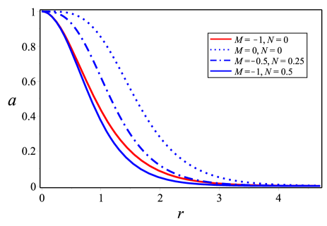
Figure 2: The profiles of the gauge field $a(r)$ for $n=1$. The red lines represent the solutions for a $|\phi|^{4}$ potential and blue lines for $|\phi|^{6}$ potentials.

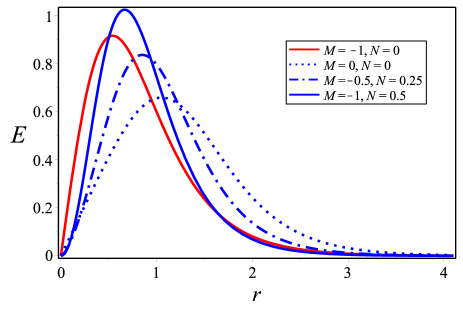
Figure 3: The profiles of the electric field $E(r)=A^{\prime}_{0}(r)$ for $n=1$. The red lines represent the solutions for a $|\phi|^{4}$ potential and blue lines for $|\phi|^{6}$ potentials.

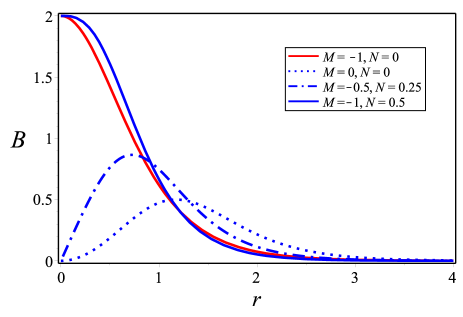
Figure 4: The profiles of the magnetic field $B(r)$ for $n=1$. The red lines represent the solutions for a $|\phi|^{4}$ potential and blue lines for $|\phi|^{6}$ potentials.

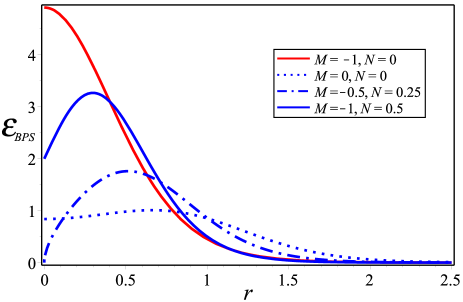
Figure 5: The profiles of the BPS energy density $\varepsilon_{{}_{bps}}(r)$ for $n=1$. The red lines represent the solutions for a $|\phi|^{4}$ potential and blue lines for $|\phi|^{6}$ potentials.

IV Remarks and conclusions

In summary, we have proposed a generalized abelian Chern-Simons-Higgs model with explicit breaking of Lorentz covariance and explored the respective Bogomolnyi framework. During the implementation of the BPS trick it is shown that the generalized functions should satisfy some requirements: The function $\omega(|\phi|)$ must be a monomial, i.e., $\omega=C|\phi|^{2\beta-2}$ for all $\beta\geq 1$ and the function $\omega_{1}(|\phi|)$ must be regular at the origin ($\omega_{1}\propto|\phi|^{2\delta}$ with $\delta\geq-1)$. Under such conditions imposed on the generalized functions, it is guaranteed the existence of self-dual solitonic configurations satisfying Bogomolnyi equations whose magnetic field and BPS energy density are well behaved. As we expected, the infinity family of self-dual configurations have finite energy which is proportional to the magnitude of the magnetic flux. In particular, we have studied the self-dual vortices provided by the choice $\omega_{1}(|\phi|)=\left(N+1\right)~{}|\phi|^{2N}$ and $\omega_{1}(|\phi|)=|\phi|^{2M}$. It was shown the vortex solutions of the Maxwell-Higgs model and the Chern-Simons-Higgs model can be also obtained. Besides that, we have constructed two new solitonic solutions which correspond to Chern-Simons theory coupled to two types of $|\phi|^{6}$ potentials given by Eqs. (54) and (55), respectively.

Finally, it is worthwhile to point out that existence of BPS states is linked to the existence of a $\mathcal{N}=2$-extended supersymmetric model WittenOlive . We are studying such a possibility despite the fact that in this model the Lorentz symmetry is explicitly broken. Advances in this direction will be reported elsewhere.

Conflict of Interests

The authors declare that there is no conflict of interests regarding the publication of this paper.

References

• (1) S. K. Paul, A. Khare, Phys. Lett. B174, 420 (1986) [Erratum-ibid. 177B, 453 (1986)].
• (2) H. J. de Vega, F. A. Schaposnik, Phys. Rev. D34, 3206 (1986).
• (3) R. Jackiw and S. Y. Pi, Prog. Theor. Phys. Suppl. 107, 1 (1992).
• (4) G. V. Dunne, Self-Dual Chern Simons Theories, Lecture Notes in Physics, m36, 1995, Springer.
• (5) G. V. Dunne, [arXiv:hep-th/9902115].
• (6) F. A. Schaposnik, [arXiv:hep-th/0611028].
• (7) P. A. Horvathy, P. Zhang, Phys. Rept. 481, 83 (2009).
• (8) R. Jackiw, E. J. Weinberg, Phys. Rev. Lett. 64, 2234 (1990).
• (9) J. Hong, Y. Kim, P. Y. Pac, Phys. Rev. Lett. 64, 2230 (1990).
• (10) R. Jackiw, S. Y. Pi, Phys. Rev. Lett. 64, 2969 (1990).
• (11) R. Jackiw, S. Y. Pi, Phys. Rev. D 42, 3500 (1990); Erratum-ibid. D 48, 3929 (1993).
• (12) E. Bogomolyi, Sov. J. Nucl. Phys 24, 449 (1976).
• (13) H. de Vega, F .A. Schaposnik, Phys. Rev. D14, 1100 (1976).
• (14) C. Lee, K. Lee, E. J. Weinberg, Phys. Lett. B243, 105 (1990).
• (15) R. Jackiw, Ki-Myeong Lee, E. J. Weinberg, Phys. Rev. D42, 3488 (1990).
• (16) T. H. R. Skyrme, Proc. Roy. Soc. A262, 237 (1961).
• (17) C. Armendariz-Picon, T. Damour and V. Mukhanov, Phys. Lett. B458, 209 (1999).
• (18) C. Armendariz-Picon, V. Mukhanov, P. J. Steinhardt, Phys. Rev. Lett. 85, 4438 (2000).
• (19) C. Armendariz-Picon, V. Mukhanov, Paul J. Steinhardt, Phys. Rev. D63, 103510 (2001).
• (20) T. Chiba, T. Okabe, M. Yamaguchi, Phys. Rev. D62, 023511 (2000).
• (21) M. Malquarti, E. J. Copeland, A. R. Liddle, Phys. Rev. D68, 023512 (2003).
• (22) J. U. Kang, V. Vanchurin, S. Winitzki, Phys. Rev. D76, 083511 (2007).
• (23) E. Babichev, V. Mukhanov, A. Vikman, J. High Energy Phys. 02, 101 (2008).
• (24) A. Sen, JHEP 0207, 065 (2002).
• (25) N. Arkani-Hamed, H.-C. Cheng, M. A. Luty, S. Mukohyama, JHEP 0405, 074 (2004).
• (26) N. Arkani-Hamed, P. Creminelli, S. Mukohyama, M. Zaldarriaga, JCAP 0404, 001 (2004).
• (27) S. Dubovsky, JCAP 0407, 009 (2004).
• (28) D. Krotov, C. Rebbi, V. Rubakov, V. Zakharov, Phys.Rev. D71, 045014 (2005).
• (29) A. Anisimov, A. Vikman, JCAP 0504, 009 (2005).
• (30) V. Mukhanov and A. Vikman, J. Cosmol. Astropart. Phys. 02, 004 (2006).
• (31) C. Armendariz-Picon and E. A. Lim, J. Cosmol. Astropart. Phys. 08, 007 (2005).
• (32) D. Bazeia, E. da Hora, C. dos Santos, R. Menezes, Phys. Rev. D81, 125014 (2010).
• (33) D. Bazeia, E. da Hora, R. Menezes, H. P. de Oliveira, C. dos Santos, Phys. Rev. D81, 125016 (2010).
• (34) C. dos Santos, E. da Hora, Eur. Phys. J. C70, 1145 (2010);
• (35) C. dos Santos, E. da Hora, Eur. Phys. J. C71, 1519 (2011).
• (36) C. dos Santos, Phys. Rev. D82, 125009 (2010).
• (37) D. Bazeia, E. da Hora, C. dos Santos, R. Menezes, Eur. Phys. J. C71, 1833 (2011).
• (38) D. Bazeia, R. Casana, E. da Hora, R. Menezes, Phys. Rev. D85, 125028 (2012).
• (39) R. Casana, M. M. Ferreira, Jr., E. da Hora, Phys. Rev. D86 085034 (2012).
• (40) E. Babichev, Phys. Rev. D74, 085004 (2006).
• (41) E. Babichev, Phys. Rev. D77, 065021 (2008).
• (42) C. Adam, J. Sanchez-Guillen, A. Wereszczynski, J. Phys. A 40, 13625 (2007); Erratum-ibid. 42, 089801 (2009).
• (43) C. Adam, N. Grandi, J. Sanchez-Guillen, A. Wereszczynski, J. Phys. A41, 212004 (2008); Erratum- ibid. 42, 159801 (2009).
• (44) C. Adam, N. Grandi, P. Klimas, J. Sanchez-Guillen, A. Wereszczynski, J. Phys. A41, 375401 (2008).
• (45) C. Adam, P. Klimas, J. Sanchez-Guillen, A. Wereszczynski, J. Phys. A42, 135401 (2009).
• (46) Lucas Sourrouille, Mod. Phys. Lett. A30, 1501211 (2015).
• (47) Rodolfo Casana, Lucas Sourrouille, Mod. Phys. Lett. A29, 1450124 (2014).
• (48) Lucas Sourrouille, Phy. Rev. D87, 067701 (2013).
• (49) Lucas Sourrouille, Phy. Rev. D86, 085014 (2012).
• (50) E. Babichev, Phys. Rev. D74, 085004 (2006).
• (51) D. Bazeia, L. Losano, R. Menezes, J. C. R. E. Oliveira, Eur. Phys. J. C51, 953 (2007).
• (52) X. Jin, X. Li. and D. Liu, Classical Quantum Gravity 24, 2773 (2007).
• (53) H. B. Nielsen and P. Olesen, Nucl. Phys. B61 45 (1973).
• (54) E. Witten and D. Olive, Phys. Lett. B78, 97 (1978).