Arrow of time in dissipationless cosmology

Abstract

It is generally believed that a cosmological arrow of time must be associated with entropy production. Indeed, in his seminal work on cyclic cosmology, Tolman introduced a viscous fluid in order to make successive expansion/contraction cycles larger than previous ones, thereby generating an arrow of time. However, as we demonstrate in this letter, the production of entropy is not the only means by which a cosmological arrow of time may emerge. Remarkably, systems which are dissipationless may nevertheless demonstrate a preferred direction of time provided they possess attractors. An example of a system with well defined attractors is scalar-field driven cosmology. In this case, for a wide class of potentials (especially those responsible for inflation), the attractor equation of state during expansion can have the form $p\simeq-\rho$, and during contraction $p\simeq\rho$. If the resulting cosmology is cyclic, then the presence of cosmological hysteresis, $\oint p~{}dV\neq 0$ during successive cycles, causes an arrow of time to emerge in a system which is formally dissipationless. An important analogy is drawn between the arrow of time in cyclic cosmology and an arrow of time in an $N$-body system of gravitationally interacting particles. We find that, like the $N$-body system, a cyclic universe can evolve from a single past into two futures with oppositely directed arrows of time.

E-mail: varun@iucaa.ernet.in, shtanov@bitp.kiev.ua and atopor@rambler.ru

I Introduction

It is a common and widespread belief that an arrow of time is invariably associated with some form of dissipation and entropy production which usually characterize irreversible phenomena. While it is true that dissipative phenomena do give rise to a preferred orientation of time, we demonstrate in this letter that entropy production is not essential for the existence of time’s arrow, and that such an arrow can appear even if the equations describing cosmic evolution are dissipationless and therefore formally time reversible. Examples to support our argument arise from scalar-field driven cosmology which has relevance both for a cyclic universe (section II) and inflation (section III). In the case of the cyclic universe, an arrow of time emerges on account of the presence of hysteresis: $\oint pdV\neq 0$, evaluated for any expansion-contraction cycle. Here, $p$ is pressure and $V$ is the volume of the universe. In this case, the increase $\delta a_{\rm max}$ in successive expansion maxima of the scale factor is related to the amount of hysteresis through $\delta a_{\rm max}^{n}=A\oint pdV$, where $n$ and $A$ depend upon the mechanism which causes the universe to turn around and contract in a given cycle.

We speculate that the presence of an arrow of time may be caused by the existence of attractors which single out one type of trajectory ($p\simeq-\rho$) during expansion and a different one ($p\simeq\rho$) during contraction. This behaviour is typical of inflationary potentials. In section II, we demonstrate that, while the scalar-field driven cyclic cosmology with hysteresis is stable, its time reversal possesses an instability. A similar instability with respect to time reversal also exists in the inflationary universe, discussed in section III. In section IV, we also draw attention to a curious similarity between the arrow of time in a cyclic universe and an arrow of time, recently discovered, in the gravitational clustering of dissipationless matter.

II Arrow of time in Cyclic Cosmology

Cyclic cosmology with dissipationless matter is usually not thought to possess an arrow of time. Indeed, if the Friedmann–Robertson–Walker (FRW) universe is spatially closed, then the Einstein equation

$$H^{2}=\kappa\rho-\frac{k}{a^{2}}\,,\qquad\kappa=\frac{8\pi G}{3}~{},$$ (1)

with $k=1$ leads to the following cyclic solution for pressureless matter

$$a(\eta)=A(1-\cos\eta)\,,\qquad t=A(\eta-\sin\eta)\,.$$ (2)

where $\eta=\int dt/a(t)$.

Figure 1: The expansion factor of a spatially closed matter-dominated universe is described by the self-similar cycloid shown above.

Solution (2), depicted in figure 1, has an initial singularity at $a=0$, which is periodically repeated. This singularity is absent in several modified-gravity theories. For instance, in a class of braneworld models yuri ; Maeda:2007cb and also in loop quantum cosmology (LQC) Ashtekar:2006uz ; Calcagni:2004wu ; Copeland:2005xs ; Singh:2006sg ; Stachowiak:2006uh , one gets

$$H^{2}=\kappa\rho\left\{1-\frac{\rho}{\rho_{c}}\right\}-\frac{k}{a^{2}}\,,\qquad\kappa=\frac{8\pi G}{3}\,,$$ (3)

which ensures that the universe ‘bounces’ when $\rho\simeq\rho_{c}$. At late times, when $\rho\ll\rho_{c}$, equation (3) reduces to (1). The value of $\rho_{c}$ is related to the fundamental parameters appearing in braneworld cosmology/LQC. We do not write them explicitly since the precise form of $\rho_{c}$ will not be required in this paper.

In an attempt to describe a cyclic universe with progressively larger cycles, Tolman tolman assumed the presence of a viscous fluid with pressure

$$p=p_{0}-3\zeta H\,,$$ (4)

where $p_{0}$ is the equilibrium pressure, $H={\dot{a}}/{a}$, and $\zeta$ is the coefficient of bulk viscosity. From equation (4) one finds that $p<p_{0}$ during expansion ($H>0$), whereas $p>p_{0}$ during contraction ($H<0$). This asymmetry during the expanding and contracting phases results in the growth of both energy and entropy. The increase in entropy makes the amplitude of successive expansion cycles larger, leading to a progressively larger and older universe tolman .

Tolman believed that thermodynamically recycling the universe would have a “liberalizing action on our general thermodynamic thinking” since it would dispel the notion that “the principles of thermodynamics necessarily require a universe which was created at a finite time in the past and which is fated for stagnation and death in the future” tolman . Thus Tolman’s oscillating universe presented an alternative to the idea of the thermodynamic heat death postulated by nineteenth century physicists and popular in the twentieth century as well.

Although Tolman linked the asymmetry in pressure during expansion and collapse to dissipation via (4), such an asymmetry arises even for non-dissipative systems such as a massive scalar field in an FRW space-time.

The energy density and pressure of a homogeneous scalar field are, respectively,

$$\rho=\frac{1}{2}\dot{\phi}^{2}+V(\phi)\,,\qquad p=\frac{1}{2}\dot{\phi}^{2}-V(\phi)\,,$$ (5)

and the scalar field equation of motion is

$$\ddot{\phi}+3H\dot{\phi}+\frac{dV}{d\phi}=0\,.$$ (6)

The term $3H\dot{\phi}$ in (6) acts like friction and damps the motion of the scalar field when the universe expands ($H>0$). By contrast, in a contracting ($H<0$) universe, the term $3H\dot{\phi}$ acts like anti-friction and accelerates the motion of the scalar field. Consequently, a scalar field with the potential $V=m^{2}\phi^{2}$ displays two attractor regimes belinsky1 ; belinsky2 ; belinsky3 ; kofman

$$\begin{array}[]{lll}p\simeq-\rho&\mbox{during expansion}&(H>0)\,,\\ p\simeq\rho&\mbox{during contraction}&(H<0)\,,\end{array}$$ (7)

which are depicted in figure 2. In cyclic cosmology, these two regimes combine together to produce cosmological hysteresis kanekar ; lesha , which is shown in figure 3.

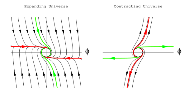
Figure 2: The attractor during expansion is ${\dot{\phi}}^{2}\ll V\Rightarrow p\simeq-\rho$, whereas during contraction the attractor is ${\dot{\phi}}^{2}\gg V\Rightarrow p\simeq\rho$; from kofman (figure Copyright 2002 by the American Physical Society). In a cyclic universe, these two attractor regimes give rise to cosmological hysteresis which is shown in figure 3.

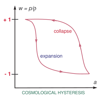
Figure 3: The hysteresis loop has $\oint pdV<0$ evaluated over a single expansion-contraction cycle in a scalar field dominated universe lesha (figure Copyright 2012 by the American Physical Society).

Figure 4: The presence of hysteresis, shown in figure 3, increases the amplitude of successive expansion maxima and endows a cyclic universe with an arrow of time. In the upper panel, cosmic turnaround is caused by the presence of a negative cosmological constant and the relevant expression linking the increase in successive expansion cycles to hysteresis is (10). In the lower panel, turnaround is due to the (positive) curvature term in (1). In this case the expression describing increasing expansion cycles is (8). In both panels the cyclic universe is sourced by a homogeneous scalar field with the potential $V(\phi)=\frac{1}{2}m^{2}\phi^{2}$; also see lesha .

Cosmological hysteresis is a remarkable feature which the scalar field shares with a viscous fluid by virtue of the parallel between (7) and (4). The system of equations (3), (5), (6) was numerically solved in kanekar ; lesha , and the results are summarized in figure 4. One finds that the presence of hysteresis leads to local time asymmetry in cyclic cosmology, which is reflected in the increase in amplitude of successive expansion cycles. This increase is related to the amount of hysteresis in a given cycle, namely $\oint pdV$. If cosmic contraction is sourced by the $k/a^{2}$ term in (3), then the increase in successive expansion maxima is given by kanekar ; lesha

$$\delta a_{\rm max}=-\kappa\oint pdV~{},$$ (8)

where $\oint pdV<0$. Because of the relation $\Omega-1=(aH)^{-2}$, the phenomenon of hysteresis leads to a universe which progressively becomes older, larger and more spatially flat with each successive cycle. In addition, cosmological hysteresis ensures that, for a potential such as $m^{2}\phi^{2}$, the inflaton field $\phi$ gets driven to larger values at the commencement of each new cycle. This ensures that the universe will ultimately inflate, even if it did not do so initially. Thus inflation can commence from a larger class of initial conditions in the presence of hysteresis than in its absence kanekar ; lidsey .

Note that the universe can turnaround and contract even in the absence of the curvature term provided its energy density can assume negative values. This can be accomplished in a number of ways: (i) Scalar-field potentials such as $V(\phi)=\lambda\phi^{4}-m^{2}\phi^{2}$ and $V(\phi)\propto\cos{\phi}$ permit $V(\phi)$ to evolve to negative values as the universe expands, leading eventually to contraction. (ii) A phantom field ($w<-1$) can give rise to a cyclic universe freese within the framework of the braneworld/LQC equation (3). (iii) The presence of a small negative cosmological constant, $\Lambda<0$, can make the universe turn around and contract, giving rise to cyclicity. In this case, the field equations become

$$H^{2}=\kappa\rho\left\{1-\frac{\rho}{\rho_{c}}\right\}-\frac{|\Lambda|}{3}\,,\qquad\kappa=\frac{8\pi G}{3}\,,$$ (9)

and the increase in successive expansion maxima is related to the quantum of hysteresis by

$$\delta a^{3}_{\rm max}=\frac{\kappa}{\Lambda}\oint pdV\,.$$ (10)

The hysteresis equations (8), (10) are quite robust, and follow simply from the relationship $\delta M+p\delta V=0$ (where $M=\rho a^{3}$), which is easily derived from the conservation condition $\nabla_{a}T^{a}{}_{b}=0\Rightarrow{\dot{\rho}}+3H(\rho+p)=0$.

Consider next an arbitrary trajectory $a(t)$, $\phi(t)$ of the cosmological system described by (3), (5), (6) with $k=1$. Since the scale factor is bounded from below by $a^{2}\geq 4/\kappa\rho_{c}$, there is, typically, a point on this trajectory where it reaches the minimal value $a=a_{\rm min}>0$. In our simulations, we always observe one such point at which the universe attains its smallest size. The neighborhood of this point can then be viewed as the “origin” of the arrow of time for this particular evolution. From this moment of time, the universe evolves with hysteresis and with systematically increasing scale factor in both time directions. We illustrate this U-shaped behaviour by the black (thin) curve in figure 5.

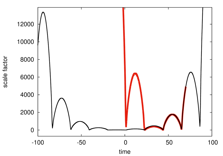
Figure 5: The expansion factor of a cyclic universe filled with a massive scalar field and evolved according to (3), (5), (6). The black (thin) curve is obtained by specifying a priori initial conditions at $t=0$ and integrating forward and backward in time. One finds that the expansion factor evolves to larger values in both time directions indicating that cosmological hysteresis is incremental ($\delta a_{\rm max}>0$) in both cases. The red (thick) curve is obtained by adding a small amount of noise (at the relative level of $10^{-6}$) to the phase space variables at $t=70$ and integrating backwards in time from this point. In this case the trajectory retraces its steps from $t=70$ to $t\simeq 20$ displaying decremental hysteresis ($\delta a_{\rm max}<0$) during this period. However after the first few cycles the expansion factor rapidly deviates from its original form and starts showing incremental hysteresis ($\delta a_{\rm max}>0$). The behaviour of the red (thick) curve thus illustrates that the scalar-field dominated universe with decremental hysteresis is unstable to small perturbations. In this simulation, we express all dimensional variables using reduced Planck units with mass scale $M_{*}=\sqrt{3/8\pi}M_{\rm P}$, where $M_{\rm P}=1/\sqrt{G}$ is the Planck mass, and we have chosen $m=3.5$, $\rho_{c}=60$, which corresponds to the physical parameters $m\approx 1.2\,M_{\rm P}$ and $\rho_{c}\approx 0.85\,M_{\rm P}^{4}$. The initial conditions are chosen to be $\phi=0.1$, $\dot{\phi}=-0.5$, and $a=5$. We should add, however, that the qualitative behaviour of the expansion factor shown above is generic and is common to a large class of initial conditions.

The above description suggests that the scale factor provides us with a natural arrow of time. The reason behind this lies in the fact that $a$ is the only variable in our phase space that is unbounded and unconstrained from above. In contrast, both the scalar field $\phi$ and its time derivative $\dot{\phi}$ are bounded by the condition $\rho\leq\rho_{c}$ valid for our system (3). The three-dimensional phase-space of our system, $\{a,\phi,{\dot{\phi}}\}$, can therefore be compared to a particle moving in a semi-infinite curved pipe whose one end is blocked by a wall. Bouncing back and forth off the walls of the pipe, the particle will typically move further and further away from the wall. Likewise, our system typically escapes to $a\to\infty$ as time goes on (in both time directions), under the joint influence of cyclicity and hysteresis.

It is interesting that the ‘one-past–two-futures’ behaviour encountered here has also been observed for an $N$-body system consisting of dissipationless particles interacting via Newtonian gravity Barbour:2013jya ; Barbour:2014bga . We discuss some similarities between our system and gravitational clustering in section IV.

Issues relating to the stability of trajectories

To obtain a U-shaped trajectory such as the black (thin) curve in figure 5, we start with some initial conditions at $t=0$ and evolve the system both to the past and to the future of this moment. In all cases that we have studied, with a priori initial conditions at $t=0$, we observe that the point of minimal value of the scale factor lies quite close to the moment $t=0$, and incremental hysteresis ($\delta a_{\rm max}>0$) quickly develops (after one or two cycles) in both time directions. In other words, by choosing the initial conditions at random, it appears to be quite improbable to fall on a trajectory that displays decremental hysteresis ($\delta a_{\rm max}<0$) for a considerable number of cycles. The only way to actually produce such a behavior is to time-reverse the trajectory with the usual incremental hysteresis ($\delta a_{\rm max}>0$). Thus, as we run the simulation shown by the black (thin) curve in figure 5 from $t=70$ backwards in time with the time-reversed initial conditions at $t=70$, we follow exactly the same evolution in reverse order, which, therefore, initially displays decremental hysteresis.

However, it is interesting to note that evolution in the direction of decremental hysteresis is unstable with respect to small variations in the initial conditions. We demonstrate this by perturbing the values of the phase-space variables at $t=70$ at the small relative level of $10^{-6}$ and running the simulation backwards in time from this point. In this case, we follow the trajectory shown by the red (thick) curve in figure 5. After a couple of cycles, this (red) trajectory begins to deviate from its original (black) trajectory and soon enters the regime of incremental hysteresis. In marked contrast to this behaviour, evolution in the direction of incremental hysteresis, when subject to similar perturbations, demonstrates perfect stability.

All this appears to suggest that we may be witnessing a phenomenon which, in some sense, is “physically” irreversible, meaning that reversibility is lost in the presence of even tiny perturbations. (This is similar to the process of statistical equilibration in a mechanical system with many degrees of freedom.) One may wonder about the reasons behind the time irreversibility displayed by our system. We believe that it is related to the different nature of its attractors during expansion and contraction. We have seen earlier that, for scalar-field driven cosmology, the equation of state of an attractor during expansion, $p\simeq-\rho$, is replaced by $p\simeq\rho$ during contraction (see figure 2). The stable inflationary regimes during expansion lead to an ever increasing size of the universe with each cycle, and therefore to incremental hysteresis. On the contrary, deflationary regimes during contraction (which would be responsible for decremental hysteresis) are highly unstable. Hence, they are improbable, and this is the reason why it is so unlikely to observe decremental hysteresis with a priori initial conditions. We stress here that the time irreversibility which we have encountered is manifest on sufficiently long timescales, involving several expansion-contraction cycles of the universe.

III Inflation

As demonstrated above, the cyclic universe appears to possess an arrow of time which may be related to the fact that stable trajectories become unstable under time reversal. Another example of a dissipationless system with similar properties (with respect to time reversal) is provided by inflation. The equation of motion (6) of the inflaton field is very similar to the motion of a body falling under gravity in a viscous medium characterized by a viscosity coefficient $\eta$:

$$m{\ddot{z}}+\eta{\dot{z}}-mg=0\,.$$ (11)

In both cases, an attractor is soon reached. In the case of (11), this attractor is the terminal velocity $v\equiv{\dot{z}}=mg/\eta$. It is reached by means of the transfer of translational energy of the body to the large number of translational and rotational degrees of freedom present in (molecules of) the viscous medium. This transfer results in an entropy increase, which converts the free-fall of the body into an irreversible process.

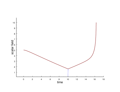
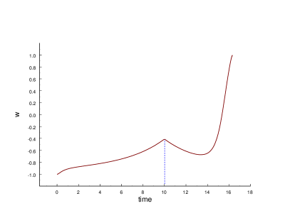
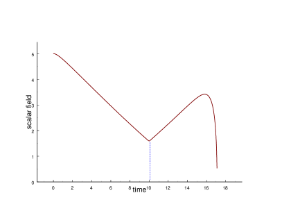
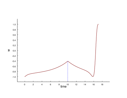
Figure 6: Scalar-field values (left) and the associated equation of state $w=p/\rho$ (right) for a universe undergoing inflation via the potential $V=m^{2}\phi^{2}/2$. (Units are in terms of the Planck scale.) The trajectory of $a(t)$, $\phi(t)$ is reversed at $t\simeq 10$ via ${\dot{\phi}}\to-{\dot{\phi}}$, $H\to-H$ (vertical blue line) by simultaneously perturbing $H$ by $10^{-4}$ (upper panel) and $10^{-6}$ (lower panel) of its original value. Since the equations of motion are time-reversible, one might expect the time-reversed trajectory at $t>10$ to be a mirror image of the forward-time trajectory at $t<10$. Surprisingly, this is not the case. For a while after time reversal ($10\leq t\leq 14$), $\phi(t)$ does follow its forward time evolution ‘backward in time’, with $w$ decreasing as expected. But for $t>14$ the time-reversed trajectory becomes highly unstable causing $w$ to increase towards $+1$ instead of decreasing to $-1$.

Similarly, a scalar field rolling down a potential with a gentle slope soon reaches the slow-roll limit: $|{\dot{\phi}}|\simeq|V^{\prime}/3H|$, $|{\ddot{\phi}}|\ll|3H\dot{\phi}|$. In this case, the role of viscosity is played by the expansion of the universe, so that $\eta\equiv 3H$. An important difference from (11) is that, since equation (6) is not associated with microscopic entropy production, the universe precisely follows its time-reversed trajectory after the signs of $H$ and ${\dot{\phi}}$ have been reversed. However, after time reversal, the Hubble parameter changes sign, which makes the second term in (6), which originally acted like friction, to behave like anti-friction, rendering the time-reversed slow-roll trajectory unstable to small perturbations. Since small perturbations, in the form of quantum fluctuations, are always present in the inflationary scenario, one comes to the conclusion that, practically speaking, an inflationary trajectory is difficult to reverse, as illustrated in figure 6. As shown in that figure, a larger perturbation causes, upon time reversal, an earlier departure from the inflationary equation of state $w\simeq-1$. Moreover, one sees that the perturbation in the left panel of figure 6 (in which the Hubble parameter has been perturbed by $10^{-4}$ times its original value) leads to the asymptotic behaviour $\phi\to+\infty$, whereas perturbing the time derivative of the scale factor by $10^{-6}$ of its original value induces the $\phi\to-\infty$ regime. In a more realistic scenario involving inhomogeneous perturbations, a rapid deviation from the inflationary regime would be accompanied by growth in scalar-field inhomogeneity. This issue, however, lies beyond the scope of the present paper.

The departure from the inflationary regime during contraction leads to a larger value of the scale factor as the Planck density is reached. Consequently, in the presence of a hypothetical Planck-scale bounce, the next cycle commences from a larger value of the scale factor than the previous one, as shown in figure 5. (This happens because the energy density, $\rho_{\phi}$, varies slowly near the de Sitter regime but grows much more rapidly: as $a^{-6}$, during the asymptotic $w\simeq 1$ stage of expansion displayed in the right panel of figure 6).

The fact that the inflationary trajectory is difficult to reverse has important consequences.

It is well known that the homogeneous and isotropic FRW universe, in which matter satisfies the ‘energy conditions’, comprises a set of measure zero in the space of all homogeneous but anisotropic solutions of the Einstein equations ch73 . Taken at face value, this might suggest that the universe unravelled from a very special set of initial conditions. However, the inflationary paradigm throws a fresh perspective on this issue since, an anisotropic universe containing a positive cosmological constant rapidly isotropises, approaching the de Sitter space attractor if the spatial curvature is not too large no-hair . This remains true for inflationary space-times in which a scalar field replaces $\Lambda$ ms86 ; no-hair1 . In this case, the de Sitter space attractor solution is a transient, and lasts while the slow roll conditions are satisfied. Consider, for instance, the Bianchi I model

$$ds^{2}=dt^{2}-\sum_{i=1}^{3}a_{i}^{2}(t)(dx^{i})^{2}\,,$$ (12)

for which the equations of motion become

$$H^{2}=\frac{8\pi G}{3}\rho+\frac{1}{2}{\dot{\phi}}^{2}+V(\phi)+\rho_{\rm anis}~{},$$ (13)

$$\ddot{\phi}+3H\dot{\phi}+\frac{dV}{d\phi}=0~{},$$ (14)

where $H$ describes the mean expansion rate

$$H=\frac{1}{3}\sum_{i=1}^{3}\left(\frac{{\dot{a}_{i}}}{a_{i}}\right)=\frac{\dot{a}}{a}~{},\qquad a=\left(a_{1}a_{2}a_{3}\right)^{1/3}~{},$$ (15)

and the anisotropy is encoded in the anisotropy density $\rho_{\rm anis}$ :

$$\rho_{\rm anis}=\frac{1}{6}\sum_{i=1}^{3}\left(\frac{{\dot{a}_{i}}}{a_{i}}-H\right)^{2}=\frac{\Sigma}{a^{6}}~{}.$$ (16)

From (13) we see that a large initial anisotropy, $\rho_{\rm anis}$, increases the expansion rate, $H$, thereby introducing greater damping into the scalar field equation of motion (14). The inflationary attractor $P\simeq-\rho$ in (7) can therefore be more rapidly reached in the presence of anisotropy than in its absence ms86 ; maartens . The observation that inhomogeneities and anisotropies get rapidly diluted in an inflationary universe has occasionally been referred to as the ‘cosmic no-hair theorem’ in analogy with no-hair theorems for black holes proven during the 1970’s.

However, the fact that the equations governing inflationary expansion are reversible has sometimes been used to undermine the no-hair theorem by means of the following argument. Let us consider a hypothetical universe, far more anisotropic than ours, in which the present anisotropy parameter is $\rho^{\rm final}_{\rm anis}$. Then, since the equations of motion (13), (14) are reversible, one can evolve them back in time in order to determine the initial anisotropy, $\rho^{\rm initial}_{\rm anis}$, which would have led to $\rho^{\rm final}_{\rm anis}$ after inflation. In this manner, it is always “possible to choose initial data in such a way that the universe would be more anisotropic than ours is today” ms86 . The weakness in this argument is connected with the issue of the probability of such initial conditions. In the previous section, we demonstrated that randomly chosen a priori initial conditions always lead to incremental hysteresis, hence, develop an arrow of time from the very beginning. If the conditions leading to decremental hysteresis are indeed quite improbable, then the presence of small perturbations (in the form of vacuum fluctuations) makes the equations of motion of the scalar field effectively non-reversible. This observation considerably weakens the above argument and strengthens the no-hair theorem. (We propose to study this issue in greater detail in a companion work.)

IV Discussion

We have demonstrated the appearance of an arrow of time in the time-reversible cosmological system consisting of a spatially closed universe filled with a homogeneous scalar field. This situation is not uncommon, and takes place in statistical physics with many degrees of freedom, where, for example, the (classical) molecular dynamics is evidently reversible, but small deviations from the exact time-reversed velocities (which would lead to an evolution with decreasing entropy) rapidly lead to the usual entropy increase. In the case of cyclic cosmology, the presence of an arrow of time is intimately linked to the phenomenon of hysteresis. Four important conditions need to be satisfied for the occurrence of hysteresis:

1. The potential for $V(\phi)$ should allow the occurrence of inflation.

2. $V(\phi)$ should have a minimum about which the scalar field oscillates after inflation. This condition is essential since it allows the field $\phi$ to phase-mix. When this condition is relaxed, for instance in monotonically decreasing potentials such as $V(\phi)\propto\phi^{\alpha},\,\alpha<0$, hysteresis is absent and all cycles have the same amplitude lesha .

3. A condition for turnaround is present, either in the form of positive spatial curvature or a negative cosmological constant, or a potential $V(\phi)$ which becomes negative at late times.

4. The initial big-bang singularity is replaced by a bounce at large densities.

If the above conditions are met, then the FRW cosmology of a scalar field with a priori initial conditions exhibits an arrow of time, with preferred evolution towards larger scale factors from cycle to cycle. Phenomenologically, the dissipationless universe with a scalar field behaves as if it contained a fluid with bulk viscosity, with the asymmetry in pressure during expansion and contraction giving rise to the phenomenon of cosmological hysteresis.

One should mention here that an arrow of time has also been discovered quite recently in the very different context of Newtonian dynamics Barbour:2013jya ; Barbour:2014bga . It was noticed that an $N$-body system of point masses with Newtonian gravitational attraction can be endowed with a specific quantity, called complexity by the authors, whose value reaches a minimum on every $N$-body trajectory with total centre-of-mass energy and total angular momentum both equal to zero. Complexity is given by the ratio $C_{\rm S}=\ell_{\rm rms}/\ell_{\rm mhl}$, where

$$\ell_{\rm rms}=\frac{1}{m_{\rm tot}}\left(\sum_{a<b}m_{a}m_{b}r_{ab}^{2}\right)^{1/2}=\left(\frac{I_{\rm cm}}{m_{\rm tot}}\right)^{1/2}$$ (17)

is the root-mean-square length, which is expressed through the centre-of-mass moment of inertia $I_{\rm cm}$, and the mean harmonic length $\ell_{\rm mhl}$ is defined by

$$\frac{1}{\ell_{\rm mhl}}=\frac{1}{m_{\rm tot}^{2}}\sum_{a<b}\frac{m_{a}m_{b}}{r_{ab}}\,.$$ (18)

Complexity displays a U-shaped behaviour since its value systematically decreases before the minimum point and systematically increases after it. This quantity can thus play the role of an entropy, and the point of its minimum can be regarded as a point where the arrow of time changes direction. We encountered this U-shaped ‘one-past–two-futures’ behaviour earlier, in section II, in our discussion of hysteresis. We elaborate on this issue once more, in view of its importance, since it has appeared in two completely distinct discussions of the arrow of time.

The black (thin) curve in Figure 5 shows a typical trajectory in terms of the scale factor. There is a point around $t=0$ where the scale factor takes a minimal value.

As we move from $t=0$ to the past or to the future, the universe displays hysteresis in both time directions. However, when the trajectory is viewed in one time direction, say, from left to right, it is unstable in the region $t<0$ (decremental hysteresis, $\delta a_{\rm max}<0$), while it is stable in the region $t>0$ (incremental hysteresis, $\delta a_{\rm max}>0$).

There are several conclusions that one can derive from this picture.

• A typical evolution of the universe in our model possesses hysteresis and an “origin of time” (region around $t=0$), from which the evolution is similar in both time directions.

• The trajectories are stable in the direction of time which displays incremental hysteresis ($\delta a_{\rm max}>0\Rightarrow\oint pdV<0$), and are unstable in the opposite direction.

• All these features are quite similar to the behaviour of entropy. If we prepare a complicated physical system (a gas in a box) randomly distributed and in a non-equilibrium state and run it in both time directions, we will observe an entropy increase in both time directions. The system will tend to thermodynamic equilibrium in both time directions, and this convergence to equilibrium will be stable with respect to perturbations of initial conditions. However the time-reversed evolution in both cases will be highly unstable.

We have thus demonstrated that our cyclic model possesses the U-shaped ‘one-past–two-futures’ behaviour discovered recently for an $N$-body system. The scalar-field based cyclic universe may therefore be regarded as the simplest known example of a dissipationless system possessing an arrow of time.

One should also note the similarity of the eternal classical universe depicted by the black (thin) curve in figure 5 to the scenario of eternal inflationary universe due to Carroll and Chen Carroll:2004pn . In the latter, it is a spontaneous quantum fluctuation in the scalar field in a vacuum de Sitter space that plays the role of the ‘origin’ of time, which then flows towards eternal inflation and entropy growth in two opposite directions. In our model, the universe is driven by a classical scalar field during all its history, and quantum fluctuations are not taken into account.

Finally, we draw attention to the fact that we do not consider spatial inhomogeneities in the present work. Introducing such inhomogeneities would mean increasing the number of degrees of freedom and creating new kinds of instability. The fact that inhomogeneities are growing during cosmological evolution creates the usual arrow of time for gravitating systems — a self-gravitating system evolves from a homogeneous to a highly nonhomogeneous distribution (in contrast to a molecular gas, which evolves towards a homogeneous configuration). The well-known proposal by Penrose to use the Weyl tensor as a measure of gravitational entropy is based on this property (see for instance Clifton for the current state of this proposal).

Our study demonstrates the existence of cosmological situations where the effective arrow of time is not associated with the Weyl tensor. This is so because this tensor identically vanishes for the FRW metric which we consider. This leads to the conclusion that not all effectively time-irreversible phenomena in self-gravitating systems can be reduced to measures based on the Weyl tensor (and, more generally, that there exist time-irreversible phenomena which are not associated with the growth of spatial inhomogeneities).

References

References

- (1) Shtanov Yu and Sahni V 2003 Phys. Lett. B 557 1–6
-
(2)
Maeda H, Sahni V and Shtanov Yu 2009
Phys. Rev. D 76 104028
Maeda H, Sahni V and Shtanov Yu 2009 Phys. Rev. D 80 089902 (erratum) - (3) Ashtekar A, Pawlowski T and Singh P 2006 Phys. Rev. D 73 124038
- (4) Calcagni G 2005 Phys. Rev. D 71 023511
- (5) Copeland E J, Lidsey J E and Mizuno S 2006 Phys. Rev. D 73 043503
- (6) Singh P 2006 Phys. Rev. D 73 063508
- (7) Stachowiak T and Szydłowski M 2007 Phys. Lett. B 646 209–214
- (8) Novello M and Perez Bergliaffa S E 2008 Phys. Rep. 463 127–213
- (9) Tolman R C 1934 Relativity, Thermodynamics and Cosmology (Oxford: Clarendon) p 524
- (10) Belinsky V A, Grishchuk L P, Khalatnikov I M and Zeldovich Ya B 1985 Sov. Phys.—JETP 63 195–203
- (11) Belinsky V A, Khalatnikov I M, Grishchuk L P and Zeldovich Ya B 1985 Phys. Lett. B 155 232–236
- (12) Belinsky V A, Ishihara H, Khalatnikov I M and Sato H 1988 Prog. Theor. Phys. 79 676–684
- (13) Felder G N, Frolov A V, Kofman L and Linde A D 2002 Phys. Rev. D 66 023507
- (14) Kanekar N, Sahni V and Shtanov Yu 2001 Phys. Rev. D 63 083520
- (15) Sahni V and Toporensky A 2012 Phys. Rev. D 85 123542
- (16) Lidsey J E, Mulryne D J, Nunes N J and Tavakol R 2004 Phys. Rev. D 70 063521
- (17) Brown M G, Freese K and Kinney W H 2008 JCAP 0803 002
- (18) Barbour J, Koslowski T and Mercati F 2013 A gravitational origin of the arrows of time Preprint arXiv:1310.5167 [gr-qc]
-
(19)
Barbour J, Koslowski T and Mercati F 2014 Phys. Rev. Lett. 113 181101
Barbour J, Koslowski T and Mercati F 2014 Entropy and the typicality of universes Preprint arXiv:1507.06498 [gr-qc] - (20) Collins C B and Hawking S W 1973 Astrophys. J. 180 317–334
-
(21)
Hoyle F and Narlikar J V 1963 Proc. Roy. Soc. A 273 1–11
Gibbons G W and Hawking S W 1977 Phys. Rev. D 15 2738–2751
Hawking S W and Moss I G 1982 Phys. Lett. B 110 35–38
Starobinsky A A 1983 Pis’ma Astron. Zh. 9 579–584
Starobinsky A A 1983 Sov. Astron. Lett. 10 302–304
Wald R W 1983 Phys. Rev. D 28 (1983) 2118–2120 - (22) Moss I and Sahni V 1986 Phys. Lett. B 178 159–162
-
(23)
Rothman T and Ellis G F R 1986 Phys. Lett. B 180 19–24
Jensen L G and Stein-Schabes J 1986 Phys. Rev. D 34 931–933
Turner M S and Widrow L M 1986 Phys. Rev. Lett. 57 2237–2240 - (24) Maartens R, Sahni V and Saini T D 2001 Phys. Rev. D 63 063509
-
(25)
Starobinsky A A 1978 Pis’ma Astron. Zh. 4 155–159
Starobinsky A A 1978 Sov. Astron. Lett. 4 82–84 - (26) Piao Y-S 2004 Phys. Rev. D 70 101302(R)
- (27) Carroll S M and Chen J 2004 Spontaneous inflation and the origin of the arrow of time Preprint arXiv:hep-th/0410270
- (28) Clifton T, Ellis G F R and Tavakol R 2013 Class. Quant. Grav. 30 125009