Initial data for rotating cosmologies

Abstract

We revisit the construction of maximal initial data on compact manifolds in vacuum with positive cosmological constant via the conformal method. We discuss, extend and apply recent results of Hebey et al. [19] and Premoselli [31] which yield existence, non-existence, (non-)uniqueness and (linearisation-) stability of solutions of the Lichnerowicz equation, depending on its coefficients. We then focus on so-called $(t,\varphi)$-symmetric data as “seed manifolds”, and in particular on Bowen-York data on the round hypertorus $\mathbb{S}^{2}\times\mathbb{S}$ (a slice of Nariai) and on Kerr-de Sitter. In the former case, we clarify the bifurcation structure of the axially symmetric solutions of the Lichnerowicz equation in terms of the angular momentum as bifurcation parameter, using a combination of analytical and numerical techniques. As to the latter example, we show how dynamical data can be constructed in a natural way via conformal rescalings of Kerr-de Sitter data.

1 Introduction

We start with two definitions.

Definition 1.

As Initial Data (ID) $(\widetilde{\cal M},\widetilde{g}_{ij},\widetilde{K}_{ij})$ (i,j,=1,2,3) for vacuum with positive cosmological constant $\Lambda$ we take a compact 3-dim. Riemannian manifold $\widetilde{\cal M}$ with smooth metric $\widetilde{g}_{ij}$ and smooth second fundamental form $\widetilde{K}_{ij}$ which is maximal $\widetilde{g}^{ij}\widetilde{K}_{ij}=0$ and satisfies the constraints

$$\widetilde{R}=\widetilde{K}_{ij}\widetilde{K}^{ij}+2\Lambda\qquad\widetilde{\nabla}_{i}\widetilde{K}^{ij}=0$$ (1)

Here $\widetilde{\nabla}$ and $\widetilde{R}$ are the covariant derivative and the scalar curvature of $\widetilde{g}_{ij}$.

Definition 2.

A Seed Manifold (SM) $({\cal M},g_{ij},K_{ij})$ consists of a compact 3-dim. manifold $({\cal M},g_{ij})$ with smooth metric in the positive Yamabe class, and of a smooth trace-free and divergence-free tensor $K_{ij}$ on ${\cal M}$.

The conformal method is the art of turning a SM into an ID via conformal rescaling [24]. In the present setting it remains to be shown that the Lichnerowicz equation

$$\Phi(\phi):=-\left(\Delta-\frac{1}{8}R\right)\phi-\frac{1}{4}\Lambda\phi^{5}-\frac{\Omega^{2}}{8\phi^{7}}=0$$ (2)

has a smooth, strictly positive solution $\phi$, where $\Delta$ and $R$ are the Laplacian and the scalar curvature of $g_{ij}$, and $\Omega^{2}=K^{ij}K_{ij}$. In this case the “physical” quantities

$$\widetilde{g}_{ij}=\phi^{4}g_{ij}\qquad\widetilde{K}^{ij}=\phi^{-10}K^{ij}$$ (3)

indeed satisfy the constraints (1).

In view of the observed small positive value of $\Lambda$, and due to the naturality of the assumption of maximality of the data, we are dealing here with a physically very realistic case of the Lichnerowicz equation. It is precisely this case, however, which involves rather intricate mathematical problems. Firstly, solutions definitely do not exist for large $\Omega^{2}$ which is rather easy to see in principle either from the maximum principle, or by integrating (2). On the other hand, existence proofs for small $\Omega^{2}$ are subtle, in particular when $\Omega^{2}$ is allowed to have zeros [18, 19, 20, 31]. However, in physically meaningful situations $\Omega^{2}$ does have zeros - in the axially symmetric (AS) case, on which we focus in this paper and which is simple in other respects, $\Omega^{2}$ in fact typically vanishes on the axis (cf. Sect. 3).

There are now available two types of general existence and non-existence results which cover the case of present interest. The first one, due to Hebey et al. [19] (see also [18, 20]) guarantees existence of solutions if $\int_{\cal M}\Omega^{2}$ is small, and proves non-existence if $\int_{\cal M}\Omega^{5/6}$ is large. In either case, the bounds can be given explicitly in terms of the Yamabe constant of ${\cal M}$ and other integrals over ${\cal M}$. However, there is a $\Omega$-“gap” which is not covered by these results. In the second theorem, due to Premoselli [31], $\Omega$ is written as $\Omega=b\,\Omega_{0}$ for some (fixed) function $\Omega_{0}$ and (variable) constant $b>0$, and the result is “gap free”: It is asserted that there is a constant $b_{\ast}\in(0,\infty)$ such that (2) has at least two positive solutions for all $b<b_{\ast}$, a unique solution for $b=b_{\ast}$ and no solution for $b>b_{\ast}$. Moreover, for every $b\leq b_{\ast}$ there is a unique stable, “minimal” solution. We remark, however, that in this theorem there is no direct information about $b_{\ast}$ in terms of more familiar geometric quantities of ${\cal M}$.

In this work we start (in Sect. 2.1) with defining (in Def. 3) (linearisation-) stability of solutions of (2) and of ID (under conformal deformations), which will be key in what follows. In particular we prove Proposition 1 which guarantees instability if $\widetilde{\Omega}^{2}=\widetilde{K}_{ij}\widetilde{K}^{ij}<\Lambda$. Another important issue in our work is “symmetry-inheriting” versus ”symmetry-breaking” of solutions, by which we mean solutions of (2) which share (or don’t share) all symmetries of the equation. In Sect. 2.2. we prove a simple result (Proposition 2) which ensures symmetry inheritance for stable solutions in the case of continuous symmetries. We proceed in Sect. 2.3. by reviewing the theorems of Hebey et al. and Premoselli mentioned above. As small complements to the latter result, we clarify (in Proposition 3) how the stable, minimal solutions of (2) approach zero as $b\rightarrow 0$. Moreover, in Proposition 4 we employ an argument from bifurcation theory to show that near the maximal value $b_{*}$, there are precisely two solutions.

The core of our paper is Sect. 3 where we apply the results sketched above to certain “$(t,\varphi)$-symmetric data” as introduced and discussed in [15, 16]. There one sets out from an AS “twist potential” $\omega$ from which there is constructed an AS, symmetric, trace-free and divergence free tensor $K_{ij}$. The SM constructed in this way “rotate” in general, and the (Komar-) angular momentum $J$ of any selected 2-surface is given directly in terms of the values of $\omega$ on the axis via $8\pi J=[\omega(0)-\omega(\pi)]$. We focus on two different classes of seed manifolds (${\cal M},g_{ij}$) as examples: In Sect. 3.3. we consider a “round hypertorus”, i.e. $\mathbb{S}^{2}\times\mathbb{S}^{1}$ with a round $\mathbb{S}^{2}$. We first review the case without angular momentum where the solutions of (2) yield the time symmetric Kottler (Schwarzschild-de Sitter) data. Then we consider a $K_{ij}$ of “Bowen-York form” [4, 6] as the simplest non-trivial rotating model. Applying the results of Hebey et al. [19] we find (in Theorem 3) that small angular momenta (compared to $\Lambda^{-1}$, and taken w.r.t. the $\mathbb{S}^{2}$ surfaces) guarantee existence of solutions of (2) while large ones exclude existence. Finally, we apply Premoselli’s theorem [31]. Combined with auxiliary results from bifurcation theory, with results on stability and symmetry collected in Sect 2., as well as with numerical methods, we are able to clarify the bifurcation structure of the axially symmetric solutions in terms of the bifurcation parameter $b=3J\Lambda/2$: Firstly, there is a pair of “principal” branches consisting of stable and unstable solutions all of which inherit the $O(2)\times O(2)$- symmetry of the SM. These branches emanate at $J=0$ from the solutions $\phi\equiv 0$ and $\phi\equiv 1$, respectively, and meet at some marginally stable solution $\phi_{*}$ corresponding to a maximal angular momentum $J_{*}$. Moreover, off certain points on the unstable principal branch there bifurcate branches which break the O(2)-symmetry along the $\mathbb{S}$ direction, and which terminate at the Kottler solutions in the limit of vanishing angular momentum. We summarize these facts as Conjecture 1, which also includes the hypothesis that there are no solutions which break the axial symmetry on $\mathbb{S}^{2}$.

In Sect. 3.4. we consider as SM the standard maximal slice of Kerr-de Sitter. For any fixed $\Lambda$, we take a family of $(t,\varphi)$-symmetric data generated by $\omega(r,\theta,\Lambda,J,a,m)=J\omega_{K}(r,\theta,\Lambda,a,m)/J_{K}$ where $\theta$ and $r$ are “Boyer-Lindquist” coordinates, $J$ is the “true” angular momentum and $\omega_{K}$ is the twist potential generating Kerr-de Sitter with angular momentum $J_{K}=ma(1+\Lambda a^{2}/3)^{-2}$ in terms of its standard parameters $m$ and $a$. This example is particularly well suited to illustrate Premoselli’s result [31]: Choosing $b=3J\Lambda/2$ as above, it trivially implies existence of solutions to (1) for all $J\leq J_{K}$. More interestingly, it also shows that Kerr-de Sitter can be “overspun” in the sense that there exist data with $J>J_{K}$ as long as they remain strictly unstable. The latter is guaranteed in particular by the criterium $\widetilde{\Omega}^{2}<\Lambda$ of Sect. 2.1. mentioned above, but in any case for sufficiently small $J_{K}$ and small $J-J_{K}$ (again compared to $\Lambda^{-1}$). These facts are collected in Theorem 4.

2 Stability, symmetry, existence and non-existence

2.1 Stability

In the following discussion we refer to SMs and IDs as defined in Defs. 1. and 2.. As a rule the metric and the second fundamental form of IDs will carry tildes. We note, however, that the SM in our examples (Sects 3.3. and 3.4.) trivially satisfy the constraints as well, so they are IDs on their own. Hence the task here is actually to generate non-trivial IDs from trivial ones.

We first define and discuss here (linearisation-) stability of solutions of (2) under conformal deformations, which will be crucial in the following results. The linearized operator $L_{\phi}$ corresponding to (2) applied to some function $\gamma$ reads

$$L_{\phi}\gamma:=-\left(\Delta-\frac{R}{8}\right)\gamma-\frac{5\Lambda}{4}\phi^{4}\gamma+\frac{7\Omega^{2}}{8\phi^{8}}\gamma$$ (4)

Definition 3.

1. A solution $\mathbf{\phi}$ of (2) on a SM $({\cal M},g_{ij},K_{ij})$ is called strictly stable, stable, marginally stable, unstable or strictly unstable if the lowest eigenvalue $\varsigma$ in (4) at $\phi$ satisfies $\varsigma>0$, $\varsigma\geq 0$, $\varsigma=0$, $\varsigma\leq 0$, or $\varsigma<0$, respectively.

2. ID given by Equ. (1) are said to have lowest eigenvalue $\varsigma$ (under conformal deformations) if (4) has this lowest eigenvalue at $\phi\equiv 1$. The ID are called strictly stable if $\phi\equiv 1$ is strictly stable, and analogous definitions for ID apply with the other stability properties.

The natural question raised by these definitions is resolved as follows.

Lemma 1.

A strictly stable solution $\phi$ of (2) on a SM $({\cal M},g_{ij},K_{ij})$ defines via (3) strictly stable ID $(\widetilde{\cal M},\widetilde{g}_{ij},\widetilde{K}_{ij})$. The same applies to the other stability properties of Definition 3.

Proof.

We show, more generally, that only the conformal class of the SM matters for stability of the solution of (2) and for the resulting ID. We first note that (2) is obviously conformally invariant in the sense that when $\phi$ solves (2) and defines ID $(\widetilde{\cal M},\widetilde{g}_{ij}=\phi^{4}g_{ij},\widetilde{K}_{ij}=\phi^{-2}K_{ij})$, then $\widehat{\phi}=\vartheta^{-1}\phi$ solves (2) on the SM $(\widehat{\cal M},\widehat{g}_{ij}=\vartheta^{4}g_{ij},\widehat{K}_{ij}=\vartheta^{-2}K_{ij})$ and defines the same ID. A conformal covariance property also holds for the linearisation operator (4) in the sense that the rescaling $\widehat{\gamma}=\vartheta^{-1}\gamma$ gives $\widehat{L}_{\widehat{\phi}}\widehat{\gamma}=\vartheta^{-5}L_{\phi}\gamma$ in terms of $\widehat{L}_{\widehat{\phi}}$ on $\widehat{\cal M}$. A subtlety now arises since the eigenvalue equation $L_{\phi}\mu=\lambda\mu$ is obviously not conformally invariant (when the eigenfunction $\mu$ is scaled as above) and the same applies to the eigenvalues themselves. However, what matters for stability is only the sign (or the vanishing) of the lowest eigenvalue $\varsigma$. To show that this is actually invariant we recall the Rayleigh-Ritz characterisation,

$$\varsigma=\inf_{\gamma\in C^{\infty},\gamma\not\equiv 0}\frac{\int_{\cal M}\gamma L_{\phi}\gamma dv}{\int_{\cal M}\gamma^{2}}$$ (5)

and note that its numerator is invariant, while the denominator is manifestly positive. The statement of the Lemma is now obtained by setting $\vartheta=\phi$ in the above arguments. ∎

Remarks.

1. Recalling that the eigenvalues $\lambda$ depend on the conformal scaling of the metric in general, we denote by $\widetilde{\lambda}$ the eigenvalues w.r.t to the generated ID (i.e. when $\phi\equiv 1$ in (4)).

2. The above definitions of stability under conformal deformations have nothing to do with dynamical stability of the solutions evolving from the data. We will return to this issue in connection with the Kerr-de Sitter example in Sect.3.4.

Proposition 1.

Let $(\widetilde{\cal M},\widetilde{g}_{ij},\widetilde{K}_{ij})$ be ID with volume $\widetilde{V}$ and lowest eigenvalue $\widetilde{\varsigma}$. Then

1. $$\int_{\widetilde{\cal M}}\widetilde{\Omega}^{2}d\widetilde{v}\geq(\Lambda+\widetilde{\varsigma})\widetilde{V}.$$ (6)

2. If $\widetilde{\Omega}^{2}\leq\Lambda$ and $\widetilde{\Omega}^{2}\not\equiv\Lambda$ on $\widetilde{\cal M}$, then the ID are strictly unstable.

3. If $\widetilde{\Omega}\equiv 0$, then $\widetilde{\varsigma}=-\Lambda$, while $\widetilde{\Omega}^{2}\equiv\Lambda$ implies $\widetilde{\varsigma}=0$.

Proof.

Combining (1) with (4) for $\phi\equiv 1$ we find

$$\widetilde{\Delta}\widetilde{\zeta}=(\widetilde{\Omega}^{2}-\Lambda-\widetilde{\varsigma})\widetilde{\zeta}$$ (7)

where $\widetilde{\zeta}$ is the eigenfunction corresponding to the lowest eigenvalue $\widetilde{\varsigma}$. As $\widetilde{\zeta}$ has no zeros it can be chosen to be positive. Dividing by $\widetilde{\zeta}$ and integrating, we obtain

$$\int_{\widetilde{\cal M}}(\widetilde{\Omega}^{2}-\widetilde{\zeta}^{-2}|\widetilde{\nabla}\widetilde{\zeta}|^{2})d\widetilde{v}=(\Lambda+\widetilde{\varsigma})\widetilde{V}$$ (8)

which implies assertions 1. and 2.. Point 3. is a consequence of the maximum principle applied to (7). ∎

Remark. We wish to clarify here an important point which arises by combining Lemma 1 with Proposition 1: These results do not imply that any solution of (4) with $\Omega$ small enough on a SM ${\cal M}$ leads to unstable ID $\widetilde{\cal M}$. Rather, the tilde on $\widetilde{\Omega}^{2}$ in the requirement $\widetilde{\Omega}^{2}=\phi^{-12}\Omega^{2}\leq\Lambda$ of Proposition 1 must not be overlooked. In fact, the stable examples with small $\Omega$ but large $\widetilde{\Omega}$ (and hence small $\phi$) will play a key role below.

2.2 Stability and symmetry

We recall from the introduction that “symmetry-inheriting” and “symmetry breaking” are the properties of solutions of (2) of (not) sharing all symmetries of the equation. This behaviour is related to (in-)stability of solutions; we will observe it in the Bowen-York example of Sect. 3.3.3. We note here the following

Proposition 2.

Assume that a SM $({\cal M},g_{ij})$ and $\Omega$ have a continuous symmetry $\xi$, i.e.

$${\cal L}_{\xi}g_{ij}=0\qquad{\cal L}_{\xi}\Omega=0.$$ (9)

where ${\cal L}_{\xi}$ is the Lie derivative. Then all stable solutions of (2) are invariant as well, i.e.

$${\cal L}_{\xi}\phi=0.$$ (10)

Proof.

We first note that, for any solution $\phi$ of (2), ${\cal L}_{\xi}\phi$ is a solution of the linearized equation: Using that the Lie derivative ${\cal L}_{\xi}$ commutes with $\Delta$ and $R$ for invariant metrics $g_{ij}$ gives the second equation in

$$0={\cal L}_{\xi}\left[\left(\Delta-\frac{R}{8}\right)\phi+\frac{\Lambda}{4}\phi^{5}+\frac{\Omega^{2}}{8\phi^{7}}\right]=L({\cal L}_{\xi}\phi)$$ (11)

while the first one is obvious from the fact that $\phi$ solves (2).

Next, as $\phi$ is stable, the lowest eigenvalue of $L$ is non-negative. As already noted in Sect. 2.1., the lowest eigenvalue is always non-degenerate and the corresponding eigenfunction has no zeros. It follows from (11) that either ${\cal L}_{\xi}\phi\equiv 0$ which we want to prove, or that ${\cal L}_{\xi}\phi$ is a ground state eigenfunction with eigenvalue zero and without zeros; by changing sign of $\phi$ if necessary, we thus have

$${\cal L}_{\xi}\phi>0.$$ (12)

This we rule out as follows. Since $\xi^{i}$ is a Killing vector, (12) can be rewritten as

$$\nabla_{i}(\phi\xi^{i})>0.$$ (13)

But as ${\cal M}$ is compact, the l.h.s integrates to zero and gives a contradiction. ∎

We remark that arguments along the lines above can be and have been applied to a large class of semilinear and quasilinear elliptic equations on compact manifolds (cf. e.g. Sect.8 of [2]).

2.3 Existence, non-existence and stability

We adapt here the results of Hebey et al. [18, 19, 20] and Premoselli [31] to the present context in order to obtain bounds on $\Omega$ and its integrals in terms of geometric quantitites, which guarantee existence or non-existence of solutions of (2). Premoselli’s result also has an impact on the relation between stability and symmetry, which we state in Corollary 1. after the Theorem.

We remark that the results [19, 31] refer to a more general equation than (2) in which $R$ and $\Lambda$ can be replaced by a large class of functions. A feature of the present equation (2) already noted in Sect. 2.1. is its conformal invariance which is obvious from the purpose which is serves, and which simplifies the (non-)existence criteria.

Turning now to the results of [19], we first note that the existence result Thm 3.1 is indeed formulated in an invariant way under conformal rescalings $\widehat{g}_{ij}=\vartheta^{4}g_{ij}$ of the SM provided the test function $\varphi$ is assigned the conformal weight $\widehat{\varphi}=\vartheta^{-1}\varphi$. On the other hand, the non-existence result, Thm.2.1. of [19] is not conformally invariant. We reproduce these results below (Thm. 1) under the simplifying assumption that the SM has constant curvature. Needless to say, this restriction breaks conformal invariance. In the examples discussed below, the SM $\mathbb{S}^{2}\times\mathbb{S}$ of Sect. 3.3. has constant curvature $R=2\Lambda$ while the Kerr de Sitter data of Sect 3.4. have not.

In the existence criterium (15), there enters the Yamabe constant

$$Y=\inf_{\gamma\in C^{\infty},\gamma\not\equiv 0}\frac{\int_{\cal M}\left(8|\nabla\gamma|^{2}+R\gamma^{2}\right)dv}{\left(\int_{\cal M}\gamma^{6}dv\right)^{1/3}}.$$ (14)

We note that $Y$ is conformally invariant. Moreover, by virtue of Yamabe’s theorem [27], there always exists a scaling which minimizes $Y$, and such a minimizer has constant curvature. Therefore, the definition (14) can be reduced to $Y=\inf(RV^{2/3})$ where $V$ is the volume of ${\cal M}$, and the infimum is taken over all metrics with $R=const.$ within the conformal class.

We also remark that, in order to have a chance of satisfying (1) it is clear that we have to set out from SM $({\cal M},g_{ij})$ which are in the positive Yamabe class, i.e. $Y>0$.

Theorem 1.

We take a SM $({\cal M},g_{ij},K_{ij})$ as defined in Def. (2) but with constant scalar curvature $R$.

1. Assuming that

   $$\int_{\cal M}\Omega^{2}dv\leq\frac{Y^{6}}{256\Lambda^{2}R^{3}V^{3}}$$ (15)

   Equ. (2) has a smooth, positive solution.

2. Assume that

   $$\int_{\cal M}\Omega^{5/6}dv>\frac{R^{5/4}V}{3^{5/4}\Lambda^{5/6}}$$ (16)

   then (2) has no smooth, positive solution.

Proof.

For $\Omega\equiv 0$ the first part is obvious from Yamabe’s theorem [27]. Otherwise, this part is a direct application of Thm. 3.1. of [19], observing that the Sobolev constant $S_{h}$ of this theorem is related to the Yamabe constant $Y$ via $(Y/8)^{3}=1/S_{h}$ in the present situation, and setting the “test function” $\varphi\equiv 1$. (Thereby we are likely to miss the optimal numerical factor on the r.h.s. of (15)). The second part follows readily from Thm. 2.1. of [19] except for the fact that $\Omega>0$ was required there. The extension which allows for zeros in $\Omega$ is covered by Thm. 3 of [18]. ∎

We now rewrite Premoselli’s results [31].

Theorem 2.

We decompose $\Omega=b\Omega_{0}$ in (2) (in a non-unique way) in terms of a constant $b>0$ and a function $\Omega_{0}$. The following statements refer to the solubility of (2) on a SM depending on the choice of $b$, when $\Omega_{0}$ is kept fixed: There exists $0<b_{*}<\infty$ such that (2) has

1. At least two positive solutions for $b<b_{*}$, at least one of which is strictly stable. Moreover, one of the strictly stable solutions, called $\phi(b)$, is “minimal” in the sense that for any positive solution $\phi\not\equiv\phi(b)$ we have $\phi>\phi(b)$.

2. A unique, positive solution for $b=b_{*}$ which is marginally stable.

3. No solution for $b>b_{*}$

Proof.

These statements just combine Theorem 1.1., Proposition 3.1. (positivity of solutions) and Proposition 6.1. (stability) of [31]. (The statement of strict stability in point 1. is not explicit in the formulation of the latter Proposition, but contained in its proof). ∎

The following extension of Proposition 2 is an immediate consequence of this theorem.

Corollary 1.

If $({\cal M},g_{ij})$ and $\Omega$ have a discrete symmetry, then the stable “minimal” solution of point 1. in Premoselli’s theorem, as well as the unique solution of point 2. of this theorem share this symmetry.

As typical for non-linear equations, we expect bifurcations to occur among the set of solutions of (2). While the detailed behaviour of this set will depend on $g_{ij}$, $\Lambda$ and $\Omega$, Premoselli’s theorem indicates that $b$ plays a distinguished role as bifurcation parameter. The key values of $b$ for understanding the structure of the solutions are $b=0$, and the “critical” values by which we mean those for which the linearised operator (4) has a non-trivial kernel. The latter is the case in particular at $b=b_{*}$, but in general (and in particular in the Bowen-York example in Sect. 3.3.3.) more such critical values will show up.

We first discuss $b=0$. While Premoselli’s theorem does not apply to this case, it is known that Equ. (2) has at least two solutions:

$\mathbf{\phi>0}$:

We first mention the special case $R=2\Lambda$ where there is the trivial solution $\phi\equiv 1$; however, there are many more (Kottler-) solutions which we revisit in Sect.3.3.1. In the general case, Yamabe’s theorem mentioned above guarantees the existence of at least one positive solution. We now observe that all regular solutions are necessarily unstable in the sense of Def. 3; this follows from point 3. of Proposition 1, while point 2. shows that instability still holds for small $\widetilde{\Omega}=b\phi^{-6}\Omega_{0}$ and therefore small $b$. However, in this context it is important to avoid an instructive catch: Premoselli’s theorem asserts the existence of at least one stable solution for all small enough $b$ (and therefore, for small enough $\Omega=b\Omega_{0}$). The key to resolving this issue is the same as in the Remark after Proposition 1, namely a tilde: $\widetilde{\Omega}=\phi^{-6}\Omega=b\phi^{-6}\Omega_{0}$. We are led to the conclusion that the conformal factor $\phi$ which generates the stable branch of solutions from any SM must go to zero when $b\rightarrow 0$ in order to allow $\widetilde{\Omega}$ to violate the instability condition $\widetilde{\Omega}^{2}<\Lambda$ (or its integral). This leads us to the other solution of (2) for $b=0$, namely

$\mathbf{\phi\equiv 0}$:

While useless as conformal factor, the above arguments indicate that this solution is the origin of the unique “minimal” branch of Premoselli’s theorem. Proposition 3 confirms and clarifies this.

In the following result the rescaling $\psi=b^{-1/4}\phi$ will be crucial. In terms of this variable, we obtain from (2)

$$\Psi(\psi):=-\left(\Delta-\frac{1}{8}R\right)\psi-\frac{b}{4}\Lambda\psi^{5}-\frac{\Omega_{0}^{2}}{8\psi^{7}}=0.$$ (17)

More precisely, (17) is equivalent to (2) only for $b>0$, but we consider the former equation for $b\geq 0$. Note that the constant $b$ which controlled the size of the momentum term in (2) now scales the cosmological constant in (17).

We also introduce the linearisation at some $\psi$,

$$L_{\psi}\gamma=-\left(\Delta-\frac{1}{8}R\right)\gamma-\frac{5b}{4}\Lambda\psi^{4}\gamma+\frac{7\Omega_{0}^{2}}{8\psi^{8}}\gamma.$$ (18)

Proposition 3.

For sufficiently small $b\geq 0$, the equation (17) on a given SM $({\cal M},g_{ij},K_{ij})$ has a unique, positive, strictly stable solution $\psi(b)$.

Proof.

For $b=0$, it can be shown via the sub- and supersolution method [25] that the resulting Lichnerowicz equation (17) has a unique, positive solution $\psi_{0}$. Next, strict stability follows readily from the linearisation

$$L_{0}\gamma=-\left(\Delta-\frac{1}{8}R\right)\gamma+\frac{7\Omega_{0}^{2}}{8\psi_{0}^{8}}\gamma.$$ (19)

In particular, using that the Yamabe constant of ${\cal M}$ is positive, $L_{0}$ has a trivial kernel. This allows application of the implicit function theorem and indeed yields the desired conclusion. ∎

Remark. For $b\geq 0$ we clearly recover here the beginning of the unique strictly stable minimal branch of solutions from point 1. of Premoselli’s theorem. Note that, for $b\rightarrow 0$, regularity of $\psi$ indeed entails $\phi\rightarrow 0$, as anticipated in the discussion above and in the Remark after Proposition 1. Bounds on integral norms of $\phi$ in terms of $b$,$\lambda$, $\Lambda$ and $\Omega_{0}$ can be derived via Equ. (6) but will not be given here.

We now turn to the critical values of $b$. As the analysis is slightly simpler in terms of the variable $\psi$ compared to $\phi$, we continue working with (17) and its linearisation $(\ref{linpsi})$ rather than with the equivalent original Lichnerowicz equation (2).

Here the only simple case is the marginally stable (lowest eigenvalue zero) one, which arises in particular at the maximal value $b=b_{*}$. In this case a simple bifurcation analysis leads to the following behaviour of the solutions:

Proposition 4.

Assume that $\psi_{c}$ is a marginally stable solution of (17) for some value $b_{c}$. Then there is a solution curve $(b(s),\psi(s))$ near $\psi_{c}$ which “turns to the left” (i.e. towards smaller values of $b$) at $(b_{c},\psi_{c})$ . This entails that there is an $\epsilon>0$ such that for all $b\in(b_{\star}-\epsilon,b_{\star})$ there are precisely two solutions, at least one of which is strictly stable.

Proof.

The requirements of the Crandall-Rabinowitz theorem in the form Thm. 3.2. of [13] are as follows:

1. The kernel $\upsilon_{c}$ of the linearisation $L_{c}$ defined in (18), and of its adjoint, are one-dimensional at the critical solution $\psi_{c}$.

2. The derivative $d\Psi/db|_{b_{c}}$ of the Lichnerowicz operator (17) is not in the range of the linearised operator at $b_{c}$.

Now 1. follows from the assumption of marginal stability and the fact that $L_{c}$ is self adjoint in the present case. Proving 2. is equivalent to showing that

$$L_{c}\gamma=\frac{1}{4}\psi_{c}^{5}$$ (20)

has no solutions. Assuming the contrary and using the fact that the ground state eigenfunction $\upsilon_{c}$ can be chosen to be positive, we indeed obtain the contradiction

$$0=\int_{\cal M}\gamma L_{c}\upsilon_{c}=\int_{\cal M}\upsilon_{c}L_{c}\gamma=\frac{1}{4}\int_{\cal M}\psi_{c}^{5}\upsilon_{c}>0.$$ (21)

From the Theorem we conclude that near the bifurcation point $(b_{c},\psi_{c})$ there is a curve of solutions $(b(s),\psi(s))=(b_{c}+\beta(s),\psi_{c}+s\upsilon_{c}+\tau(s))$ with $\beta(0)=\beta^{\prime}(0)=\tau(0)=\tau^{\prime}(0)=0$. To compute $\beta^{\prime\prime}(0)$ we differentiate Eq. (17) twice with respect to $s$ and evaluate at $s=0$

$$L_{c}\psi_{c}^{\prime\prime}-\left(7\Omega_{0}^{2}\psi_{c}^{-9}+5b_{c}\Lambda\psi_{c}^{3}\right)\,\upsilon_{c}^{2}-\frac{\Lambda\beta^{\prime\prime}(0)}{4}\upsilon_{c}^{5}=0\,.$$ (22)

Multiplying this equation by $\upsilon_{c}$, Equ. $L_{c}\upsilon_{c}=0$ by $\psi_{c}^{\prime\prime}$ and subtracting we obtain

$$\beta^{\prime\prime}(0)=-\frac{4\int_{\cal M}\left(7\Lambda^{-1}\Omega_{0}^{2}\psi_{c}^{-9}+5b_{c}\psi_{c}^{3}\right)\,\upsilon_{c}^{3}\,}{\int_{\cal M}\psi_{c}^{5}\,\upsilon_{c}}<0.$$ (23)

Thus, $(b_{c},\psi_{c})$ is the turning point at which the curve of solutions turns to the left. ∎

Regarding the behaviour of the solution curve near general critical values $b_{c}$ (i.e. with negative lowest eigenvalue), it depends largely on the precise form of the equation. We proceed with discussing examples.

3 $(t,\varphi)$-symmetric seed manifolds

3.1 Angular momentum

We recall here standard material on axial symmetry (AS) and on the angular momentum of compact 2-surfaces of spherical topology. A SM $({\cal M},g_{ij},K_{ij})$ is AS iff the circle group acts effectively on ${\cal M}$ and its set of fixed points is non-empty. This implies the existence of a Killing field ${\eta_{i}}$ with fixed points along an axis, such that

$${\cal L}_{\eta}g_{ij}={\cal L}_{\eta}{K_{ij}}=0.$$ (24)

The angular momentum $J$ of a compact 2-surface ${\cal S}$ in an AS SM is given by

$$J=\frac{1}{8\pi}\int_{\cal S}K_{ij}\eta^{i}dS^{j}.$$ (25)

Since our Definition 2 of a SM contains the requirement that $K^{ij}$ is divergence-free, all homologous 2-surfaces have the same angular momentum. This implies that, in order for $J$ to be non-zero, the homology group $H_{2}({\cal M})$ must be non-trivial. We also note that the above definition of $J$ is conformally invariant.

When the SM is AS, so are the stable solutions of (2) by Proposition 2 above. The same then applies to the ID and, by standard ADM evolution, to the evolving spacetime $(\widetilde{\cal N},\widetilde{g}_{\mu\nu})$  $(\mu,\nu=0,1,2,3)$. Any AS spacetime satisfies

$$\widetilde{R}_{\mu\nu}=\Lambda\widetilde{g}_{\mu\nu}\qquad{\cal L}_{\widetilde{\eta}}\widetilde{g}_{\mu\nu}=0$$ (26)

where $\widetilde{R}_{\mu\nu}$ the Ricci tensor of $\widetilde{g}_{\mu\nu}$ and $\widetilde{\eta}^{\mu}$ is the spacetime Killing vector.

The angular momentum and its properties can alternatively be discussed in terms of spacetime quantities. In particular, the definition (25) now reads

$$J=\frac{1}{8\pi}\int_{\cal S}\widetilde{\nabla}^{\mu}\widetilde{\eta}^{\nu}\widetilde{dS_{\mu\nu}}$$ (27)

where $\widetilde{\nabla}^{\mu}$ denotes the covariant derivative of $\widetilde{g}_{\mu\nu}$, and $\widetilde{dS_{\mu\nu}}$ is the volume element of ${\cal S}$. From (26), the integrand of (32) satisfies

$$\widetilde{\nabla}_{\mu}\left(\widetilde{\nabla}^{\mu}\widetilde{\eta}^{\nu}\right)=-\widetilde{R}^{\nu}_{~{}\mu}\widetilde{\eta}^{\nu}=-\Lambda\widetilde{\eta}^{\nu}.$$ (28)

We now recover the spacetime version of the invariance result for $J$: By Gauss’ theorem, (28) implies that all 2-surfaces ${\cal S}$ which are homologous and bound an AS 3-surface have the same angular momentum.

We next introduce the twist vector $\widetilde{\omega}_{\mu}$ of the Killing vector $\widetilde{\eta}^{\mu}$

$$\widetilde{\omega}_{\mu}=\widetilde{\epsilon}_{\mu\nu\sigma\tau}\widetilde{\eta}^{\nu}\widetilde{\nabla}^{\sigma}\widetilde{\eta}^{\tau}$$ (29)

where $\widetilde{\epsilon}_{\mu\nu\sigma\tau}$ is totally antisymmetric and $\widetilde{\epsilon}_{0123}=\sqrt{|det\,\widetilde{g}_{\mu\nu}|}$. $\widetilde{\omega}_{\mu}$ is curl-free by virtue of (26), i.e. $\widetilde{\nabla}_{[\mu}\widetilde{\omega}_{\nu]}=0$. Hence there exists locally a twist potential $\widetilde{\omega}$, defined up to a constant, such that $\widetilde{\omega}_{\mu}=\widetilde{\nabla}_{\mu}\widetilde{\omega}$.

For an AS 2-surface ${\cal S}\subset{\cal M}$ of spherical topology, the twist potential allows the following reformulation of the angular momentum (equivalent to (25) and (27)),

$$J=\frac{1}{8}\left[\omega(N)-\omega(S)\right]$$ (30)

where $N$ and $S$ are the poles of ${\cal S}$.

3.2 $(t,\varphi)$-symmetric seed manifolds

Bardeen [3] investigated data for rotating stars which, in terms of particle physics terminology, enjoy a PT-invariance, i.e. their evolution is invariant under the simultaneous change of time and spin direction. Following Dain [15] and Dain et al. [16] who systematically investigated such seed manifolds we call them $(t,\varphi)$-symmetric. This construction can be summarized as follows.

Definition 4.

An AS SM $({\cal M},g_{ij},K_{ij})$ is called $(t,\varphi)$-symmetric (TPSM) if

1. The axial Killing field $\eta_{i}$ is hypersurface orthogonal, i.e. $\epsilon_{ijk}\eta^{i}\nabla^{j}\eta^{k}=0$ where $\epsilon_{jkl}$ is totally antisymmetric and $\epsilon_{123}=\sqrt{det\,g_{ij}}$.

2. $K^{ij}$ satisfies

   $$K_{ij}\eta^{i}\eta^{j}=0~{}~{}\mbox{and}~{}~{}K_{ij}q^{ik}q^{jl}=0$$ (31)

   where $q_{ij}=g_{ij}-\eta^{-1}\eta_{i}\eta_{j}$.

We now state a well-known result which yields an alternative formulation of a TPSM.

Proposition 5.

1. Let $({\cal M},g_{ij},K_{ij})$ be a TPSM. Then there exists a smooth scalar function $\omega$ such that

   1. The axial Killing field $\eta_{i}$ leaves $\omega$ invariant, i.e. $\eta^{l}\nabla_{l}\omega=0$, and

   2. The extrinsic curvature

      $$K^{ij}=\frac{1}{\eta^{2}}\eta^{(i}\epsilon^{j)kl}\eta_{k}\nabla_{l}\omega$$ (32)

      with $\eta=\eta^{k}\eta_{k}$ is smooth everywhere, in particular on the axis.

2. Conversely, let $({\cal M},g_{ij})$ be a manifold of positive Yamabe type such that

   1. $({\cal M},g_{ij})$ is AS with hypersurface-orthogonal Killing vector $\eta^{i}$.

   2. There is a smooth function $\omega$ which satisfies 1.(a), and $K_{ij}$ defined by (32) satisfies 1.(b).

   Then $({\cal M},g_{ij},K_{ij})$ is a TPSM.

Proof.

Simple calculations and application of the Poincaré Lemma, cf. [15, 16]. ∎

Remarks.

1. In contrast to $\eta^{i}$ which is hypersurface orthogonal (w.r.t. a foliation of 2-surfaces) by definition of TPSM, the spacetime Killing vector $\widetilde{\eta}^{\alpha}$ which arises from the corresponding data is no longer hypersurface orthogonal (w.r.t. a foliation of 3-surfaces) in general.

2. The twist potential $\widetilde{\omega}$ was defined in Sect. 3.1 for all AS spacetimes. If such spacetimes arise from TPSM generated by the scalar function $\omega$ via (32), it can be shown that the restriction of $\widetilde{\omega}$ to the initial surface ${\cal M}$ coincides with $\omega$, provided of course that the respective additive constants are adapted. This justifies the synonymous notation.

3. In a coordinate system $(\rho,\theta,\phi)$ where $\eta^{i}=\partial/\partial\varphi$ and the metric $g_{ij}$ is diagonal, TPSM have $K_{\rho\varphi}$ and $K_{\theta\varphi}$ as only non-vanishing components of $K_{ij}$.

For a TPSM we easily obtain from (32)

$$\Omega^{2}=K_{ij}K^{ij}=\frac{|\nabla\omega|^{2}}{2\eta^{2}}.$$ (33)

This is the key input for the Lichnerowicz equation in the subsequent applications.

From now on we specify the SM $({\cal M},g_{ij})$ to have topology $\mathbb{S}^{2}\times\mathbb{S}$. For all AS SM and ID of this topology, we recall from Sect. (3.1) that the angular momentum does not depend on the selected $\mathbb{S}^{2}$-surface; one can therefore use the term “angular momentum of the SM (ID)” instead of $\mathbb{S}^{2}$.

3.3 The round hypertorus.

Here we restrict ourselves to the metric

$$ds^{2}=\frac{1}{\Lambda}\left(d\alpha^{2}+d\theta^{2}+\sin^{2}\theta d\varphi^{2}\right)$$ (34)

where $\alpha\in[0,T]$ “goes around” the $\mathbb{S}$-direction. This metric obviously has $O(2)\times O(3)$ as isometry group. Equ. (34) is also the induced metric on a time symmetric slice of the Nariai spacetime [29]. We now consider possible choices for $\omega$ and $\Omega$ on this background.

3.3.1 $\Omega\equiv 0$

We first recall from Sect. 2.3. that, on arbitrary backgrounds $({\cal M},g_{ij})$, the Lichnerowicz equation (2) reduces for $\Omega\equiv 0$ to the Yamabe equation. This is the equation which minimizes the Yamabe functional (14), and the corresponding solutions determine data with constant scalar curvature $\widetilde{R}=2\Lambda$. For the present background (34) with $R=2\Lambda$, the Yamabe problem has been studied thoroughly [9, 21, 32, 33]) due to its simplicity, but also due to interesting degeneracy properties. We review the results here.

While $\phi=\phi_{0}\equiv 1$ is of course a solution of (2), there are in addition $k$ positive solutions $\phi_{j}$ iff $T\in(2\pi k,2\pi(k+1)]$ ($k\in\mathbb{N}_{0},0\leq j\leq k$). For $j\geq 1$ these solutions are periodic in $\alpha$ with periods $P(m,\Lambda)=T/j$ (cf. (37) below). The resulting metrics $\phi_{j}^{4}g_{ik}$ are known as time-symmetric data for the Kottler (Schwarzschild-de Sitter) spacetime which contain $j$ pairs of horizons (each pair consisting of a “cosmological” and a “black hole” one). Explicitly, $\phi$ can be determined from the standard form of the 1-parameter family of time-symmetric Kottler data via

$$\widetilde{d}s^{2}_{K}=r^{2}(\frac{dr^{2}}{\sigma}+d\theta^{2}+\sin^{2}\theta d\varphi^{2})=\underbrace{r(\alpha,m,\Lambda)^{2}}_{\phi^{4}/\Lambda}(d\alpha^{2}+d\theta^{2}+\sin^{2}\theta).$$ (35)

Here $m\in\mathbb{R}$, $m<1/(3\sqrt{3})$, $\sigma=(r^{2}-2mr-\Lambda r^{4}/3)$, and the horizons $r_{b}$ and $r_{c}$ are located at the positive zeros of $\sigma$. Obviously, the coordinates are related via

$$\frac{d\alpha}{dr}=\sigma^{-1/2}\qquad r(\alpha=0)=r_{b}.$$ (36)

Integrating over the circle and requiring that the period $P(m,\Lambda)$ fits on the hypertorus gives

$$P(m,\Lambda):=2\int_{r_{b}}^{r_{c}}\sigma^{-1/2}dr=T/j\qquad j\in\mathbb{N}.$$ (37)

This way the parameter $m$ acquires a dependence on $T/j$, and therefore the same applies to $\phi=\phi_{j}$.

All such data have Ricci scalar $\widetilde{R}=2\Lambda$ but the manifolds $(\widetilde{\cal M},\phi_{j}^{4}g_{ik})$ have different volumes, and the Yamabe constant $Y=\inf(\widetilde{R}\widetilde{V}^{2/3})=2\Lambda\min_{j}\widetilde{V}_{j}^{2/3}$ is “realized” by the manifold of minimal volume. For $T\leq 2\pi$, this is necessarily (34) as $\phi=\phi_{0}\equiv 1$ is the only solution of $(\ref{phi})$, while for all $T>2\pi$ the metric $\phi_{j}^{4}g_{ik}$ with minimal volume always turns out to be $\phi_{1}^{4}g_{ik}$.

Note that the Lichnerowicz equation is independent of $\alpha$ while all solutions except for $\phi\equiv 1$ do depend on it. In other words, we have here a simple example of “symmetry breaking”. In terms of the stability classification Def.3. we find that both (34) as well as all Kottler data are unstable, in consistency with Propositions 1. and 2. As already mentioned in Sect. 2.1. the stability classification should be considered as a mathematical tool rather than interpreted physically.

3.3.2 $\Omega=const.$

An exhausitve analysis of the solutions of the Lichnerowicz equation in this case has recently been obtained by Chruściel and Gicquaud [10]. In particular, it has been pointed out in Thm 3.1. there that the results of [26] imply that all solutions of (2) are $O(3)$-symmetric, i.e. they only depend on $\alpha$.

The assumption $\Omega=const.$ leads to interesting problems regarding the bifurcation structure of solutions. However, it is incompatible with the $(t,\varphi)$-symmetric scheme described in Definition 4 on which we focus in this work. To see this, we integrate (33) with the present assumptions which gives $\omega=4J(\sin 2\theta-2\theta)/\pi$, $\Omega^{2}=128J^{2}\Lambda^{3}/\pi^{2}$ and via (32) a second fundamental form whose only non-vanishing component is

$$K_{\alpha\varphi}=\frac{8J\Lambda^{1/2}\sin\theta}{\pi}.$$ (38)

This tensor is singular on the axis, however. We therefore consider different choices of $\omega$.

3.3.3 Bowen-York data

The standard setting for Bowen-York data is a flat SM $({\cal M},g_{ij},K_{ij})$ with

$$K_{ij}=\frac{6}{r^{3}}\epsilon_{kl(i}J^{k}n^{l}n_{j)}$$ (39)

where $n^{i}$ is a radial unit vector, $r$ is the radius on $\mathbb{R}^{3}$, and the constant angular momentum vector $J_{i}=J\delta_{zi}$ points in the Cartesian $z$ direction [4, 6]. Alternatively this second fundamental form can be constructed via (32) from the AS function

$$\omega=-2J(\cos^{3}\theta-3\cos\theta)$$ (40)

where $J$ is in fact the standard angular momentum, as follows from (30). We now carry these definitions over to the SM (34) on $\mathbb{S}^{2}\times\mathbb{S}$, replacing (39) by

$$K_{ij}=6\Lambda^{\frac{3}{2}}\epsilon_{kl(i}J^{k}n^{l}n_{j)}.$$ (41)

Here the radial unit vector $n^{i}$ is orthogonal to $\mathbb{S}^{2}$ (pointing in the “$\alpha$-direction” in the coordinates (34)), while the vector $J^{i}$ now reads $\Lambda^{1/2}J(\cos\theta\sin\theta,0)$. In terms of the construction described in Proposition 5., the generating function still reads as above, namely (40).

Inserting in (32) shows that the only non-vanishing component of the second fundamental form is

$$K_{\alpha\varphi}=3J\Lambda^{1/2}\sin^{2}\theta.$$ (42)

This tensor is indeed smooth on the axis, for the same reasons which yield smoothness of the metric (34).

It now follows from (42) that

$$\Omega^{2}=K_{ij}K^{ij}=\frac{|\nabla\omega|^{2}}{2\eta^{2}}=18J^{2}\Lambda^{3}\sin^{2}\theta=8b^{2}\Lambda\sin^{2}\theta$$ (43)

where we have set $b=3J\Lambda/2$.

Inserting (34) and (43) into (2) we are left with

$$\frac{\Phi(\phi)}{\Lambda}=-\underbrace{\frac{\partial^{2}\phi}{\partial\alpha^{2}}}_{A\phi}-\underbrace{\left({}^{2}\Delta-\frac{1}{4}\right)\phi}_{B\phi}-\frac{1}{4}\phi^{5}-\frac{b^{2}\sin^{2}\theta}{\phi^{7}}=0$$ (44)

where ${}^{2}\Delta$ is the Laplacian on the round $\mathbb{S}^{2}$. The corresponding linearised operator around some $\phi$ reads

$$\frac{L_{\phi}}{\Lambda}\gamma=-\left(A+B+\frac{5}{4}\phi^{4}-\frac{7b^{2}\sin^{2}\theta}{\phi^{8}}\right)\gamma.$$ (45)

We first adapt the (non-)existence result Theorem 1 to this example. We obtain

Theorem 3.

1. If $T\leq 2\pi$ and $\Lambda|J|<0.05$, Equ. (44) has a smooth, positive solution. The same applies if $T\geq 2\pi$ and $\Lambda|J|<2.01/T^{2}$.

2. If $\Lambda|J|>0.165$, Equ. (44) has no smooth, positive solution.

Proof.

From Theorem 1 via a lengthy calculation, which uses $Y=8\pi^{4/3}(T/2\pi)^{2/3}$ for $T\leq 2\pi$ and $Y\geq 8\pi^{4/3}$ for $T\geq 2\pi$ in point 1. See [30] for details. ∎

We now apply Premoselli’s theorem and our results on symmetry and stability to Equs. (44) and (45). To obtain a complete picture of the bifurcation structure of the solutions we have to resort partially to numerical methods. We first determine the “principal” branches of solutions which only depend on $\theta$ and which are equatorially symmetric, i.e. we assume $\phi=\phi(\theta)$ and $\phi(\theta)=\phi(\pi-\theta)$. Due to the symmetries of the SM, and by virtue of Proposition 2, we know that this class will include the unique stable, minimal branch whose existence is guaranteed by Thm. 2. In order to regularise this branch near $b=0$ we now adopt the substitution $\psi=b^{-1/4}\phi$ introduced already in (17). This gives

$$B\phi+\frac{1}{4}\phi^{5}+\frac{b^{2}\sin^{2}\theta}{\phi^{7}}=0,\hskip 113.81102ptB\psi+\frac{b}{4}\psi^{5}+\frac{\sin^{2}\theta}{\psi^{7}}=0.$$ (46)

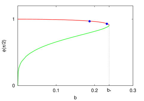
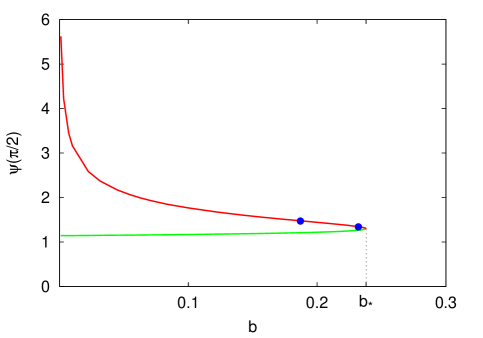
Figure 1: The stable (green) and the unstable (red) axially symmetric solutions of (46), (represented by their equatorial values), and the bifurcation points of the secondary branches for the sample period $T=5\pi$ (blue).

As to obtaining the diagram on the left one first shows that, near a pole ($\theta=0$) there is a 1-parameter family of analytic solutions of the form $\phi(\theta)=d+d(1-d^{4})\theta^{2}/16+O(\theta^{4})$. One then “shoots” (numerically) such a local solution towards the equator and adjusts the parameter $d$ such that $\partial\phi/\partial\theta$ vanishes at the equator ($\pi/2$). This gives a stable branch emanating from $\phi\equiv 0$ (green in the online version), and an unstable branch (red) emanating from $\phi\equiv 1$ in consistency with Thm. 2 and Proposition 4. Moreover, numerics shows that the lowest eigenvalue $\varsigma$ of the linearisation ((45) with $A\equiv 0$) decreases monotonically from $0$ to $\varsigma=-\Lambda$ (cf. point 3. of Proposition 1) along the unstable branch. An analogous discussion in terms of $\psi$, which makes use of Proposition 3, yields the diagram on the right.

However, the “principal” branches displayed above cannot comprise all solutions - we recall from Sect.3.3.1. that even in the special case $b=0$ there is the symmetry-breaking Kottler family of data. We therefore now look for solutions of the form $\phi(\alpha,\theta)$, i.e. we still assume axial symmetry. For small $b$ one can in fact infer, via an implicit function-argument, the existence of unstable “secondary” branches emanating from each Kottler solution. To see where these branches end up, we rewrite an arbitrary eigenvalue $\lambda$ of the linearised operator (45) at some solution $\phi(\theta)$ on the unstable principal branch in terms of the eigenvalue $\lambda_{\theta}$ of the truncated operator ((45) for $A\equiv 0$). With a corresponding separation of variables in the eigenfunction $\mu=\mu(\alpha,\theta)=\mu_{\alpha}(\alpha)\mu_{\theta}(\theta)$ we find

$$\frac{\lambda}{\Lambda}=\left(\frac{2\pi}{T}\right)^{2}j^{2}+\frac{\lambda_{\theta}}{\Lambda}\qquad j=0,1,2...$$ (47)

Bifurcation theory (in essence the arguments of Proposition 2) now shows that symmetry breaking can only occur at solutions where the linearised operator has a zero mode. Setting now $\lambda=0$ and using the numerical observation that $\lambda_{\theta}$ changes monotonically from $0$ at $b=b_{*}$ to some negative value (depending on $T$) at $b=0$ we find that (47) has in fact $k$ solutions $j=1,2,....k$ when $T\in(2\pi k,2\pi(k+1)]$ (Fig.1. shows the bifurcation points corresponding to $j=1$ and $j=2$ in the case $T=5\pi$). Further numerical calculations (which are interesting on their own and will be described in detail separately [5]) now in fact reveal that from the bifurcation point labelled $j$ ($1\leq j\leq k$) on the unstable principal branch, there emanates a secondary branch of solutions of the form $\phi_{j}(\alpha,\theta)$ which continues till $b=0$ and terminates at the Kottler solution with precisely $j$ pairs of horizons (cosmological and black hole).

We remark that we cannot rule out the existence of non-axially symmetric solutions. In particular, Thm. 3.1. of [10] has no obvious extension to the present case. However, the existence of such solutions is unlikely as we do not find corresponding bifurcation points on any of the known branches.

We summarize the above exposition in the following Conjecture. The status of point 3. is “truly conjectural” in the sense just mentioned, while points 1. and 2. are “facts”. However, we wish to reserve the term “theorem” to a forthcoming publication [5] where we hope to present a complete analytic proof of existence of the solutions, but in any case a detailed numerical analysis.

Conjecture 1.

The smooth, positive solutions of the Lichnerowicz equation (44) have the following properties:

1. There exists $b_{*}$ ($b_{*}\approx 0.238$) such that for $b\in(0,b_{*})$ there is precisely one stable solution and one unstable solution which only depend on $\theta$ and are equatorially symmetric (the stable and the unstable principal branch). Moreover, for $b=b_{*}$, there is a unique marginally stable solution with the same symmetries, while for $b>b_{*}$ there is no solution. In the limit $b\rightarrow 0$, the stable solutions tend to zero like $b^{1/4}$.

2. If $T\in(2\pi k,2\pi(k+1)]$, there exist $k$ values $b_{1}$…$b_{k}$, with $b_{*}>b_{1}>b_{2}>...>b_{k}>0$ such that, from each point on the unstable principal branch corresponding to $b_{j}$, there bifurcates a branch of unstable solutions depending only on $\alpha$ and $\theta$ (secondary branches). Each such branch continues till $b=0$, where its end point represents the Kottler solution with $j$ pairs of horizons.

3. All solutions are axially symmetric (i.e. independent of $\varphi$)

We finally note that the maximal value $b_{*}\approx 0.238$ obtained from numerics (cf. Fig. 1.), corresponding to $\Lambda|J|\approx 0.159$, significantly exceeds the existence limit given in Thm. 3.1., while it comes remarkably close to the non-existence limit, Thm. 3.2..

3.4 Kerr-de Sitter

The Kerr-de Sitter (KdS) 4-metric reads,

$$\widetilde{d}s_{4}^{2}=\widetilde{g}_{\mu\nu}^{K}dx^{\mu}x^{\nu}=-\frac{\sigma}{\rho^{2}}\left(dt-\frac{a\sin^{2}\theta}{\kappa}d\varphi\right)^{2}+\frac{\rho^{2}}{\sigma}dr^{2}+\frac{\rho^{2}}{\chi}d\theta^{2}+\frac{\chi\sin^{2}\theta}{\rho^{2}}\left(adt-\frac{r^{2}+a^{2}}{\kappa}d\varphi\right)^{2}$$ (48)

in terms of “Boyer-Lindquist”-coordinates with constants $m$, $a$, and $\kappa=1+\Lambda a^{2}/3$, and in terms of the functions

$$\sigma=(r^{2}+a^{2})(1-\frac{\Lambda r^{2}}{3})-2mr,\qquad\rho^{2}=r^{2}+a^{2}\cos^{2}\theta,\qquad\chi=1+\frac{\Lambda a^{2}\cos^{2}\theta}{3}$$ (49)

where $\sigma$ generalises the synonymous function in 3.3.1.

The constants $m$ and $a$ satisfy bounds given by the extreme solutions, but also “absolute” bounds in terms of $\Lambda$ alone, cf. [1, 7, 8, 17] for a discussion.

The twist scalar of (48) as defined after Equ (29) takes the form

$$\widetilde{\omega}_{K}=-2J_{K}\left(\cos^{3}\theta-3\cos\theta-\frac{a^{2}\cos\theta\sin^{4}\theta}{\rho^{2}}\right)$$ (50)

where

$$J_{K}=\frac{ma}{\kappa^{2}}$$ (51)

is the angular momentum as defined in Sect. 3.1. The bounds on $m$ and $a$ entail a bound on $J_{K}$, again in terms of the angular momenta $J_{E}$ of the 1-parameter family of the extreme solutions; the latter satisfy the absolute bound $\Lambda J_{E}\leq\Lambda J_{max}\approx 0.170$ saturated for one particular extreme solution. Interestingly, this value exceeds the non-existence bound of Thm. 3.2. (valid for TPSM solutions of (44) on the round hypertorus (34)).

We now recall how (48) arises from $(t,\varphi)$-symmetric data. The slice $t=const$ is maximal with induced metric

$$ds^{2}_{K}=g_{ij}^{K}dx^{i}dx^{j}=\rho^{2}\left(\frac{dr^{2}}{\sigma}+\frac{d\theta^{2}}{\chi}\right)+\frac{\sin^{2}\theta}{\kappa^{2}\rho^{2}}\left[\chi\left(r^{2}+a^{2}\right)^{2}-\sigma a^{2}\sin^{2}\theta\right]d\varphi^{2}.$$ (52)

This metric still fits on a 3-manifold ${\cal M}$ of topology $\mathbb{S}^{2}\times\mathbb{S}$ [12] which can be seen as in the Kottler case. As before we restrict ourselves to the region $r\in[r_{b},r_{c}]$ where $\sigma\geq 0$, which is bounded by the black hole- and the cosmological horizon. At $\sigma=0$ the metric (52) is regularised by replacing $r$ by $\alpha$ defined via (36) but with $\sigma$ from (49). Thus the metric becomes periodic in $\alpha$ with period

$$P(\Lambda,m,a):=2\int_{r_{b}}^{r_{c}}\sigma^{-\frac{1}{2}}dr.$$ (53)

As we are not interested in the complete set of solutions here, we take $P$ equal to the circumference $T$ of ${\cal M}$ which leaves us with just one pair of horizons.

From Proposition 5, and using Remark 2. after this Proposition, we can now determine the second fundamental form $K_{ij}^{K}$ via $\omega_{K}=\widetilde{\omega}_{K}|_{\cal M}$

With these preparations we now construct new data as follows.

Definition 5.

We set out from non-extreme KdS data $({\cal M},g_{ij}^{K},K_{ij}^{K})$ as SM with angular momentum $J_{K}$ and with $K_{ij}^{K}$ generated via (32) from $\omega_{K}$. For some $J\in\mathbb{R}$ we define $\omega(J)=J\omega_{K}/J_{K}$ and $K_{ij}(J)$ again via (32).

It follows that $K_{ij}(J)=K_{ij}^{K}J/J_{K}$ and $\Omega^{2}(J)=K_{ij}(J)K^{ij}(J)=J^{2}\Omega_{K}^{2}/J_{K}^{2}$. Note that (51) does not hold for $J\neq J_{K}$.

Applying Premoselli’s theorem (Thm. 2) and Propositions 1, 3 and 4 now yields

Theorem 4.

In the setting described in Definition 5. we claim

1. There exists $J_{*}\geq J_{K}$ such that, for $J\in(0,J_{*})$, Equ. (2) with $\Omega(J)$ has at least two positive solutions, one of which is minimal and stable. Moreover, for $J=J_{*}$ there is a unique marginally stable solution, for $J$ slightly below $J_{*}$ there are precisely two solutions, and for $J>J_{*}$ there is no solution. In the limit $J\rightarrow 0$, the family of minimal, stable solutions tends to zero like $(\Lambda J)^{1/4}$.

2. If

   $$\int_{\cal M}\Omega_{K}^{2}dv<\Lambda.V_{K}$$ (54)

   for KdS data with $J_{K}$, $\Omega_{K}$ and volume $V_{K}$, it follows that $J_{*}>J_{K}$.

3. Inequality (54) (and therefore the conclusion of point 2.) always holds for sufficiently small $J_{K}$.

Proof.

We first note that $K_{ij}(J)$ is smooth for all $J\in\mathbb{R}$. Point 1. follows now trivially from the results stated before the theorem and makes no direct reference to the properties of KdS. We have stated this point explicitly to illustrate how Thm. 2 allows to deduce the existence of a large family of solutions from a single one. Regarding the case $J=0$ we note that, apart from $\phi\equiv 0$, non-trivial solutions definitely exist as well, namely solutions to the Yamabe problem [27]; however, we have no information about their multiplicity and propagation to $J\neq 0$ here. To prove 2. we conclude indirectly: Assume that $J_{*}=J_{K}$ which means that, within the 1-parameter family of $K_{ij}(J)$-tensors generated from $\omega(J)$ with $J\in\mathbb{R}$ as in Definition 5, the KdS tensor $K_{ij}^{K}$ had in fact the maximal angular momentum permitted by Premoselli’s theorem. Then 2. of that theorem would imply that the KdS data are marginally stable. However, (54) together with Proposition 1 implies strict instability, a contradiction. (Note that this Proposition applies here directly since KdS are ID rather than just a SM).

For the final point 3. it suffices to show that $\Omega_{K}^{2}<\Lambda$ for small $J_{K}$. This is intuitively clear as $\Omega_{K}^{2}$ is of order $J_{K}^{2}$ near $J_{K}=0$. To see this in detail, it is useful to rescale all variables and constants to the dimensionless quantities

$$\bar{r}=\sqrt{\Lambda}r\qquad\bar{\theta}=\theta\qquad\bar{\varphi}=\varphi,\qquad\bar{a}=\sqrt{\Lambda}a\qquad\bar{m}=\sqrt{\Lambda}m\qquad\bar{J}_{K}=\Lambda J_{K}$$ (55)

In terms of these variables, the KdS metric and the terms characterising rotation take the forms

$$ds^{2}_{K}=\Lambda^{-1}\bar{d}s^{2}_{K}\qquad\omega_{K}=\Lambda^{-1}\bar{\omega}_{K}\qquad\Omega_{K}^{2}=\Lambda\bar{\Omega}_{K}^{2}$$ (56)

where all quantities on the l.h.s. are functions of $\Lambda,m,a,r$ and $\theta$, while all quantities with bars can be written in terms of the functions $\bar{r},\bar{\theta}$ and constants $\bar{m}$ and $\bar{a}$ only (and hence do not depend explicitly on $\Lambda$).

Using (33) we now observe that $\bar{\Omega}_{K}$ can be written as $\bar{\Omega}_{K}(\bar{r},\bar{\theta},\bar{m},\bar{a})=\bar{J}_{K}\bar{\Omega}_{K,0}(\bar{r},\bar{\theta},\bar{m},\bar{a})$. We first show that $\bar{\Omega}_{K,0}^{2}$ is analytic in all arguments. This follows from the fact the denominator in (33) only vanishes on the axis where, however, it is “regularized” by the zeros of the numerator in the same manner as in the Bowen-York example, and we still have $\bar{\Omega}_{K}^{2}=f\sin^{2}\bar{\theta}$ near the axis with an analytic function $f$. Next we recall that, for regular KdS data, $\bar{m}$ and $|\bar{a}|$ are bounded from above (by a certain number). Therefore, $\bar{\Omega}_{K,0}^{2}(\bar{r},\bar{\theta},\bar{m},\bar{a})$, being an analytic function on a compact domain, is bounded from above (by a number). This implies that $\bar{\Omega}_{K}=\bar{J}_{K}\bar{\Omega}_{K,0}$ can be made as small as needed by decreasing $\bar{J}_{K}$.

We conclude that the KdS metric can indeed be “overspun” in the sense that, for small $J_{K}$, one can put more angular momentum than (51) on the background (52). (We remark that our notion of “overspinning” has nothing to do with attempts of exceeding the angular momentum limit of extreme Kerr black holes, cf. [11]). ∎

We finish with two remarks.

“Conformally relaxed” Kerr-de Sitter data.

Premoselli’s theorem and the previous one imply that for any KdS seed data with $J_{K}$ small enough, there exist stable, minimal data which are conformal to these KdS data. We call them “conformally relaxed”, (while the unstable KdS data themselves are “conformally excited”). In view of their stability, they will necessarily (by Proposition 2) inherit the axisymmetry of the KdS seed, and they will have the same angular momentum by virtue of the conformal invariance of (25). These data will very likely be non-stationary - in any case, again due to their stability, they cannot be a member of the KdS family with different parameters, as follows from the proof of the above theorem. In case the data are really dynamic, it would be interesting to determine their time evolution. Due to axisymmetry, this evolution would preserve the angular momentum. Therefore, it is not impossible that the resulting spacetime settles down to the same member of the KdS family one started with.

Data with marginally outer trapped surfaces.

Within the conformal method, there has been considered the problem of finding ID which contain (marginally) outer trapped surfaces ((M)OTS). This was accomplished by imposing suitable boundary conditions on the SM, first in the asymptotically flat context [14, 28], but recently also for compact manifolds with boundary [22, 23]. However, this work does not cover the Lichnerowicz equation with the present sign of the coefficient of $\phi^{5}$. It would be interesting to handle this case as well [34]. This seems to require combining the techniques of the aforementioned papers with those of Hebey et al. [19] and/or Premoselli [31].

In the examples considered in this paper, both the Kottler as well as the KdS family of data contain minimal surfaces. In the former case, the minimal surfaces are expected to turn into MOTS when a small angular momentum is added. In the same manner, MOTS should arise when the angular momentum of KdS is slightly reduced or increased beyond the stationary value as described above. It would be interesting to settle this in the generic case.

Acknowledgements. We are grateful to Patryk Mach for verifying numerically point 3 in Conjecture 1, and to Lars Andersson, Robert Beig, Piotr Chruściel, Emmanuel Hebey, Patryk Mach and Bruno Premoselli for helpful discussions and correspondence. The research of P.B., and a visit of W.S. to Cracow, were supported by the Polish National Science Centre grant no. DEC-2012/06/A/ST2/00397. The research of W.S. was funded by the Austrian Science Fund (FWF): P23337-N16

References

- [1] Akcay S and Matzner R 2011 The Kerr-de Sitter universe Class. Quantum Grav. 28 085012
- [2] Andersson L, Mars M and Simon W 2008 Stability of marginally outer trapped surfaces and existence of marginally outer trapped tubes Adv. Theor. Math. Phys. 12 853
- [3] Bardeen J M 1970 A variational principle for rotating stars in General Relativity Astrophys. J. 162 71
- [4] Beig R 2000 Generalised Bowen-York initial data in Cotsakis S and Gibbons G W (Eds.) Mathematical and Quantum Aspects of Relativity and Cosmology Lecture Notes in Physics 537 55
- [5] Bizoń P Mach P and Simon W in preparation
- [6] Bowen J M and York J 1980 Time-asymmetric initial data for black holes and black-hole collisions Phys. Rev. D 21 2047
- [7] Caldarelli M M, Cognola G and Klemm D 2000 Thermodynamics of Kerr-Newman-AdS Black Holes and Conformal Field Theories Class. Quantum Grav. 17 399
- [8] Cho J-H, Ko Y and Nam S 2010 The entropy function for the extremal Kerr-(anti-)de Sitter black holes Ann. Phys. NY 325 1517
- [9] Chouikha R 1967 Curvature properties and singularities of certain constant scalar curvature metrics unpublished
- [10] Chruściel P T and Gicquaud R 2015 Bifurcating solutions of the Lichnerowicz equation arXiv:1506.00101; Ann. Henri Poincaré to be published.
- [11] Colleoni M, Barack L 2015 Overspinning a Kerr black hole: the effect of self-force Phys Rev. D 91 104024
- [12] Cortier J 2013 Gluing construction of initial data with Kerr-de Sitter ends Ann. Henri Poincaré 14 1109
- [13] Crandall M G and Rabinowitz P H 1973 Bifurcation, perturbation of simple eigenvalues, and linearized stability Arch. Ration. Mech. and Anal. 52 161
- [14] Dain S 2004 Trapped surfaces as boundaries for the constraint equations Class.Quant.Grav. 21 555-574; 2005 Class. Quantum Grav. 22 769
- [15] Dain S 2006 A variational principle for stationary, axisymmetric solutions of Einstein’s equations Class. Quantum Grav. 23 6857
- [16] Dain S, Lousto C and Takahashi R 2002 New conformally flat initial data for spinning black holes Phys. Rev. D 65 104038
- [17] Gabach Clement M E, Reiris M and Simon W 2015 The area-angular momentum inequality for black holes in cosmological spacetimes Class. Quantum Grav. 32 (2015) 145006
- [18] Hebey E 2008 Existence, stability and instability for Einstein-scalar field Lichnerowicz equations. IAS lectures unpublished http://www3.u-cergy.fr/hebey.
- [19] Hebey E, Pacard F and Pollack D 2008 A variational analysis of Einstein-scalar field Lichnerowicz equations on compact Riemanian manifolds Commun. Math. Phys. 278 117
- [20] Hebey E and Veronelli G 2013 The Lichnerowicz equation in the closed case of the Einstein-Maxwell theory Trans. Am. Math. Soc. 366 1179
- [21] Hebey E and Vaugon M 1991 Multiplicité pour le probléme de Yamabe C. R. Acad. Sci. Paris t.312 Série I 237
- [22] Holst M and Meier C 2014 Non-CMC Solutions to the Einstein Constraint Equations on Asymptotically Euclidean Manifolds with Apparent Horizon Boundaries Class. Quantum Grav. 32 025006
- [23] Holst M and Tsogtgerel G 2013 The Lichnerowicz equation on compact manifolds with boundary Class. Quantum Grav. 30 205011
- [24] Isenberg J 2014 Initial value problem in General Relativity The Springer Handbook of Spacetime eds A Ashtekar and V Petkov (New York:Springer) http://arxiv.org/abs/1304.1960
- [25] Isenberg J 1995 Constant mean curvature solutions of the Einstein constraint equations on closed manifolds Class. Quantum Grav. 12 2249
- [26] Jin Q, Li Y and Xu H 2008 Symmetry and asymmetry: the method of moving spheres Adv. Diff. Equ. 13 7-8 601
- [27] Lee J M and Parker T H 1987 The Yamabe Problem Bull. Am. Math. Soc. (New Ser.) 17 1 37
- [28] Maxwell D 2004 Solutions of the Einstein Constraint Equations with Apparent Horizon Boundaries Commun. Math. Phys. 253 561
- [29] Nariai H 1951 On a new cosmological solution of Einstein’s field equations of gravitation Sci. Rep. I (Tokohu Univ.) Ser. 1 35 62
- [30] Pletka S 2015 Master thesis, University of Vienna http://othes.univie.ac.at
- [31] Premoselli B 2015 Effective multiplicity for the Einstein-scalar field Lichnerowicz equation Calc. Var. 53 29
- [32] Schoen R 1989 Variational theory for the Total Scalar Curvature Functional for Riemannian metrics and related topics Topics in calculus of variations ed M Giaquinta Lecture Notes in Math 1365 (New York: Springer) p 120
- [33] Stanciulescu C 1998 Spherically symmetric solutions of the vacuum Einstein field equations with positive cosmological constant Diploma Thesis DissD.3438 University of Vienna
- [34] Tsogtgerel G 2015 On the Lichnerowicz equation and the prescribed scalar-mean curvature problem in the compact-with-boundary setting talk given at Focus Program on 100 Years of General Relativity, Fields Institute, Toronto