PeakSegJoint: fast supervised peak detection via joint segmentation of multiple count data samples

Abstract

Joint peak detection is a central problem when comparing samples in genomic data analysis, but current algorithms for this task are unsupervised and limited to at most 2 sample types. We propose PeakSegJoint, a new constrained maximum likelihood segmentation model for any number of sample types. To select the number of peaks in the segmentation, we propose a supervised penalty learning model. To infer the parameters of these two models, we propose to use a discrete optimization heuristic for the segmentation, and convex optimization for the penalty learning. In comparisons with state-of-the-art peak detection algorithms, PeakSegJoint achieves similar accuracy, faster speeds, and a more interpretable model with overlapping peaks that occur in exactly the same positions across all samples.

1 Introduction: Joint supervised peak detection in ChIP-seq data

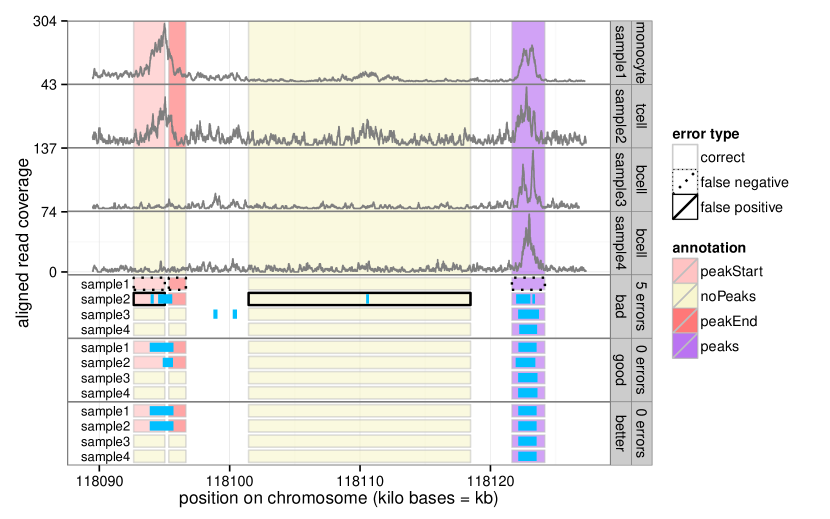
Figure 1: Labeled ChIP-seq coverage data for $S=4$ samples (top 4 panels) with 3 peak models (bottom 3 panels). An ideal peak model minimizes the number of incorrect labels (false positives are too many peaks and false negatives are not enough peaks). The “good” model achieves 0 errors but the “better” model is more interpretable since overlapping peaks in different samples always occur in the exact same positions.

Chromatin immunoprecipitation sequencing (ChIP-seq) is an experimental technique used for genome-wide profiling of histone modifications and transcription factor binding sites (Bailey et al., 2013). Each experiment yields a set of sequence reads which are aligned to a reference genome, and then the number of aligned reads are counted at each genomic position. To compare samples at a given genomic position, biologists visually examine coverage plots such as Figure 1 for presence or absence of common “peaks.” In machine learning terms, a single sample over $B$ base positions is a vector of non-negative count data $\mathbf{z}\in\mathbb{Z}_{+}^{B}$ and a peak detector is a binary classifier $c:\mathbb{Z}_{+}^{B}\rightarrow\{0,1\}^{B}$. The positive class is peaks and the negative class is background noise. Importantly, peaks and background occur in long contiguous segments across the genome.

In this paper we use the supervised learning framework of Hocking et al. (2014), who proposed to use labels obtained from manual visual inspection of genome plots. For each labeled genomic region $i\in\{1,\dots,n\}$ there is a set of count data $\mathbf{z}_{i}$ and labels $L_{i}$ (“noPeaks,” “peaks,” etc. as in Figure 1). These labels define a non-convex annotation error function

$$E[c(\mathbf{z}_{i}),L_{i}]=\text{FP}[c(\mathbf{z}_{i}),L_{i}]+\text{FN}[c(\mathbf{z}_{i}),L_{i}]$$ (1)

which counts the number of false positive (FP) and false negative (FN) regions, so it takes values in the non-negative integers. In this framework the goal of learning is to find a peak detection algorithm $c$ that minimizes the number of incorrect labels (1) on a test set of data:

$$\operatorname*{minimize}_{c}\sum_{i\in\text{test}}E[c(\mathbf{z}_{i}),L_{i}].$$ (2)

In practical situations we have $S>1$ samples, and a matrix $\mathbf{Z}\in\mathbb{Z}_{+}^{B\times S}$ of count data. For example in Figure 1 we have $S=4$ samples. In these data we are not only interested in accurate peak detection in individual samples, but also in detecting the differences between samples. In particular, an ideal model of a multi-sample data set is a joint peak detector with identical overlapping peak positions across samples (the “better” model in Figure 1).

1.1 Contributions and organization

The main contribution of this paper is the PeakSegJoint model for supervised joint peak detection. Unlike previous methods (Section 2), it is the first joint peak detector that explicitly models any number of sample types (Section 3). A secondary contribution is the JointZoom heuristic segmentation algorithm, and a supervised learning algorithm for efficiently selecting the PeakSegJoint model complexity (Section 4). We show test error and timing results in Section 5, provide a discussion in Section 6, and propose some future research directions in Section 7.

2 Related work

2.1 Single-sample ChIP-seq peak detectors

There are many different unsupervised peak detection algorithms (Wilibanks and Facciotti, 2010; Rye et al., 2010; Szalkowski and Schmid, 2011), and the current state-of-the-art is the supervised PeakSeg model of Hocking et al. (2015).

In the multi-sample setting of this paper, each of these algorithms may be applied independently to each sample. The drawback of these methods is that the peaks do not occur in the same positions across each sample, so it is not straightforward to determine differences between samples.

2.2 Methods for several data sets

This paper is concerned with the particular setting of analyzing several samples (perhaps of different cell types) of the same experiment type. For example, Figure 1 shows 2 bcell samples, 1 monocyte sample, and 1 tcell sample (all of the H3K4me3 experiment type). As far as we know, there are no existing algorithms that can explicitly model these data.

The most similar peak detectors in the bioinformatics literature model several samples of the same cell type. For example, the JAMM algorithm of Ibrahim et al. (2014) can analyze several samples, but is limited to a single cell type since it assumes that each sample is a replicate with the exact same peak pattern. So to analyze the data of Figure 1 one would have to run JAMM 3 times (once for each cell type), and the resulting peaks would not be the same across cell types. Another example is the PePr algorithm of Zhang et al. (2014), which can model either one or two cell types, but is unsuitable for analysis of three or more cell types. In contrast, PeakSegJoint is for data from several samples without limit on the number of cell types.

Although not the subject of this paper, there are several algorithms designed for the analysis of data from several different ChIP-seq experiments (Ernst and Kellis, 2012; Hoffman et al., 2012; Zeng et al., 2013). In these models, the input is one sample (e.g. monocyte cells) with different experiments such as H3K4me3 and H3K36me3. Also, Choi et al. (2009) proposed a model for one sample with both ChIP-seq and ChIP-chip data. In contrast, PeakSegJoint takes as input several samples (e.g. monocyte, tcell, bcell) for one experiment such as H3K4me3.

3 Models

We begin by summarizing the single-sample PeakSeg model, and then introduce the multi-sample PeakSegJoint model.

3.1 PeakSeg: finding the most likely $0,\dots,p_{\text{max}}$ peaks in a single sample

This section describes the PeakSeg model of Hocking et al. (2015), which is the current state-of-the-art peak detection algorithm in the McGill benchmark data set of Hocking et al. (2014).

Given a single sample profile $\mathbf{z}\in\mathbb{Z}_{+}^{B}$ of aligned read counts on $B$ bases, and a maximum number of peaks $p_{\text{max}}$, the PeakSeg model for the mean vector $\mathbf{m}\in\mathbb{R}^{B}$ with $p\in\{0,\dots,p_{\text{max}}\}$ peaks is

$$\mathbf{\tilde{m}}^{p}(\mathbf{z})=\operatorname*{arg\,min}_{\mathbf{m}\in\mathbb{R}^{B}} \ \ \text{PoissonLoss}(\mathbf{m},\mathbf{z})$$ (PeakSeg)

such that $$\ \ \operatorname*{Peaks}(\mathbf{m})=p,$$ (3)

$$\forall j\in\{1,\dots,B\}, \ \ P_{j}(\mathbf{m})\in\{0,1\},$$ (4)

where the Poisson loss function is

$$\text{PoissonLoss}(\mathbf{m},\mathbf{z})=\sum_{j=1}^{B}m_{j}-z_{j}\log m_{j}.$$ (5)

Note that the optimization objective of minimizing the Poisson loss is equivalent to maximizing the Poisson likelihood. The model complexity (3) is the number of peaks

$$\operatorname*{Peaks}(\mathbf{m})=(\operatorname*{Segments}(\mathbf{m})-1)/2,$$ (6)

which is a function of the number of piecewise constant segments

$$\operatorname*{Segments}(\mathbf{m})=1+\sum_{j=2}^{B}I(m_{j}\neq m_{j-1}).$$ (7)

Finally, the peak indicator at base $j$ is defined as the cumulative sum of signs of changes

$$P_{j}(\mathbf{m})=\sum_{k=2}^{j}\operatorname{sign}(m_{k}-m_{k-1}),$$ (8)

with $P_{1}(\mathbf{m})=0$ by convention. The constraint (4) means that the peak indicator $P_{j}(\mathbf{m})\in\{0,1\}$ can be used to classify each base $j\in\{1,\dots B\}$ as either background noise $P_{j}(\mathbf{m})=0$ or a peak $P_{j}(\mathbf{m})=1$. In other words, $\mathbf{\tilde{m}}^{p}(\mathbf{z})$ is a piecewise constant vector that changes up, down, up, down (and not up, up, down). Thus the even numbered segments are interpreted as peaks, and the odd numbered segments are interpreted as background noise.

Note that since PeakSeg is defined for a single sample, it may be independently applied to each sample in data sets such as Figure 1. However, any overlapping peaks in different samples will not necessarily occur in the same positions. In the next section we fix this problem by proposing the more interpretable multi-sample PeakSegJoint model.

3.2 PeakSegJoint: finding the most likely common peak in $0,\dots,S$ samples

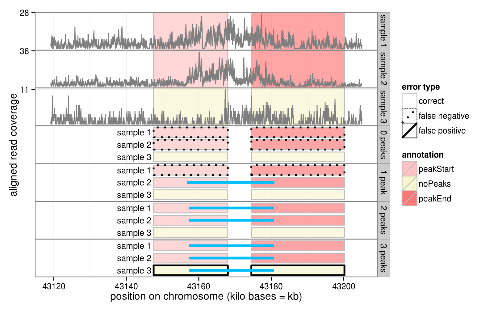
Figure 2: A labeled data set with $S=3$ samples (top 3 panels) and the PeakSegJoint models for $p\in\{0,1,2,3\}$ peaks (bottom 4 panels).

For $S$ sample profiles $\mathbf{z}_{1},\dots,\mathbf{z}_{S}\in\mathbb{Z}_{+}^{B}$ defined on the same $B$ bases, we stack the vectors into a matrix $\mathbf{Z}\in\mathbb{Z}_{+}^{B\times S}$ of count data. Consider the following model for the mean matrix $\mathbf{M}\in\mathbb{R}^{B\times S}$ which allows each sample to have either 0 or 1 peaks, with a total of $p\in\{0,\dots,S\}$ peaks:

$$\mathbf{\hat{M}}^{p}(\mathbf{Z})=\operatorname*{arg\,min}_{\mathbf{M}\in\mathbb{R}^{B\times S}} \ \ \sum_{s=1}^{S}\text{PoissonLoss}(\mathbf{m}_{s},\mathbf{z}_{s})$$ (PeakSegJoint)

such that $$\ \forall s\in\{1,\dots,S\},\,\operatorname*{Peaks}(\mathbf{m}_{s})\in\{0,1\},$$ (9)

$$\ \forall s\in\{1,\dots,S\},\,\forall j\in\{1,\dots,B\},\,P_{j}(\mathbf{m}_{s})\in\{0,1\},$$ (10)

$$\ p=\sum_{s=1}^{S}\operatorname*{Peaks}(\mathbf{m}_{s})$$ (11)

$$\ \forall s_{1}\neq s_{2}\mid\operatorname*{Peaks}(\mathbf{m}_{s_{1}})=\operatorname*{Peaks}(\mathbf{m}_{s_{2}})=1,\,\forall j\in\{1,\dots,B\},$$

$$\ \ P_{j}(\mathbf{m}_{s_{1}})=P_{j}(\mathbf{m}_{s_{2}}).$$ (12)

The first two constraints are similar to the PeakSeg model constraints. The constraint on the number of peaks per sample (9) means that each sample may have either zero or one peak. The constraint (10) requires the segment mean $\mathbf{m}_{s}$ of each sample to have alternating changes (up, down, up, down and not up, up, down). The overall constraint (11) means that there is a total of $p$ samples with exactly 1 peak. The last constraint (12) means that peaks should occur in the exact same positions in each sample. The PeakSegJoint model for a data set with $S=3$ samples is shown in Figure 2.

3.3 Supervised penalty learning

In the last section we considered data $\mathbf{Z}\in\mathbb{Z}_{+}^{B\times S}$ for $S$ samples in a single genomic region with $B$ bases. Now assume that we have data $\mathbf{Z}_{1},\dots,\mathbf{Z}_{n}\in\mathbb{Z}_{+}^{B\times S}$ for $n$ genomic regions, along with annotated region labels $L_{1},\dots,L_{n}$.

For each genomic region $i\in\{1,\dots,n\}$ we can compute a sequence of PeakSegJoint models $\mathbf{\hat{M}}^{0}(\mathbf{Z}_{i}),\dots,\mathbf{\hat{M}}^{S}(\mathbf{Z}_{i})$, but how will we predict which of these $S+1$ models will be best? This is the segmentation model selection problem, which we propose to solve via supervised learning of a penalty function.

First, for a positive penalty constant $\lambda\in\mathbb{R}_{+}$, we define the optimal number of peaks as

$$p^{*}(\lambda,\mathbf{Z})=\operatorname*{arg\,min}_{p\in\{0,\dots,S\}}p\lambda+\text{PoissonLoss}\left[\mathbf{\hat{M}}^{p}(\mathbf{Z}),\mathbf{Z}\right].$$ (13)

Also suppose that we can compute $d$-dimensional sample-specific feature vectors $\mathbf{x}\in\mathbb{R}^{d}$ and stack them to obtain feature matrices $\mathbf{X}_{1},\dots,\mathbf{X}_{n}\in\mathbb{R}^{d\times S}$. We will learn a function $f:\mathbb{R}^{d\times S}\rightarrow\mathbb{R}$ that predicts region-specific penalty values $f(\mathbf{X}_{i})=\log\lambda_{i}\in\mathbb{R}$ for each genomic region $i$. In particular we will learn a weight vector $\mathbf{w}\in\mathbb{R}^{d}$ in a linear function $f_{\mathbf{w}}(\mathbf{X})=\mathbf{w}^{\intercal}\mathbf{X}\mathbf{1}_{S}$, where $\mathbf{1}_{S}$ is a vector of $S$ ones.

For supervision we use the annotated region labels $L_{i}$ to compute the number of incorrect regions (1) for each model size $p$, and then a target interval $\mathbf{y}_{i}=(\underline{y}_{i},\overline{y}_{i})$ of penalty values (Rigaill et al., 2013). Briefly, a predicted penalty in the target interval $f(\mathbf{X}_{i})\in\mathbf{y}_{i}$ implies that the PeakSegJoint model with $p^{*}\left[\exp f(\mathbf{X}_{i}),\mathbf{Z}_{i}\right]$ peaks achieves the minimum number of incorrect labels $L_{i}$, among all $S+1$ PeakSegJoint models for genomic region $i$.

A target interval $\mathbf{y}$ is used with the squared hinge loss $\phi(x)=(x-1)^{2}I(x\leq 1)$ to define the surrogate loss

$$\ell\left[\mathbf{y},\,\log\hat{\lambda}\right]=\phi\big{[}\log\hat{\lambda}-\underline{y}\big{]}+\phi\big{[}\overline{y}-\log\hat{\lambda}\big{]},$$ (14)

for a predicted penalty value $\hat{\lambda}\in\mathbb{R}_{+}$. For a weight parameter $\mathbf{w}\in\mathbb{R}^{d}$, the convex average surrogate loss is

$$\mathcal{L}(\mathbf{w})=\frac{1}{n}\sum_{i=1}^{n}\ell\left[\mathbf{y}_{i},\,f_{\mathbf{w}}(\mathbf{X}_{i})\right].$$ (15)

Finally, we add a 1-norm penalty to regularize and encourage a sparse weight vector, thus obtaining the following convex supervised penalty learning problem:

$$\mathbf{\hat{w}}^{\gamma}=\operatorname*{arg\,min}_{\mathbf{w}\in\mathbb{R}^{d}}\mathcal{L}(\mathbf{w})+\gamma||\mathbf{w}||_{1}.$$ (16)

To predict on test data $\mathbf{Z}$ with features $\mathbf{X}$, we compute the predicted penalty $\hat{\lambda}=\exp f_{\mathbf{\hat{w}}}(\mathbf{X})$, the predicted number of peaks $\hat{p}=p^{*}(\hat{\lambda},\mathbf{Z})$, and finally the predicted mean matrix $\mathbf{\hat{M}}^{\hat{p}}(\mathbf{Z})$. Each column/sample of the mean matrix has either two changes (the second segment is the peak) or no changes (no peak).

4 Algorithms

4.1 Heuristic discrete optimization for joint segmentation

The PeakSegJoint model is defined as the solution to an optimization problem with a convex objective function and non-convex constraints. Real data sets $\mathbf{Z}\in\mathbb{Z}_{+}^{B\times S}$ may have a very large number of data points to segment $B$. Explicitly computing the maximum likelihood and feasibility for all $O(B^{2})$ possible peak start/endpoints is guaranteed to find the global optimum, but would take too much time. Instead, we propose to find an approximate solution using a new discrete optimization algorithm called JointZoom (Algorithm 1).

The main idea of the JointZoom algorithm is to first zoom out (downsample the data) repeatedly by a factor of $\beta$, obtaining a new data matrix of size $b\times S$, where $b\ll B$ (line 1). Then we solve the PeakSegJoint problem for $p$ peaks via GridSearch (line 2), a sub-routine that checks all $O(b^{2})$ possible peak start and end positions. Then we zoom in by a factor of $\beta$ (line 4) and refine the peak positions in $O(\beta^{2})$ time via SearchNearPeak (line 5). After having zoomed back in to the BinSize=1 level we return the final Peak positions, and the $p$ Samples in which that peak was observed.

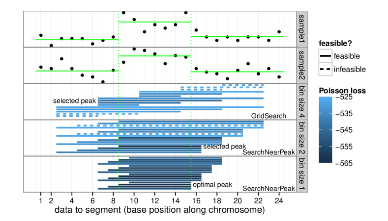
Figure 3: Demonstration of the JointZoom segmentation algorithm. For a data set with $B=24$ data points and $S=2$ samples (top 2 panels), the algorithm with zoom factor of $\beta=2$ proceeds as follows. First, the Poisson loss and feasibility (10) is computed via GridSearch over all peak starts and ends at bin size 4. The feasible model with minimum Poisson loss is selected, the bin size is decreased to 2, and SearchNearPeak considers a new set of models around the selected peak starts and ends. We continue and return the optimal model at bin size 1 (shown in green). Interactive figure at %****␣HOCKING-PeakSegJoint-paper.tex␣Line␣575␣****http://bit.ly/1AA6TgK

0:  count data $\mathbf{Z}\in\mathbb{Z}_{+}^{B\times S}$, number of peaks $p\in\{0,\dots,S\}$, zoom factor $\beta\in\{2,3,\dots\}$.

1:  $\textrm{BinSize}\leftarrow\textsc{MaxBinSize}(B,\beta)$.

2:  $\textrm{Peak},\textrm{Samples}\leftarrow\textsc{GridSearch}(\mathbf{Z},p,\textrm{BinSize})$.

3:  while $1<\textrm{BinSize}$ do

4:     $\textrm{BinSize}\leftarrow\textrm{BinSize}/\beta$.

5:     $\textrm{Peak}\leftarrow\textsc{SearchNearPeak}(\mathbf{Z},\textrm{Samples},\textrm{BinSize},\textrm{Peak})$

6:  end while

7:  return  Peak, Samples.

Algorithm 1 JointZoom, available at https://github.com/tdhock/PeakSegJoint

For example if we fix the zoom factor at $\beta=2$, a demonstration of the algorithm on a small data set with $B=24$ points is shown in Figure 3. MaxBinSize returns 4, so GridSearch considers 15 models of $b=7$ data points at bin size 4, and then SearchNearPeak considers 16 models each at bin sizes 2 and 1. In the real data set of Figure 2, there are $B=85846$ data points, MaxBinSize returns 16384, GridSearch considers 10 models of $b=6$ data points, and then SearchNearPeak considers 16 models each at bin sizes 8192, 4096, …, 4, 2, 1.

Overall JointZoom with zoom factor $\beta$ searches a total of $O(\beta^{2}\log B)$ models, and computing the likelihood and feasibility for each model is an $O(pB)$ operation, so the algorithm has a time complexity of $O(\beta^{2}pB\log B)$. Thus for a count data matrix $\mathbf{Z}\in\mathbb{Z}_{+}^{B\times S}$, computing the sequence of PeakSegJoint models $\mathbf{\hat{M}}^{0}(\mathbf{Z}),\dots,\mathbf{\hat{M}}^{S}(\mathbf{Z})$ takes $O(\beta^{2}SB\log B)$ time.

Finally note that when there is only $S=1$ sample, JointZoom can be used to find an approximate solution to the PeakSeg model with $p=1$ peak.

4.2 Convex optimization for supervised penalty learning

The convex supervised learning problem (16) can be solved using gradient-based methods such as FISTA, a Fast Iterative Shinkage-Thresholding Algorithm (Beck and Teboulle, 2009). For FISTA with constant step size we also need a Lipschitz constant of $\mathcal{L}(\mathbf{w})$. Following the arguments of Flamary et al. (2012), we derived a Lipschitz constant of $\sum_{i=1}^{n}||\mathbf{X}_{i}||_{F}^{2}/n$. Finally, we used the subdifferential stopping criterion of Rigaill et al. (2013).

5 Results

5.1 Accuracy of PeakSegJoint on benchmark data sets

We used McGill benchmark data sets from http://cbio.ensmp.fr/~thocking/chip-seq-chunk-db/ which included a total of 12,826 manually annotated region labels (Hocking et al., 2014). Each data set contains labels grouped into windows of nearby regions (from 4 to 30 windows per data set). For each data set, we performed 6 random splits of windows into half train, half test. Since there are multiple peaks per window, and PeakSegJoint can detect at most 1 peak per sample, we divided each window into separate PeakSegJoint problems of size $B$ (a hyper-parameter tuned via grid search).

We compared the test error of PeakSegJoint with three single-sample models (Figure 4). In all 7 of the McGill benchmark data sets, our proposed PeakSegJoint model achieved test error rates comparable to the previous state-of-the-art PeakSeg model. In contrast, the baseline hmcan.broad (Ashoor et al., 2013) and macs (Zhang et al., 2008) models from the bioinformatics literature were each only effective for a single experiment type (either H3K36me3 or H3K4me3, but not both).

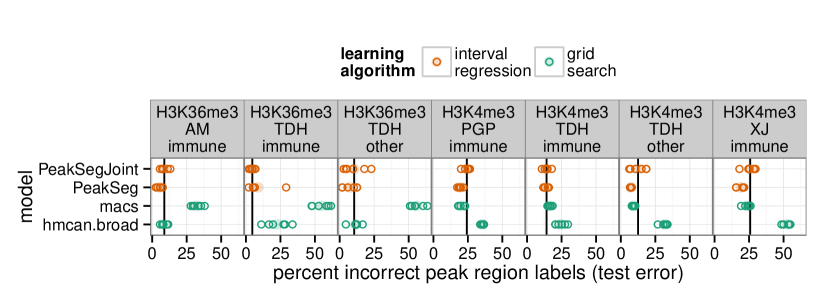
Figure 4: Test error of peak detectors in the 7 McGill benchmark data sets (panels from left to right). Each dot shows one of 6 train/test splits, and the black vertical line marks the mean of the PeakSegJoint model.

5.2 Speed of heuristic PeakSegJoint algorithm

The JointZoom algorithm is orders of magnitude faster than existing Poisson segmentation algorithms (Figure 5). For simulated single-sample, single-peak data sets of size $B\in\{10^{1},\dots,10^{6}\}$, we compared JointZoom with the $O(B\log B)$ unconstrained pruned dynamic programming algorithm (pDPA) of Cleynen et al. (2014) (R package Segmentor3IsBack), and the $O(B^{2})$ constrained dynamic programming algorithm (cDPA) of Hocking et al. (2015) (R package PeakSegDP). We set the maximum number of segments to 3 in the pDPA and cDPA, meaning one peak. Figure 5 indicates that the JointZoom algorithm of PeakSegJoint enjoys the same $O(B\log B)$ asymptotic behavior as the pDPA. However the JointZoom algorithm is faster than both the cDPA and pDPA by at least two orders of magnitude for the range of data sizes that is typical for real data ($10^{2}<B<10^{6}$).

These speed differences are magnified when applying these Poisson segmentation models to real ChIP-seq data sets. For example, the hg19 human genome assembly has about $3\times 10^{9}$ bases. For the H3K36me3_AM_immune data set, a resolution of about 200 kilobases per problem was optimal, so running PeakSegJoint on the entire human genome means solving about 15,000 segmentation problems. PeakSegJoint takes about 0.1 seconds to solve each of those problems (Figure 5), meaning a total computation time of about 25 minutes. In contrast, using the pDPA or cDPA would be orders of magnitude slower (hours or days of computation).

Figure 5: Timings of three Poisson segmentation algorithms on simulated data sets of varying size $B$. The grey shaded area represents the range of problem sizes selected in the McGill benchmark data sets.

6 Discussion

The table below presents a summary of our proposed PeakSegJoint model alongside several other peak detection algorithms. Time complexity is for detecting one peak in $B$ data points. The “?” of the unsupervised joint peak detectors means that their articles did not discuss time complexity (Zhang et al., 2008; Ashoor et al., 2013; Ibrahim et al., 2014; Zhang et al., 2014).

Algorithm	Samples	Cell types	Time complexity	Learning
macs	1	1	?	unsupervised
hmcan.broad	1	1	?	unsupervised
PeakSeg (cDPA)	1	1	$O(B^{2})$	supervised
JAMM	$\geq 1$	1	?	unsupervised
PePr	$\geq 2$	1–2	?	unsupervised
PeakSegJoint (JointZoom)	$\geq 1$	$\geq 1$	$O(B\log B)$	supervised

6.1 Multi-sample PeakSegJoint versus single-sample PeakSeg

The PeakSegJoint model is explicitly designed for supervised, multi-sample peak detection problems such as the McGill benchmark data sets that we considered. We observed that the single-sample PeakSeg model is as accurate as PeakSegJoint in these data (Figure 4). However, any single-sample model is qualitatively inferior to a multi-sample model since it can not predict overlapping peaks at the exact same positions. Furthermore, the $O(B\log B)$ JointZoom algorithm can compute the PeakSegJoint model much faster than the $O(B^{2})$ cDPA of PeakSeg (Figure 5).

6.2 PeakSegJoint versus other joint peak detectors

We attempted to compare with the multi-sample JAMM and PePr algorithms. The PeakSegJoint model is more interpretable than these existing methods, since it is able to handle several sample types. This was advantageous in data sets such as Figure 1, which contains 3 cell types: tcell, bcell, and monocyte. The PeakSegJoint model can be run once on all cell types, and the resulting model can be easily interpreted to find the differences, since peaks occur in the exact same locations across samples. In contrast, existing methods such as JAMM or PePr are less suitable to analyze this data set since they are limited to modeling only 1 or 2 cell types. We nevertheless downloaded and ran the algorithms separately on each sample type, but both JAMM and PePr produced errors and so were unable to analyze the McGill benchmark data sets.

7 Conclusions

We proposed the PeakSegJoint model for supervised joint peak detection. It generalizes the state-of-the-art PeakSeg model to multiple samples. We proposed the JointZoom Poisson segmentation algorithm that is orders of magnitude faster than existing algorithms. Finally, we showed that choosing the number of peaks in PeakSegJoint using supervised penalty learning yields test error rates that are comparable to the previous state-of-the-art PeakSeg model.

For future work, we would be interested in a theoretical analysis analogous to the work of Cleynen and Lebarbier (2014), which could suggest the form of the optimal penalty function to choose the number of peaks in the PeakSegJoint model.

References

- Ashoor et al. [2013] H. Ashoor, A. Hérault, A. Kamoun, F. Radvanyi, V. B. Bajic, E. Barillot, and V. Boeva. HMCan: a method for detecting chromatin modifications in cancer samples using ChIP-seq data. Bioinformatics, 29(23):2979–2986, 2013.
- Bailey et al. [2013] T. Bailey, P. Krajewski, I. Ladunga, C. Lefebvre, Q. Li, T. Liu, P. Madrigal, C. Taslim, and J. Zhang. Practical guidelines for the comprehensive analysis of ChIP-seq data. PLoS computational biology, 9(11):e1003326, 2013.
- Beck and Teboulle [2009] A. Beck and M. Teboulle. A fast iterative shrinkage-thresholding algorithm for linear inverse problems. SIAM J. Imaging Sciences, 2(1):183–202, 2009.
- Choi et al. [2009] H. Choi, A. Nesvizhskii, D. Ghosh, and Z. Qin. Hierarchical hidden Markov model with application to joint analysis of ChIP-chip and ChIP-seq data. Bioinformatics, 25:1715–1721, 2009.
- Cleynen et al. [2014] A. Cleynen, M. Koskas, E. Lebarbier, G. Rigaill, and S. Robin. Segmentor3IsBack: an R package for the fast and exact segmentation of Seq-data. Algorithms for Molecular Biology, 9:6, 2014.
- Ernst and Kellis [2012] J. Ernst and M. Kellis. ChromHMM: automating chromatin-state discovery and characterization. Nature Methods, 9(3):215–216, 2012.
- Flamary et al. [2012] R. Flamary, N. Jrad, R. Phlypo, M. Congedo, and A. Rakotomamonjy. Mixed-norm regularization for brain decoding. HAL tech. report 00708243, 2012.
- Hocking et al. [2014] T. D. Hocking, P. Goerner-Potvin, A. Morin, X. Shao, and G. Bourque. Visual annotations and a supervised learning approach for evaluating and calibrating ChIP-seq peak detectors. arXiv:1409.6209, 2014.
- Hocking et al. [2015] T. D. Hocking, G. Rigaill, and G. Bourque. PeakSeg: constrained optimal segmentation and supervised penalty learning for peak detection in count data. In Proc. 32nd ICML, 2015.
- Hoffman et al. [2012] M. M. Hoffman, O. J. Buske, J. Wang, Z. Weng, J. A. Bilmes, and W. S. Noble. Unsupervised pattern discovery in human chromatin structure through genomic segmentation. Nature Methods, 9:473–476, 2012. doi: 10.1038/nmeth.1937.
- Ibrahim et al. [2014] M. M. Ibrahim, S. A. Lacadie, and U. Ohler. JAMM: a peak finder for joint analysis of NGS replicates. Bioinformatics, page btu568, 2014.
- Cleynen and Lebarbier [2014] A. Cleynen and E. Lebarbier. Segmentation of the Poisson and negative binomial rate models: a penalized estimator. ESAIM: PS, 18:750–769, 2014.
- Rigaill et al. [2013] G. Rigaill, T. Hocking, J.-P. Vert, and F. Bach. Learning sparse penalties for change-point detection using max margin interval regression. In Proc. 30th ICML, pages 172–180, 2013.
- Rye et al. [2010] M. B. Rye, P. Sætrom, and F. Drabløs. A manually curated ChIP-seq benchmark demonstrates room for improvement in current peak-finder programs. Nucleic acids research, 2010.
- Szalkowski and Schmid [2011] A. M. Szalkowski and C. D. Schmid. Rapid innovation in ChIP-seq peak-calling algorithms is outdistancing benchmarking efforts. Briefings in Bioinformatics, 12(6):626–633, 2011.
- Wilibanks and Facciotti [2010] E. Wilibanks and M. Facciotti. Evaluation of Algorithm Performance in ChIP-Seq Peak Detection. PLoS ONE, 5(7), 2010.
- Zeng et al. [2013] X. Zeng, R. Sanalkumar, E. Bresnick, H. Li, Q. Chang, and S. Keles. jMOSAiCS: joint analysis of multiple ChIP-seq datasets. Genome Biology, 14(4):R38, 2013. ISSN 1465-6906.
- Zhang et al. [2008] Y. Zhang, T. Liu, C. A. Meyer, J. Eeckhoute, D. S. Johnson, B. E. Bernstein, C. Nusbaum, R. M. Myers, M. Brown, W. Li, et al. Model-based analysis of ChIP-Seq (MACS). Genome Biol, 9(9):R137, 2008.
- Zhang et al. [2014] Y. Zhang, Y.-H. Lin, T. D. Johnson, L. S. Rozek, and M. A. Sartor. PePr: a peak-calling prioritization pipeline to identify consistent or differential peaks from replicated ChIP-Seq data. Bioinformatics, 30(18):2568–2575, 2014.