A Dynamic Structure for High Dimensional Covariance Matrices and its Application in Portfolio Allocation

Abstract

Estimation of high dimensional covariance matrices is an interesting and important research topic. In this paper, we propose a dynamic structure and develop an estimation procedure for high dimensional covariance matrices. Asymptotic properties are derived to justify the estimation procedure and simulation studies are conducted to demonstrate its performance when the sample size is finite. By exploring a financial application, an empirical study shows that portfolio allocation based on dynamic high dimensional covariance matrices can significantly outperform the market from 1995 to 2014. Our proposed method also outperforms portfolio allocation based on the sample covariance matrix and the portfolio allocation proposed in Fan, Fan and Lv (2008).

KEY WORDS: Dynamic structure, factor models, high dimensional covariance matrices, iterative algorithm, kernel smoothing, portfolio allocation, single-index models.

SHORT TITLE: Dynamic Structure for HDCM.

1 Introduction

Covariance matrix estimation is an important topic in statistics and econometrics with wide applications in many disciplines, such as economics, finance and psychology. A traditional approach to estimating covariance matrices is based on the sample covariance matrix. However, the sample covariance matrix would not be a good choice when the dimension is large, and especially when the inverse is required, which is often the case when constructing a portfolio allocation in finance. This is because the estimation errors would accumulate when using the inverse of the sample covariance matrix to estimate the inverse of the covariance matrix. When the size of the covariance matrix is large, the cumulative estimation error would become unacceptable even if the estimation error of each entry of the covariance matrix is tiny.

In recent years there has been various attempts to address high dimensional covariance matrix estimation. Usually, a sparsity condition is imposed to control the trade-off between variance and bias. See, Wu and Pourahmadi (2003), El Karoui (2008), Bickel and Levina (2008a, 2008b), Lam and Fan (2009), Fan, Liao, and Mincheva (2011), and the references therein. Fan, Fan and Lv (2008) considered a different approach by imposing a factor model and estimated the covariance matrix based on this structure.

Most of the literature addressing high dimensional covariance matrix estimation assumes that the covariance matrix is constant over time. However, in many applications, covariance matrices are dynamic. For example, today’s optimal portfolio allocation may not be optimal tomorrow, or next month. Therefore, when applying the formula for Markowitz’s optimal portfolio allocation (Markowitz 1959), the covariance matrix used should be dynamic and allowed to change over time.

In order to introduce a dynamic structure for covariance matrices, one cannot simply assume each entry of a covariance matrix is a function of time because this would not serve very well in prediction. Instead, we start with an approach stimulated by Fan, Fan and Lv (2008) which is based on the Fama-French three-factor model (Fama and French, 1992, 1993)

$$y_{t}=\alpha+X_{t}^{\!\mbox{\scriptsize T}}\mbox{\bf a}+\epsilon_{t},$$ (1.1)

where $y_{t}$ is the excess return of an asset and $X_{t}$ is the vector of the three factors at time $t$. To make (1.1) more flexible, we allow a to depend on the values of the three factors at time $t-1$. To avoid the so-called ‘curse of dimensionality’, we assume this dependence is through a linear combination of the values of the three factors at time $t-1$, which brings us to

$$y_{t}=\alpha(X_{t-1}^{\!\mbox{\scriptsize T}}\mbox{\boldmath{$\beta$}})+X_{t}^{\!\mbox{\scriptsize T}}\mbox{\bf a}(X_{t-1}^{\!\mbox{\scriptsize T}}\mbox{\boldmath{$\beta$}})+\epsilon_{t}.$$ (1.2)

This motivates a dynamic structure for the covariance matrix of a random vector $Y_{t}$ through an adaptive varying coefficient model which we shall now introduce.

Suppose $(X_{t}^{\!\mbox{\scriptsize T}},\ Y_{t}^{\!\mbox{\scriptsize T}})$, $t=1,\ \cdots,\ n$, is a time series, where $Y_{t}$ is a $p_{n}$ dimensional vector and $X_{t}$ is a $q$ dimensional factor. An underlying assumption throughout this paper is that $p_{n}\longrightarrow\infty$ when $n\longrightarrow\infty$, and $q$ is fixed. Also, we assume that $X_{t}$, $t=1,\ \cdots,\ n$, is a stationary Markov process. We assume

$$Y_{t}=\mbox{\bf g}(X_{t-1}^{\!\mbox{\scriptsize T}}\mbox{\boldmath{$\beta$}})+\mbox{\boldmath{$\Phi$}}(X_{t-1}^{\!\mbox{\scriptsize T}}\mbox{\boldmath{$\beta$}})X_{t}+\mbox{\boldmath{$\epsilon$}}_{t},\quad\|\mbox{\boldmath{$\beta$}}\|=1,\quad\beta_{1}>0$$ (1.3)

where $\mbox{\boldmath{$\beta$}}=(\beta_{1},\ \cdots,\ \beta_{q})^{\!\mbox{\scriptsize T}}$, $\mbox{\boldmath{$\Phi$}}(X_{t-1}^{\!\mbox{\scriptsize T}}\mbox{\boldmath{$\beta$}})$ is a factor loading matrix which is varying over $X_{t-1}^{\!\mbox{\scriptsize T}}\mbox{\boldmath{$\beta$}}$, and $\{\mbox{\boldmath{$\epsilon$}}_{t}$, $t=1,\ \cdots,\ n\}$ are random errors which are independent of $\{X_{t}$, $t=1,\ \cdots,\ n\}$. We assume

$$E(\mbox{\boldmath{$\epsilon$}}_{t}|\{\mbox{\boldmath{$\epsilon$}}_{l}:\ l<t\})=\mbox{\bf 0},\quad\mbox{cov}(\mbox{\boldmath{$\epsilon$}}_{t}|\{\mbox{\boldmath{$\epsilon$}}_{l}:\ l<t\})=\boldsymbol{\Sigma}_{0,t}=\mbox{diag}\left(\sigma_{1t}^{2},\ \cdots,\ \sigma_{p_{n}t}^{2}\right)$$

where

$$\sigma_{kt}^{2}=\alpha_{k,0}+\sum\limits_{i=1}^{m}\alpha_{k,i}\epsilon_{k,t-i}^{2}+\sum\limits_{j=1}^{s}\gamma_{k,j}\sigma_{k,t-j}^{2},\quad t=2,\ \cdots,\ n,$$ (1.4)

for each $k=1,\ \cdots,\ p_{n}$ and for some integers $m$ and $s$. Let ${\cal F}_{t}$ be the $\sigma-$algebra generated by $\{(X_{l}^{\!\mbox{\scriptsize T}},\ \mbox{\boldmath{$\epsilon$}}_{l}^{\!\mbox{\scriptsize T}}):\ l\leq t\}$. The main focus of this paper is on the conditional covariance matrix

$$\mbox{cov}(Y_{t}|{\cal F}_{t-1})=\mbox{\boldmath{$\Phi$}}(X_{t-1}^{\!\mbox{\scriptsize T}}\mbox{\boldmath{$\beta$}})\boldsymbol{\Sigma}_{x}(X_{t-1})\mbox{\boldmath{$\Phi$}}(X_{t-1}^{\!\mbox{\scriptsize T}}\mbox{\boldmath{$\beta$}})^{\!\mbox{\scriptsize T}}+\boldsymbol{\Sigma}_{0,t}$$ (1.5)

where $\boldsymbol{\Sigma}_{x}(X_{t-1})=\mbox{cov}(X_{t}|X_{t-1}).$ In (1.5), $\mbox{\boldmath{$\Phi$}}(\cdot)$, $\beta$, $\boldsymbol{\Sigma}_{x}(\cdot)$, $\alpha_{k,i}$ and $\gamma_{k,j}$, $i=0,\ \cdots,\ m$, $j=1,\ \cdots,\ s$, are unknown and need to be estimated. Not only does (1.5) introduce a dynamic structure for $\mbox{cov}(Y_{t}|{\cal F}_{t-1})$, but also reduces the number of unknown parameters from $p_{n}(p_{n}+1)/2$ to $p_{n}q+q^{2}$ unknown functions and $q+s+m+1$ unknown parameters.

We remark that model (1.3) is interesting in its own right, since it combines single-index modelling (Carroll et al., 1997, Härdle et al., 1993, Yu and Ruppert, 2002, Xia and Härdle, 2006, Kong and Xia, 2014) and varying coefficient modelling (Fan and Zhang, 1999, 2000, Fan et al., 2003, Sun et al., 2007, Zhang et al., 2009, Li and Zhang, 2011, Sun et al., 2014). In this paper, as a by-product, an estimation procedure for (1.3) is proposed and an iterative algorithm is developed for implementation purposes.

This paper is organised as follows. We begin in Section 2 with a description of the proposed estimation procedure for $\mbox{cov}(Y_{t}|{\cal F}_{t-1})$. A discussion on bandwidth selection is given in Section 3. In Section 4 we provide asymptotic properties of the estimation procedure. An iterative algorithm to implement the estimation procedure is suggested in Section 5. Using the proposed dynamic structure for covariance matrices and the developed estimation procedure, we outline a process for constructing a portfolio allocation based on the formula for Markowitz’s optimal portfolio in Section 6. The performance of the estimation procedure and portfolio allocation are also assessed by simulation studies in Section 7. In Section 8, we apply the portfolio allocation methodology to a data set consisting of 49 industry portfolios which are freely available from Kenneth French’s website. We find that the proposed methodology works surprisingly well. All the detailed proofs are relegated to the appendix.

2 Estimation procedure

In this section, we are going to introduce an estimation procedure for $\mbox{cov}(Y_{t}|{\cal F}_{t-1})$. We will first estimate $\beta$, $\mbox{\boldmath{$\Phi$}}(\cdot)$, $\boldsymbol{\Sigma}_{x}(\cdot)$, $\alpha_{k,i}$ and $\gamma_{k,j}$, and denote the resulting estimators by $\hat{\mbox{\boldmath{$\beta$}}}$, $\hat{\mbox{\boldmath{$\Phi$}}}(\cdot)$, $\hat{\boldsymbol{\Sigma}}_{x}(\cdot)$, $\hat{\alpha}_{k,i}$ and $\hat{\gamma}_{k,j}$ for $i=0,\ \cdots,\ m$ and $j=1,\ \cdots,\ s$. Let $\hat{\boldsymbol{\Sigma}}_{0,t}$ be $\boldsymbol{\Sigma}_{0,t}$ with $\alpha_{k,i}$ and $\gamma_{k,j}$ being replaced by $\hat{\alpha}_{k,i}$ and $\hat{\gamma}_{k,j}$ respectively. We use

$$\widehat{\mbox{cov}}(Y_{t}|{\cal F}_{t-1})=\hat{\mbox{\boldmath{$\Phi$}}}(X_{t-1}^{\!\mbox{\scriptsize T}}\hat{\mbox{\boldmath{$\beta$}}})\hat{\boldsymbol{\Sigma}}_{x}(X_{t-1})\hat{\mbox{\boldmath{$\Phi$}}}(X_{t-1}^{\!\mbox{\scriptsize T}}\hat{\mbox{\boldmath{$\beta$}}})^{\!\mbox{\scriptsize T}}+\hat{\boldsymbol{\Sigma}}_{0,t}$$ (2.1)

to estimate $\mbox{cov}(Y_{t}|{\cal F}_{t-1})$.

Throughout this paper, for any function $f(x)$, we use $\dot{f}(x)$ to denote its derivative. For any functional matrix $F=(f_{ij}(x))$, we define its derivative as $\dot{F}=(\dot{f}_{ij}(x))$. For any integers $p$ and $q$, we use $\mbox{\bf 0}_{p\times q}$ to denote a $p\times q$ matrix with each entry being $0$, and $\mbox{\bf 1}_{p}$ to denote a $p$-dimensional vector with each component being $1$.

2.1 Estimation of $\beta$

A Taylor expansion gives, for $X_{i}^{\!\mbox{\scriptsize T}}\mbox{\boldmath{$\beta$}}$ in a neighbourhood of $X_{j}^{\!\mbox{\scriptsize T}}\mbox{\boldmath{$\beta$}}$,

$$\mbox{\boldmath{$\Phi$}}(X_{i}^{\!\mbox{\scriptsize T}}\mbox{\boldmath{$\beta$}})\approx\mbox{\boldmath{$\Phi$}}(X_{j}^{\!\mbox{\scriptsize T}}\mbox{\boldmath{$\beta$}})+\dot{\mbox{\boldmath{$\Phi$}}}(X_{j}^{\!\mbox{\scriptsize T}}\mbox{\boldmath{$\beta$}})(X_{i}-X_{j})^{\!\mbox{\scriptsize T}}\mbox{\boldmath{$\beta$}}$$

and

$$\mbox{\bf g}(X_{i}^{\!\mbox{\scriptsize T}}\mbox{\boldmath{$\beta$}})\approx\mbox{\bf g}(X_{j}^{\!\mbox{\scriptsize T}}\mbox{\boldmath{$\beta$}})+\dot{\mbox{\bf g}}(X_{j}^{\!\mbox{\scriptsize T}}\mbox{\boldmath{$\beta$}})(X_{i}-X_{j})^{\!\mbox{\scriptsize T}}\mbox{\boldmath{$\beta$}}$$

for $j=1,\ \cdots,\ n-1$. This, together with the idea of least squares estimation, brings us to the following local discrepancy function

$$L(\mbox{\bf g}_{1},\ \mbox{\boldmath{$\xi$}}_{1},\ A_{1},\ B_{1},\ \cdots,\ \mbox{\bf g}_{n-1},\ \mbox{\boldmath{$\xi$}}_{n-1},\ A_{n-1},\ B_{n-1},\ \mbox{\boldmath{$\beta$}})$$ (2.2)

$$= \sum\limits_{j=1}^{n-1}\sum\limits_{i=2}^{n}\left\|Y_{i}-\mbox{\bf g}_{j}-A_{j}X_{i}-(\mbox{\boldmath{$\xi$}}_{j}+B_{j}X_{i})(X_{i-1}-X_{j})^{\!\mbox{\scriptsize T}}\mbox{\boldmath{$\beta$}}\right\|^{2}K_{h}((X_{i-1}-X_{j})^{\!\mbox{\scriptsize T}}\mbox{\boldmath{$\beta$}}),$$

where: $K_{h}(\cdot)=K(\cdot/h)/h$, $K(\cdot)$ is a kernel function; $h$ is a bandwidth; and $\mbox{\bf g}_{j}$, $\mbox{\boldmath{$\xi$}}_{j}$, $A_{j}$ and $B_{j}$ are used to denote $\mbox{\bf g}(X_{j}^{\!\mbox{\scriptsize T}}\mbox{\boldmath{$\beta$}})$, $\dot{\mbox{\bf g}}(X_{j}^{\!\mbox{\scriptsize T}}\mbox{\boldmath{$\beta$}})$, $\mbox{\boldmath{$\Phi$}}(X_{j}^{\!\mbox{\scriptsize T}}\mbox{\boldmath{$\beta$}})$ and $\dot{\mbox{\boldmath{$\Phi$}}}(X_{j}^{\!\mbox{\scriptsize T}}\mbox{\boldmath{$\beta$}})$ respectively. By minimising

$$L(\mbox{\bf g}_{1},\ \mbox{\boldmath{$\xi$}}_{1},\ A_{1},\ B_{1},\ \cdots,\ \mbox{\bf g}_{n-1},\ \mbox{\boldmath{$\xi$}}_{n-1},\ A_{n-1},\ B_{n-1},\ \mbox{\boldmath{$\beta$}})$$

under the conditions

$$\|\mbox{\boldmath{$\beta$}}\|=1,\quad\beta_{1}>0,$$

we use the corresponding value of $\beta$ as the estimator and denote it by $\hat{\mbox{\boldmath{$\beta$}}}$.

2.2 Estimation of $\mbox{\boldmath{$\Phi$}}(\cdot)$ and $\mbox{\bf g}(\cdot)$

Once an estimate $\hat{\mbox{\boldmath{$\beta$}}}$ has been obtained, the estimators of $\mbox{\boldmath{$\Phi$}}(\cdot)$ and $\mbox{\bf g}(\cdot)$ can be constructed row by row through a standard univariate varying coefficient model for each component of $Y_{t}$. Let

$$\mbox{\bf g}(\cdot)=\left(g_{1}(\cdot),\ \cdots,\ g_{p_{n}}(\cdot)\right)^{\!\mbox{\scriptsize T}},\quad\mbox{\boldmath{$\Phi$}}(\cdot)=\left(\mbox{\bf a}_{1}(\cdot),\ \cdots,\ \mbox{\bf a}_{p_{n}}(\cdot)\right)^{\!\mbox{\scriptsize T}},\quad Y_{t}=(y_{1,t},\ \cdots,\ y_{p_{n},t})^{\!\mbox{\scriptsize T}}.$$

By (1.3), and for $k=1,\ \cdots,\ p_{n}$, we have the following synthetic univariate varying coefficient model

$$y_{k,t}=g_{k}(X_{t-1}^{\!\mbox{\scriptsize T}}\hat{\mbox{\boldmath{$\beta$}}})+X_{t}^{\!\mbox{\scriptsize T}}\mbox{\bf a}_{k}(X_{t-1}^{\!\mbox{\scriptsize T}}\hat{\mbox{\boldmath{$\beta$}}})+\epsilon_{kt},$$

for $t=2,\ \cdots,\ n.$ By local linear estimation for standard varying-coefficient models, and for any given $u$, we have

$$\hat{\mbox{\bf a}}_{k}(u)=(I_{q},\ \mbox{\bf 0}_{q\times(q+2)})\left({\cal X}^{\!\mbox{\scriptsize T}}W{\cal X}\right)^{-1}{\cal X}^{\!\mbox{\scriptsize T}}W\mbox{\bf y}_{k},\quad\hat{g}_{k}(u)=(\mbox{\bf 0}_{1\times q},\ 1,\ \mbox{\bf 0}_{1\times(q+1)})\left({\cal X}^{\!\mbox{\scriptsize T}}W{\cal X}\right)^{-1}{\cal X}^{\!\mbox{\scriptsize T}}W\mbox{\bf y}_{k},$$

where

$$\mbox{\bf y}_{k}=(y_{k,2},\ \cdots,\ y_{k,n})^{\!\mbox{\scriptsize T}},\quad{\cal X}=\left(\begin{array}[]{cccc}X_{2}^{\!\mbox{\scriptsize T}}&1&(X_{1}^{\!\mbox{\scriptsize T}}\hat{\mbox{\boldmath{$\beta$}}}-u)&(X_{1}^{\!\mbox{\scriptsize T}}\hat{\mbox{\boldmath{$\beta$}}}-u)X_{2}^{\!\mbox{\scriptsize T}}\\ \vdots&\vdots&\vdots&\vdots\\ X_{n}^{\!\mbox{\scriptsize T}}&1&(X_{n-1}^{\!\mbox{\scriptsize T}}\hat{\mbox{\boldmath{$\beta$}}}-u)&(X_{n-1}^{\!\mbox{\scriptsize T}}\hat{\mbox{\boldmath{$\beta$}}}-u)X_{n}^{\!\mbox{\scriptsize T}}\end{array}\right),$$

$$W=\mbox{diag}\left(K_{h_{1}}(X_{1}^{\!\mbox{\scriptsize T}}\hat{\mbox{\boldmath{$\beta$}}}-u),\ \cdots,\ K_{h_{1}}(X_{n-1}^{\!\mbox{\scriptsize T}}\hat{\mbox{\boldmath{$\beta$}}}-u)\right),$$

and $h_{1}$ is a bandwidth.

2.3 Estimation of $\boldsymbol{\Sigma}_{x}(\cdot)$

In order to estimate $E(X_{t}|X_{t-1}=\mbox{\bf u})$ and $E(X_{t}X_{t}^{\!\mbox{\scriptsize T}}|X_{t-1}=\mbox{\bf u})$, for any given u, we use the local constant estimators

$$\widehat{E}(X_{t}|X_{t-1}=\mbox{\bf u})=\frac{\sum\limits_{t=2}^{n}X_{t}K_{h_{2}}(\|X_{t-1}-\mbox{\bf u}\|)}{\sum\limits_{t=2}^{n}K_{h_{2}}(\|X_{t-1}-\mbox{\bf u}\|)},$$ (2.3)

$$\widehat{E}(X_{t}X_{t}^{\!\mbox{\scriptsize T}}|X_{t-1}=\mbox{\bf u})=\frac{\sum\limits_{t=2}^{n}X_{t}X_{t}^{\!\mbox{\scriptsize T}}K_{h_{2}}(\|X_{t-1}-\mbox{\bf u}\|)}{\sum\limits_{t=2}^{n}K_{h_{2}}(\|X_{t-1}-\mbox{\bf u}\|)}.$$

This gives us the following estimator of $\boldsymbol{\Sigma}_{x}(\mbox{\bf u})$

$$\hat{\boldsymbol{\Sigma}}_{x}(\mbox{\bf u}) = \widehat{E}(X_{t}X_{t}^{\!\mbox{\scriptsize T}}|X_{t-1}=\mbox{\bf u})-\widehat{E}(X_{t}|X_{t-1}=\mbox{\bf u})\left\{\widehat{E}(X_{t}|X_{t-1}=\mbox{\bf u})\right\}^{\!\mbox{\scriptsize T}}$$ (2.4)

$$= \left\{\mbox{tr}({\cal W})\right\}^{-2}\mbox{\bf X}^{\!\mbox{\scriptsize T}}\left\{\mbox{tr}({\cal W}){\cal W}-{\cal W}\mbox{\bf 1}\mbox{\bf 1}^{\!\mbox{\scriptsize T}}{\cal W}\right\}\mbox{\bf X}$$

where

$$\mbox{\bf X}=(X_{2},\ \cdots,\ X_{n})^{\!\mbox{\scriptsize T}},\quad{\cal W}=\mbox{diag}(K_{h_{2}}(\|X_{1}-\mbox{\bf u}\|),\ \cdots,\ K_{h_{2}}(\|X_{n-1}-\mbox{\bf u}\|)),$$

and $h_{2}$ is a bandwidth.

2.4 Estimation of $\boldsymbol{\Sigma}_{0,t}$

For each $k$, $k=1,\ \cdots,\ p_{n}$, let

$$r_{k,t}=\hat{\epsilon}_{k,t}=y_{k,t}-\hat{g}_{k}(X_{t-1}^{\!\mbox{\scriptsize T}}\hat{\mbox{\boldmath{$\beta$}}})-X_{t}^{\!\mbox{\scriptsize T}}\hat{\mbox{\bf a}}_{k}(X_{t-1}^{\!\mbox{\scriptsize T}}\hat{\mbox{\boldmath{$\beta$}}}).$$

By (1.4), we have the following synthetic GARCH model

$$\sigma_{kt}^{2}=\alpha_{k,0}+\sum\limits_{i=1}^{m}\alpha_{k,i}r_{k,t-i}^{2}+\sum\limits_{j=1}^{s}\gamma_{k,j}\sigma_{k,t-j}^{2},\quad t=2,\ \cdots,\ n$$ (2.5)

which is equivalent to

$$r_{k,t}^{2}=\alpha_{k,0}+\sum\limits_{i=1}^{\max(m,s)}(\alpha_{k,i}+\gamma_{k,i})r_{k,t-i}^{2}+\eta_{kt}-\sum\limits_{j=1}^{s}\gamma_{k,j}\eta_{k,t-j},\quad t=2,\ \cdots,\ n$$

where $\eta_{kt}=r_{k,t}^{2}-\sigma_{kt}^{2}$, $\gamma_{k,i}=0$ when $i>s$, and $\alpha_{k,i}=0$ when $i>m$.

Once $\alpha_{k,i}$ and $\gamma_{k,j}$ have been estimated, by substituting them into (2.5) and setting $\sigma_{kl}^{2}=r_{k,l}^{2}$ for $l\leq\max(m,s)$, we can obtain an estimator $\hat{\sigma}_{kt}^{2}$ of $\sigma_{kt}^{2}$ and hence an estimator $\hat{\boldsymbol{\Sigma}}_{0,t}$ of $\boldsymbol{\Sigma}_{0,t}$.

For each $k$, $k=1,\ \cdots,\ p_{n}$, let $\mbox{\boldmath{$\theta$}}_{k}=(\alpha_{k,0},\ \cdots,\ \alpha_{k,m},\ \gamma_{k,1},\ \cdots,\ \gamma_{k,s})^{\!\mbox{\scriptsize T}}$. We are going to use a quasi-maximum likelihood approach to estimate $\mbox{\boldmath{$\theta$}}_{k}$. We define the negative quasi log-likelihood function of $\mbox{\boldmath{$\theta$}}_{k}$ as

$$Q_{k,n}(\mbox{\boldmath{$\theta$}}_{k})={n^{-1}}\sum_{t=2}^{n}\left\{\frac{r_{k,t}^{2}}{\sigma_{k,t}^{2}(\mbox{\boldmath{$\theta$}}_{k})}+\log\sigma_{k,t}^{2}(\mbox{\boldmath{$\theta$}}_{k})\right\}$$ (2.6)

where $\sigma_{k,t}^{2}(\mbox{\boldmath{$\theta$}}_{k})$ are recursively defined by (2.5) with initial values being either

$$r_{k,0}^{2}=\cdots=r_{k,1-m}^{2}=\sigma_{k,0}^{2}=\cdots=\sigma_{k,1-s}^{2}=\alpha_{k,0}$$

or

$$r_{k,0}^{2}=\cdots=r_{k,1-m}^{2}=\sigma_{k,0}^{2}=\cdots=\sigma_{k,1-s}^{2}=r_{k,0}^{2}.$$

By minimising $Q_{k,n}(\mbox{\boldmath{$\theta$}}_{k})$ with respect to $\mbox{\boldmath{$\theta$}}_{k}$ on a compact set $\Lambda$ defined in (B3) in Appendix A, we use the minimiser $\hat{\mbox{\boldmath{$\theta$}}}_{k}$ to estimate $\mbox{\boldmath{$\theta$}}_{k}$.

3 Bandwidth selection

The choice of the bandwidth $h$, used in the estimation of $\beta$, is not crucial. According to some numerical analysis not presented in this paper for brevity, the accuracy of the estimator $\hat{\mbox{\boldmath{$\beta$}}}$ is not very sensitive to $h$, as long as $h$ is within in a reasonable range. In the computational algorithm for estimating $\beta$, see Section 5, we recommend choosing a bandwidth $h$ equal to around $20\%$ of the following range

$$\max\{X_{1}^{\!\mbox{\scriptsize T}}\tilde{\mbox{\boldmath{$\beta$}}},\cdots,X_{n}^{\!\mbox{\scriptsize T}}\tilde{\mbox{\boldmath{$\beta$}}}\}-\min\{X_{1}^{\!\mbox{\scriptsize T}}\tilde{\mbox{\boldmath{$\beta$}}},\cdots,X_{n}^{\!\mbox{\scriptsize T}}\tilde{\mbox{\boldmath{$\beta$}}}\}$$ (3.1)

where $\tilde{\mbox{\boldmath{$\beta$}}}$ is a randomly chosen initial estimate of $\beta$. We update $h$ on subsequent iterations by replacing $\tilde{\mbox{\boldmath{$\beta$}}}$ in (3.1) with the most recent estimate of $\beta$. This approach is employed in the simulation studies and real data analysis of this paper.

We now focus on the selection of the bandwidth $h_{1}$, used in the estimation of $\mbox{\bf g}(\cdot)$ and $\mbox{\boldmath{$\Phi$}}(\cdot)$. The proposed bandwidth selection is based on a $k$-nearest neighbours bandwidth with $k$ being selected by cross-validation. We define the cross-validation statistic by

$$\mbox{CV}(k)=\sum\limits_{t=n-M}^{n}\left\|Y_{t}-\hat{\mbox{\bf g}}^{(t-1)}(X_{t-1}^{\!\mbox{\scriptsize T}}\hat{\mbox{\boldmath{$\beta$}}})-\hat{\mbox{\boldmath{$\Phi$}}}^{(t-1)}(X_{t-1}^{\!\mbox{\scriptsize T}}\hat{\mbox{\boldmath{$\beta$}}})X_{t}\right\|$$ (3.2)

where $\hat{\mbox{\bf g}}^{(t-1)}(\cdot)$ and $\hat{\mbox{\boldmath{$\Phi$}}}^{(t-1)}(\cdot)$ are the respective estimators of $\mbox{\bf g}(\cdot)$ and $\mbox{\boldmath{$\Phi$}}(\cdot)$ using a $k$-nearest neighbours bandwidth based on $(X_{l}^{\!\mbox{\scriptsize T}},\ Y_{l}^{\!\mbox{\scriptsize T}})$, $l=1,\ \cdots,\ t-1$, and where $M$ is a look-back integer parameter such that $M<n-1$.

Hence, denoting the $k$ that minimises $\mbox{CV}(k)$ by $\hat{k}$, we use a $\hat{k}$-nearest neighbours bandwidth in the estimation of $\mbox{\bf g}(\cdot)$ and $\mbox{\boldmath{$\Phi$}}(\cdot)$. The bandwidth $h_{2}$ in the estimation of $\boldsymbol{\Sigma}_{x}(\cdot)$ or $E(X_{t}|X_{t-1}=\mbox{\bf u})$ can also be selected by cross-validation in a similar way.

4 Asymptotic properties

In this section, we are going to present the asymptotic properties of the proposed estimators. We first introduce the following notation which will be used throughout this paper. For any matrix $\mbox{\bf A}=(a_{ij})_{m\times N}$, we use $\lambda_{\min}(\mbox{\bf A})$ and $\lambda_{\max}(\mbox{\bf A})$ to denote respectively the smallest and largest eigenvalues of A. The trace of A is denoted by $\mbox{tr}(\mbox{\bf A})$, the Frobenius norm of A by $\|\mbox{\bf A}\|_{F}$, and the spectral norm (also called operator norm) and element-wise norm by

$$\|\mbox{\bf A}\|=\sqrt{\lambda_{\max}\left(\mbox{\bf A}^{\!\mbox{\scriptsize T}}\mbox{\bf A}\right)},\quad\|\mbox{\bf A}\|_{\infty}=\underset{\underset{{\scriptscriptstyle 1\leq j\leq N}}{{\scriptscriptstyle 1\leq i\leq m}}}{\mathrm{max}}|a_{ij}|$$

respectively. We also define

$$\mbox{\bf U}_{n}=\frac{1}{np_{n}}\sum_{i=2}^{n}\sum_{k=1}^{p_{n}}f(X_{i}^{\!\mbox{\scriptsize T}}\mbox{\boldmath{$\beta$}})\{X_{i-1}-E(X_{i}|X_{i-1}^{\!\mbox{\scriptsize T}}\mbox{\boldmath{$\beta$}})\}\{\dot{g}_{k}(X_{i-1}^{\!\mbox{\scriptsize T}}\mbox{\boldmath{$\beta$}})+\dot{\mbox{\bf a}}_{k}(X_{i-1}^{\!\mbox{\scriptsize T}}\mbox{\boldmath{$\beta$}})X_{i}\}\epsilon_{k,i}$$

and

$$\mbox{\bf V}_{p}={p_{n}^{-1}}\sum_{k=1}^{p_{n}}E\left(f(X_{1}^{\!\mbox{\scriptsize T}}\mbox{\boldmath{$\beta$}})\{X_{1}-E(X_{2}|X_{1}^{\!\mbox{\scriptsize T}}\mbox{\boldmath{$\beta$}})\}^{\otimes 2}\left\{\dot{g}_{k}(X_{1}^{\!\mbox{\scriptsize T}}\mbox{\boldmath{$\beta$}})+\dot{\mbox{\bf a}}_{k}(X_{1}^{\!\mbox{\scriptsize T}}\mbox{\boldmath{$\beta$}})X_{2}\right\}^{2}\right).$$

Theorem 1. Under assumptions (A1 - A5), (B1 - B4), (C1) and (C3) in Appendix A, there exists $C>0$ and a small $\varepsilon>0$ such that

(I)

$$P\left\{\left\|\widehat{\mbox{\boldmath{$\beta$}}}-\mbox{\boldmath{$\beta$}}-\mbox{\bf V}_{p}^{-1}\mbox{\bf U}_{n}\right\|>C\left(h^{3}+\frac{\log(n)}{nh}\right)\right\}\leq O\left(\frac{1}{n^{1+\varepsilon}}\right);$$

(II)

$$P\left\{\sup_{z\in\mathcal{Z}}\left\|\widehat{\mbox{\bf g}}(z)-\mbox{\bf g}(z)\right\|_{\infty}>C\left(h_{1}^{2}+\sqrt{\frac{\log(n)}{nh_{1}}}\right)\right\}\leq O\left({1\over n^{1+\varepsilon}}\right);$$

(III)

$$P\left\{\sup_{z\in\mathcal{Z}}\left\|\widehat{\mbox{\boldmath{$\Phi$}}}(z)-\mbox{\boldmath{$\Phi$}}(z)\right\|_{\infty}>C\left(h_{1}^{2}+\sqrt{\frac{\log(n)}{nh_{1}}}\right)\right\}\leq O\left({1\over n^{1+\varepsilon}}\right);$$

(IV)

$$P\left\{\sup_{1\leq k\leq p_{n}}\left\|\widehat{\mbox{\boldmath{$\theta$}}}_{k}-\mbox{\boldmath{$\theta$}}_{k}\right\|>C\left(h_{1}^{2}+\sqrt{\frac{\log(n)}{nh_{1}}}\right)\right\}\leq O\left({1\over n^{1+\varepsilon}}\right),$$

where $\mathcal{Z}$ is a compact subset of the range of $X_{t}^{\mathrm{{\scriptstyle T}}}\mbox{\boldmath{$\beta$}}$.

Remark 1. Theorem 1 shows that $\|\widehat{\mbox{\boldmath{$\beta$}}}-\mbox{\boldmath{$\beta$}}\|=o_{P}(n^{-1/2})$ when $p_{n}$ diverges to $\infty$ as $n\to\infty$, provided that $\|\mbox{\bf U}_{n}\|=o_{P}(n^{-1/2})$. It indicates that the index $\beta$ is estimated with a rate faster than the normal rate $n^{-1/2}$, which is the optimal rate if $p_{n}$ is fixed. This is known as a ‘blessing of high dimensionality’.

The main interest of this paper is to estimate $\mbox{cov}(Y_{t}|{\cal F}_{t-1})$. To measure the accuracy of an estimator $\hat{M}$ of a matrix $M$ of size $p_{n}$, we use the entropy loss norm, proposed by James and Stein (1961),

$$\left\|\hat{M}-M\right\|_{\boldsymbol{\Sigma}}=p_{n}^{-1/2}\left\|M^{-1/2}\left\{\hat{M}-M\right\}M^{-1/2}\right\|_{F}.$$

To facilitate our presentation, we focus on the convergence of $\widehat{\mbox{cov}}(Y_{n+1}|\mathcal{F}_{n})-\mbox{cov}(Y_{n+1}|\mathcal{F}_{n})$, after obtaining the data $\big{\{}(X_{1},Y_{1}),\cdots,(X_{n},Y_{n})\big{\}}$.

Theorem 2. Under assumptions (A1 - A5), (B1 - B4) and (C1 - C4) in Appendix A, there exist $C>0$ and $\varepsilon>0$ such that, with probability at least $1-n^{-(1+\varepsilon)}$,

$$\left\|\widehat{\mathrm{cov}}(Y_{n+1}|{\cal F}_{n})-\mathrm{cov}(Y_{n+1}|{\cal F}_{n})\right\|_{\boldsymbol{\Sigma}}^{2}\leq p_{n}C\left\{h_{1}^{8}+\left(\frac{\log n}{nh_{1}}\right)^{2}\right\}+C\left(h_{1}^{4}+\frac{\log n}{nh_{1}}\right)+p_{n}^{-1}C\left(h_{2}^{4}+\frac{\log n}{nh_{2}^{q}}\right).$$

Fan, Fan and Lv (2008) and Fan, Liao and Mincheva (2011) showed an estimator of a covariance matrix based on a certain structure would achieve a higher convergence rate than the sample covariance matrix. Theorem 2 tells us the same story. There are three terms to measure the accuracy of $\widehat{\mbox{cov}}(Y_{n+1}|\mathcal{F}_{n})-\mbox{cov}(Y_{n+1}|\mathcal{F}_{n})$. The first two terms tell us how the nonparametric smoothing steps in estimating $\mbox{\boldmath{$\Phi$}}(\cdot)$ affect the performance of $\widehat{\mbox{cov}}(Y_{n+1}|\mathcal{F}_{n})$, and the third term evaluates the influence of conditional covariance matrix $\boldsymbol{\Sigma}_{x}(X_{n})$. It turns out that even though $q-$dimensional smoothing is required, its effect is small and often negligible if $p_{n}$ is large.

5 Computational algorithm

To implement the proposed estimation procedure for $\mbox{cov}(Y_{t}|{\cal F}_{t-1})$, the hardest part is to compute an estimate of $\beta$, which is equivalent to finding the minimum of

$$L(\mbox{\bf g}_{1},\ \mbox{\boldmath{$\xi$}}_{1},\ A_{1},\ B_{1},\ \cdots,\ \mbox{\bf g}_{n-1},\ \mbox{\boldmath{$\xi$}}_{n-1},\ A_{n-1},\ B_{n-1},\ \mbox{\boldmath{$\beta$}})$$

under the conditions

$$\|\mbox{\boldmath{$\beta$}}\|=1,\quad\beta_{1}>0.$$

We now introduce the proposed iterative algorithm which can be used to do this minimisation. Let

$${\cal Q}(\mbox{\bf g}_{1},\ \mbox{\boldmath{$\xi$}}_{1},\ A_{1},\ B_{1},\ \cdots,\ \mbox{\bf g}_{n-1},\ \mbox{\boldmath{$\xi$}}_{n-1},\ A_{n-1},\ B_{n-1},\ \mbox{\boldmath{$\beta$}},\ \mbox{\bf b})$$

$$= \sum\limits_{j=1}^{n-1}\sum\limits_{i=2}^{n}\left\|Y_{i}-\mbox{\bf g}_{j}-A_{j}X_{i}-(\mbox{\boldmath{$\xi$}}_{j}+B_{j}X_{i})(X_{i-1}-X_{j})^{\!\mbox{\scriptsize T}}\mbox{\boldmath{$\beta$}}\right\|^{2}K_{h}((X_{i-1}-X_{j})^{\!\mbox{\scriptsize T}}\mbox{\bf b}),$$

which is $L(\mbox{\bf g}_{1},\ \mbox{\boldmath{$\xi$}}_{1},\ A_{1},\ B_{1},\ \cdots,\ \mbox{\bf g}_{n-1},\ \mbox{\boldmath{$\xi$}}_{n-1},\ A_{n-1},\ B_{n-1},\ \mbox{\boldmath{$\beta$}})$ with the $\beta$ in the kernel function being replaced by b. First of all, randomly choose an initial estimate for $\beta$, denoted by $\tilde{\mbox{\boldmath{$\beta$}}}$, such that $\|\tilde{\mbox{\boldmath{$\beta$}}}\|=1$ and the first component of $\tilde{\mbox{\boldmath{$\beta$}}}$ is positive. Then, iterate between the following two steps until convergence:

1. If this is the first iteration, let $\mbox{\boldmath{$\beta$}}_{0}=\tilde{\mbox{\boldmath{$\beta$}}}$. Otherwise, set $\mbox{\boldmath{$\beta$}}_{0}$ equal to the $\hat{\mbox{\boldmath{$\beta$}}}$ obtained from Step 2 of the previous iteration. Minimise

   $$L(\mbox{\bf g}_{1},\ \mbox{\boldmath{$\xi$}}_{1},\ A_{1},\ B_{1},\ \cdots,\ \mbox{\bf g}_{n-1},\ \mbox{\boldmath{$\xi$}}_{n-1},\ A_{n-1},\ B_{n-1},\ \mbox{\boldmath{$\beta$}}_{0})$$

   with respect to $\mbox{\bf g}_{1},\ \mbox{\boldmath{$\xi$}}_{1},\ A_{1},\ B_{1},\ \cdots,\ \mbox{\bf g}_{n-1},\ \mbox{\boldmath{$\xi$}}_{n-1},\ A_{n-1}$ and $B_{n-1}$, and denote the minimiser by $\hat{\mbox{\bf g}}_{1}$, $\hat{\mbox{\boldmath{$\xi$}}}_{1}$, $\hat{A}_{1}$, $\hat{B}_{1}$, $\cdots$, $\hat{\mbox{\bf g}}_{n-1}$, $\hat{\mbox{\boldmath{$\xi$}}}_{n-1}$, $\hat{A}_{n-1}$ and $\hat{B}_{n-1}$.

2. Minimise

   $${\cal Q}(\hat{\mbox{\bf g}}_{1},\ \hat{\mbox{\boldmath{$\xi$}}}_{1},\ \hat{A}_{1},\ \hat{B}_{1},\ \cdots,\ \hat{\mbox{\bf g}}_{n-1},\ \hat{\mbox{\boldmath{$\xi$}}}_{n-1},\ \hat{A}_{n-1},\ \hat{B}_{n-1},\ \mbox{\boldmath{$\beta$}},\ \mbox{\boldmath{$\beta$}}_{0})$$

   with respect to $\beta$. Denote the minimiser by $\check{\mbox{\boldmath{$\beta$}}}$, and define $\hat{\mbox{\boldmath{$\beta$}}}=\check{\mbox{\boldmath{$\beta$}}}/\|\check{\mbox{\boldmath{$\beta$}}}\|$ when the first component of $\check{\mbox{\boldmath{$\beta$}}}$ is positive and $\hat{\mbox{\boldmath{$\beta$}}}=-\check{\mbox{\boldmath{$\beta$}}}/\|\check{\mbox{\boldmath{$\beta$}}}\|$ otherwise.

The $\hat{\mbox{\boldmath{$\beta$}}}$ resulting from the convergence is the final estimate of $\beta$.

The proposed iterative algorithm is easy to implement as both minimisers in Step 1 and Step 2 have a closed form. Once an estimate of $\beta$ is obtained, the remaining computation of $\mbox{cov}(Y_{t}|{\cal F}_{t-1})$ becomes straightforward.

6 Portfolio allocation

In this section, we will briefly describe the construction of an estimated optimal portfolio allocation based on the proposed dynamic structure and the associated estimation procedure. Since the formula for optimal portfolio allocation contains $E(Y_{t}|{\cal F}_{t-1})$ we shall introduce its estimator $\widehat{E}(Y_{t}|{\cal F}_{t-1})$ first. By taking conditional expectation of (1.3), we have

$$E(Y_{t}|{\cal F}_{t-1})=\mbox{\bf g}(X_{t-1}^{\!\mbox{\scriptsize T}}\mbox{\boldmath{$\beta$}})+\mbox{\boldmath{$\Phi$}}(X_{t-1}^{\!\mbox{\scriptsize T}}\mbox{\boldmath{$\beta$}})E(X_{t}|X_{t-1}).$$

Therefore, we use

$$\widehat{E}(Y_{t}|{\cal F}_{t-1})=\hat{\mbox{\bf g}}(X_{t-1}^{\!\mbox{\scriptsize T}}\hat{\mbox{\boldmath{$\beta$}}})+\hat{\mbox{\boldmath{$\Phi$}}}(X_{t-1}^{\!\mbox{\scriptsize T}}\hat{\mbox{\boldmath{$\beta$}}})\hat{E}(X_{t}|X_{t-1})$$ (6.1)

to estimate $E(Y_{t}|{\cal F}_{t-1})$ where $\hat{E}(X_{t}|X_{t-1})$ is defined in (2.3).

Our estimated optimal portfolio allocation builds on the mean-variance optimal portfolio by Markowitz (1952, 1959). The allocation vector w of $p_{n}$ risky assets, to be held between times $t-1$ and $t$, is defined as the solution to

$$\underset{{\scriptstyle\mathbf{w}}}{\mathrm{min}}\;\mathbf{w}^{\mathrm{{\scriptstyle T}}}\mathrm{cov}(Y_{t}|\mathcal{F}_{t-1})\mathbf{w}$$

$$\mbox{subject to }\mathbf{w}^{\mathrm{{\scriptstyle T}}}\mathbf{1}_{p_{n}}=1\quad\mbox{and}\quad\mathbf{w}^{\mathrm{{\scriptstyle T}}}E(Y_{t}|\mathcal{F}_{t-1})=\delta$$

where $\delta$ is the target return imposed on the portfolio. The solution $\hat{\mbox{\bf w}}$ is given by

$$\hat{\mbox{\bf w}}=\frac{c_{3}-c_{2}\delta}{c_{1}c_{3}-c_{2}^{2}}\widehat{\mbox{cov}}(Y_{t}|{\cal F}_{t-1})^{-1}\mbox{\bf 1}_{p_{n}}+\frac{c_{1}\delta-c_{2}}{c_{1}c_{3}-c_{2}^{2}}\widehat{\mbox{cov}}(Y_{t}|{\cal F}_{t-1})^{-1}\widehat{E}(Y_{t}|{\cal F}_{t-1}),$$ (6.2)

where

$$c_{1}=\mbox{\bf 1}_{p_{n}}^{\!\mbox{\scriptsize T}}\widehat{\mbox{cov}}(Y_{t}|{\cal F}_{t-1})^{-1}\mbox{\bf 1}_{p_{n}},\quad c_{2}=\mbox{\bf 1}_{p_{n}}^{\!\mbox{\scriptsize T}}\widehat{\mbox{cov}}(Y_{t}|{\cal F}_{t-1})^{-1}\widehat{E}(Y_{t}|{\cal F}_{t-1}),$$

$$c_{3}=\widehat{E}(Y_{t}|{\cal F}_{t-1})^{\!\mbox{\scriptsize T}}\widehat{\mbox{cov}}(Y_{t}|{\cal F}_{t-1})^{-1}\widehat{E}(Y_{t}|{\cal F}_{t-1}).$$

7 Simulation studies

In this section, we are going to use a simulated example to show how well the proposed estimation procedure and portfolio allocation works. We shall use $a_{i,j}(\cdot)$ to denote the entry corresponding to the $i$th row and $j$th column of $\mbox{\boldmath{$\Phi$}}(\cdot)$.

We generate 1000 data sets from model (1.3) together with (1.4). We repeat this using the following combinations of $n$ and $p_{n}$: $\{n=1000,p_{n}=50\}$, $\{n=1000,p_{n}=100\}$, $\{n=2000,p_{n}=50\}$ and $\{n=2000,p_{n}=100\}$. We set

$$q=4,\quad m=1,\quad s=1,\quad\mbox{\boldmath{$\beta$}}=\frac{1}{3}(1,\ 2,\ 0,\ 2)^{\!\mbox{\scriptsize T}}.$$

For $k=1,\ \cdots,\ p_{n}$, we set

$$\alpha_{0,k}=0.5,\quad\alpha_{1,k}=0.1,\quad\beta_{1,k}=0.1,\quad g_{k}(z)=\Xi_{0,k}+3\mbox{exp}(-z^{2}),\quad a_{k,1}(z)=\Xi_{1,k}+0.8z,$$

$$a_{k,2}(z)=\Xi_{2,k},\quad a_{k,3}(z)=\Xi_{3,k}+1.5\mbox{sin}(\pi z),\quad a_{k,4}(z)=\Xi_{4,k},$$

where $\Xi_{j,k}$ are some fixed parameters for $j=0,\ \cdots,\ d$ and $k=1,\ \cdots,\ p_{n}$. In order to define $\Xi_{j,k}$, we simulate them independently from a uniform distribution on $[-1,\ 1]$, and use these same values throughout all simulations. For $t=1,\ \cdots,\ n+1$, we generate $X_{t}$ independently from a uniform distribution on $[-1,1]^{q}$, $Z_{t}$ from $p_{n}$-variate standard normal distribution, and $\mbox{\boldmath{$\epsilon$}}_{t}$ through $\mbox{\boldmath{$\epsilon$}}_{t}=\boldsymbol{\Sigma}_{0,t}^{1/2}Z_{t}$. Once both $X_{t}$ and $\mbox{\boldmath{$\epsilon$}}_{t}$ have been generated, $Y_{t}$ can be generated through (1.3) for $t=1,\ \cdots,\ n+1$.

We will initially pretend that $(X_{n+1}^{\!\mbox{\scriptsize T}},\ Y_{n+1}^{\!\mbox{\scriptsize T}})$ is unknown to us, and this will not be used in the estimation of $\mbox{cov}(Y_{n+1}|{\cal F}_{n})$. The purpose of generating an additional data point $(X_{n+1}^{\!\mbox{\scriptsize T}},\ Y_{n+1}^{\!\mbox{\scriptsize T}})$ is to enable us to calculate the 1-period simple return

$$R(\hat{\mbox{\bf w}})=\hat{\mbox{\bf w}}^{\!\mbox{\scriptsize T}}Y_{n+1}$$ (7.1)

of a portfolio allocation $\hat{\mbox{\bf w}}$ formed at time $n$ based on data $(X_{t}^{\!\mbox{\scriptsize T}},\ Y_{t}^{\!\mbox{\scriptsize T}})$, $t=1,\ \cdots,\ n$. In order to evaluate the performance of an estimator $\hat{M}$ of matrix $M$ we use the following metric

$$\Delta(\hat{M},\ M)=\dfrac{\bigl{\|}\hat{M}-M\bigr{\|}_{F}}{\bigl{\|}M\bigr{\|}_{F}}.$$

We also use the Sharpe ratio

$$\mbox{SR}(\hat{\mbox{\bf w}})=\frac{E\left\{R(\hat{\mbox{\bf w}})\right\}}{\mbox{SD}\left\{R(\hat{\mbox{\bf w}})\right\}}$$

to evaluate the performance of $\hat{\mbox{\bf w}}$, where $\mbox{SD}\left\{R(\hat{\mbox{\bf w}})\right\}$ is the standard deviation of $R(\hat{\mbox{\bf w}}).$ We assume a zero risk-free rate for simplicity.

We first examine how well the estimation procedure works. We estimate $\mbox{cov}(Y_{n+1}|{\cal F}_{n})$, and use $\widehat{\mbox{cov}}(Y_{n+1}|{\cal F}_{n})^{-1}$ to estimate $\mbox{cov}(Y_{n+1}|{\cal F}_{n})^{-1}$. The kernel function in the estimation procedure is taken to be the Epanechnikov kernel $K(u)=0.75(1-u^{2})_{+}$, and the bandwidths are selected by the methodology described in Section 3. The results, presented in Tables 1 and 2, show both $\widehat{\mbox{cov}}(Y_{n+1}|{\cal F}_{n})$ and $\widehat{\mbox{cov}}(Y_{n+1}|{\cal F}_{n})^{-1}$ work very well.

Table 1: Mean and Standard Deviation of $\Delta\left(\widehat{\mathrm{cov}}(Y_{n+1}|{\cal F}_{n}),\ \mathrm{cov}(Y_{n+1}|{\cal F}_{n})\right)$

	$\begin{array}[]{c}n=1000\\ p_{n}=50\end{array}$	$\begin{array}[]{c}n=1000\\ p_{n}=100\end{array}$	$\begin{array}[]{c}n=2000\\ p_{n}=50\end{array}$	$\begin{array}[]{c}n=2000\\ p_{n}=100\end{array}$
$E(D)$	0.183	0.189	0.136	0.141
$\mbox{SD}(D)$	0.046	0.049	0.034	0.035

In this table, $D=\Delta\left(\widehat{\mathrm{cov}}(Y_{n+1}|{\cal F}_{n}),\ \mathrm{cov}(Y_{n+1}|{\cal F}_{n})\right)$, and $\mathrm{SD}(D)$ is the standard deviation of $D$.

Table 2: Mean and Standard Deviation of $\Delta\left(\widehat{\mathrm{cov}}(Y_{n+1}|{\cal F}_{n})^{-1},\ \mathrm{cov}(Y_{n+1}|{\cal F}_{n})^{-1}\right)$

	$\begin{array}[]{c}n=1000\\ p_{n}=50\end{array}$	$\begin{array}[]{c}n=1000\\ p_{n}=100\end{array}$	$\begin{array}[]{c}n=2000\\ p_{n}=50\end{array}$	$\begin{array}[]{c}n=2000\\ p_{n}=100\end{array}$
$E(D_{1})$	0.114	0.105	0.078	0.070
$\mbox{SD}(D_{1})$	0.017	0.013	0.012	0.009

In this table, $D_{1}=\Delta\left(\widehat{\mathrm{cov}}(Y_{n+1}|{\cal F}_{n})^{-1},\ \mathrm{cov}(Y_{n+1}|{\cal F}_{n})^{-1}\right)$, and $\mathrm{SD}(D_{1})$ is the standard deviation of $D_{1}$.

We now examine the performance of the proposed portfolio allocation, using a target return $\delta=1\%$, by computing the return as described in (7.1). In order to see how much gain can be made by making use of the dynamic structure, we make a comparison with portfolio allocations based on Markowitz’s formula but where the covariance matrix is estimated using the sample covariance matrix and also the estimator proposed by Fan, Fan and Lv (2008). The mean, standard deviation and Sharpe ratio of the returns are presented in Table 3. For each situation discussed, we see the Sharpe ratio of the proposed portfolio allocation is much bigger than the other two portfolio allocations. This suggests there is significant gain from making use of the dynamic structure of the covariance matrix.

Table 3: Means, Standard Deviations and Sharpe Ratios

	$\begin{array}[]{c}n=1000\\ p_{n}=50\end{array}$	$\begin{array}[]{c}n=1000\\ p_{n}=100\end{array}$	$\begin{array}[]{c}n=2000\\ p_{n}=50\end{array}$	$\begin{array}[]{c}n=2000\\ p_{n}=100\end{array}$
$E\left\{R(\hat{\mbox{\bf w}})\right\}$	0.99%	1.01%	1.03%	1.03%
$E\left\{R(\hat{\mbox{\bf w}}_{1})\right\}$	0.96%	0.96%	1.02%	1.02%
$E\left\{R(\hat{\mbox{\bf w}}_{2})\right\}$	0.96%	0.96%	1.02%	1.02%
$\mbox{SD}\left\{R(\hat{\mbox{\bf w}})\right\}$	0.40%	0.28%	0.39%	0.27%
$\mbox{SD}\left\{R(\hat{\mbox{\bf w}}_{1})\right\}$	1.02%	1.03%	1.03%	1.02%
$\mbox{SD}\left\{R(\hat{\mbox{\bf w}}_{2})\right\}$	0.99%	0.97%	1.02%	1.00%
$\mbox{SR}(\hat{\mbox{\bf w}})$	2.49	3.57	2.63	3.83
$\mbox{SR}(\hat{\mbox{\bf w}}_{1})$	0.94	0.93	0.99	1.00
$\mbox{SR}(\hat{\mbox{\bf w}}_{2})$	0.97	0.99	1.00	1.02

In this table we denote the proposed portfolio allocation by $\hat{\mbox{\bf w}}$, the portfolio allocation formed by Markowitz’s formula using the sample covariance matrix by $\hat{\mbox{\bf w}}_{1}$, and the portfolio allocation formed by Markowitz’s formula using the estimated covariance matrix from Fan, Fan and Lv (2008) by $\hat{\mbox{\bf w}}_{2}$.

8 Real data analysis

In this section, we are going to apply the dynamic structure for covariance matrices to a real data set. We use the term Face (Factor model with an Adaptive-varying-coefficient-model structure Covariance matrix Estimator) to denote the proposed portfolio allocation. This name was chosen because the estimator will ‘face’ the markets today based on what happened yesterday and adapt according to the dynamic structure. We compare Face with the allocation based on the sample covariance matrix (denoted by Sam), and the allocation proposed by Fan, Fan and Lv (2008) (denoted by Fan). In all three cases, we use the same target return $\delta=1\%$. We also make a comparison with the market portfolio (denoted by Market) since this aids as an important benchmark indicating whether we are in a bull or bear market. In this section, the kernel function used in the construction of Face is still taken to be the Epanechnikov kernel, and the bandwidths are selected by the method described in Section 3.

All data used can be freely downloaded from Kenneth French’s website http://mba.tuck.dartmouth.edu/pages/faculty/ken.french/data_library.html and was accessed on 2nd April 2015. The response variable $Y_{t}$ is chosen to be the vector of the daily returns of $p_{n}=49$ industry portfolios (value weighted) minus the risk-free rate. The observable factors $x_{1,t}$, $x_{2,t}$ and $x_{3,t}$ are taken to be the market, size and value factors respectively from the Fama-French three-factor model. The labelling along with a brief description of $Y_{t}=(y_{1,t},\ \cdots,y_{49,t})^{\!\mbox{\scriptsize T}}$ and $X_{t}=(x_{1,t},\ x_{2,t},\ x_{3,t})^{\!\mbox{\scriptsize T}}$ can be found in Table 4 and Table 5 respectively.

There are various advantages of using the portfolio returns for $y_{k,t}$ as opposed to using individual stocks: we avoid having to merge different sources of data; we avoid survivorship bias (where we only picked companies that did not go bankrupt); and we attempt to avoid company specific risk. A further benefit is that the results we give are entirely reproducible since the data is free and presented in a spreadsheet format.

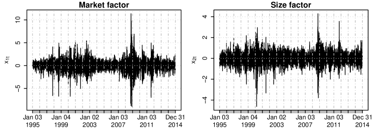
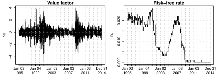
Figure 1: Returns plots of factors and the risk-free rate $R_{f}$

To have a better idea about what the data is like, we plot the observations from 3rd January 1995 to 31st December 2014 of the three factors and the risk-free rate in Figure 1, and the first four components of $Y_{t}$ in Figure 2 corresponding to the industrial sectors Agriculture, Food Products, Candy & Soda, and Beer & Liquor. The plots show clearly that there are periods of large volatility around the 2008-2009 financial crisis. We will see Face performs reasonably well even during that period, whilst the others do not.

We compare the three portfolio allocations, (Face, Sam and Fan), along with the market portfolio, year by year from 1995 to 2014 using a simple trading strategy. For each year we trade on each trading day, which is approximately $T=252$ trading days per year. At the beginning of each year we assume we have an initial balance of $100$ pounds. Although this initial choice is arbitrary, it is a useful way of comparing the performance during the course of a year. We assume no transaction costs, allow for short selling, and assume that all possible portfolio allocations are attainable. Our trading strategy consists of forming a portfolio allocation $\hat{\mbox{\bf w}}$ the end of each trading day and holding it until the end of the next trading day. Between day $t-1$ and day $t$, we obtain the portfolio return

$$R_{t}(\hat{\mbox{\bf w}})=\hat{\mbox{\bf w}}^{\!\mbox{\scriptsize T}}Y_{t}$$

where $\hat{\mbox{\bf w}}$ is formed based on $(X_{t-j}^{\!\mbox{\scriptsize T}},\ Y_{t-j}^{\!\mbox{\scriptsize T}})$, $j=1,\ \cdots,\ n$, for some look-back integer $n$. With the realised returns $R_{t}(\hat{\mbox{\bf w}})$, $t=1,\ \cdots,\ T$, we can calculate the annualized Sharpe ratio

$$\mbox{SR}(\hat{\mbox{\bf w}})=\frac{\bar{R}(\hat{\mbox{\bf w}})}{SD(R)}\sqrt{T},$$

where

$$\bar{R}(\hat{\mbox{\bf w}})=\frac{1}{T}\sum\limits_{t=1}^{T}\left\{R_{t}(\hat{\mbox{\bf w}})-R_{f,t}\right\},\quad SD(R)=\left[\frac{1}{T}\sum\limits_{t=1}^{T}\left\{R_{t}(\hat{\mbox{\bf w}})-R_{f,t}-\bar{R}(\hat{\mbox{\bf w}})\right\}^{2}\right]^{1/2}$$

and $R_{f,t}$ is the risk-free rate on day $t$. Hence, for each year, and for each of the four trading strategies, we compute an annualized Sharpe ratio and the balance at the end of the final trading day of the year. We repeat this using $n=100$, $300$, and $500$. From the the annualized Sharpe ratios presented in Figure 4 and the balances in Table 6, it is clear that Face performs significantly better than the other three.

We remark that although Face, Sam and Fan are all constructed based on Markowitz’s formula, the difference between them lies in the way to estimate the covariance matrix of returns, which appears in Markowitz’s formula. Both Sam and Fan do not take into account the dynamic feature of the covariance matrix in their estimation, but Face does. This is the fundamental reason why Face performs significantly better than Sam and Fan. One may argue that if Sam and Fan used fewer observations in their moving window to estimate the covariance matrix they would start to take the dynamic feature into account, potentially improving their performance. However when constructing Face, Sam and Fan, we tried a variety of $n$, ranging from $100$ to $500$, and found Face always performs better. This suggests that even if Sam and Fan only use the observations in a carefully chosen moving window, Face still outperforms them.

To have a tangible idea about whether the covariance matrix is dynamic or not, we plot the estimated intercept and coefficients of $x_{1,t}$, $x_{2,t}$ and $x_{3,t}$, interpreted as the impact of the factors, for each of the first four components of $Y_{t}$ in Figure 3. One can see that these coefficients are dynamic rather than constant, which implies the covariance matrix is also dynamic.

It is interesting to have a closer look at the performances of the four strategies in the volatile time period 2007-2009 during which the financial crisis took place. Still assuming an initial balance of 100 pounds at the start of each year, and using $n=500$, we plot the balances at the end of each trading day in Figure 5. During 2007, Face, Sam and Fan all perform reasonably well, with Face slightly better. The market does not make much profit, and is beaten by the other three. In 2008, Face continuously does well whilst the other three do not make profit at all. In 2009, although Face does not do very well during some time periods, it adapts to the market change quickly and almost breaks even. The reason that Face can adapt to market change quickly is because it takes into account the dynamic feature of the covariance matrix of returns. On the other hand, both Sam and Fan do very poorly, and in fact they almost lose all their money at the end of the year. In 2009, the market performs best, but still with very little profit.

Table 4: Description of the 49 industry portfolios

$k$	$y_{k,t}$	Industry name		$k$	$y_{k,t}$	Industry name
1	Agric	Agriculture		26	Guns	Defense
2	Food	Food Products		27	Gold	Precious Metals
3	Soda	Candy & Soda		28	Mines	Industrial Metal Mining
4	Beer	Beer & Liquor		29	Coal	Coal
5	Smoke	Tobacco Products		30	Oil	Petroleum and Natural Gas
6	Toys	Recreation		31	Util	Utilities
7	Fun	Entertainment		32	Telcm	Communication
8	Books	Printing and Publishing		33	PerSv	Personal Services
9	Hshld	Consumer Goods		34	BusSv	Business Services
10	Clths	Apparel		35	Hardw	Computers
11	Hlth	Healthcare		36	Softw	Computer Software
12	MedEq	Medical Equipment		37	Chips	Electronic Equipment
13	Drugs	Pharmaceutical Products		38	LabEq	Measuring and Control Equipment
14	Chems	Chemicals		39	Paper	Business Supplies
15	Rubbr	Rubber and Plastic Products		40	Boxes	Shipping Containers
16	Txtls	Textiles		41	Trans	Transportation
17	BldMt	Construction Materials		42	Whlsl	Wholesale
18	Cnstr	Construction		43	Rtail	Retail
19	Steel	Steel Works Etc		44	Meals	Restaurants, Hotels, Motels
20	FabPr	Fabricated Products		45	Banks	Banking
21	Mach	Machinery		46	Insur	Insurance
22	ElcEq	Electrical Equipment		47	RlEst	Real Estate
23	Autos	Automobiles and Trucks		48	Fin	Trading
24	Aero	Aircraft		49	Other	Almost Nothing
25	Ships	Shipbuilding, Railroad Equipment

This table gives the labelling and a brief description of industrial sectors which form the 49 Industry Portfolios data set. Precise details of their construction are given on Kenneth French’s website.

Table 5: Description of the Fama and French factors

$j$	Name of $x_{j,t}$	Description
1	Market factor	Return on the market minus the risk-free rate
2	Size factor	Excess returns of small caps over big caps
3	Value factor	Excess returns of value stocks over growth stocks

This table gives the labelling and a brief description of market, size and value factors from the Fama-French factors data set. Precise details of their construction are given on Kenneth French’s website.

Figure 2: Returns plots of $y_{1,t}$, $y_{2,t}$, $y_{3,t}$, and $y_{4,t}$.

Figure 3: Estimated coefficient functions for industry portfolios 1-4

This figure shows the estimated intercept and coefficient functions for the market, size and value factors, for the first four industry portfolios (Agriculture, Food Products, Candy & Soda, and Beer & Liquor) on the first day of trading.

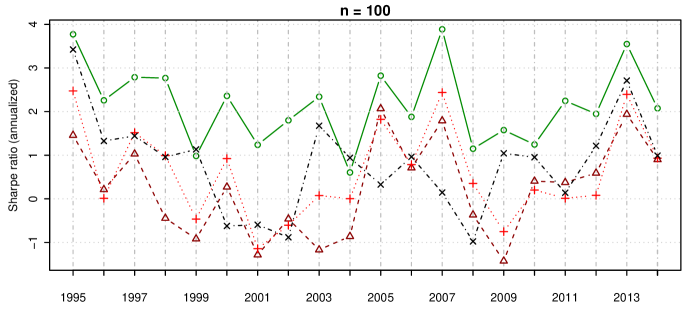
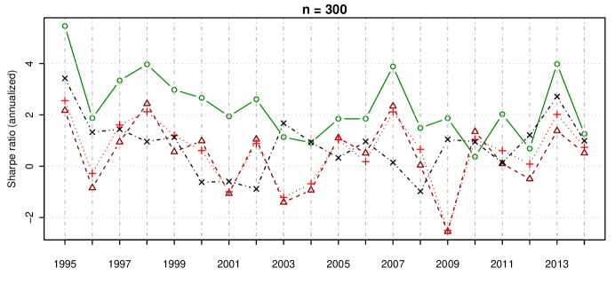
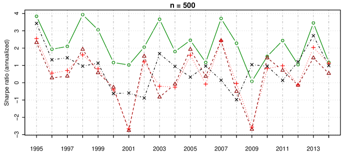
Figure 4: Annualized Sharpe Ratios

This figure shows the performance of the four trading strategies (Face, Sam, Fan and Market) in terms of the annualized Sharpe ratio, using different sample sizes $n=100$, $n=300$ and $n=500$.

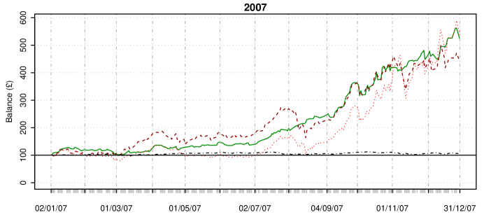
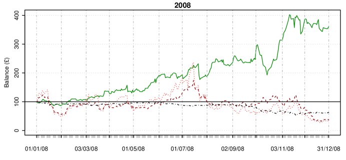
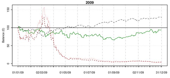
Figure 5: Trading strategies during the financial crisis

This figure shows the performance of the four trading strategies (Face, Sam, Fan and Market) using $n=500$ during 2007, 2008 and 2009 in terms of the end of day balances, assuming an initial balance of 100 pounds at the start of each year.

Table 6: Comparison of Balances of Trading Strategies

Year	Market	$n=100$			$n=300$			$n=500$
		Face	Sam	Fan	Face	Sam	Fan	Face	Sam	Fan
1995	137	224	164	216	541	277	347	423	380	466
1996	121	159	101	96	184	56	72	212	95	115
1997	131	179	138	155	303	146	207	230	98	127
1998	124	178	79	134	317	330	299	442	340	273
1999	126	121	61	78	260	117	175	329	116	135
2000	88	176	102	133	253	155	120	160	54	42
2001	89	129	53	60	167	49	49	140	10	6
2002	79	164	73	69	222	150	142	196	212	176
2003	132	161	57	97	134	40	45	271	53	75
2004	112	112	67	95	132	55	56	180	75	63
2005	106	179	194	166	184	157	151	265	295	239
2006	115	149	119	121	184	114	95	150	103	76
2007	106	233	185	231	376	305	321	521	440	537
2008	63	143	73	104	203	79	114	361	37	32
2009	128	147	48	66	188	9	5	93	4	3
2010	117	129	109	100	107	169	148	152	220	140
2011	100	177	107	93	192	88	120	283	127	154
2012	116	158	117	96	122	60	83	144	71	68
2013	135	232	200	226	412	180	275	389	225	363
2014	112	158	133	134	152	114	131	162	114	178

In this table, the first two columns show the year and the balance on the final trading day when investing in the market portfolio. The balances on the final trading day for Face, Sam and Fan are grouped according to $n=100$ (columns 3-5), $n=300$ (columns 6-8) and $n=500$ (columns 9-11).

APPENDIX

Appendix A: Regularity conditions

We state the following assumptions.

Assumption A1. (i) $\{X_{t}\}_{t\geq 1}$ is stationary and ergodic; (ii) $\{\mbox{\boldmath{$\epsilon$}}_{t}\}_{t\geq 1}$ and $\{X_{t}\}_{t\geq 1}$ are independent; (iii) $X_{t}^{\prime}$s are bounded with support $\mathcal{X}$, that is, $\sup_{t\geq 1}\|X_{t}\|_{\infty}\leq L,a.s$.

Let $P(A)$ be the probability of a measurable set $A$ and $E(X)$ be the expectation of a random variable $X$. The following strong mixing condition (A2) aims at conducting asymptotic properties of the index estimator and local linear estimators of nonparametric functions. Let $\mathcal{F}_{-\infty}^{0}$ and $\mathcal{F}_{k}^{\infty}$ be the $\sigma-$algebras generated by $\{X_{t},t\leq 0\}$ and $\{X_{t},t\geq T\}$, respectively and define the $\alpha-$mixing coefficient

$$\alpha(k)=\sup_{A\in\mathcal{F}_{-\infty}^{0},B\in\mathcal{F}_{k}^{\infty}}\left|P(A)P(B)-P(AB)\right|.$$

Assumption A2. There exist positive constants $c$ and $0<\rho<1$ such that for all $k=1,2,\cdots,$

$$\alpha(k)\leq c\rho^{-k}.$$

Assumption A3. (i) The kernel function $K(z)$ is a symmetric density function which is bounded with a bounded support and satisfies the Lipschitz condition; (ii) The density function $f_{\mbox{\bf b}}(z)$ of $X^{\!\mbox{\scriptsize T}}\mbox{\bf b}$ is twice differentiable and bounded away from zero on $\{z=\mbox{\bf x}^{\!\mbox{\scriptsize T}}\mbox{\bf b};\mbox{\bf x}\in\mathcal{X},\|\mbox{\bf b}-\mbox{\boldmath{$\beta$}}\|_{2}\leq c_{0}\}$ with $0<c_{0}<1$; (iii) The density function $f(\mbox{\bf x})$ of $X_{t}$ is bounded away from zero and twice differentiable in $\mathcal{X}$ and the joint densities of $X_{1}$ and $X_{k}$ for all $k\geq 2$ are bounded.

Assumption A4. $\mbox{\bf g}(z)$ and $\mbox{\boldmath{$\Phi$}}(z)$ have continuous third derivatives in $\mathcal{Z}=\{z:z=\mbox{\bf x}^{\!\mbox{\scriptsize T}}\mbox{\boldmath{$\beta$}},\mbox{\bf x}\in\mathcal{X}\}.$

Assumption A5. $\|\mbox{\bf V}_{p}-\mbox{\bf V}\|=o(1)$, as $p_{n}\to\infty$, for some $q\times q$ symmetric positive definite V such that $\lambda_{\min}(\mbox{\bf V})$ is bounded away from zero.

For the error process $\{\mbox{\boldmath{$\epsilon$}}_{t},t\geq 1\}$, the following assumptions are stated. Denote the true value $\mbox{\boldmath{$\theta$}}_{\ell}=(\alpha_{\ell,0},\cdots,\alpha_{\ell,m},\gamma_{\ell,1},\cdots,\gamma_{\ell,s})^{\!\mbox{\scriptsize T}}$ for $\ell=1,\cdots,p_{n}$.

Assumption B1. For each $\ell=1\cdots,p_{n}$, $\{(\epsilon_{\ell,t},\sigma_{\ell,t}^{2}),t=0,\pm 1,\pm 2,\cdots\}$ is a strictly stationary GARCH$(m,s)$ process with $\sup_{1\leq\ell\leq p_{n}}E\sigma_{\ell,1}^{2d}<\infty$ with $d>4$.

Assumption B2. Let $\eta_{\ell,t}=\sigma_{\ell,t}^{-1}\epsilon_{\ell,t}$ for each $t$ and $\ell$. Then, for each $\ell=1,\cdots,p_{n},$ the innovations $\eta_{\ell,t}$’s are $i.i.d.$ and absolutely continuous with Lebesgue density being strictly positive in a neighbourhood of zero. Furthermore, $E\eta_{\ell,1}=0$, $E\eta_{\ell,1}^{2}=1$ and $\sup_{\ell\leq p_{n}}E(\eta_{\ell,1}^{2d})<\infty$ with $d$ defined in Assumption (B1).

Assumption B3. For each $\ell=1,\cdots,p_{n}$, the true value $\mbox{\boldmath{$\theta$}}_{\ell,0}$ is an interior point of the compact set $\Lambda$ and $\mbox{\boldmath{$\Lambda$}}\subset(c,+\infty)\times(c,+\infty)^{m+s}$ for a constant $c>0$.

Assumption B4. Let $\mathcal{A}_{\ell,\theta}(z)=\sum_{i=1}^{m}\alpha_{\ell,i}z^{i}$ and $\mathcal{B}_{\ell,\theta}(z)=1-\sum_{i=1}^{s}\gamma_{\ell,i}z^{i}$ for $\ell=1,\cdots,p_{n}$. If $s>0$, $\mathcal{A}_{\ell,\theta_{\ell,0}}(z)$ and $\mathcal{B}_{\ell,\theta_{\ell,0}}(z)$ have no common roots, $\mathcal{A}_{\ell,\theta_{\ell,0}}(1)\neq 0$, and $\alpha_{\ell,0m}+\gamma_{\ell,0s}\neq 0$.

For the bandwidths $h$, $h_{1}$, $h_{2}$ and the dimension $p_{n}$, we require the following assumptions.

Assumption C1. (i) The bandwidth $h$ and $h_{1}$ satisfy $h=O(n^{-\tau})$ and $h_{1}=O(n^{-\tau_{1}})$, respectively, with $1/6<\tau,\tau_{1}<1/4$.

Assumption C2. The bandwidth $h_{2}$ satisfies $h_{2}=O(n^{-\tau_{2}})$ with $1/(2q+4)<\tau_{2}<1/(2q+2)$.

Assumption C3. The dimension $p_{n}$ satisfies $p_{n}\leq Cn^{d/2-2-2\varepsilon}$ for some constants $C>0$ and $0<2\varepsilon<d/2-2$.

Our aim is to estimate $\mbox{cov}(Y_{t}|\mathcal{F}_{t-1})$. Fan, Fan and Lv (2008) and Fan, Liao and Mincheva (2013) showed that by incorporating the factor structure into the covariance matrix, the resulting estimator has a better convergence rate than the usual sample covariance matrix under the norm $\|\cdot\|_{\boldsymbol{\Sigma}}$. To prove the convergence rate of $\widehat{\mbox{cov}}(Y_{t}|\mathcal{F}_{t-1})-\mbox{cov}(Y_{t}|\mathcal{F}_{t-1})$ under the norm $\|\cdot\|_{\boldsymbol{\Sigma}}$, we impose the following assumption:

Assumption C4. For each $\mbox{\bf x}\in\mathcal{X}$, $\|p_{n}^{-1}\{\mbox{\boldmath{$\Phi$}}(\mbox{\bf x}^{\!\mbox{\scriptsize T}}\mbox{\boldmath{$\beta$}})\}^{\!\mbox{\scriptsize T}}\mbox{\boldmath{$\Phi$}}(\mbox{\bf x}^{\!\mbox{\scriptsize T}}\mbox{\boldmath{$\beta$}})-\mbox{\bf V}_{2}\|=o(1)$, as $p_{n}\to\infty$ for some $q\times q$ symmetric positive definite $\mbox{\bf V}_{2}$ such that $\lambda_{\min}(\mbox{\bf V}_{2})$ is bounded away from zero.

The assumptions are regular. The strong mixing condition in the Assumption (A2) can be relaxed as $\alpha(k)\leq ck^{-\beta}$ with a large constant $\beta$. Assumption (B1) and (B2) guarantee the existence of the $2d-$th moment of $\epsilon_{\ell,1}$. For simplicity, we do not impose the conditions that ensure the finiteness of the $d-$th moment of $\sigma_{\ell,1}^{2}$. For more details, see Lindner (2009). Assumption (C4) requires that the factors should be pervasive, that is, impact every individual time series. It was also imposed in Fan, Fan and Lv (2008) and Fan, Liao and Mincheva (2011).

Appendix B: Proof of Theorem 1 (I)-(III)

For ease of presentation, we give some notation. Define

$$\delta_{\textbf{b}}=\|\mbox{\bf b}-\mbox{\boldmath{$\beta$}}\|,\delta_{1n}=\left(\frac{\log(n)}{nh}\right)^{1/2},\delta_{2n}=\left(\frac{\log(n)}{n}\right)^{1/2},\delta_{3n}=\left(\frac{\log(n)}{nh_{1}}\right)^{1/2}$$

and $\tilde{\delta}_{n}=h^{3}+h^{2}\delta_{1n}+\delta_{1n}^{2}.$ Define $\Theta$ to be a compact set $\{\mbox{\bf b}:\|\mbox{\bf b}-\mbox{\boldmath{$\beta$}}\|\leq c_{0},\|\mbox{\bf b}\|=1\}$ with a small $c_{0}>0$. For a random sequence $a_{n}$, $a_{n}=\bar{O}_{a.s.}(b_{n})$ for some sequence $b_{n}$ means that $P\left\{\|a_{n}\|>Cb_{n}\right\}=O({n^{-(1+\varepsilon)}}),$ where $\varepsilon$ is defined in Assumption (C3).

To prove Theorem 1, the following lemma is useful.

Lemma B.1. Assume that Conditions (A1)-(A3) and (C3) in Appendix A hold and for some $d>4$,

$$\sup_{1\leq\ell\leq p_{n}}E|\epsilon_{\ell,t}|^{2d}<\infty,$$

where $d$ is defined in (C3). Then there exists a constant $C>0$ such that

$$P\left\{\sup_{1\leq\ell\leq p_{n}}\sup_{(\mbox{\bf b},\mbox{\bf x})\in(\boldsymbol{\Theta},\mathcal{X})}\left|\frac{1}{n}\sum_{t=1}^{n}K_{h}(X_{i}^{\!\mbox{\scriptsize T}}\mbox{\bf b}-\mbox{\bf x}^{\!\mbox{\scriptsize T}}\mbox{\bf b})\epsilon_{\ell,t}\right|>C\delta_{1n}\right\}\leq O\left(\frac{1}{n^{1+\varepsilon}}\right).$$

The proof of Lemma B.1 can be followed from the proof of Lemma 6.1 in Fan and Yao (2003). Of course, some constants involved in the proof need to be modified. For instance, we instead use $B_{n}=(nh)^{1/2}(\log(n))^{-2}$.

Denote $Y=\left(Y_{2},\ \cdots,\ Y_{n}\right),$ $W_{h}(z;\mbox{\bf b})=\mbox{diag}\left\{K_{h}(X_{1}^{\!\mbox{\scriptsize T}}\mbox{\bf b}-z),\ \cdots,\ K_{h}(X_{n-1}^{\!\mbox{\scriptsize T}}\mbox{\bf b}-z)\right\}$ and

$$\widetilde{X}(z;\mbox{\bf b})=\left(\begin{array}[]{c}\widetilde{X}_{2}^{\!\mbox{\scriptsize T}}(z;\mbox{\bf b})\\ \vdots\\ \widetilde{X}_{n}^{\!\mbox{\scriptsize T}}(z;\mbox{\bf b})\end{array}\right)=\left(\begin{array}[]{cccc}1&X_{2}^{\!\mbox{\scriptsize T}}&X_{1}^{\!\mbox{\scriptsize T}}\mbox{\bf b}-z&(X_{1}^{\!\mbox{\scriptsize T}}\mbox{\bf b}-z)X_{2}^{\!\mbox{\scriptsize T}}\\ \vdots&\vdots&\vdots&\vdots\\ 1&X_{n}^{\!\mbox{\scriptsize T}}&X_{n-1}^{\!\mbox{\scriptsize T}}\mbox{\bf b}-z&(X_{n-1}^{\!\mbox{\scriptsize T}}\mbox{\bf b}-z)X_{n}^{\!\mbox{\scriptsize T}}\end{array}\right),$$

Let $H=\mbox{diag}(\mbox{\bf 1}_{1\times(q+1)},h\mbox{\bf 1}_{1\times(q+1)})$ and denote $\widehat{\Omega}_{h}(z;\mbox{\bf b})=H^{-1}\{\widetilde{X}(z;\mbox{\bf b})\}^{\!\mbox{\scriptsize T}}W_{h}(z;\mbox{\bf b})\widetilde{X}(z;\mbox{\bf b})H^{-1}.$ Denote $\mu_{2}=\int u^{2}K(u)du$, $\mbox{\boldmath{$\mu$}}_{\textbf{b}}(z)=E(X|X^{\!\mbox{\scriptsize T}}\mbox{\bf b}=z)$ and, for $\ell=1,\cdots,p_{n}$, $\tilde{\mbox{\boldmath{$\epsilon$}}}_{\ell}=(\epsilon_{\ell,2},\cdots,\epsilon_{\ell,n})^{\!\mbox{\scriptsize T}}$,

$$\widehat{\mbox{\boldmath{$\Gamma$}}}_{\ell}(z;\mbox{\bf b}) = H^{-1}\left\{\widehat{\Omega}_{h}(z;\mbox{\bf b})\right\}^{-1}H^{-1}\widetilde{X}^{\!\mbox{\scriptsize T}}(z;\mbox{\bf b})W_{h}(z;\mbox{\bf b})\mbox{\bf y}_{\ell},\mbox{\boldmath{$\Gamma$}}_{\ell}(z)=(g_{\ell}(z),(\mbox{\boldmath{$\Phi$}}_{\ell}(z))^{\!\mbox{\scriptsize T}},\dot{g}_{\ell}(z),(\dot{\mbox{\boldmath{$\Phi$}}}_{\ell}(z))^{\!\mbox{\scriptsize T}})^{\!\mbox{\scriptsize T}},$$

$$\mbox{\boldmath{$\Gamma$}}^{\prime}_{\ell}(z) = (\dot{g}_{\ell}(z),(\dot{\mbox{\boldmath{$\Phi$}}}_{\ell}(z))^{\!\mbox{\scriptsize T}},\ddot{g}_{\ell}(z),(\ddot{\mbox{\boldmath{$\Phi$}}}_{\ell}(z))^{\!\mbox{\scriptsize T}})^{\!\mbox{\scriptsize T}},\mbox{\boldmath{$\Gamma$}}^{\prime\prime}_{\ell}(z)=(\ddot{g}_{\ell}(z),(\ddot{\mbox{\boldmath{$\Phi$}}}_{\ell}(z))^{\!\mbox{\scriptsize T}},\mbox{\bf 0}_{1\times(q+1)})^{\!\mbox{\scriptsize T}}.$$

The following lemma gives the asymptotic representation of $\widehat{\mbox{\boldmath{$\Gamma$}}}_{\ell}(z)$.

Lemma B.2. Suppose that Assumption (A1)-(A4) in Appendix A hold. Then we have that

$$H\widehat{\mbox{\boldmath{$\Gamma$}}}_{\ell}(z;\mbox{\bf b}) = H\mbox{\boldmath{$\Gamma$}}_{\ell}(z)+\big{\{}\widehat{\Omega}_{h}(z;\mbox{\bf b})\big{\}}^{-1}H^{-1}\widetilde{X}^{\!\mbox{\scriptsize T}}(z;\mbox{\bf b})W_{h}(z;\mbox{\bf b})\tilde{\mbox{\boldmath{$\epsilon$}}}_{\ell}+H\mbox{\boldmath{$\Gamma$}}^{\prime}_{\ell}(z)\big{(}\mbox{\boldmath{$\mu$}}_{\textbf{b}}(z)\big{)}^{\!\mbox{\scriptsize T}}(\mbox{\boldmath{$\beta$}}-\mbox{\bf b})$$

$$+\frac{1}{2}\mu_{2}h^{2}H\mbox{\boldmath{$\Gamma$}}^{\prime\prime}_{\ell}(z)+\bar{O}_{a.s.}\big{(}h\delta_{\textbf{b}}+\delta_{1n}\delta_{\textbf{b}}+\delta_{\textbf{b}}^{2}+\tilde{\delta}_{n}\big{)}.$$

Proof of Lemma B.2. For $i=2,\cdots,n$, denote $z_{i}=X_{i-1}^{\!\mbox{\scriptsize T}}\mbox{\boldmath{$\beta$}}$ and $z_{\textbf{b},i}=X_{i-1}^{\!\mbox{\scriptsize T}}\mbox{\bf b}$. Using a Taylor’s expansion, we obtain that

$$y_{\ell,i}=g_{\ell}(z_{i})+\mbox{\boldmath{$\Phi$}}_{\ell}(z_{i})X_{i}+\epsilon_{\ell,i}=\widetilde{X}_{i}^{\!\mbox{\scriptsize T}}(z;\mbox{\bf b})\mbox{\boldmath{$\Gamma$}}_{\ell}(z)+\epsilon_{\ell,i}+r_{\ell,\textbf{b},i}^{(1)}+r_{\ell,\textbf{b},i}^{(2)}+r_{\ell,\textbf{b},i}^{(3)}+r_{\ell,\textbf{b},i}^{(4)},$$

where $r_{\ell,\textbf{b},i}^{(1)}=\widetilde{X}_{\textbf{b},i}^{\!\mbox{\scriptsize T}}(z)\mbox{\boldmath{$\Gamma$}}^{\prime}_{\ell}(z)(z_{i}-z_{\textbf{b},i}),r_{\ell,\textbf{b},i}^{(2)}=2^{-1}\widetilde{X}_{\textbf{b},i}^{\!\mbox{\scriptsize T}}(z)\mbox{\boldmath{$\Gamma$}}^{\prime\prime}_{\ell}(z)(z_{\textbf{b},i}-z)^{2},$
$r_{\ell,\textbf{b},i}^{(3)}=2^{-1}\widetilde{X}_{\textbf{b},i}^{\!\mbox{\scriptsize T}}(z)\mbox{\boldmath{$\Gamma$}}^{\prime\prime}_{\ell}(z)(z_{i}-z_{\textbf{b},i})^{2},r_{\ell,\textbf{b},i}^{(4)}=O(|z_{i}-z|^{3}).$

For $k=1,\cdots,4$, denote $\mbox{\bf r}_{\ell,\textbf{b}}^{(k)}=(\mbox{\bf r}_{\ell,\textbf{b},2}^{(k)},\cdots,\mbox{\bf r}_{\ell,\textbf{b},n}^{(k)})^{\!\mbox{\scriptsize T}}$. Then

$$H\widehat{\mbox{\boldmath{$\Gamma$}}}_{\ell}(z;\mbox{\bf b})-H\mbox{\boldmath{$\Gamma$}}_{\ell}(z)=\left\{\widehat{\Omega}_{h}(z;\mbox{\bf b})\right\}^{-1}H^{-1}\widetilde{X}^{\!\mbox{\scriptsize T}}(z;\mbox{\bf b})W_{h}(z;\mbox{\bf b})\left(\tilde{\mbox{\boldmath{$\epsilon$}}}_{\ell}+\mbox{\bf r}_{\ell,\textbf{b}}^{(1)}+\mbox{\bf r}_{\ell,\textbf{b}}^{(2)}+\mbox{\bf r}_{\ell,\textbf{b}}^{(3)}+\mbox{\bf r}_{\ell,\textbf{b}}^{(4)}\right).$$

(I). Consider the term $\widehat{\Omega}_{h}(z;\mbox{\bf b})$. Following the proof of Theorem 5.3 in Fan and Yao (2003), we have that there exists a large $C>0$ such that

$$P\left\{\sup_{(\textbf{b},z)\in\boldsymbol{\Theta}\times\mathcal{Z}}\left\|{1\over n}\left(\widehat{\Omega}_{h}(z;\mbox{\bf b})-E\left\{\widehat{\Omega}_{h}(z;\mbox{\bf b})\right\}\right)\right\|_{F}>C\delta_{1n}\right\}\leq O\left({1\over n^{2}}\right).$$

Let $\Omega(z;\mbox{\bf b})=\lim_{n\to\infty}n^{-1}E\left\{\widehat{\Omega}_{h}(z;\mbox{\bf b})\right\}$. Note that $n^{-1}E\widehat{\Omega}_{h}(z;\mbox{\bf b})=\Omega(z;\mbox{\bf b})+O(h)$ and $\Omega(z;\mbox{\bf b})$ is positive definite. Therefore, $\widehat{\Omega}_{h}(z;\mbox{\bf b})$ is positive definite almost surely and

$$n^{-1}\widehat{\Omega}_{h}(z;\mbox{\bf b})=\Omega(z;\mbox{\bf b})+\bar{O}_{a.s.}(h+\delta_{1n}).$$

(II). Consider the term $H^{-1}\widetilde{X}^{\!\mbox{\scriptsize T}}(z;\mbox{\bf b})W_{h}(z;\mbox{\bf b})\mbox{\bf r}_{\textbf{b},\ell}^{(k)}$ $(k=1,\cdots,4)$. By specific matrix calculations, we can show that

$$H^{-1}\widetilde{X}^{\!\mbox{\scriptsize T}}(z;\mbox{\bf b})W_{h}(z;\mbox{\bf b})\mbox{\bf r}_{\textbf{b},\ell}^{(1)} = \Omega(z;\mbox{\bf b})H\mbox{\boldmath{$\Gamma$}}^{\prime}_{\ell}(z)\big{(}\mbox{\boldmath{$\mu$}}_{\textbf{b}}(z)\big{)}^{\!\mbox{\scriptsize T}}(\mbox{\boldmath{$\beta$}}-\mbox{\bf b})+\bar{O}_{a.s.}\Big{(}h\delta_{\textbf{b}}+\delta_{1n}\delta_{\textbf{b}}\Big{)},$$

$$H^{-1}\widetilde{X}^{\!\mbox{\scriptsize T}}(z;\mbox{\bf b})W_{h}(z;\mbox{\bf b})\mbox{\bf r}_{\textbf{b},\ell}^{(2)} = \frac{1}{2}\mu^{2}h^{2}\Omega_{(}z;\mbox{\bf b})H\mbox{\boldmath{$\Gamma$}}^{\prime\prime}_{\ell}(z)+\bar{O}_{a.s.}\Big{(}h^{3}+h^{2}\delta_{1n}\Big{)},$$

$$H^{-1}\widetilde{X}^{\!\mbox{\scriptsize T}}(z;\mbox{\bf b})W_{h}(z;\mbox{\bf b})\mbox{\bf r}_{\textbf{b},\ell}^{(3)} = \bar{O}_{a.s.}\big{(}\delta_{\textbf{b}}^{2}\big{)},\ \ H^{-1}\widetilde{X}^{\!\mbox{\scriptsize T}}(z;\mbox{\bf b})W_{h}(z;\mbox{\bf b})\mbox{\bf r}_{\textbf{b},\ell}^{(4)}=\bar{O}_{a.s.}\big{(}\delta_{\textbf{b}}^{3}+h^{3}+h^{2}\delta_{\textbf{b}}+h\delta_{\textbf{b}}^{2}\big{)}.$$

Combining (I) and (II), we obtain that

$$H\widehat{\mbox{\boldmath{$\Gamma$}}}_{\ell}(z;\mbox{\bf b}) = H\mbox{\boldmath{$\Gamma$}}_{\ell}(z)+\big{\{}\widehat{\Omega}_{h}(z;\mbox{\bf b})\big{\}}^{-1}H^{-1}\widetilde{X}^{\!\mbox{\scriptsize T}}(z;\mbox{\bf b})W_{h}(z;\mbox{\bf b})\tilde{\mbox{\boldmath{$\epsilon$}}}_{\ell}+H\mbox{\boldmath{$\Gamma$}}^{\prime}_{\ell}(z)\big{(}\mbox{\boldmath{$\mu$}}_{\textbf{b}}(z)\big{)}^{\!\mbox{\scriptsize T}}(\mbox{\boldmath{$\beta$}}-\mbox{\bf b})$$

$$+\frac{1}{2}\mu^{2}h^{2}H\mbox{\boldmath{$\Gamma$}}^{\prime\prime}_{\ell}(z)+\bar{O}_{a.s.}\big{(}h\delta_{\textbf{b}}+\delta_{1n}\delta_{\textbf{b}}+\delta_{\textbf{b}}^{2}+\tilde{\delta}_{n}\big{)}.$$

This completes the proof.

The following lemma, Lemma B.3, gives the asymptotic relationship between $\widehat{\mbox{\boldmath{$\beta$}}}_{m+1}$ and $\widehat{\mbox{\boldmath{$\beta$}}}_{m}$, where $\widehat{\mbox{\boldmath{$\beta$}}}_{m}$ is the $m$th step estimator based on our procedure in Section 2.

Without loss of generality, we consider $m=1$. For each $i,j=1,\cdots,n-1$, define

$$X_{ij}=X_{i}-X_{j},w_{ij}(\mbox{\bf b})=h^{-1}K\left\{X_{ij}^{\!\mbox{\scriptsize T}}\mbox{\bf b}/{h}\right\}.$$

Given $\widehat{\boldsymbol{\beta}}_{1}$, for $j=1,\cdots,n-1$, denote $\hat{z}_{j}=X_{j}^{\!\mbox{\scriptsize T}}\widehat{\boldsymbol{\beta}}_{1}$ and

$$\widehat{\mbox{\boldmath{$\Gamma$}}}_{j}=(\widehat{\mbox{\bf g}}_{j},\widehat{\mbox{\boldmath{$\xi$}}}_{j},\widehat{A}_{j},\widehat{B}_{j})=YW_{h}(\hat{z}_{j};\widehat{\boldsymbol{\beta}}_{1})\widetilde{X}(\hat{z}_{j};\widehat{\boldsymbol{\beta}}_{1})\left\{\widetilde{X}^{\!\mbox{\scriptsize T}}(\hat{z}_{j};{\widehat{\boldsymbol{\beta}}_{1}})W_{h}(\hat{z}_{j};\widehat{\boldsymbol{\beta}}_{1})\widetilde{X}(\hat{z}_{j};{\widehat{\boldsymbol{\beta}}_{1}})\right\}^{-1}.$$

and

$$\widehat{\mbox{\bf V}}_{n} = \frac{1}{n^{2}p_{n}}\sum_{i,j=1}^{n-1}X_{ij}X_{ij}^{\!\mbox{\scriptsize T}}\|\widehat{\mbox{\boldmath{$\xi$}}}_{j}+\widehat{B}_{j}X_{i+1}\|^{2}w_{ij}(\widehat{\mbox{\boldmath{$\beta$}}}_{1}),$$

$$\widehat{\mbox{\bf U}}_{n} = \frac{1}{n^{2}p_{n}}\sum_{i,j=1}^{n-1}X_{ij}\Big{(}\widehat{\mbox{\boldmath{$\xi$}}}_{j}+\widehat{B}_{j}X_{i+1}\Big{)}^{\!\mbox{\scriptsize T}}\Big{\{}Y_{i+1}-\widehat{\mbox{\boldmath{$\Gamma$}}}_{j}\widetilde{X}(\hat{z}_{j};\widehat{\mbox{\boldmath{$\beta$}}}_{1})\Big{\}}w_{ij}(\widehat{\mbox{\boldmath{$\beta$}}}_{1}),$$

$$\widehat{\mbox{\boldmath{$\beta$}}}_{2} = \widehat{\mbox{\boldmath{$\beta$}}}_{1}+\widehat{\mbox{\bf V}}^{-1}_{n}\widehat{\mbox{\bf U}}_{n}.$$

Lemma B.3. Suppose that Conditions (A1)-(A4), (B1)-(B4), (C1) and (C3) in Appendix A hold. Then, we have

$$\widehat{\mbox{\boldmath{$\beta$}}}_{2}-\mbox{\boldmath{$\beta$}}=\frac{1}{2}\left(\widehat{\mbox{\boldmath{$\beta$}}}_{1}-\mbox{\boldmath{$\beta$}}\right)+\frac{1}{2}\mbox{\bf V}_{p}^{-1}\mbox{\bf U}_{n}+\mbox{\bf R}_{n},$$ (A.1)

where $\mbox{\bf R}_{n}=\bar{O}_{a.s.}\left(h\delta_{2n}+h^{-1}\delta_{2n}^{2}+\tilde{\delta}_{n}+h^{-1}\delta_{2n}\delta_{\widehat{\boldsymbol{\beta}}_{1}}+h\delta_{\widehat{\boldsymbol{\beta}}_{1}}+h^{-1}\delta^{2}_{\widehat{\boldsymbol{\beta}}_{1}}\right).$

Proof of Lemma B.3. First, consider the term $\mbox{\bf U}_{n}$. For $i,j=1,\cdots,n-1,$ denote

$$\mbox{\bf e}_{ij,1} = \mbox{\bf g}^{\prime}(X_{j}^{\!\mbox{\scriptsize T}}\mbox{\boldmath{$\beta$}})+\mbox{\boldmath{$\Phi$}}^{\prime}(X_{j}^{\!\mbox{\scriptsize T}}\mbox{\boldmath{$\beta$}})X_{i+1},\mbox{\bf e}_{ij,2}=\widehat{\mbox{\boldmath{$\xi$}}}_{j}+\widehat{\mbox{\bf B}}_{j}X_{i+1}-\mbox{\bf e}_{ij,1},$$

$$\mbox{\bf e}_{i,3} = \mbox{\bf g}(\hat{z}_{i})+\mbox{\boldmath{$\Phi$}}(\hat{z}_{i})X_{i+1}+(\mbox{\bf g}^{\prime}(\hat{z}_{i})+\mbox{\boldmath{$\Phi$}}^{\prime}(\hat{z}_{i})X_{i+1})(\mbox{\boldmath{$\mu$}}_{\boldsymbol{\beta}}(X_{i}^{\!\mbox{\scriptsize T}}\mbox{\boldmath{$\beta$}}))^{\!\mbox{\scriptsize T}}(\mbox{\boldmath{$\beta$}}-\widehat{\mbox{\boldmath{$\beta$}}}_{1}),$$

$$\mbox{\bf e}_{ij,4} = \widehat{\mbox{\boldmath{$\Gamma$}}}_{j}\widetilde{X}_{i+1}(\hat{z}_{j};\widehat{\mbox{\boldmath{$\beta$}}}_{1})-\mbox{\bf e}_{i,3}.$$

We decompose $\widehat{\mbox{\bf U}}_{n}$ as

$$\widehat{\mbox{\bf U}}_{n} = \frac{1}{n^{2}p_{n}}\sum_{i,j=1}^{n-1}X_{ij}\mbox{\bf e}_{ij,1}^{\!\mbox{\scriptsize T}}\big{(}Y_{i+1}-\mbox{\bf e}_{i,3}\big{)}w_{ij}(\widehat{\mbox{\boldmath{$\beta$}}}_{1})-\frac{1}{n^{2}p_{n}}\sum_{i,j=1}^{n-1}X_{ij}\mbox{\bf e}_{ij,1}^{\!\mbox{\scriptsize T}}\mbox{\bf e}_{j,4}w_{ij}(\widehat{\mbox{\boldmath{$\beta$}}}_{1})$$

$$+\frac{1}{n^{2}p_{n}}\sum_{i,j=1}^{n-1}X_{ij}\mbox{\bf e}_{ij,2}^{\!\mbox{\scriptsize T}}\big{(}Y_{i+1}-\mbox{\bf e}_{i,3}\big{)}w_{ij}(\widehat{\mbox{\boldmath{$\beta$}}}_{1})-\frac{1}{n^{2}p_{n}}\sum_{i,j=1}^{n-1}X_{ij}\mbox{\bf e}_{ij,2}^{\!\mbox{\scriptsize T}}\mbox{\bf e}_{ij,4}w_{ij}(\widehat{\mbox{\boldmath{$\beta$}}}_{1})=\sum_{k=1}^{4}\mbox{\bf U}_{nk}.$$

(a). Consider the main term $\mbox{\bf U}_{n1}$. Note that

$$Y_{i+1}-\mbox{\bf e}_{i,3}=\mbox{\boldmath{$\epsilon$}}_{i+1}+\left(\mbox{\bf g}^{\prime}(X_{i}^{\!\mbox{\scriptsize T}}\mbox{\boldmath{$\beta$}})+\mbox{\boldmath{$\Phi$}}^{\prime}(X_{i}^{\!\mbox{\scriptsize T}}\mbox{\boldmath{$\beta$}})X_{i+1}\right)\big{(}X_{i}-\mbox{\boldmath{$\mu$}}_{\boldsymbol{\beta}}(X_{i}^{\!\mbox{\scriptsize T}}\mbox{\boldmath{$\beta$}})\big{)}^{\!\mbox{\scriptsize T}}(\mbox{\boldmath{$\beta$}}-\widehat{\mbox{\boldmath{$\beta$}}}_{1})+O(\delta_{\widehat{\boldsymbol{\beta}}_{1}}^{2}).$$

Analogous to Lemma A.2 of Xia, Tong and Li (2002), it follows that

$$\frac{1}{n^{2}p_{n}}\sum_{i,j=1}^{n-1}X_{ij}\mbox{\bf e}_{ij,1}^{\!\mbox{\scriptsize T}}\mbox{\boldmath{$\epsilon$}}_{i+1}w_{ij}(\widehat{\mbox{\boldmath{$\beta$}}}_{1})=\mbox{\bf U}_{n}+\bar{O}_{a.s.}(\delta_{1n}\delta_{\widehat{\boldsymbol{\beta}}_{1}}).$$

Similarly, we obtain that

$$\frac{1}{n^{2}p_{n}}\sum_{i,j=1}^{n-1}X_{ij}\mbox{\bf e}_{ij,1}^{\!\mbox{\scriptsize T}}\left(\mbox{\bf g}^{\prime}(X_{i}^{\!\mbox{\scriptsize T}}\mbox{\boldmath{$\beta$}})+\mbox{\boldmath{$\Phi$}}^{\prime}(X_{i}^{\!\mbox{\scriptsize T}}\mbox{\boldmath{$\beta$}})X_{i+1}\right)\big{(}X_{i}-\mbox{\boldmath{$\mu$}}_{\boldsymbol{\beta}}(X_{i}^{\!\mbox{\scriptsize T}}\mbox{\boldmath{$\beta$}})\big{)}^{\!\mbox{\scriptsize T}}w_{ij}(\widehat{\mbox{\boldmath{$\beta$}}}_{1})=\mbox{\bf V}_{p}+\bar{O}_{a.s.}(\delta_{1n}+\delta_{\widehat{\boldsymbol{\beta}}_{1}}).$$

Hence, we approximate the term $\mbox{\bf U}_{n1}$ as

$$\mbox{\bf U}_{n1}=\mbox{\bf U}_{n}+{\mbox{\bf V}}_{p}(\mbox{\boldmath{$\beta$}}-\widehat{\mbox{\boldmath{$\beta$}}}_{1})+\bar{O}_{a.s.}\big{(}\delta_{1n}\delta_{\widehat{\boldsymbol{\beta}}_{1}}+\delta_{\widehat{\boldsymbol{\beta}}_{1}}^{2}\big{)}.$$

(b). With the help of asymptotic representation of $\widehat{\mbox{\boldmath{$\Gamma$}}}_{j}(z)$ and empirical approximation theories, we can show that

$$\mbox{\bf U}_{nk}=\bar{O}_{a.s.}\big{(}h\delta_{\widehat{\boldsymbol{\beta}}_{1}}+h^{-1}\delta_{2n}\delta_{\widehat{\boldsymbol{\beta}}_{1}}+h^{-1}\delta_{\widehat{\boldsymbol{\beta}}_{1}}^{2}+\tilde{\delta}_{n}\big{)},k=2,3,4.$$

(c). In the similar fashion, we can also show that

$$\widehat{\mbox{\bf V}}_{n}=2\mbox{\bf V}_{p}+\bar{O}_{a.s.}\left(\delta_{\widehat{\boldsymbol{\beta}}_{1}}+h+h^{-1}\delta_{2n}\right).$$

Therefore, $\widehat{\mbox{\boldmath{$\beta$}}}_{2}-\widehat{\mbox{\boldmath{$\beta$}}}_{1}=2^{-1}(\mbox{\boldmath{$\beta$}}-\widehat{\mbox{\boldmath{$\beta$}}}_{1})+2^{-1}{\mbox{\bf V}}_{p}^{-1}{\mbox{\bf U}}_{n}+\mbox{\bf R}_{n},$ which means that

$$\widehat{\mbox{\boldmath{$\beta$}}}_{2}-\mbox{\boldmath{$\beta$}}=\frac{1}{2}(\widehat{\mbox{\boldmath{$\beta$}}}_{1}-\mbox{\boldmath{$\beta$}})+\frac{1}{2}{\mbox{\bf V}}_{p}^{-1}{\mbox{\bf U}}_{n}+\mbox{\bf R}_{n}.$$ (A.2)

This completes the proof.

Proof of Theorem 1 (I). First, by Lemma B.3, for the $m-$th step ($m>1$), we have

$$\widehat{\mbox{\boldmath{$\beta$}}}_{m+1}-\mbox{\boldmath{$\beta$}}=\frac{1}{2}(\widehat{\mbox{\boldmath{$\beta$}}}_{m}-\mbox{\boldmath{$\beta$}})+\frac{1}{2}\mbox{\bf V}_{p}^{-1}{\mbox{\bf U}}_{n}+\mbox{\bf R}_{n,m},$$ (A.3)

where $\|\mbox{\bf R}_{n,m}\|\leq M\left(\delta_{\widehat{\boldsymbol{\beta}}_{m}}(h+h^{-1}\delta_{2n}+h^{-1}\delta_{\widehat{\boldsymbol{\beta}}_{m}})+\tilde{\delta}_{n}+h\delta_{2n}+h^{-1}\delta_{2n}^{2}\right)$ a.s. and
$\|{\mbox{\bf V}}_{p}^{-1}{\mbox{\bf U}}_{n}\|\leq M\delta_{2n}$ a.s., with some large positive constant $M$. Here we take $M>1$ and $h<1$ for sufficiently large $n$. Note that as $n\to\infty$, the bandwidth $h$ satisfies $h\to 0$, $h^{-1}\delta_{2n}\to 0$, $\tilde{\delta}_{n}h^{-1}\to 0$ and $h^{-2}\delta_{2n}^{2}\to 0$. We can assume that

$$h+h^{-1}\delta_{2n}\leq(8M)^{-1},M(\tilde{\delta}_{n}+h\delta_{2n}+h^{-1}\delta_{2n}^{2})+M\delta_{2n}\leq(32M)^{-1}h.$$

Then, if $\delta_{\boldsymbol{\beta}_{m}}\leq(8M)^{-1}h$, then $\delta_{\boldsymbol{\beta}_{m+1}}\leq(8M)^{-1}h$ and

$$\delta_{\boldsymbol{\beta}_{m+1}}\leq\frac{3}{4}\delta_{\boldsymbol{\beta}_{m}}+M(\tilde{\delta}_{n}+h\delta_{2n}+h^{-1}\delta_{2n}^{2})+M\delta_{2n}.$$

Note that we can choose the initial estimator $\widehat{\mbox{\boldmath{$\beta$}}}_{1}$ which satisfies $\|\delta_{\boldsymbol{\beta}_{1}}\|\leq(8M)^{-1}h$ for sufficiently large $n$. Therefore,

$$\delta_{\boldsymbol{\beta}_{m+1}}\leq\left(\frac{3}{4}\right)^{m}\delta_{\boldsymbol{\beta}_{1}}+\left\{1+\frac{3}{4}+\cdots+\left(\frac{3}{4}\right)^{m}\right\}\left\{M(\tilde{\delta}_{n}+h\delta_{2n}+h^{-1}\delta_{2n}^{2}+\delta_{2n})\right\}.$$

Taking $m\to\infty$, it follows that the final estimator $\widehat{\boldsymbol{\beta}}$ satisfies $\delta_{\boldsymbol{\beta}}=\|\widehat{\boldsymbol{\beta}}-\boldsymbol{\beta}\|=\bar{O}_{a.s.}\big{(}\tilde{\delta}_{n}+\delta_{2n}+h^{-1}\delta_{2n}^{2}\big{)}$ and hence $\|\mbox{\bf R}_{n,\infty}\|=\bar{O}_{a.s.}\left(h^{3}+\delta_{1n}^{2}\right).$ It also follows from the expression (A.3) that

$$P\left\{\|\widehat{\mbox{\boldmath{$\beta$}}}-\mbox{\boldmath{$\beta$}}-\mbox{\bf V}_{p}^{-1}\mbox{\bf U}_{n}\|\geq C\left(h^{3}+\delta_{1n}^{2}\right)\right\}\leq O\left(\frac{1}{n^{1+\varepsilon}}\right).$$

This completes the proof of Theorem 1(I).

Proof of Theorem 1 (II) and (III). Lemma B.2 tells us that, for $\ell=1,\cdots,p_{n}$,

$$\widehat{g}_{\ell}(z)-g_{\ell}(z)=e^{\!\mbox{\scriptsize T}}_{1}\big{\{}\widehat{\Omega}_{h_{1}}(z;\widehat{\mbox{\boldmath{$\beta$}}})\big{\}}^{-1}H_{1}^{-1}\widetilde{X}^{\!\mbox{\scriptsize T}}(z;\widehat{\mbox{\boldmath{$\beta$}}})W_{h_{1}}(z;\widehat{\mbox{\boldmath{$\beta$}}})\tilde{\mbox{\boldmath{$\epsilon$}}}_{\ell}+\frac{1}{2}\mu_{2}h_{1}^{2}\ddot{g}_{\ell}(z)+\mbox{\bf R}_{n}(z),$$

where $e_{1}=(1,0,\cdots,0)^{\!\mbox{\scriptsize T}}$, $H_{1}=\mbox{diag}(\mbox{\bf 1}_{1\times(q+1)},h_{1}\mbox{\bf 1}_{1\times(q+1)})$ and

$$P\Big{\{}\sup_{z\in\mathcal{Z}}|\mbox{\bf R}_{n}(z)|>C(h^{3}+\delta_{1n}^{2}+n^{-1/2})\Big{\}}=O\left(\frac{1}{n^{1+\varepsilon}}\right).$$

for some constant $C>0$.

(a). Consider the term $\widehat{\Omega}_{h_{1}}(z;\mbox{\bf b})$. Following the proof of Theorem 5.3 in Fan and Yao (2003), we have that there exists a large $C>0$ such that

$$P\left\{\sup_{(\textbf{b},z)\in\boldsymbol{\Theta}\times\mathcal{Z}}\left\|{1\over n}\left(\widehat{\Omega}_{h_{1}}(z;\mbox{\bf b})-E\left\{\widehat{\Omega}_{h_{1}}(z;\mbox{\bf b})\right\}\right)\right\|_{F}>C\delta_{3n}\right\}\leq O\left({1\over n^{2}}\right).$$

Let $\Omega(z;\mbox{\bf b})=\lim_{n\to\infty}n^{-1}E\left\{\widehat{\Omega}_{h_{1}}(z;\mbox{\bf b})\right\}$. Note that $n^{-1}E\widehat{\Omega}_{h_{1}}(z;\mbox{\bf b})=\Omega(z;\mbox{\bf b})+O(h_{1})$ and $\Omega(z;\mbox{\bf b})$ is positive definite. Therefore, $\widehat{\Omega}_{h_{1}}(z;\mbox{\bf b})$ is positive definite almost surely and

$$P\left\{\sup_{(\textbf{b},z)\in\boldsymbol{\Theta}\times\mathcal{Z}}\left\|{1\over n}\widehat{\Omega}_{h_{1}}(z;\mbox{\bf b})-{\Omega}(z;\mbox{\bf b})\right\|_{2}^{2}>C(h_{1}+\delta_{3n})\right\}\leq O\left({1\over n^{2}}\right).$$

(b). By Lemma B.1, we have

$$P\left(\sup_{1\leq\ell\leq p_{n}}\sup_{(\textbf{b},z)\in\boldsymbol{\Theta}\times\mathcal{Z}}\|{1\over n}H_{1}\widetilde{X}^{\!\mbox{\scriptsize T}}(z;\mbox{\bf b})W_{h_{1}}(z;\mbox{\bf b})\tilde{\mbox{\boldmath{$\epsilon$}}}_{\ell}\|_{2}>C\delta_{3n}\right)\leq O\left({1\over n^{1+\varepsilon}}\right).$$

Therefore, combining (a) and (b), there exists a large $C>0$ such that

$$P\left\{\sup_{z\in\mathcal{Z}}\left\|\widehat{\mbox{\bf g}}(z)-\mbox{\bf g}(z)\right\|_{\infty}>C(h_{1}^{2}+\delta_{3n})\right\}\leq O\left({1\over n^{1+\varepsilon}}\right).$$

This completes the proof of Theorem 1(II). Theorem 1(III) can be proven analogously.

Appendix C: Proof of Theorem 1 (IV)

Before we prove Theorem 1(IV), we first give the convergence rate of the difference between the estimated residual $\widehat{\mbox{\boldmath{$\epsilon$}}}_{t}$ and the true residual $\mbox{\boldmath{$\epsilon$}}_{t}$.

Lemma C.1. Suppose that Assumptions (A1)-(A5), (B1)-(B4) and (C1) and (C3) in Appendix A hold. Then there exists $C>0$ and small $\varepsilon>0$ such that

$$P\left\{\sup_{t\leq n}\left\|\widehat{\mbox{\boldmath{$\epsilon$}}}_{t}-\mbox{\boldmath{$\epsilon$}}_{t}\right\|_{\infty}>C\left(h_{1}^{2}+\delta_{3n}\right)\right\}\leq O\left({1\over n^{1+\varepsilon}}\right).$$

Proof of Lemma C.1. For each $t=2,\cdots,n,$

$$\widehat{\mbox{\boldmath{$\epsilon$}}}_{t}-\mbox{\boldmath{$\epsilon$}}_{t}=\widehat{\mbox{\bf g}}(X_{t-1}^{\!\mbox{\scriptsize T}}\widehat{\mbox{\boldmath{$\beta$}}})-\mbox{\bf g}(X_{t-1}^{\!\mbox{\scriptsize T}}\mbox{\boldmath{$\beta$}})+\left(\widehat{\mbox{\boldmath{$\Phi$}}}(X_{t-1}^{\!\mbox{\scriptsize T}}\widehat{\mbox{\boldmath{$\beta$}}})-\mbox{\boldmath{$\Phi$}}(X_{t-1}^{\!\mbox{\scriptsize T}}\mbox{\boldmath{$\beta$}})\right)X_{t}.$$

Note that $\widehat{\mbox{\bf g}}(X_{t-1}^{\!\mbox{\scriptsize T}}\widehat{\mbox{\boldmath{$\beta$}}})-\mbox{\bf g}(X_{t-1}^{\!\mbox{\scriptsize T}}\mbox{\boldmath{$\beta$}})=\mbox{\bf g}^{\prime}(X_{t-1}^{\!\mbox{\scriptsize T}}\mbox{\boldmath{$\beta$}}^{*})X_{t-1}^{\!\mbox{\scriptsize T}}(\widehat{\mbox{\boldmath{$\beta$}}}-\mbox{\boldmath{$\beta$}})+\widehat{\mbox{\bf g}}(X_{t-1}^{\!\mbox{\scriptsize T}}\widehat{\mbox{\boldmath{$\beta$}}})-\mbox{\bf g}(X_{t-1}^{\!\mbox{\scriptsize T}}\widehat{\mbox{\boldmath{$\beta$}}}),$ and

$$(\widehat{\mbox{\boldmath{$\Phi$}}}(X_{t-1}^{\!\mbox{\scriptsize T}}\widehat{\mbox{\boldmath{$\beta$}}})-\mbox{\boldmath{$\Phi$}}(X_{t-1}^{\!\mbox{\scriptsize T}}\mbox{\boldmath{$\beta$}}))X_{t} = \mbox{\boldmath{$\Phi$}}^{\prime}(X_{t-1}^{\!\mbox{\scriptsize T}}\mbox{\boldmath{$\beta$}}^{*})X_{t}X_{t-1}^{\!\mbox{\scriptsize T}}(\widehat{\mbox{\boldmath{$\beta$}}}-\mbox{\boldmath{$\beta$}})$$

$$+(\widehat{\mbox{\boldmath{$\Phi$}}}(X_{t-1}^{\!\mbox{\scriptsize T}}\widehat{\mbox{\boldmath{$\beta$}}})-\mbox{\boldmath{$\Phi$}}(X_{t-1}^{\!\mbox{\scriptsize T}}\widehat{\mbox{\boldmath{$\beta$}}}))X_{t}.$$

Hence, there exists a large constant $C>0$ such that

$$\|\widehat{\mbox{\boldmath{$\epsilon$}}}_{t}-\mbox{\boldmath{$\epsilon$}}_{t}\|_{\infty}\leq\sup_{z\in\mathcal{Z}}\|\widehat{\mbox{\bf g}}(z)-\mbox{\bf g}(z)\|_{\infty}+\sup_{z\in\mathcal{Z}}\|\widehat{\mbox{\boldmath{$\Phi$}}}(z)-\mbox{\boldmath{$\Phi$}}(z)\|_{\infty}+C\|\widehat{\mbox{\boldmath{$\beta$}}}-\mbox{\boldmath{$\beta$}}\|,$$

where $\sup_{z\in\mathcal{Z}}\left(\|\mbox{\bf g}^{\prime}(z)\|_{\infty}+\|\mbox{\boldmath{$\Phi$}}^{\prime}(z)\|_{\infty}\right)=O(1)$ is used in the last terms. For any $v>0$, we have the following inequality

$$P\left\{\sup_{2\leq t\leq n}|\widehat{\mbox{\boldmath{$\epsilon$}}}_{t}-\mbox{\boldmath{$\epsilon$}}_{t}|>3v\right\} \leq P\left\{\|\widehat{\mbox{\boldmath{$\beta$}}}-\mbox{\boldmath{$\beta$}}_{0}\|>v/C\right\}+P\left\{\sup_{z\in\mathcal{Z}}\left\|\widehat{\mbox{\bf g}}(z)-\mbox{\bf g}(z)\right\|_{\infty}>v\right\}$$

$$+P\left\{\sup_{z\in\mathcal{Z}}\left\|\widehat{\mbox{\boldmath{$\Phi$}}}(z)-\mbox{\boldmath{$\Phi$}}(z)\right\|_{\infty}>v\right\}.$$

Take $v=C(h_{1}^{2}+\delta_{3n})$ for a large constant $C>0$. It follows from parts (II) and (III) of Theorem 1 that there exists a constant $C>0$ such that

$$P\Big{\{}\sup_{2\leq t\leq n}\left\|\widehat{\mbox{\boldmath{$\epsilon$}}}_{t}-\mbox{\boldmath{$\epsilon$}}_{t}\right\|_{\infty}>C\left(h_{1}^{2}+\delta_{3n}\right)\Big{\}}\leq O\left(\frac{1}{n^{1+\varepsilon}}\right).$$

This completes the proof of Lemma C.1.

Now we are going to prove Theorem 1(IV). Define the quasi log-likelihood function

$$\widetilde{Q}_{\ell,n}(\mbox{\boldmath{$\theta$}})=n^{-1}\sum_{t=1}^{n}\widetilde{v}_{\ell,t}(\mbox{\boldmath{$\theta$}}),\widetilde{v}_{\ell,t}(\mbox{\boldmath{$\theta$}})=\frac{\epsilon_{\ell,t}^{2}}{\widetilde{\sigma}_{\ell,t}^{2}(\mbox{\boldmath{$\theta$}})}+\log\widetilde{\sigma}_{\ell,t}^{2}(\mbox{\boldmath{$\theta$}}),$$

where $\widetilde{\sigma}_{\ell,t}^{2}(\mbox{\boldmath{$\theta$}})$ is the solution of

$$\widetilde{\sigma}_{\ell,t}^{2}(\mbox{\boldmath{$\theta$}})=\alpha_{\ell,0}+\sum_{i=1}^{m}\alpha_{\ell,i}\epsilon_{\ell,t-i}^{2}+\sum_{i=1}^{s}\gamma_{\ell,i}\widetilde{\sigma}_{\ell,t-i}^{2}(\mbox{\boldmath{$\theta$}}).$$

For convenience, denote the true value of $\mbox{\boldmath{$\theta$}}_{\ell}$ by $\mbox{\boldmath{$\theta$}}_{\ell,0}$. First, we consider the consistency of $\widehat{\mbox{\boldmath{$\theta$}}}_{\ell}$. Recall that the observed quasi log likelihood function

$${Q}_{\ell,n}(\mbox{\boldmath{$\theta$}})=n^{-1}\sum_{t=1}^{n}{v}_{\ell,t}(\mbox{\boldmath{$\theta$}}),{v}_{\ell,t}(\mbox{\boldmath{$\theta$}})=\frac{r_{\ell,t}^{2}}{\sigma_{\ell,t}^{2}(\mbox{\boldmath{$\theta$}})}+\log{\sigma}_{\ell,t}^{2}(\mbox{\boldmath{$\theta$}}),$$

where ${\sigma}_{\ell,t}^{2}(\mbox{\boldmath{$\theta$}})$ is defined in Section 2. Following the proof of Theorem 7.1 in Francq and Zokoian (2009), we shall establish the following results:

(a1)

$\sup_{1\leq\ell\leq p_{n}}\sup_{\boldsymbol{\theta}\in\boldsymbol{\Lambda}}|Q_{\ell,n}(\mbox{\boldmath{$\theta$}})-\widetilde{Q}_{\ell,n}(\mbox{\boldmath{$\theta$}})|\to 0,a.s.,$ as $n\to\infty$;

(a2)

If there exists some $t$ such that $\widetilde{\sigma}_{\ell,t}^{2}(\mbox{\boldmath{$\theta$}})=\widetilde{\sigma}_{\ell,t}^{2}(\mbox{\boldmath{$\theta$}}_{\ell,0})$ a.s. in $P_{\mbox{\boldmath{$\theta$}}_{\ell,0}}$, then $\mbox{\boldmath{$\theta$}}=\mbox{\boldmath{$\theta$}}_{\ell,0}$;

(a3)

$E_{\boldsymbol{\theta}_{\ell,0}}|\widetilde{v}_{\ell,t}(\mbox{\boldmath{$\theta$}}_{\ell,0})|<\infty$, and if $\mbox{\boldmath{$\theta$}}\neq\mbox{\boldmath{$\theta$}}_{\ell,0}$, $E_{\boldsymbol{\theta}_{\ell,0}}|\widetilde{v}_{\ell,t}(\mbox{\boldmath{$\theta$}})|>E_{\boldsymbol{\theta}_{\ell,0}}|\widetilde{v}_{\ell,t}(\mbox{\boldmath{$\theta$}}_{\ell,0})|$;

(a4)

For any $\mbox{\boldmath{$\theta$}}\neq\mbox{\boldmath{$\theta$}}_{\ell,0}$, there exists a neighbourhood $U(\mbox{\boldmath{$\theta$}})$ such that

$$\lim\inf_{n\to\infty}\inf_{\boldsymbol{\theta}^{*}\in U(\boldsymbol{\theta})}Q_{\ell,2}(\mbox{\boldmath{$\theta$}})>E_{\boldsymbol{\theta}_{\ell,0}}\widetilde{v}_{\ell,2}(\mbox{\boldmath{$\theta$}}_{\ell,0}),a.s.$$

By the proof of Theorem 7.1 in Francq and Zokoian (2009), we only need to prove (a1). Denote

$$\underline{\widetilde{\mbox{\boldmath{$\sigma$}}}}_{\ell,t}^{2}(\mbox{\boldmath{$\theta$}})=\left(\begin{array}[]{cc}\widetilde{\sigma}_{\ell,t}^{2}(\mbox{\boldmath{$\theta$}})\\ \widetilde{\sigma}_{\ell,t-1}^{2}(\mbox{\boldmath{$\theta$}})\\ \vdots\\ \widetilde{\sigma}_{\ell,t-m+1}^{2}(\mbox{\boldmath{$\theta$}})\end{array}\right),\underline{\widetilde{\mbox{\bf c}}}_{\ell,t}(\mbox{\boldmath{$\theta$}})=\left(\begin{array}[]{cc}\alpha_{0}+\sum_{j=1}^{m}\alpha_{j}\epsilon_{\ell,t-j}^{2}\\ 0\\ \vdots\\ 0\end{array}\right),\mbox{\bf B}_{\ell}=\left(\begin{array}[]{cccc}\gamma_{1}&\gamma_{2}&\cdots&\gamma_{s}\\ 1&0&\cdots&0\\ \vdots&\vdots&\vdots&\vdots\\ 0&\cdots&1&0\end{array}\right).$$

We have the relationship $\underline{\widetilde{\mbox{\boldmath{$\sigma$}}}}_{\ell,t}^{2}=\underline{\widetilde{\mbox{\bf c}}}_{\ell,t}+\mbox{\bf B}_{\ell}\underline{\widetilde{\mbox{\boldmath{$\sigma$}}}}_{\ell,t-1}^{2}.$ The condition (B2) and the compactness of $\Lambda$ implies that $\rho=\sup_{\mbox{\boldmath{$\theta$}}\in\mbox{\boldmath{$\Lambda$}}}\rho(\mbox{\bf B}_{\ell})<1$, where $\rho(\mbox{\bf B})$ means the spectral radius of B. Furthermore, $\underline{\widetilde{\mbox{\boldmath{$\sigma$}}}}_{\ell,t}^{2}$ can be expressed as

$$\underline{\widetilde{\mbox{\boldmath{$\sigma$}}}}_{\ell,t}^{2}=\sum_{k=0}^{t-1}\mbox{\bf B}^{k}_{\ell}\underline{\widetilde{\mbox{\bf c}}}_{\ell,t-k}+\mbox{\bf B}_{\ell}^{t}\underline{\widetilde{\mbox{\boldmath{$\sigma$}}}}_{\ell,0}^{2}.$$

Let ${\underline{\mbox{\boldmath{$\sigma$}}}}_{\ell,t}^{2}(\mbox{\boldmath{$\theta$}})$ be the vector obtained by replacing $\widetilde{\sigma}_{\ell,t-i}^{2}(\mbox{\boldmath{$\theta$}})$ by ${{\sigma}}_{\ell,t-i}^{2}(\mbox{\boldmath{$\theta$}})$ in $\underline{\widetilde{\mbox{\boldmath{$\sigma$}}}}_{\ell,t}^{2}(\mbox{\boldmath{$\theta$}})$, and let ${\underline{\mbox{\bf c}}}_{\ell,t}$ be the vector obtained by replacing $\epsilon_{\ell,t-i}^{2}$ by $r_{\ell,t-i}^{2}$ and $r_{\ell,1}^{2},\cdots,r_{\ell,2-m}^{2}$ by the initial values. Then we have

$${\underline{\mbox{\boldmath{$\sigma$}}}}_{\ell,t}^{2}=\sum_{k=0}^{t-1}\mbox{\bf B}^{k}_{\ell}{\underline{\mbox{\bf c}}}_{\ell,t-k}+\mbox{\bf B}_{\ell}^{t}{\underline{\mbox{\boldmath{$\sigma$}}}}_{\ell,0}^{2}.$$

Denote $\tilde{d}_{\ell}=\sup_{t\leq n}|r_{\ell,t}-\epsilon_{\ell,t}|$. Then, if $t\geq m+1$,

$$\|\widetilde{\underline{\mbox{\bf c}}}_{\ell,t}-\underline{\mbox{\bf c}}_{\ell,t}\|\leq\left|\sum_{j=1}^{m}\alpha_{j}(r^{2}_{\ell,t-j}-\epsilon_{\ell,t-j}^{2})\right|\leq\tilde{d}^{2}_{\ell}+2\tilde{d}_{\ell}\sum_{j=1}^{m}\alpha_{j}\left|\epsilon_{\ell,t-j}\right|.$$

As a result, for $t\geq m+1$, we obtain that

$$\|\widetilde{\underline{\mbox{\boldmath{$\sigma$}}}}_{\ell,t}^{2}-\underline{\mbox{\boldmath{$\sigma$}}}_{\ell,t}^{2}\| \leq \left\|\sum_{k=0}^{t-m+1}\mbox{\bf B}^{k}_{\ell}(\widetilde{\underline{\mbox{\bf c}}}_{\ell,t-k}-\underline{\mbox{\bf c}}_{\ell,t-k})\right\|+\left\|\sum_{k=t-m+2}^{t-1}\mbox{\bf B}^{k}_{\ell}(\widetilde{\underline{\mbox{\bf c}}}_{\ell,t-k}-\underline{\mbox{\bf c}}_{\ell,t-k})\right\|$$

$$+\left\|\mbox{\bf B}_{\ell}^{t}(\widetilde{\underline{\mbox{\boldmath{$\sigma$}}}}_{\ell,0}^{2}-\underline{\mbox{\boldmath{$\sigma$}}}_{\ell,0}^{2})\right\|$$

$$\leq C\cdot\left(\tilde{d}^{2}_{\ell}+\tilde{d}_{\ell}\sum_{k=0}^{t-1}\rho^{k}\sum_{j=1}^{m}\alpha_{j}\left|\epsilon_{\ell,t-k-j}\right|+\rho^{t}\|\widetilde{\underline{\mbox{\boldmath{$\sigma$}}}}_{\ell,0}^{2}-\underline{\mbox{\boldmath{$\sigma$}}}_{\ell,0}^{2})\|\right),$$

for some constant $C>0$. We thus have

$$\sup_{\mbox{\boldmath{$\theta$}}\in\mbox{\boldmath{$\Lambda$}}}|Q_{\ell,n}(\mbox{\boldmath{$\theta$}})-\widetilde{Q}_{\ell,n}(\mbox{\boldmath{$\theta$}})| \leq n^{-1}\sum_{t=2}^{n}\sup_{\mbox{\boldmath{$\theta$}}\in\mbox{\boldmath{$\Lambda$}}}\left\{\left|\frac{\tilde{\sigma}^{2}_{\ell,t}-\sigma^{2}_{\ell,t}}{\tilde{\sigma}^{2}_{\ell,t}\sigma^{2}_{\ell,t}}\right|\epsilon^{2}_{\ell,t}+\left|\log\frac{\sigma_{\ell,t}^{2}}{\tilde{\sigma}_{\ell,t}^{2}}\right|\right\}$$

$$\leq \frac{1}{\alpha_{L}^{2}}\cdot C\cdot\left(\tilde{d}^{2}_{\ell}+\tilde{d}_{\ell}+{n^{-1}}\sum_{t=2}^{n}\rho^{t}\epsilon_{\ell,t}^{2}\right)+\frac{1}{\alpha_{L}}\cdot C\cdot{n^{-1}}\sum_{t=2}^{n}\rho^{t},$$

where $\alpha_{L}=\inf_{\mbox{\boldmath{$\theta$}}\in\mbox{\boldmath{$\Lambda$}}}|\alpha_{\ell,0}|$. Note that $\tilde{d}_{\ell}\leq C\cdot(h_{1}^{2}+\delta_{3n}),a.s.$ and $\sup_{\ell\leq p_{n}}E\epsilon_{\ell,t}^{2d}<\infty$ implies that $\rho^{t}\epsilon_{\ell,t}^{2}\to 0,a.s.$ Then $\sup_{1\leq\ell\leq p_{n}}\sup_{\mbox{\boldmath{$\theta$}}\in\mbox{\boldmath{$\Lambda$}}}|Q_{\ell,n}(\mbox{\boldmath{$\theta$}})-\widetilde{Q}_{\ell,n}(\mbox{\boldmath{$\theta$}})|\to 0,a.s.$, and part (a) follows.

Next, we consider the convergence rate of $\sup_{1\leq\ell\leq p_{n}}\|\widehat{\mbox{\boldmath{$\theta$}}}_{\ell}-\mbox{\boldmath{$\theta$}}_{\ell,0}\|$. The proof of this part is based on a standard Taylor expansion of $\widetilde{Q}_{\ell,n}(\mbox{\boldmath{$\theta$}})$ at $\mbox{\boldmath{$\theta$}}_{\ell,0}$. Since $\widehat{\mbox{\boldmath{$\theta$}}}_{\ell}$ converges to $\mbox{\boldmath{$\theta$}}_{\ell,0}$, which lies in the interior of the parameter space, we thus have

$$0 = n^{-1}\sum_{t=2}^{n}\frac{\partial{v}_{\ell,t}(\widehat{\mbox{\boldmath{$\theta$}}}_{\ell})}{\partial\mbox{\boldmath{$\theta$}}}$$

$$= n^{-1}\sum_{t=2}^{n}\frac{\partial{v}_{\ell,t}(\mbox{\boldmath{$\theta$}}_{\ell,0})}{\partial\mbox{\boldmath{$\theta$}}}+\left(\frac{1}{n}\sum_{t=2}^{n}\frac{\partial^{2}{v}_{\ell,t}(\mbox{\boldmath{$\theta$}}^{*}_{\ell})}{\partial\mbox{\boldmath{$\theta$}}\partial\mbox{\boldmath{$\theta$}}^{\!\mbox{\scriptsize T}}}\right)\cdot(\widehat{\mbox{\boldmath{$\theta$}}}_{\ell}-\mbox{\boldmath{$\theta$}}_{\ell,0}),$$

where $\mbox{\boldmath{$\theta$}}_{\ell}^{*}$ is between $\widehat{\mbox{\boldmath{$\theta$}}}_{\ell}$ and $\mbox{\boldmath{$\theta$}}_{\ell,0}$. Suppose we have shown that there exist two positive constants $C_{1}$ and $C_{2}$ such that

$$P\left\{\sup_{1\leq\ell\leq p_{n}}\left\|\frac{1}{n}\sum_{t=2}^{n}\frac{\partial{v}_{\ell,t}(\mbox{\boldmath{$\theta$}}_{\ell,0})}{\partial\mbox{\boldmath{$\theta$}}}\right\|>C_{1}(h_{1}^{2}+\delta_{3n})\right\}=O\left(\frac{1}{n^{1+\varepsilon}}\right),$$ (A.5)

and

$$P\left\{\inf_{1\leq\ell\leq p_{n}}\inf_{\mbox{\boldmath{$\theta$}}\in V(\mbox{\boldmath{$\theta$}}_{0})}\lambda_{\min}\left(\sum_{t=2}^{n}\frac{\partial^{2}{v}_{\ell,t}(\mbox{\boldmath{$\theta$}})}{\partial\mbox{\boldmath{$\theta$}}\partial\mbox{\boldmath{$\theta$}}^{\!\mbox{\scriptsize T}}}\right)\leq nC_{2}\right\}=O\left(\frac{1}{n^{1+\varepsilon}}\right).$$ (A.6)

Denote

$$\mathcal{A}_{n}=\left\{\inf_{1\leq\ell\leq p_{n}}\inf_{\mbox{\boldmath{$\theta$}}\in V(\mbox{\boldmath{$\theta$}}_{\ell,0})}\lambda_{\min}\left(n^{-1}\sum_{t=2}^{n}\frac{\partial^{2}{v}_{\ell,t}(\mbox{\boldmath{$\theta$}})}{\partial\mbox{\boldmath{$\theta$}}\partial\mbox{\boldmath{$\theta$}}^{\!\mbox{\scriptsize T}}}\right)>C_{2}\right\},$$

where $C_{2}$ is defined in (A.6). Then, for each $x>0$,

$$P\left\{\sup_{1\leq\ell\leq p_{n}}\left\|\widehat{\mbox{\boldmath{$\theta$}}}_{\ell}-\mbox{\boldmath{$\theta$}}_{\ell,0}\right\|>x\right\}\leq P\left\{\sup_{1\leq\ell\leq p_{n}}\left\|\sum_{t=2}^{n}\frac{\partial{v}_{\ell,t}(\mbox{\boldmath{$\theta$}}_{\ell,0})}{\partial\mbox{\boldmath{$\theta$}}}\right\|>nC_{2}x\right\}+P(\mathcal{A}_{n}^{C}).$$ (A.7)

Take $x=C_{1}(h_{1}^{2}+\delta_{3n})/C_{2}$ and the proof of Theorem 1(IV) follows immediately from (A.5) and (A.6).

Now we prove (A.5) and (A.6). To establish (A.5) and (A.6), it suffices to prove the following five parts:

(b1)

There exists a constant $C>0$ such that

$$P\left\{\sup_{1\leq\ell\leq p_{n}}\left\|\sum_{t=2}^{n}\frac{\partial\widetilde{v}_{\ell,t}(\mbox{\boldmath{$\theta$}}_{\ell,0})}{\partial\mbox{\boldmath{$\theta$}}}\right\|>Cn\delta_{3n}\right\}=o(1),$$

(b2)

There exists a constant $C>0$ such that

$$P\left\{\sup_{1\leq\ell\leq p_{n}}\left|\sum_{t=2}^{n}\frac{\partial\widetilde{v}_{\ell,t}(\mbox{\boldmath{$\theta$}}_{\ell,0})}{\partial\mbox{\boldmath{$\theta$}}}-\sum_{t=2}^{n}\frac{\partial\tilde{v}_{\ell,t}(\mbox{\boldmath{$\theta$}}_{\ell,0})}{\partial\mbox{\boldmath{$\theta$}}}\right|>Cn(h_{1}^{2}+\delta_{3n})\right\}=O\left(\frac{1}{n^{1+\varepsilon}}\right),$$

(b3)

There exists a constant $C>0$ such that

$$P\left\{\inf_{1\leq\ell\leq p_{n}}\lambda_{\min}\left(\sum_{t=2}^{n}\frac{\partial^{2}\widetilde{v}_{\ell,t}(\mbox{\boldmath{$\theta$}}_{\ell,0})}{\partial\mbox{\boldmath{$\theta$}}\partial\mbox{\boldmath{$\theta$}}^{\!\mbox{\scriptsize T}}}\right)\leq nC\right\}=O\left(\frac{1}{n^{1+\varepsilon}}\right),$$

(b4)

For any $C>0$, we have

$$P\left\{\sup_{1\leq\ell\leq p_{n}}\sup_{\mbox{\boldmath{$\theta$}}\in V(\mbox{\boldmath{$\theta$}}_{0})}\left\|\sum_{t=2}^{n}\frac{\partial^{2}v_{\ell,t}(\mbox{\boldmath{$\theta$}})}{\partial\mbox{\boldmath{$\theta$}}\partial\mbox{\boldmath{$\theta$}}^{\!\mbox{\scriptsize T}}}-\sum_{t=2}^{n}\frac{\partial^{2}\tilde{v}_{\ell,t}(\mbox{\boldmath{$\theta$}})}{\partial\mbox{\boldmath{$\theta$}}\partial\mbox{\boldmath{$\theta$}}^{\!\mbox{\scriptsize T}}}\right\|>nC\right\}=O\left(\frac{1}{n^{1+\varepsilon}}\right),$$

(b5)

For each $i,j,k=1,\cdots,m+s+1$, there exists a constant $C>0$ and very small constant $c>0$ such that

$$P\left\{\sup_{1\leq\ell\leq p_{n}}\sup_{\mbox{\boldmath{$\theta$}}\in V(\mbox{\boldmath{$\theta$}}_{0})}\left|n^{-1}\sum_{t=2}^{n}\frac{\partial^{2}\widetilde{v}_{\ell,t}(\mbox{\boldmath{$\theta$}})}{\partial\theta_{i}\partial\theta_{j}\partial\theta_{k}}\right|\leq Cn^{c}\right\}=O\left(\frac{1}{n^{1+\varepsilon}}\right).$$

It is not hard to see that (A.5) can be proved from (b1) and (b2) and (A.6) follows from (b3)-(b5). We now prove them separately.

(b1). It is easy to show that

$$\frac{\partial\widetilde{v}_{\ell,t}(\mbox{\boldmath{$\theta$}})}{\partial\mbox{\boldmath{$\theta$}}}=\left(1-\frac{\epsilon_{\ell,t}^{2}}{\widetilde{\sigma}_{\ell,t}^{2}(\mbox{\boldmath{$\theta$}})}\right)\left(\frac{1}{\widetilde{\sigma}_{\ell,t}^{2}(\mbox{\boldmath{$\theta$}})}\frac{\partial\widetilde{\sigma}_{\ell,t}^{2}(\mbox{\boldmath{$\theta$}})}{\partial\mbox{\boldmath{$\theta$}}}\right)$$

and

$$E\left\|\frac{\partial\widetilde{v}_{\ell,t}(\mbox{\boldmath{$\theta$}}_{\ell,0})}{\partial\mbox{\boldmath{$\theta$}}}\right\|^{d}<\infty.$$

Note that $\{\epsilon_{\ell,t},t\leq n\}$ are strictly stationary and $\alpha-$mixing with geometric rate. (Also see Lindner (2009).) It follows from Theorem 2 (ii) of Liu, Xiao and Wu (2013) that, there exist positive constants $C_{1}$, $C_{2}$ and $C_{3}$ such that for all $x>0$,

$$P\left\{\left\|\sum_{t=2}^{n}\frac{\partial\widetilde{v}_{\ell,t}(\mbox{\boldmath{$\theta$}}_{\ell,0})}{\partial\theta}\right\|>x\right\}\leq\frac{C_{1}n}{x^{d}}+C_{2}\exp\left(-\frac{C_{3}x^{2}}{n^{1/2}}\right).$$

Hence, by taking $x=C\delta_{2n}$ for a large constant $C>0$, we obtain that

$$P\left\{\sup_{1\leq\ell\leq p_{n}}\left\|\sum_{t=2}^{n}\frac{\partial\widetilde{v}_{\ell,t}(\mbox{\boldmath{$\theta$}}_{\ell,0})}{\partial\mbox{\boldmath{$\theta$}}}\right\|>C\delta_{2n}\right\} \leq \frac{C_{1}n^{1-d/2}p_{n}}{C^{d}(\log(n))^{d/2}}+C_{2}p_{n}\exp\left(-C_{3}C^{2}\log(n)\right)$$

$$\leq O\left(\frac{1}{n^{1+\varepsilon}}\right).$$

(b2). Similar to (a1) in this proof, we have that

$$\sup_{\boldsymbol{\theta}\in\boldsymbol{\Lambda}}\left\|\frac{\partial\tilde{\sigma}_{\ell,t}^{2}(\mbox{\boldmath{$\theta$}})}{\partial\mbox{\boldmath{$\theta$}}}-\frac{\partial\sigma_{\ell,t}^{2}(\mbox{\boldmath{$\theta$}})}{\partial\mbox{\boldmath{$\theta$}}}\right\|\leq C(\tilde{d}_{\ell}^{2}+\tilde{d}_{\ell}\sum_{k=0}^{t-1}\rho^{k}\sum_{j=1}^{m}|\epsilon_{t-k-j}|+\rho^{t}).$$

We also obtain that

$$\widetilde{\sigma}_{\ell,t}^{2}\left|\frac{1}{\sigma_{\ell,t}^{2}}-\frac{1}{\tilde{\sigma}_{\ell,t}^{2}}\right|\leq C(\tilde{d}_{\ell}^{2}+\tilde{d}_{\ell}+\rho^{t}),\frac{\widetilde{\sigma}_{\ell,t}^{2}}{{\sigma}_{\ell,t}^{2}}\leq 1+C(\tilde{d}_{\ell}^{2}+\tilde{d}_{\ell}+\rho^{t}).$$

As a result, for $i=1,\cdots,m+s+1$, the $i$-th component of the difference $\left|\frac{\partial v_{\ell,t}(\mbox{\boldmath{$\theta$}}_{\ell,0})}{\partial\mbox{\boldmath{$\theta$}}_{i}}-\frac{\partial\tilde{v}_{\ell,t}(\mbox{\boldmath{$\theta$}}_{\ell,0})}{\partial\mbox{\boldmath{$\theta$}}_{i}}\right|$ is bounded above by

$$\left|\frac{\partial\widetilde{v}_{\ell,t}(\mbox{\boldmath{$\theta$}}_{\ell,0})}{\partial\mbox{\boldmath{$\theta$}}_{i}}-\frac{\partial v_{\ell,t}(\mbox{\boldmath{$\theta$}}_{\ell,0})}{\partial\mbox{\boldmath{$\theta$}}_{i}}\right|$$

$$\leq\left|\left(\frac{\epsilon_{\ell,t}^{2}}{{\sigma}_{\ell,t}^{2}}-\frac{\epsilon_{\ell,t}^{2}}{\widetilde{\sigma}_{\ell,t}^{2}}\right)\left(\frac{1}{\widetilde{\sigma}_{\ell,t}^{2}}\frac{\partial\tilde{\sigma}_{\ell,t}^{2}}{\partial\theta_{i}}\right)+\left(1-\frac{\epsilon_{\ell,t}^{2}}{{\sigma}_{\ell,t}^{2}}\right)\left(\frac{1}{\widetilde{\sigma}_{\ell,t}^{2}}-\frac{1}{{\sigma}_{\ell,t}^{2}}\right)\frac{\partial{\sigma}_{\ell,t}^{2}}{\partial\theta_{i}}\right.$$

$$+\left.\left(1-\frac{\epsilon_{\ell,t}^{2}}{{\sigma}_{\ell,t}^{2}}\right)\frac{1}{{\sigma}_{\ell,t}^{2}}\left(\frac{\partial{\sigma}_{\ell,t}^{2}}{\partial\theta_{i}}-\frac{\partial\widetilde{\sigma}_{\ell,t}^{2}}{\partial\theta_{i}}\right)\right|(\mbox{\boldmath{$\theta$}}_{\ell,0})+\frac{\tilde{d}_{\ell}^{2}+\tilde{d}_{\ell}|\epsilon_{\ell,t}|}{\sigma^{2}_{\ell,t}}\left|\frac{1}{\sigma_{\ell,t}^{2}}\frac{\partial{\sigma}_{\ell,t}^{2}}{\partial\theta_{i}}(\mbox{\boldmath{$\theta$}}_{\ell,0})\right|$$

$$\leq C(\tilde{d}_{\ell}^{2}+\tilde{d}_{\ell}+\rho^{t})(1+\eta_{\ell,t}^{2})\left|1+\frac{1}{\widetilde{\sigma}_{\ell,t}^{2}(\mbox{\boldmath{$\theta$}}_{\ell,0})}\frac{\partial\widetilde{\sigma}_{\ell,t}^{2}(\mbox{\boldmath{$\theta$}}_{\ell,0})}{\partial\theta_{i}}\right|.$$

Then it follows that, for $i=1,\cdots,m+s+1,$

$$\left|\sum_{t=2}^{n}\frac{\partial v_{\ell,t}(\mbox{\boldmath{$\theta$}}_{\ell,0})}{\partial\theta_{i}}-\sum_{t=2}^{n}\frac{\partial\tilde{v}_{\ell,t}(\mbox{\boldmath{$\theta$}}_{\ell,0})}{\partial\theta_{i}}\right| \leq C(\tilde{d}_{\ell}^{2}+\tilde{d}_{\ell})\sum_{t=2}^{n}(1+\eta_{\ell,t}^{2})\left|1+\frac{1}{\widetilde{\sigma}_{\ell,t}^{2}(\mbox{\boldmath{$\theta$}}_{\ell,0})}\frac{\partial\widetilde{\sigma}_{\ell,t}^{2}(\mbox{\boldmath{$\theta$}}_{\ell,0})}{\partial\theta_{i}}\right|$$

$$+C\sum_{t=2}^{n}\rho^{t}(1+\eta_{\ell,t}^{2})\left|1+\frac{1}{\widetilde{\sigma}_{\ell,t}^{2}(\mbox{\boldmath{$\theta$}}_{\ell,0})}\frac{\partial\widetilde{\sigma}_{\ell,t}^{2}(\mbox{\boldmath{$\theta$}}_{\ell,0})}{\partial\theta_{i}}\right|.$$

By Markov and bulkholder inequalities for martingales, we claim that there exists a constant $C>0$ such that

$$P\left\{\sup_{1\leq\ell\leq p_{n}}\sum_{t=2}^{n}\rho^{t}(1+\eta_{\ell,t}^{2})\left|1+\frac{1}{\widetilde{\sigma}_{\ell,t}^{2}(\mbox{\boldmath{$\theta$}}_{\ell,0})}\frac{\partial\widetilde{\sigma}_{\ell,t}^{2}(\mbox{\boldmath{$\theta$}}_{\ell,0})}{\partial\theta_{i}}\right|>Cn^{1/2}\right\}=O\left(\frac{1}{n^{1+\varepsilon}}\right).$$

and

$$P\left\{\sup_{1\leq\ell\leq p_{n}}\sum_{t=2}^{n}(1+\eta_{\ell,t}^{2})\left|1+\frac{1}{\widetilde{\sigma}_{\ell,t}^{2}(\mbox{\boldmath{$\theta$}}_{\ell,0})}\frac{\partial\widetilde{\sigma}_{\ell,t}^{2}(\mbox{\boldmath{$\theta$}}_{\ell,0})}{\partial\theta_{i}}\right|>Cn\right\}=O\left(\frac{1}{n^{1+\varepsilon}}\right).$$

Note that $\sup_{\ell\leq p_{n}}|\tilde{d}_{\ell}|=\bar{O}_{a.s}(h_{1}^{2}+\delta_{3n})$. Hence, it follows that there exists a constant $C>0$ such that

$$P\left\{\sup_{1\leq\ell\leq p_{n}}n^{-1}\left\|\sum_{t=2}^{n}\frac{\partial v_{\ell,t}(\mbox{\boldmath{$\theta$}}_{\ell,0})}{\partial\boldsymbol{\theta}}-\sum_{t=2}^{n}\frac{\partial\tilde{v}_{\ell,t}(\mbox{\boldmath{$\theta$}}_{\ell,0})}{\partial\boldsymbol{\theta}}\right\|>C(h_{1}^{2}+\delta_{3n})\right\}=O\left(\frac{1}{n^{1+\varepsilon}}\right),$$

and part (b2) follows.

(b3). $n^{-1}\sum_{t=2}^{n}\frac{\partial^{2}\widetilde{v}_{\ell,t}(\mbox{\boldmath{$\theta$}}_{\ell,0})}{\partial\mbox{\boldmath{$\theta$}}\partial\mbox{\boldmath{$\theta$}}^{\!\mbox{\scriptsize T}}}$ can be expressed as

$$n^{-1}\sum_{t=2}^{n}\frac{\partial^{2}\widetilde{v}_{\ell,t}(\mbox{\boldmath{$\theta$}}_{\ell,0})}{\partial\mbox{\boldmath{$\theta$}}\partial\mbox{\boldmath{$\theta$}}^{\!\mbox{\scriptsize T}}}=n^{-1}\sum_{t=2}^{n}\left\{\frac{\partial^{2}\widetilde{v}_{\ell,t}(\mbox{\boldmath{$\theta$}}_{\ell,0})}{\partial\mbox{\boldmath{$\theta$}}\partial\mbox{\boldmath{$\theta$}}^{\!\mbox{\scriptsize T}}}-E\left(\frac{\partial^{2}\widetilde{v}_{\ell,t}(\mbox{\boldmath{$\theta$}}_{\ell,0})}{\partial\mbox{\boldmath{$\theta$}}\partial\mbox{\boldmath{$\theta$}}^{\!\mbox{\scriptsize T}}}\right)\right\}+E\left\{\frac{\partial^{2}\widetilde{v}_{\ell,t}(\mbox{\boldmath{$\theta$}}_{\ell,0})}{\partial\mbox{\boldmath{$\theta$}}\partial\mbox{\boldmath{$\theta$}}^{\!\mbox{\scriptsize T}}}\right\}.$$

Note that $\inf_{1\leq\ell\leq p_{n}}E\left\{\frac{\partial^{2}\widetilde{v}_{\ell,t}(\mbox{\boldmath{$\theta$}}_{\ell,0})}{\partial\mbox{\boldmath{$\theta$}}\partial\mbox{\boldmath{$\theta$}}^{\!\mbox{\scriptsize T}}}\right\}$ is positive definite. It suffices to show that, for any constant $c>0$,

$$P\left\{\sup_{1\leq\ell\leq p_{n}}n^{-1}\left|\sum_{t=2}^{n}\left\{\frac{\partial^{2}\widetilde{v}_{\ell,t}(\mbox{\boldmath{$\theta$}}_{\ell,0})}{\partial\mbox{\boldmath{$\theta$}}\partial\mbox{\boldmath{$\theta$}}^{\!\mbox{\scriptsize T}}}-E\left(\frac{\partial^{2}\widetilde{v}_{\ell,t}(\mbox{\boldmath{$\theta$}}_{\ell,0})}{\partial\mbox{\boldmath{$\theta$}}\partial\mbox{\boldmath{$\theta$}}^{\!\mbox{\scriptsize T}}}\right)\right\}\right|>c\right\}=O\left(\frac{1}{n^{1+\varepsilon}}\right).$$

Similar to (b1), we claim that there exist three positive constants $C_{1}$, $C_{2}$ and $C_{3}$ such that

$$P\left\{\sup_{1\leq\ell\leq p_{n}}n^{-1}\left|\sum_{t=2}^{n}\left\{\frac{\partial^{2}\widetilde{v}_{\ell,t}(\mbox{\boldmath{$\theta$}}_{\ell,0})}{\partial\mbox{\boldmath{$\theta$}}\partial\mbox{\boldmath{$\theta$}}^{\!\mbox{\scriptsize T}}}-E\left(\frac{\partial^{2}\widetilde{v}_{\ell,t}(\mbox{\boldmath{$\theta$}}_{\ell,0})}{\partial\mbox{\boldmath{$\theta$}}\partial\mbox{\boldmath{$\theta$}}^{\!\mbox{\scriptsize T}}}\right)\right\}\right|>c\right\}$$

$$\leq C_{1}\frac{p_{n}n}{(nc)^{d}}+C_{2}p_{n}\exp(-C_{3}n^{2}c^{2})=O\left(\frac{1}{n^{1+\varepsilon}}\right).$$

Part (b3) follows.

(b4) and (b5). Together with the proof of (c) in Theorem 7.2 of Francq and Zakoian(2011), the proofs of these two parts can be proved in a similar fashion to (b2) and (b3).

Appendix D: Proof of Theorem 2

Define $\widehat{\mathbf{E}}_{n}=\widehat{\mbox{\boldmath{$\Phi$}}}(X_{n}^{\!\mbox{\scriptsize T}}\widehat{\mbox{\boldmath{$\beta$}}})-\mbox{\boldmath{$\Phi$}}(X_{n}^{\!\mbox{\scriptsize T}}\mbox{\boldmath{$\beta$}})$, $\widehat{\mbox{\bf F}}_{n}=\widehat{\boldsymbol{\Sigma}}_{x}(X_{n})-\boldsymbol{\Sigma}_{x}(X_{n}).$ The difference $\widehat{\mbox{cov}}(Y_{n+1}|\mathcal{F}_{n})-\mbox{cov}(Y_{n+1}|\mathcal{F}_{n})$ can be decomposed into four parts:

$$\widehat{\mbox{cov}}(Y_{n+1}|\mathcal{F}_{n})-\mbox{cov}(Y_{n+1}|\mathcal{F}_{n}) = \widehat{\mathbf{E}}_{n}\widehat{\boldsymbol{\Sigma}}_{x}(X_{n})\widehat{\mathbf{E}}_{n}^{\!\mbox{\scriptsize T}}+\mbox{\boldmath{$\Phi$}}(X_{n}^{\!\mbox{\scriptsize T}}\mbox{\boldmath{$\beta$}})\widehat{\mbox{\bf F}}_{n}\{\mbox{\boldmath{$\Phi$}}(X_{n}^{\!\mbox{\scriptsize T}}\mbox{\boldmath{$\beta$}})\}^{\!\mbox{\scriptsize T}}+\left(\widehat{\boldsymbol{\Sigma}}_{0,n}-\boldsymbol{\Sigma}_{0,n}\right)$$

$$+\left(\mbox{\boldmath{$\Phi$}}(X_{n}^{\!\mbox{\scriptsize T}}\mbox{\boldmath{$\beta$}})\widehat{\boldsymbol{\Sigma}}_{x}(X_{n})\widehat{\mathbf{E}}_{n}^{\!\mbox{\scriptsize T}}+\widehat{\mathbf{E}}_{n}\widehat{\boldsymbol{\Sigma}}_{x}(X_{n})\left\{\mbox{\boldmath{$\Phi$}}(X_{n}^{\!\mbox{\scriptsize T}}\mbox{\boldmath{$\beta$}})\right\}^{\!\mbox{\scriptsize T}}\right).$$

We thus bound $\left\|\widehat{\mbox{cov}}(Y_{n+1}|\mathcal{F}_{n})-\mbox{cov}(Y_{n+1}|\mathcal{F}_{n})\right\|_{\boldsymbol{\Sigma}}^{2}$ by

$$4\left\|\widehat{\mathbf{E}}_{n}\widehat{\boldsymbol{\Sigma}}_{x}(X_{n})\widehat{\mathbf{E}}_{n}^{\!\mbox{\scriptsize T}}\right\|_{\boldsymbol{\Sigma}}^{2}+4\left\|\mbox{\boldmath{$\Phi$}}(X_{n}^{\!\mbox{\scriptsize T}}\mbox{\boldmath{$\beta$}})\widehat{\mbox{\bf F}}_{n}\{\mbox{\boldmath{$\Phi$}}(X_{n}^{\!\mbox{\scriptsize T}}\mbox{\boldmath{$\beta$}})\}^{\!\mbox{\scriptsize T}}\right\|_{\boldsymbol{\Sigma}}^{2}+4\left\|\widehat{\boldsymbol{\Sigma}}_{0,n}-\boldsymbol{\Sigma}_{0,n}\right\|_{\boldsymbol{\Sigma}}^{2}$$

$$+4\left\|\mbox{\boldmath{$\Phi$}}(X_{n}^{\!\mbox{\scriptsize T}}\mbox{\boldmath{$\beta$}})\widehat{\boldsymbol{\Sigma}}_{x}(X_{n})\widehat{\mathbf{E}}_{n}^{\!\mbox{\scriptsize T}}+\widehat{\mathbf{E}}_{n}\widehat{\boldsymbol{\Sigma}}_{x}(X_{n})\left\{\mbox{\boldmath{$\Phi$}}(X_{n}^{\!\mbox{\scriptsize T}}\mbox{\boldmath{$\beta$}})\right\}^{\!\mbox{\scriptsize T}}\right\|_{\boldsymbol{\Sigma}}^{2}.$$

To bound these terms, we first introduce the following two lemmas.

Lemma D.1. Suppose that Assumptions (A1)-(A5), (B1)-(B4) and (C1)-(C4) in Appendix A hold. Then there exists a large $C>0$ such that

(i)

$$P\left\{\left\|\widehat{\mathbf{E}}_{n}\right\|_{F}^{2}>Cp_{n}\left(h_{1}^{4}+\frac{\log(n)}{nh_{1}}\right)\right\}\leq O\left({1\over n^{1+\varepsilon}}\right).$$

(ii)

$$P\left\{\left\|\widehat{\mbox{\bf F}}_{n}\right\|_{F}^{2}>C\left(h_{2}^{4}+\frac{\log(n)}{nh_{2}^{q}}\right)\right\}\leq O\left({1\over n^{2}}\right).$$

Proof of Lemma D.1. (i) Observe that

$$\widehat{\mbox{\boldmath{$\Phi$}}}(X_{n}^{\!\mbox{\scriptsize T}}\widehat{\mbox{\boldmath{$\beta$}}})-\mbox{\boldmath{$\Phi$}}(X_{n}^{\!\mbox{\scriptsize T}}\mbox{\boldmath{$\beta$}})=\mbox{\boldmath{$\Phi$}}^{\prime}(X_{n}^{\!\mbox{\scriptsize T}}\mbox{\boldmath{$\beta$}}^{*})X_{n}^{\!\mbox{\scriptsize T}}(\widehat{\mbox{\boldmath{$\beta$}}}-\mbox{\boldmath{$\beta$}})+\left(\widehat{\mbox{\boldmath{$\Phi$}}}(X_{n}^{\!\mbox{\scriptsize T}}\widehat{\mbox{\boldmath{$\beta$}}})-\mbox{\boldmath{$\Phi$}}(X_{n}^{\!\mbox{\scriptsize T}}\widehat{\mbox{\boldmath{$\beta$}}})\right),$$

where $\mbox{\boldmath{$\beta$}}^{*}$ is between $\widehat{\mbox{\boldmath{$\beta$}}}$ and $\beta$. As a result,

$$\|\widehat{\mathbf{E}}_{n}\|_{F}^{2}\leq 2\|\sup_{z\in\mathcal{Z}}\mbox{\boldmath{$\Phi$}}^{\prime}(z)\|_{2}^{2}\cdot\|X_{n}\|^{2}\cdot\|\widehat{\mbox{\boldmath{$\beta$}}}-\mbox{\boldmath{$\beta$}}\|_{2}^{2}+2\cdot\sup_{z\in\mathcal{Z}}\left\|\widehat{\mbox{\boldmath{$\Phi$}}}(z)-\mbox{\boldmath{$\Phi$}}(z)\right\|^{2}_{F}.$$

Note that $\|\sup_{z\in\mathcal{Z}}\mbox{\boldmath{$\Phi$}}^{\prime}(z)\|_{F}^{2}\cdot\|X_{n}\|_{2}=O(p_{n}).$ Therefore, part (i) follows from Theorem 1(I) and (III).

(ii) Let $\widetilde{K}_{h_{2},t}(\mbox{\bf u})=\widetilde{K}_{h_{2}}(X_{t-1}-\mbox{\bf u})$ and $\varphi(X_{t})$ be a bounded function uniformly over $X_{t}\in\mathcal{X}$. By following the proof of Theorem 5.3 in Fan and Yao (2003), we can see that there exists a large $C>0$ such that

$$P\left\{\sup_{\mbox{\bf u}\in\mathcal{X}}\frac{1}{n}\left|\sum_{t=2}^{n}\varphi(X_{t})\widetilde{K}_{h_{2},t}(\mbox{\bf u})-E\left\{\varphi(X_{t})\widetilde{K}_{h_{2},t}(\mbox{\bf u})\right\}\right|>C\sqrt{\log(n)\over nh_{2}^{q}}\right\}\leq O\left({1\over n^{2}}\right).$$

By setting $\varphi(X_{t})=1,X_{j},X_{j}X_{k},(j,k=1,\cdots,q)$, part (ii) follows.

Lemma D.2. Suppose that Assumptions (A1)-(A5), (B1)-(B4) and (C1) and (C3) in Appendix A hold. Then there exists $C>0$ and small $\varepsilon>0$ such that

$$P\left\{\sup_{1\leq\ell\leq p_{n}}\left|\frac{\widehat{\sigma}^{2}_{\ell,n+1}-\sigma^{2}_{\ell,n+1}}{\sigma_{\ell,n+1}^{2}}\right|>C\left(h_{1}^{2}+\delta_{3n}\right)\right\}\leq O\left({1\over n^{1+\varepsilon}}\right).$$

Proof of Lemma D.2. Let $\mbox{\bf B}(i,j)$ be the $(i,j)$th element of the matrix B and $\mbox{\bf A}(i)$ be the $i$th entry of a vector A. The conditional covariance $\widehat{\sigma}^{2}_{\ell,n+1}$ can be expressed as

$$\widehat{\sigma}^{2}_{\ell,n+1}=\sum_{k=0}^{n}\widehat{\mbox{\bf B}}^{k}_{\ell}(1,1)\widehat{\underline{\mbox{\bf c}}}_{\ell,n+1-k}(1)+\sum_{i=1}^{s}\widehat{\mbox{\bf B}}_{\ell}^{n+1}(1,i)\widehat{\underline{\mbox{\boldmath{$\sigma$}}}}_{\ell,0}^{2}(i),$$

where $\widehat{\mbox{\bf B}}_{\ell}$ is the matrix obtained by replacing $\widehat{\gamma}_{\ell,j}$ by $\gamma_{\ell,j}$ in $\mbox{\bf B}_{\ell}$ and $\widehat{\underline{\mbox{\bf c}}}_{\ell,t}$ and $\widehat{\underline{\mbox{\boldmath{$\sigma$}}}}_{\ell,0}^{2}$ are defined accordingly. Note that the true conditional variance

$$\sigma^{2}_{\ell,n+1}=\sum_{k=0}^{n}\mbox{\bf B}^{k}_{\ell}(1,1)\underline{\mbox{\bf c}}_{\ell,n+1-k}(1)+\sum_{i=1}^{s}\mbox{\bf B}_{\ell}^{n+1}(1,i)\underline{\mbox{\boldmath{$\sigma$}}}_{\ell,0}^{2}(i).$$

We thus have that

$$\widehat{\sigma}^{2}_{\ell,n+1}-\sigma^{2}_{\ell,n+1} = \sum_{k=0}^{n}\widehat{\mbox{\bf B}}^{k}_{\ell}(1,1)\left(\widehat{\underline{\mbox{\bf c}}}_{\ell,n+1-k}(1)-\underline{\mbox{\bf c}}_{\ell,n+1-k}(1)\right)+\sum_{k=1}^{n}\left(\widehat{\mbox{\bf B}}^{k}_{\ell}-\mbox{\bf B}^{k}_{\ell}\right)(1,1)\underline{\mbox{\bf c}}_{\ell,n+1-k}(1)$$

$$+ \sum_{i=1}^{s}\left(\widehat{\mbox{\bf B}}_{\ell}^{n+1}(1,i)\widehat{\underline{\mbox{\boldmath{$\sigma$}}}}_{\ell,0}^{2}(i)-\mbox{\bf B}_{\ell}^{n+1}(1,i)\underline{\mbox{\boldmath{$\sigma$}}}_{\ell,0}^{2}(i)\right)=U_{\ell,1}+U_{\ell,2}+U_{\ell,3}.$$

(a) Consider the term $U_{\ell,1}$ and observe that $\|\widehat{\underline{\mbox{\bf c}}}_{\ell,t}-\underline{\mbox{\bf c}}_{\ell,t}\|\leq|\widehat{\alpha}_{\ell,0}-\alpha_{\ell,0}|+\tilde{d}^{2}_{\ell}+2\tilde{d}_{\ell}\sum_{j=1}^{m}\left|\epsilon_{\ell,t-j}\right|.$ Then, there exists a constant $C>0$ such that

$$|U_{\ell,1}|\leq C\big{(}|\widehat{\alpha}_{\ell,0}-\alpha_{\ell,0}|+\tilde{d}^{2}_{\ell}+\tilde{d}_{\ell}\sum_{j=1}^{m}\sum_{k=1}^{n}\rho^{k}\left|\epsilon_{\ell,t-k-j}\right|\big{)}.$$

Since $\sum_{j=1}^{m}\sum_{k=1}^{n}\rho^{k}\left|\epsilon_{\ell,t-k-j}\right|/\sigma_{\ell,n+1}^{2}$ is bounded and $\sigma_{\ell,n+1}^{2}\geq\alpha_{\ell,0}>0$, this means that

$$\left|\frac{U_{\ell,1}}{\sigma_{\ell,n+1}^{2}}\right|\leq C\big{(}|\widehat{\alpha}_{\ell,0}-\alpha_{\ell,0}|+\tilde{d}_{\ell}).$$

and consequently, there exists a large constant $C>0$ such that

$$P\left\{\sup_{1\leq\ell\leq p_{n}}\left|\frac{U_{\ell,1}}{\sigma_{\ell,n+1}^{2}}\right|>C(h_{1}^{2}+\delta_{3n})\right\}=O\left(\frac{1}{n^{1+\varepsilon}}\right).$$

(b) Consider the term $U_{\ell,2}$. Denote $\hat{\delta}_{\ell}=\sup_{1\leq i\leq s}|\hat{\gamma}_{\ell,i}-\gamma_{\ell,i}|/\gamma_{\ell,i}$. By the definition of $\widehat{\mbox{\bf B}}_{\ell}$ and B, it is seen that

$$\left|\frac{\widehat{\mbox{\bf B}}^{k}_{\ell}(1,1)-\mbox{\bf B}^{k}_{\ell}(1,1)}{\mbox{\bf B}^{k}_{\ell}(1,1)}\right|\leq\max\{|(1-\hat{\delta}_{\ell})^{k}-1|,|(1+\hat{\delta}_{\ell})^{k}-1|\}\leq 2\hat{\delta}_{\ell}k(1+\hat{\delta}_{\ell})^{k-1},$$

for small $\hat{\delta}_{\ell}$. Note that $\sigma_{\ell,n+1}^{2}\geq\alpha_{\ell,0}+\mbox{\bf B}^{k}_{\ell}(1,1)\underline{\mbox{\bf c}}_{\ell,n+1-k}(1)$ and the relation $x/(1+x)\leq x^{\delta}$ for all $x\geq 0$ and $\delta\in(0,1)$. We have that

$$\left|\frac{U_{\ell,2}}{\sigma_{\ell,n+1}^{2}}\right| \leq \sum_{k=1}^{n}\left|\frac{\left(\widehat{\mbox{\bf B}}^{k}_{\ell}-\mbox{\bf B}^{k}_{\ell}\right)(1,1)}{\mbox{\bf B}^{k}(1,1)}\right|\frac{\mbox{\bf B}^{k}(1,1)\underline{\mbox{\bf c}}_{\ell,n+1-k}(1)}{\alpha_{\ell,0}+\mbox{\bf B}^{k}_{\ell}(1,1)\underline{\mbox{\bf c}}_{\ell,n+1-k}(1)}$$

$$\leq 2\hat{\delta}_{\ell}\sum_{k=1}^{n}k(1+\hat{\delta}_{\ell})^{k}\rho^{k\delta}\underline{\mbox{\bf c}}_{\ell,n+1-k}^{\delta}(1).$$

Hence, by choosing a suitable but small $\delta$, it follows from Theorem 1(IV) that there exists a large positive constant $C$ such that

$$P\left\{\sup_{1\leq\ell\leq p_{n}}\left|\frac{U_{\ell,2}}{\sigma_{\ell,n+1}^{2}}\right|>C(h_{1}^{2}+\delta_{3n})\right\}\leq P\left\{\sup_{1\leq\ell\leq p_{n}}\hat{\delta}_{\ell}>C(h_{1}^{2}+\delta_{3n})\right\}=O\left(\frac{1}{n^{1+\varepsilon}}\right).$$

(c) It is easy to see that $\|U_{\ell,3}\|/\sigma_{\ell,n+1}^{2}$ is bounded. Lemma D.2 follows.

Proof of Theorem 2.

(a). Now we bound $\left\|\widehat{\mathbf{E}}_{n}\widehat{\boldsymbol{\Sigma}}_{x}(X_{n})\widehat{\mathbf{E}}_{n}^{\!\mbox{\scriptsize T}}\right\|_{\boldsymbol{\Sigma}}^{2}$. Observe that

$$p_{n}\left\|\widehat{\mathbf{E}}_{n}\widehat{\boldsymbol{\Sigma}}_{x}(X_{n})\widehat{\mathbf{E}}_{n}^{\!\mbox{\scriptsize T}}\right\|_{\boldsymbol{\Sigma}}^{2}=\lambda^{2}_{\max}\left(\mbox{cov}(Y_{n+1}|\mathcal{F}_{n})^{-1}\right)\lambda_{\max}^{2}\left(\widehat{\boldsymbol{\Sigma}}_{x}(X_{n})\right)\left\|\widehat{\mathbf{E}}_{n}\right\|_{F}^{4}.$$

Hence, it follows from Lemma D.1 that there exists $C>0$ such that

$$P\left\{\left\|\widehat{\mathbf{E}}_{n}\widehat{\boldsymbol{\Sigma}}_{x}(X_{n})\widehat{\mathbf{E}}_{n}^{\!\mbox{\scriptsize T}}\right\|_{\boldsymbol{\Sigma}}^{2}>Cp_{n}\left(h_{1}^{8}+\frac{\log^{2}(n)}{(nh_{1})^{2}}\right)\right\}=O\left(\frac{1}{n^{1+\varepsilon}}\right).$$

(b). We bound $\left\|\mbox{\boldmath{$\Phi$}}(X_{n}^{\!\mbox{\scriptsize T}}\mbox{\boldmath{$\beta$}})\widehat{\mbox{\bf F}}_{n}\{\mbox{\boldmath{$\Phi$}}(X_{n}^{\!\mbox{\scriptsize T}}\mbox{\boldmath{$\beta$}})\}^{\!\mbox{\scriptsize T}}\right\|_{\boldsymbol{\Sigma}}^{2}$. Note that $\|\mbox{\boldmath{$\Phi$}}(X_{n}^{\!\mbox{\scriptsize T}}\mbox{\boldmath{$\beta$}})^{\!\mbox{\scriptsize T}}\left(\mbox{cov}(Y_{n+1}|\mathcal{F}_{n})\right)^{-1}\mbox{\boldmath{$\Phi$}}(X_{n}^{\!\mbox{\scriptsize T}}\mbox{\boldmath{$\beta$}})\|=O(1).$ Hence, we have that $\left\|\mbox{\boldmath{$\Phi$}}(X_{n}^{\!\mbox{\scriptsize T}}\mbox{\boldmath{$\beta$}})\widehat{\mbox{\bf F}}_{n}\{\mbox{\boldmath{$\Phi$}}(X_{n}^{\!\mbox{\scriptsize T}}\mbox{\boldmath{$\beta$}})\}^{\!\mbox{\scriptsize T}}\right\|_{\boldsymbol{\Sigma}}^{2}\leq O(p_{n}^{-1})\|\widehat{\mbox{\bf F}}_{n}\|^{2}_{F},$ and consequently, by Lemma D.1, there exists $C>0$ such that

$$P\left\{\left\|\mbox{\boldmath{$\Phi$}}(X_{n}^{\!\mbox{\scriptsize T}}\mbox{\boldmath{$\beta$}})\widehat{\mbox{\bf F}}_{n}\{\mbox{\boldmath{$\Phi$}}(X_{n}^{\!\mbox{\scriptsize T}}\mbox{\boldmath{$\beta$}})\}^{\!\mbox{\scriptsize T}}\right\|_{\boldsymbol{\Sigma}}^{2}>Cp_{n}^{-1}\left(h_{2}^{4}+\frac{\log(n)}{nh_{2}^{q}}\right)\right\}=O\left(\frac{1}{n^{2}}\right).$$

(c). We bound $\left\|\widehat{\boldsymbol{\Sigma}}_{0,n}-\boldsymbol{\Sigma}_{0,n}\right\|_{\boldsymbol{\Sigma}}^{2}$. Note that

$$\left\|\widehat{\boldsymbol{\Sigma}}_{0,n}-\boldsymbol{\Sigma}_{0,n}\right\|_{\boldsymbol{\Sigma}}^{2} \leq \left\|\mbox{cov}(Y_{n+1}|\mathcal{F}_{n})^{-1/2}\left(\widehat{\boldsymbol{\Sigma}}_{0,n}-\boldsymbol{\Sigma}_{0,n}\right)\mbox{cov}(Y_{n+1}|\mathcal{F}_{n})^{-1/2}\right\|_{2}^{2}$$

$$\leq \sup_{1\leq\ell\leq p_{n}}\left|\frac{\widehat{\sigma}_{\ell,n+1}^{2}-\sigma_{\ell,n+1}^{2}}{\sigma_{\ell,n+1}^{2}}\right|^{2}.$$

Hence we obtain from Lemma D.2 that there exists $C>0$ such that

$$P\left\{\left\|\widehat{\boldsymbol{\Sigma}}_{0,n}-\boldsymbol{\Sigma}_{0,n}\right\|_{\boldsymbol{\Sigma}}^{2}>C\left(h_{1}^{4}+\frac{\log(n)}{nh_{1}}\right)\right\}=O\left(\frac{1}{n^{1+\varepsilon}}\right).$$

(d). Now we bound $\left\|\mbox{\boldmath{$\Phi$}}(X_{n}^{\!\mbox{\scriptsize T}}\mbox{\boldmath{$\beta$}})\widehat{\boldsymbol{\Sigma}}_{x}(X_{n})\widehat{\mathbf{E}}_{n}^{\!\mbox{\scriptsize T}}+\widehat{\mathbf{E}}_{n}\widehat{\boldsymbol{\Sigma}}_{x}(X_{n})\{\mbox{\boldmath{$\Phi$}}(X_{n}^{\!\mbox{\scriptsize T}}\mbox{\boldmath{$\beta$}})\}^{\!\mbox{\scriptsize T}}\right\|_{\boldsymbol{\Sigma}}^{2}$. Note that for two $q\times q$ matrix A and B, $\|\mbox{\bf A}+\mbox{\bf B}\|_{F}^{2}\leq 2(\|\mbox{\bf A}\|_{F}^{2}+\|\mbox{\bf B}\|_{F}^{2})$, $\|\mbox{\bf A}\mbox{\bf B}\|_{F}\leq\|\mbox{\bf A}\|_{F}\|\mbox{\bf B}\|_{F}$ and $|\mbox{tr}(\mbox{\bf A}\mbox{\bf B})|\leq\|\mbox{\bf A}\|_{F}\|\mbox{\bf B}\|_{F}$. We have that

$$p_{n}\left\|\mbox{\boldmath{$\Phi$}}(X_{n}^{\!\mbox{\scriptsize T}}\mbox{\boldmath{$\beta$}})\widehat{\boldsymbol{\Sigma}}_{x}(X_{n})\widehat{\mathbf{E}}_{n}^{\!\mbox{\scriptsize T}}+\widehat{\mathbf{E}}_{n}\widehat{\boldsymbol{\Sigma}}_{x}(X_{n})\{\mbox{\boldmath{$\Phi$}}(X_{n}^{\!\mbox{\scriptsize T}}\mbox{\boldmath{$\beta$}})\}^{\!\mbox{\scriptsize T}}\right\|_{\boldsymbol{\Sigma}}^{2}$$

$$\leq 2\|\mbox{cov}(Y_{n+1}|\mathcal{F}_{n})^{-1/2}\mbox{\boldmath{$\Phi$}}(\mbox{\bf x}^{\!\mbox{\scriptsize T}}\mbox{\boldmath{$\beta$}})\widehat{\boldsymbol{\Sigma}}_{\mbox{\bf x}}(\mbox{\bf x})\widehat{\mathbf{E}}_{n}^{\!\mbox{\scriptsize T}}\mbox{cov}(Y_{n+1}|\mathcal{F}_{n})^{-1/2}\|_{F}^{2}$$

$$=2\mbox{tr}\left(\widehat{\boldsymbol{\Sigma}}_{x}(X_{n})\widehat{\mathbf{E}}_{n}^{\!\mbox{\scriptsize T}}\mbox{cov}(Y_{n+1}|\mathcal{F}_{n})^{-1}\widehat{\mathbf{E}}_{n}\widehat{\boldsymbol{\Sigma}}_{x}(X_{n})\{\mbox{\boldmath{$\Phi$}}(X_{n}^{\!\mbox{\scriptsize T}}\mbox{\boldmath{$\beta$}})\}^{\!\mbox{\scriptsize T}}\mbox{cov}(Y_{n+1}|\mathcal{F}_{n})^{-1}\mbox{\boldmath{$\Phi$}}(X_{n}^{\!\mbox{\scriptsize T}}\mbox{\boldmath{$\beta$}})\right)$$

$$\leq 2q^{2}\|\widehat{\boldsymbol{\Sigma}}_{x}(X_{n})\|_{F}^{2}\lambda_{\max}\left(\mbox{cov}(Y_{n+1}|\mathcal{F}_{n})^{-1}\right)\lambda_{\max}\left(\{\mbox{\boldmath{$\Phi$}}(X_{n}^{\!\mbox{\scriptsize T}}\mbox{\boldmath{$\beta$}})\}^{\!\mbox{\scriptsize T}}\mbox{cov}(Y_{n+1}|\mathcal{F}_{n})^{-1}\mbox{\boldmath{$\Phi$}}(X_{n}^{\!\mbox{\scriptsize T}}\mbox{\boldmath{$\beta$}})\right)\cdot\|\widehat{\mathbf{E}}_{n}\|_{F}^{2}.$$

Hence, by Lemma D.1 , together with $\lambda_{\max}\big{(}\{\mbox{\boldmath{$\Phi$}}(X_{n}^{\!\mbox{\scriptsize T}}\mbox{\boldmath{$\beta$}})\}^{\!\mbox{\scriptsize T}}\mbox{cov}(Y_{n+1}|\mathcal{F}_{n})^{-1}\mbox{\boldmath{$\Phi$}}(X_{n}^{\!\mbox{\scriptsize T}}\mbox{\boldmath{$\beta$}})\big{)}=O(1)$, it follows that there exists $C>0$ such that

$$P\left\{\left\|\mbox{\boldmath{$\Phi$}}(X_{n}^{\!\mbox{\scriptsize T}}\mbox{\boldmath{$\beta$}})\widehat{\boldsymbol{\Sigma}}_{x}(X_{n})\widehat{\mathbf{E}}_{n}^{\!\mbox{\scriptsize T}}+\widehat{\mathbf{E}}_{n}\widehat{\boldsymbol{\Sigma}}_{x}(X_{n})\{\mbox{\boldmath{$\Phi$}}(X_{n}^{\!\mbox{\scriptsize T}}\mbox{\boldmath{$\beta$}})\}^{\!\mbox{\scriptsize T}}\right\|_{\boldsymbol{\Sigma}}^{2}>C\left(h_{1}^{4}+\frac{\log n}{nh_{1}}\right)\right\}\leq O\left(\frac{1}{n^{1+\varepsilon}}\right).$$

Combining (a)-(d), Theorem 2 follows. This completes the proof of Theorem 2.

References

Bosq, D. (1996). Nonparametric statistics for stochastic processes (Vol. 110). New York: Springer.

Bickel, P. and Levina, E. (2008a). Covariance regularization by thresholding. Ann. Statist., 36, 2577-2604.

Bickel, P. and Levina, E. (2008b). Regularized estimation of large covariance matrices. Ann. Statist., 36, 199-227.

Carroll, R. J., Fan, J., Gijbels, I. and Wand, M.P. (1997). Generalized partially linear single-Index models. Journal of American Statistical Association, 92, 477-489.

El Karoui, N. (2008). Operator norm consistent estimation of a large dimensional sparse covariance matrices. Ann. Statist., 36, 2717-2756.

Fama, E. and French, K. (1992). The cross-section of expected stock returns. J. Finance 47, 427-465.

Fama, E. and French, K. (1993). Common risk factors in the returns on stocks and bonds. J. Financ. Econom. 33, 3-56.

Fan, J., Fan, Y. and Lv, J. (2008). High dimensional covariance matrix estimation using a factor model. J. Econometrics, 147, 186-197.

Fan, J., Liao, Y., and Mincheva, M. (2011). High dimensional covariance matrix estimation in approximate factor models. Ann. Statist., 39(6), 3320 - 3356.

Fan, J. and Yao, Q. (2003). Nonlinear Time Series: Nonparametric and Parametric Methods. Springer.

Fan, J., Yao, Q. and Cai, Z. (2003). Adaptive varying-coefficient linear models. Journal of Royal Statistical Society B, 65, 57-80.

Fan, J. and Zhang, W. (1999). Statistical estimation in varying coefficient models. Ann. Statist., 27, 1491-1518.

Fan, J. and Zhang, W. (2000). Simultaneous confidence bands and hypothesis testing in varying-coefficient models. Scandinavian Journal of Statistics, 27, 715-731.

Francq, C. and Zakoian, J. M. (2011). GARCH models: structure, statistical inference and financial applications. John Wiley & Sons.

Härdle, W., Hall, P. and Ichimura, H. (1993). Optimal smoothing in single-index models. Ann. Statist., 21, 157-178.

Kong, E. and Xia, Y. (2014). An adaptive composite quantile approach to dimension reduction. Annals of Statistics, 42, 1657-1688.

Lam, C. and Fan J. (2009). Sparsistency and rates of convergence in large covariance matrix estimation. Ann. Statist., 37, 4254-4278.

Li, J. and Zhang, W. (2011). A semiparametric threshold model for censored longitudinal data analysis. Journal of the American Statistical Association, 106, 685-696.

Lindner, A. M. (2009). Stationarity, mixing, distributional properties and moments of $\mbox{GARCH}(p,q)$ processes. In Handbook of financial time series (pp. 43-69). Springer Berlin Heidelberg.

Liu, W., Xiao, H. and Wu, W. B. (2013). Probability and moment inequalities under dependence. Statist. Sinca., 23(3), 1257-1272.

Markowitz, H.M. (1952). Portfolio selection J. Finance, 7, 77-91.

Markowitz, H.M. (1959). Portfolio Selection: Efficient Diversification of Investments. John Wiley & Sons, New Jersey.

Rothman, A., Levina, E. and Zhu, J. (2009). Generalized thresholding of large covariance matrices. J. Amer. Statist. Assoc., 104, 177-186.

Sun, Y., Yan, H., Zhang, W. and Lu, Z. (2014). A semiparametric spatial dynamic model. The Annals of Statistics, 42, 700-727.

Sun, Y., Zhang, W. and Tong, H. (2007). Estimation of the covariance matrix of random effects in longitudinal studies. The Annals of Statistics, 35, 2795-2814.

Wu, W. B. and Pourahmadi, M. (2003). Nonparametric estimation of large covariance matrices of longitudinal data. Biometrika, 94, 1a 17.

Xia Y. and Härdle, W. (2006). Semi-parametric estimation of partially linear single-index models. Journal of Multivariate Analysis, 97, 1162-1184.

Xia, Y. and Li, W.K. (1999). On single-index coefficient regression models. J. Amer. Statist. Assoc., 94, 1275-1285.

Xia, Y., Tong, H., and Li, W. K. (2002). Single-index volatility models and estimation. Statist. Sinica., 12(3), 785-799.

Yu, Y. and Ruppert, D. (2002). Penalized spline estimation for partially linear single-index models. Journal of the American Statistical Association, 97, 1042-1054.

Zhang, W., Fan, J. and Sun, Y. (2009). A semiparametric model for cluster data. The Annals of Statistics, 37, 2377-2408.

References

\@normalsize