Monte Carlo study of phase separation in magnetic insulators

Abstract

In this work we focus on the study of phase separation in the zero-bandwidth extended Hubbard with nearest-neighbors intersite Ising-like magnetic interactions $J$ and on-site Coulomb interactions $U$. The system has been analyzed by means of Monte Carlo simulations (in the grand canonical ensemble) on two dimensional square lattice (with $N=L\times L=400$ sites) and the results for $U/(4J)=2$ as a function of chemical potential and electron concentration have been obtained. Depending on the values of interaction parameters the system exhibits homogeneous (anti-)ferromagnetic (AF) or non-ordered (NO) phase as well as phase separation PS:AF/NO state. Transitions between homogeneous phases (i.e. AF–NO transitions) can be of first or second order and the tricritical point is also present on the phase diagrams. The electron compressibility $K$ is an indicator of the phase separation and that quantity is of particular interest of this paper.

I Introduction

Magnetic insulators are a class of materials realized in many various compounds. An example of them are materials known as transition metal cluster compounds with general formula $AM_{4}X_{8}$, where $A$—trivalence metal, $M$—transition metal, $X$—chalcogenide B1973 ; RBCT1983 ; LRK1997 . Phase separations can occur in magnetic insulators in various circumstances and their theoretical understanding is very current topic. Moreover, instabilities such as stripe formation (as well as charge order) can occur in high-$T_{c}$ superconductors (e.g. in cuprates) BFKT2009 . A simplified model to describe behavior of such materials is the extended Hubbard model with intersite magnetic interactions MRR1990 ; JM2000 ; DJSZ2004 ; CzR2006 ; DJSTZ2006 ; CzR2006a . In this work we study the zero-bandwidth limit of the extended Hubbard model. The Hamiltonian of this model has the form:

$$\hat{H}=U\sum_{i}{\hat{n}_{i\uparrow}\hat{n}_{i\downarrow}}+2J\sum_{\langle i,j\rangle}{\hat{s}^{z}_{i}\hat{s}^{z}_{j}}-\mu\sum_{i}{\hat{n}_{i}}$$ (1)

where $U$ is the on-site density-density interaction, $J$ is $z$-component of the intersite magnetic exchange interaction, and $\mu$ is chemical potential. The interactions are effective model parameters and are assumed to include all the possible contributions and renormalizations. $\sum_{\left\langle i,j\right\rangle}$ restricts the summation to nearest neighbors (independently). $\hat{n}_{i}=\hat{n}_{i\uparrow}+\hat{n}_{i\downarrow}$ is total electron number on site $i$ and $\hat{s}^{z}_{i}=(1/2)(\hat{n}_{i\uparrow}-\hat{n}_{i\downarrow})$ is $z$-component of total spin at $i$ site. $\hat{n}_{i\sigma}=\hat{c}^{+}_{i\sigma}\hat{c}_{i\sigma}$ is electron number with spin $\sigma$ on site $i$, where $\hat{c}^{+}_{i\sigma}$ and $\hat{c}_{i\sigma}$ denote the creation and annihilation operators, respectively, of an electron with spin $\sigma$ ($\sigma=\uparrow,\downarrow$) at the site $i$. The electron concentration $n$ is defined as $n=(1/N)\sum_{i}\langle\hat{n}_{i}\rangle$, where $N$ is the total number of sites.

The model studied exhibits two symmetries: (i) the symmetry between $J>0$ (antiferromagnetic) and $J<0$ (ferromagnetic) cases and (ii) the electron-hole symmetry. Because of these symmetries only analyses for $0\leq n\leq 1$ and $J>0$ have been performed.

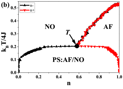
Figure 1: The phase diagrams of the model for $U/4J=2$: (a) $k_{B}T/4J$ vs. $\bar{\mu}/4J$ and (b) $k_{B}T/4J$ vs. $n$ ($L=20$). $\mathbf{T}$ denotes a tricritical point. On panel (a) “heating” and “cooling” label the boundaries obtained by simulation performed with increasing and decreasing temperature, whereas “average” is the average of these two results. They differ if the AF–NO transition is first-order.

We have used the Monte Carlo (MC) simulations to analyze the system. Simulations have been done using Hamiltonian described above on two dimensional square lattice with $N=L\times L$ sites in the grand canonical ensemble, which allows us to obtain e.g. chemical potential dependence of electron concentration curves — $n(\mu)$. The Monte Carlo algorithm used in this analysis consists of three steps: (i) creation, (ii) destruction, and (iii) moving of particle, all of them with appropriate probability $P\sim\exp{\left(\Delta E/(k_{B}T)\right)}$ P2006 ; PK2008 ; MKPR2012 ; MKPR2014 . It is worth noting, that for constant values of concentration a simpler algorithm with only step (iii) — ,,move” would be sufficient. However, addition of the grand canonical parts (creation and destruction) allows one for more detailed analysis in full range of chemical potential and concentration. Unfortunately, addition of chemical potential term in the Hamiltonian prevents us from implementing cluster updates algorithm, so only local updates H1990 are used here. The details of the algorithm used can be found in P2006 ; PK2008 ; MKPR2012 ; MKPR2014 .

The exact ground state ($T=0$) results for this model have been found in the case of a $d=1$ chain MPS2012 ; MPS2013 using the Green function formalism as well as for $2\leq d<+\infty$ case BS1986 ; J1994 . The rigorous results for finite temperatures $T>0$ have been also obtained MPS2013 ; N1 for $d=1$ chain (an absence of long-range order at $T>0$). Within the variational approach (with on-site $U$ term treated exactly and mean field decoupling of intersite term $J$) the model has been analyzed for half-filing ($n=1$) R1975 ; R1979 as well as for arbitrary electron concentration $0\leq n\leq 2$ KKR2010 (these results are rigorous in the limit of infinite dimensions $d\rightarrow+\infty$). Our preliminary Monte Carlo (MC) results have been presented in MKPR2012 ; MKPR2014 for $L=10$ and on-site repulsion: $U/(4J)=1,10$ (corresponding to rather weak and strong coupling, respectively) MKPR2012 as well as for $L=20$ and $U/(4J)=1$ MKPR2014 .

In the present paper we investigate in details the phase diagram and thermodynamic properties of the model for arbitrary electron concentration $n\leq 1$ and arbitrary chemical potential $\bar{\mu}\leq 0$ ($\bar{\mu}=\mu-U/2$) in the whole range of temperatures for $U/(4J)=2$ and $L=20$. In particular, we focus on a behavior of an electron compressibility. The corresponding results for $n>1$ ($\bar{\mu}>0$) are obvious because of the electron-hole symmetry of the model on alternate lattices mentioned previously.

II Results and discussion ($U/(4J)=2$)

Finite temperature phase diagrams for this model were obtained using MC simulations for $U/(4J)=2$ (and $L=20$) as a function of $\bar{\mu}/4J$ and $n$ are presented in Fig. 1(a) and Fig. 1(b), respectively.

The behavior of this system for fixed $\bar{\mu}$ is rather simple (Fig. 1(a)), with both first-order (below $\mathbf{T}$-point) and second-order (above $\mathbf{T}$-point) phase transitions separating non-ordered (NO) and antiferromagnetic (AF) phases with tricirtical point $\mathbf{T}$ located at $k_{B}T/4J=0.205\pm 0.003$, $\bar{\mu}/4J=-1.405\pm 0.007$ ($n\simeq 0.58$). The location of $\mathbf{T}$-point has been determined using hysteresis analysis MKPR2014 . In Fig. 1(a) “heating” and “cooling” label the boundaries obtained by simulation performed with increasing and decreasing temperature whereas “average” is the average of these two results. They differ if the AF–NO transition is first-order. Details of this method can be found in MKPR2014 .

With simulations done for fixed $\bar{\mu}$ and $k_{B}T/4J$ vs. $\bar{\mu}/4J$, it is possible to obtain phase diagrams as a function of $n$ (shown in Fig. 1(b)) by determining electron density above ($n_{-}$) and below ($n_{+}$) the AF–NO phase transition (for fixed $\bar{\mu}$). The first-order AF–NO boundary for fixed $\bar{\mu}$ splits into two boundaries (i.e. PS–AF and PS–NO) for fixed $n$. At sufficiently low temperatures, i.e. below $\mathbf{T}$-point, a phase separated (PS: AF/NO) state occurs. The PS state is a coexistence of two (AF and NO) homogeneous phases. At higher temperatures (i.e. above $\mathbf{T}$-point) the AF–NO transition is second-order one.

An objective indicator of a PS state existence is the evolution of the compressibility $K$ of the system P2006 ; PK2008 . For a system with variable number of particles it can be defined as

$$\frac{1}{K}=n^{2}\left(\frac{\partial\mu}{\partial n}\right)_{T,U,J}.$$ (2)

From this definition it follows that at a fixed $\mu$ the number of particles in an open system can fluctuate freely (precisely, in some define range) when $K\rightarrow\pm\infty$. Such a behavior is connected with an occurrence of the PS states in define range of $n$. At the same constant total free energy of the system the number of domains as well as their distribution can change. Hence, the phase separation states are ,,highly unstable” in that sense that they are subjected to continuous fluctuations of local density (but the total density $n$ is constant).

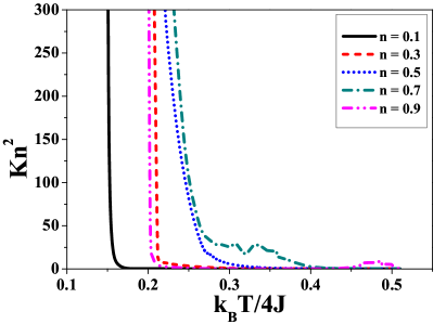
Figure 2: Compressibility $K$ as a function of temperature $T$ for constant values of electron concentration $n$ (as labeled) for $L=20$. For $n>0.58$ there are fluctuations of $K$ associated with second-order AF–NO phase transitions.

Figure 3: A map of compressibility $Kn^{2}$ on $k_{B}T/4J$–$n$ plane (for $L=20$). Solid black curves indicate the phase boundaries derived in Fig. 1(b) plotted for the comparison.

In Fig. 2 the compressibility $Kn^{2}$ is plotted versus temperature $k_{B}T/4J$ for several constant values of $n$. As is clearly seen, close to the boundaries of the PS:AF/NO state occurrence plotted in Fig 1(b), the value of compressibility abruptly increase and $K\rightarrow+\infty$ at transition temperature, indicating an existence of the phase separation state. At higher temperatures and for larger concentrations than those corresponding to the $\mathbf{T}$-point ($n\gtrsim 0.58$) there are compressibility fluctuations related to second order AF–NO phase transition as shown on Fig. 2 at higher temperatures. They are significantly smaller than the fluctuations close to the boundaries below which the PS:AF/NO state occurs.

Fig. 3 presents a map of compressibility on $k_{B}T/4J$–$n$ plane together with the phase boundaries derived in Fig. 1(b) plotted for the comparison. An increase of compressibility close to the second-order AF–NO boundary is clearly seen. The boundary between homogeneous phases and phase separation state is also visible, with the compressibility close to the boundary being at least an order of magnitude greater than those inside the homogeneous phases. As it was said earlier, in the case of phase separation occurrence $K\rightarrow\infty$, so no points are shown inside the region of the PS state occurrence in Fig. 3.

III Final comments

Notice that the results presented are in good qualitative agreement with mean field calculations using variational approach presented in R1979 ; R1975 ; R1973 ; KKR2010 ; MKPR2012 ; K2012 . When comparing these results one should keep in mind differences between these two methods, as the VA is exact only for infinite dimensions $d\rightarrow\infty$. The drawback of Monte Carlo simulations is long thermalization time, which prevents us from obtaining results for the ground state and very low temperatures, as in these conditions electrons have very small probability of escaping local energy minima. Behavior of the model considered in the case of finite band ($t\neq 0$) is very interesting and mostly open problem in the general case MRR1990 ; JM2000 ; DJSZ2004 ; CzR2006 ; DJSTZ2006 ; CzR2006a .

- (1) H. Barz, Materials Research Bulletin 8, 983 (1973). DOI: 10.1016/0025-5408(73)90083-4
- (2) A.K. Rastogi, A. Berton, J. Chaussy, R. Tournier, H. Patel, R. Chevrel, M. Sergent, J. Low Temp. Phys. 52, 539 (1983). DOI: 10.1007/BF00682130
- (3) S. Lamba, A.K. Rastogi, D. Kumar, Phys. Rev. B 56, 3251 (1997). DOI: 10.1103/PhysRevB.56.3251
- (4) E. Berg, E. Fradkin, S.A. Kivelson, J.M. Tranquada, New. J. Phys 11, 115004 (2009). DOI: 10.1088/1367-2630/11/11/115004
- (5) R. Micnas, J. Ranninger, S. Robaszkiewicz, Rev. Mod. Phys. 62, 113 (1990). DOI: 10.1103/RevModPhys.62.113
- (6) G.I. Japaridze, E. Müller–Hartmann, Phys. Rev. B 61, 9019 (2000). DOI: 10.1103/PhysRevB.61.9019
- (7) C. Dziurzik, G.I. Japaridze, A. Schadschneider, J. Zittartz, Eur. Phys. J. B 37, 453 (2004). DOI: 10.1140/epjb/e2004-00081-5
- (8) W.R. Czart, S. Robaszkiewicz, Phys. Status Solidi (b) 243, 151 (2006). DOI: 10.1002/pssb.200562502
- (9) C. Dziurzik, G.I. Japaridze, A. Schadschneider, I. Titvinidze, J. Zittartz, Eur. Phys. J. B 51, 41 (2006). DOI: 10.1140/epjb/e2006-00193-x
- (10) W.R. Czart, S. Robaszkiewicz, Acta Phys. Pol. A 109, 577 (2006);
- (11) [] W.R. Czart, S. Robaszkiewicz, Material Science – Poland 25, 485 (2007).
- (12) G. Pawłowski, Eur. Phys. J. B 53, 471 (2006). DOI: 10.1140/epjb/e2006-00409-1
- (13) G. Pawłowski, T. Kaźmierczak, Solid State Communications 145, 109 (2008). DOI: 10.1016/j.ssc.2007.10.015
- (14) S. Murawski, K. Kapcia, G. Pawłowski, S. Robaszkiewicz, Acta Phys. Pol. A 121, 1035 (2012).
- (15) S. Murawski, K.J. Kapcia, G. Pawłowski, S. Robaszkiewicz, Acta Phys. Pol. A 126, A-110 (2014). DOI: 10.12693/APhysPolA.126.A-110
- (16) D.W. Heermann, Computer Simulation Methods in Theoretical Physics, 2nd Edition, DOI: 10.1007/978-3-642-75448-7 Springer-Verlag, Berlin-Heidelberg 1990
- (17) F. Mancini, E. Plekhanov, G. Sica, Cen. Eur. J. Phys. 10, 609 (2012). DOI: 10.2478/s11534-012-0017-z
- (18) F. Mancini, E. Plekhanov, G. Sica, Eur. Phys. J. B 86, 224 (2013). DOI: 10.1140/epjb/e2013-40046-y
- (19) U. Brandt, J. Stolze, Z. Phys. B 62. 433 (1986). DOI: 10.1007/BF01303574
- (20) J. Jędrzejewski, Physica A 205, 702 (1994). DOI: 10.1016/0378-4371(94)90231-3
- (21) K.J. Kapcia, W. Kłobus, S. Robaszkiewicz, Acta Phys. Pol. A 127, 284 (2015). DOI: 10.12693/APhysPolA.127.284
- (22) S. Robaszkiewicz, Acta Phys. Pol. A 55, 453 (1979).
- (23) S. Robaszkiewicz, Phys. Status Solidi (b) 70, K51 (1975). DOI: 10.1002/pssb.2220700156
- (24) W. Kłobus, K. Kapcia, S. Robaszkiewicz, Acta Phys. Pol. A 118, 353 (2010);
- (25) [] K. Kapcia, W. Kłobus, S. Robaszkiewicz, Acta Phys. Pol. A 121, 1032 (2012).
- (26) S. Robaszkiewicz, Phys. Status Solidi (b) 59, K63 (1973). DOI: 10.1002/pssb.2220590155
- (27) K. Kapcia, Acta Phys. Pol. A 121, 733 (2012);
- (28) [] K.J. Kapcia, Acta Phys. Pol. A 127, 281 (2015); DOI: 10.12693/APhysPolA.127.281
- (29) [] K.J. Kapcia, J. Supercond. Nov. Magn. 28, 1289 (2015). DOI: 10.1007/s10948-014-2906-4