Two-Component Structure in the Entanglement Spectrum of Highly Excited States

Abstract

We study the entanglement spectrum of highly excited eigenstates of two known models that exhibit a many-body localization transition, namely the one-dimensional random-field Heisenberg model and the quantum random energy model. Our results indicate that the entanglement spectrum shows a “two-component” structure: a universal part that is associated with random matrix theory, and a nonuniversal part that is model dependent. The nonuniversal part manifests the deviation of the highly excited eigenstate from a true random state even in the thermalized phase where the eigenstate thermalization hypothesis holds. The fraction of the spectrum containing the universal part decreases as one approaches the critical point and vanishes in the localized phase in the thermodynamic limit. We use the universal part fraction to construct an order parameter for measuring the degree of randomness of a generic highly excited state, which is also a promising candidate for studying the many-body localization transition. Two toy models based on Rokhsar-Kivelson type wave functions are constructed and their entanglement spectra are shown to exhibit the same structure.

Introduction.–Quantum entanglement, a topic of much importance in quantum information theory, has also gained relevance in quantum many-body physics in the past few years AmicoRMP ; EisertRMP . In particular, the entanglement entropy provides a wealth of information about physical states, including novel ways to classify states of matter that do not have a local order parameter wen . However, it has been realized only recently in various physical contexts that the entanglement entropy is not enough to fully characterize a generic quantum state. For example, the quantum complexity corresponding to the geometric structure of black holes cannot be fully encoded just by the entanglement entropy Susskind . One natural step beyond the amount of entanglement is the specific pattern of entanglement, i.e., the entanglement spectrum. A recent result that motivates this direction is the relationship between irreversibility and entanglement spectrum statistics in quantum circuits CHM ; Shaffer . It was shown that irreversible states display Wigner-Dyson statistics in the level spacing of entanglement eigenvalues, while reversible states show a deviation from Wigner-Dyson distributed entanglement levels and can be efficiently disentangled.

Are there universal features in the entanglement spectrum of a generic eigenstate of a quantum Hamiltonian? Highly excited eigenstates of a generic quantum Hamiltonian are believed to satisfy the “eigenstate thermalization hypothesis” (ETH) Deutsch ; Srednicki ; Rigol , which states that the expectation value $\langle\psi_{\alpha}|\hat{O}|\psi_{\alpha}\rangle$ of a few-body observable $\hat{O}$ in an energy eigenstate $|\psi_{\alpha}\rangle$ of the Hamiltonian with energy $E_{\alpha}$ equals the microcanonical average at the mean energy $E_{\alpha}$. So one could as well ask the following question: What is the structure of the entanglement spectrum of highly excited eigenstates of a thermalized system? Here we find a quandary. Completely random states are generically not physical, namely, they cannot be the eigenstates of Hamiltonians with local interactions. For the ETH to be a physical scenario for thermalization, highly excited eigenstates of physical local Hamiltonians cannot always be completely random, yet they have to contain enough entropy. Deviations from a completely random state can be quantified by the entanglement entropy, more precisely by the amount that it deviates from the maximal entropy in the subsystem, derived by Page, which we will refer to as the Page entropy hereafter Page . But are there features that cannot be captured by the entanglement entropy alone? Can one identify remnants of randomness in the full entanglement spectrum? What about in states that violate the ETH?

In this Letter, we address the above questions using as a case study the problem of many-body localization (MBL) Nandkishore ; oganesyan07 ; Pal_Huse ; Moore ; Abanin . We study two known models that were shown to exhibit a MBL transition, namely, the Heisenberg spin model with random fields, and the quantum random energy model (QREM) Kurchan ; QREM ; QREM2 . In the delocalized phase, high-energy eigenstates are thermalized according to the ETH. The deviation from completely random states manifests itself in a “two-component” structure in the entanglement spectrum: a universal part that corresponds to random matrix theoryMehta , and a nonuniversal part that is model dependent. We show that the universal part fraction decreases as one approaches the transition point and vanishes in the localized phase in the thermodynamic limit. We therefore propose an order parameter that is able to measure the degree of randomness of a generic highly excited state and capture the many-body localization-delocalization transition based on the entanglement spectrum, and show that it gives predictions consistent with previous results. We further construct two toy models in terms of Rokhsar-Kivelson- (RK) type wavefunctions RK ; RK_2 and the same structure in the entanglement spectra is observed.

Heisenberg spin chain.–A well-studied model that shows a MBL transition is the isotropic Heisenberg spin-1/2 chain with random fields along a fixed direction,

$$\mathcal{H}=\sum_{i=1}^{L}\left(h_{i}\,S_{i}^{z}+J\,\vec{S}_{i}\cdot\vec{S}_{i+1}+\Gamma S_{i}^{x}\right),$$ (1)

where the random fields $h_{i}$ are independent random variables at each site, drawn from a uniform distribution in the interval $[-h,h]$. $\Gamma$ is a uniform transverse field along the $x$ direction, which breaks total $S_{z}$ conservation. We assume periodic boundary condition and set the coupling $J=1$ and $\Gamma=0.1$. In the absence of the transverse field $\Gamma$, previous work located the critical point at $h=h_{c}\approx 3.5$ in the $S_{z}=0$ sector Pal_Huse ; Heisenberg ; Serbyn . We consider two different regimes by varying the disorder strength parameter $h$: (i) within the thermalized phase ($h<h_{c}$), and (ii) in the localized phase ($h>h_{c}$). In each regime, we focus on eigenstates of Hamiltonian (1) at the middle of the spectrum, namely, on highly excited states.

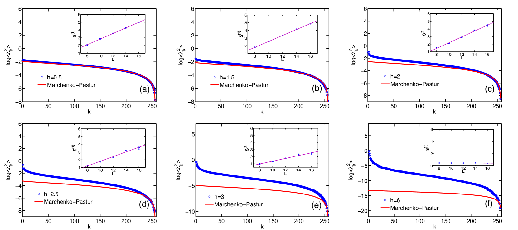
Figure 1: (Color online) Average entanglement spectrum of highly excited eigenstates for a system of size $L=16$, averaged over 10 realizations of disorder (plotted in logarithmic scale). Panels a–f show the spectrum for $h=0.5,1.5,2,2.5,3$ and $6$, respectively. The solid lines correspond to the spectrum of a completely random state (derived from a Marchenko-Pastur distribution), and is shown for reference. Insets: scaling of the average entanglement entropy $S^{(1)}$ with system size.

We consider a bipartition of the system into subsystems $A$ and $B$ of equal size ($L/2$ sites each). For a generic eigenstate $|\psi\rangle=\sum_{\bm{\sigma}}\psi(\bm{\sigma})|\bm{\sigma}\rangle$, where $\bm{\sigma}\equiv\sigma_{1}\sigma_{2}\dots\sigma_{L}$ labels the $2^{L}$ possible spin configurations of the system, we cast the wave function as $\psi(\bm{\sigma})\equiv\psi(\bm{\sigma}_{A}\,\bm{\sigma}_{B})$, where $\bm{\sigma}_{A}\equiv\sigma_{1}\dots\sigma_{L/2}$ and $\bm{\sigma}_{B}\equiv\sigma_{L/2+1}\dots\sigma_{L}$. The entanglement spectrum is obtained from the eigenvalues of the reduced density matrices $\rho_{A}={\rm tr}_{B}|\psi\rangle\langle\psi|$ and $\rho_{B}={\rm tr}_{A}|\psi\rangle\langle\psi|$: $\{p_{k}=\lambda_{k}^{2}\},k=1,\ldots 2^{L/2}$. In this work, we are primarily concerned with the density of states and level statistics of the $\{\lambda_{k}\}$ for highly excited eigenstates for different strengths of disorder. For each value of $h$ analyzed, the spectra were averaged over 10 realizations of disorder for $L=16$, and 100 realizations for $L=14$. For each spectrum, the eigenstate with energy closest to zero was obtained by a Lanczos projection anders . This eigenstate corresponds to a highly excited state.

Thermalized phase.–We start by considering the weakly disordered case, $h\ll h_{c}$. Only a small amount of disorder is necessary to break the integrability of the clean Hamiltonian. However, conservation of the total $S_{z}$ also plays a crucial role in making eigenstates completely random. A small transverse field $\Gamma$ is applied to break this conservation without substantially altering the many-body localization transition. In this regime, we find that the entanglement spectrum of the highly excited state with eigenenergy near zero is close to that of a completely random quantum state, as shown in Fig. 1(a) for systems of size $L=16$ and $h=0.5$. The entanglement spectrum follows closely a Marchenko-Pastur distribution (with proper normalization), which describes the asymptotic average density of eigenvalues of a Wishart matrix Marchenko-Pastur ; Znidaric . (The expression for the entanglement spectral density for the random state is presented in the Supplemental MaterialSM .) One can also check that, in this regime, the von Neumann entanglement entropy $S^{(1)}=-\sum_{k}p_{k}\ln p_{k}$ is in good agreement with the Page entropy for random states: $S_{m,n}=\sum_{k=n+1}^{mn}\frac{1}{k}-\frac{m-1}{2n}\approx{\rm ln}(m)-\frac{m}{2n}$, where $m$ and $n$ are the Hilbert space dimensions of subsystem $A$ and $B$, respectively Page . For example, our computed average entropy for 16 sites is $\langle S^{(1)}\rangle=4.9719\pm 0.0015$, while the corresponding Page entropy is $S_{\rm Page}=5.0452$.

As the disorder strength is increased, but still $h<h_{c}$, the system remains in the thermalized phase where it is supposed to obey the ETH and yield volume-law scaling of the entanglement entropy with system sizes Deutsch_Li_Sharma , which is verified in the insets of Figs. 1(a) to 1(e). However, in spite of the volume-law scaling of the entanglement entropy and the thermalization of eigenstates, the entanglement entropy is much lower than the Page entropy. This indicates that the pattern of entanglement must have changed, which is manifest in the spectra shown in Figs. 1(b) to 1(e). The entanglement spectrum shows a striking “two-component” structure: (i) a universal tail in agreement with random matrix theory, and (ii) a nonuniversal part. The non-universal part dominates the weights in the spectrum (large $\lambda_{k}$ values), resulting in low entanglement entropy, as it decays much faster than the universal part. Therefore, we find that although thermalized states are not necessarily random states, they partially retain a component that is reminiscent of a random state: the entanglement spectrum follows the Marchenko-Pastur level density distribution. In addition, the universal part of the entanglement spectrum follows a Wigner-Dyson distribution of level spacings (see the Supplemental MaterialSM ).

Localized phase.–In this regime, the entanglement entropy exhibits an area-law scaling with the system size [see inset of Fig. 1(f)], which in one spatial dimension implies a constant entropy and, at most, weakly logarithmic corrections, in accordance with Ref. Bauer .

The entanglement spectrum in the localized regime, depicted in Fig. 1(f) for $h=6$, shows a different scenario from that in the thermalized phase: the universal part of the spectrum disappears completely, leaving only the nonuniversal part characterized by its fast decay rate.

QREM.–The QREM describes $L$ spins in a transverse field $\Gamma$ with the following Hamiltonian:

$$\mathcal{H}=E(\{\sigma^{z}\})+\Gamma\sum_{i=1}^{L}\sigma_{i}^{x}$$ (2)

where $E(\{\sigma^{z}\})$ is the classical REM term that takes independent values from a Gaussian distribution of zero mean and variance $L/2$ Derrida . This model was first studied in the context of a mean-field spin glass, and was shown to exhibit a first-order quantum phase transition as a function of $\Gamma$ Kurchan . More recently, it was further demonstrated to have a MBL transition when viewed as a closed quantum system QREM . Numerical and analytical arguments show that the transition happens at an energy density $|\epsilon|=\Gamma$ in the microcanonical ensemble. Since there is no support for the many-body localized phase at energy density $\epsilon=0$, we examine the eigenstates with energy density closest to $\epsilon=0.5$ instead, and study the entanglement spectrum as $\Gamma$ is tuned. The two-component structure and its evolution as a function of $\Gamma$ similar to Fig. 1 are again observed (see the Supplemental MaterialSM ).

An order parameter.–The above picture unveils a new aspect of the MBL transition. The two parts of the entanglement spectrum of a highly excited state clearly evolve as the disorder strength $h$ is increased, namely, the universal part shrinks and the nonuniversal part grows. This fact suggests that one could use the fraction of each component as an order parameter.

Figures 1(a) to 1(e) indicate an $h$ dependent value $k_{h}$ that separates the nonuniversal ($k\leq k_{h}$) from the universal ($k>k_{h}$) parts of the rank-ordered entanglement levels (see the Supplemental Material SM for the protocol for determining $k_{h}$). One can thus define the partial Rényi entropies

$$S_{\leq}^{(q)}=\frac{1}{1-q}\ln\sum_{k\leq k_{h}}\;p_{k}^{q}\;,$$ (3)

with $q\geq 0$. Because the universal part of the spectrum is where the eigenvalues with low entanglement reside, this part of the spectrum is obscured by any measure that relies on the eigenvalues as weights. A good measure of the fraction of the two components that does not depend on these weights is given by the $q=0$ Rényi entropy, which simply measures the ranks: $S_{\leq}^{(0)}=\ln k_{h}$. Therefore, an order parameter that measures the fraction of the universal component is

$${\cal O}_{\rm MBL}=1-\frac{S_{\leq}^{(0)}}{S^{(0)}}=1-\frac{\log_{2}k_{h}}{{L/2}}\;.$$ (4)

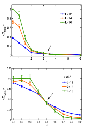
Figure 2: (Color online) The order parameter defined as the fraction of the universal component in the full entanglement spectrum for the Heisenberg spin model (upper panel) and the QREM (lower panel).

Figure 2 shows the order parameter as defined above for the Heisenberg spin model and the QREM, respectively. For the QREM, all curves at different system sizes cross at $\Gamma_{c}\approx 0.5$, in excellent agreement with Ref. QREM . We have also looked at energy density $\epsilon=0.3$, and the curves cross at $\Gamma_{c}\approx 0.25$, giving the same numerical prediction as in Refs. QREM and QREM2 (plot shown in the Supplemental Material SM ). For the random-field Heisenberg model, however, the fact that the transition happens at the point where the order parameter is nearly zero makes it harder to accurately locate the critical point using our order parameter. We see from Fig. 2 that the curves cross at $h_{c}\approx 3.3$, which is also consistent with previous studies. This indicates that, by considering the full entanglement spectrum at high energies, our order parameter reveals a novel property that is promising for studying the MBL transition.

We remark that, although the MBL transition can also be captured by the scaling property of the entanglement entropy, our order parameter seems to be applicable even for models with nonlocal interactions, which could obscure the connection between the volume-to-area law transition of the entropy and the MBL transition.

Toy models.–we construct two RK-type model wave functions that are shown to have (i) the two-component structure in their entanglement spectra, and (ii) a phase transition as a function of the tuning parameter. The wave functions take the following form:

$$|\Psi\rangle=\frac{1}{\sqrt{\mathcal{Z}}}\sum_{{\bm{\sigma}}}s_{{\bm{\sigma}}}{\rm e}^{-\frac{\beta}{2}E({\bm{\sigma}})}|{\bm{\sigma}}\rangle,$$ (5)

where $E({\bm{\sigma}})$ is the energy for the classical configuration ${\bm{\sigma}}$ and $\mathcal{Z}$ is the corresponding partition function of the classical statistical system RK_2 . $s_{\bm{\sigma}}$ is a random sign for each configuration, such that the wave function represents a highly excited state. We consider the following two cases: (i) $E({\bm{\sigma}})=E_{{\rm REM}}({\bm{\sigma}})$, and (ii) $E({\bm{\sigma}})=-\frac{J}{L}\sum_{i<j}\sigma_{i}^{z}\sigma_{j}^{z}$. In the first case, the energy is taken to be that of the REM, while in the second case the energy is that of an infinite-range uniform ferromagnetic interaction.

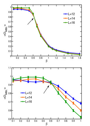
Figure 3: (Color online) The order parameter for the random-sign RK-type wave functions. Upper panel: $E({\bm{\sigma}})=E_{{\rm REM}}({\bm{\sigma}})$. Lower panel: $E({\bm{\sigma}})=-\frac{J}{L}\sum_{i<j}\sigma_{i}^{z}\sigma_{j}^{z}$, with $J=1$.

In the small $\beta$ regime, the above RK-type wave functions are close to completely random states; upon increasing $\beta$, the wave functions are pushed towards product states and start to deviate from completely random states. Therefore, the tuning parameter $\beta$ here plays the role of the “disorder strength”. Indeed, we find the same two-component structure in the entanglement spectrum (see the Supplemental Material SM ), and the order parameter is shown in Fig. 3. The REM case was recently studied by Chen et al. where the MBL transition was obtained numerically using other measures Fradkin . Here we clearly see that, in both cases, the curves cross at some critical $\beta$, indicating the existence of a similar phase transition.

Summary and discussion.–The details of the structure of the entanglement spectrum, especially the universal part at the tails of the spectrum, have long been overlooked. The main focus has been primarily on the dominating nonuniversal component, and the universal tail has thus far been discarded. For example, in the density matrix renormalization group DMRG and tensor network methods MPS , the density matrix is truncated to avoid uncontrolled growth of its dimensions. While this procedure is certainly justified when the purpose is to obtain ground state properties, it discards important information about the behavior of the system at higher energy states. In this Letter we showed that the full entanglement spectrum, directly computable from the wave function, provides information that is often invisible in the entanglement entropy alone.

On the other hand, much has been known about random quantum states, e.g., the Page entropy and volume-law scaling entropy. Nevertheless, the Page entropy is often an overestimate of the actual entanglement entropy computed from generic quantum states. Therefore, a natural question that arises is as follows: How random does a given quantum state look? In this Letter, we show that a generic quantum state that satisfies ETH does not necessarily mean a completely random state. We present an order parameter to quantify the degree of randomness by using information about the full entanglement spectrum. In the context of MBL, our order parameter is able to locate the critical point, consistent with previous results. Our work may provide a novel way of studying MBL, and may shed new light on the understanding many-body systems at the level of wave functions.

Z.-C.Y. is indebted to Bernardo Zubillaga, Alexandre Day, Shenxiu Liu, and Yi-Zhuang You for generous help and useful discussions. We thank Christopher Laumann for useful comments. This work was supported in part by DOE Grant No. DEF-06ER46316 (C.C.), by NSF Grant No. CCF 1117241 (E. R. M.), by National Basic Research Program of China Grants No. 2011CBA00300 and No. 2011CBA00301, and by National Natural Science Foundation of China Grant No. 61361136003 (A.H.)

I Supplemental Material

II Marchenko-Pastur distribution and random states

The Marchenko-Pastur distribution describes the asymptotic (large-$N$) average density of eigenvalues of an $N\times N$ matrix of the form $Y=XX^{\dagger}$, known as a Wishart matrix, where $X$ is a $N\times M$ random rectangular matrix with independent but identically distributed entries Marchenko-Pastur . Let $\sigma^{2}$ be the variance of the entries in $X$. When $N=M\rightarrow\infty$, the Marchenko-Pastur distribution takes the form

$${\cal D}(p)=\left\langle\frac{1}{N}\sum_{k=1}^{N}\delta(p-p_{k})\right\rangle_{N\rightarrow\infty}=\frac{2}{\pi p_{\rm max}}\sqrt{\frac{p_{\rm max}}{p}-1},$$ (6)

where $\{p_{k}\}$ are the eigenvalues of $Y$, $0\leq p\leq p_{\rm max}$ and $p_{\rm max}=2\sigma^{2}$. From this distribution we can obtain the average number function associated to the eigenvalues of $Y$. Let $p_{1}\geq p_{2}\geq\cdots\geq p_{N}$ and $\eta_{k}=k/N$. Then,

$$\eta(p) = 1-\left\langle\frac{1}{N}\sum_{k=1}^{N}\theta(p-p_{k})\right\rangle_{N\rightarrow\infty}$$ (7)

$$= \left[1-\int_{0}^{p}dp^{\prime}\,{\cal D}(p^{\prime})\right]$$ (8)

$$= \int_{p}^{p_{\rm max}}dp^{\prime}\,{\cal D}(p^{\prime})$$ (9)

$$= 1-\frac{2}{\pi}\left[u\sqrt{1-u^{2}}+\mbox{arcsin}(u)\right]_{u=\sqrt{p/p_{\rm max}}}.$$ (10)

Thus, introducting the rescaled variable $x=\sqrt{p/p_{\rm max}}$, we find

$$\eta(x)=1-\frac{2}{\pi}\left[x\sqrt{1-x^{2}}+\mbox{arcsin}(x)\right].$$ (11)

It is straightforward to relate the average number function derived from the Marchenko-Pastur distribution with that obtained from the entanglement spectrum of a bipartitioned random vector. Let $\psi(x_{A},x_{B})$ be the wavefunction of the bipartite system. Then, the reduced density matrix is given by

$$\rho_{A}(x_{A},x_{A}^{\prime})=\sum_{x_{B}}\psi(x_{A},x_{B})\,\psi^{\ast}(x_{A}^{\prime},x_{B}).$$ (12)

We can see that, for completely random wavefunctions, the reduced density matrix is a random Wishart matrix and therefore its eigenvalues should follow a Marchenko-Pastur distributionZnidaric . Thus, we expect the average number function to provide an accurate description of the average spectrum.

Let $\{p_{k}\}$, $k=1,\ldots,d$, be the set of eigenvalues of $\rho_{A}$ in decreasing order, with $p_{k}\geq 0$, $\sum_{k=1}^{d}p_{k}=1$, and $d\leq 2^{L/2}$. It is straightforward to relate the eigenvalues $\{p_{k}\}$ to the singular values $\{\lambda_{k}\}$ resulting from the Schmidt decomposition of the bipartite wavefunction,

$$\psi(x_{A},x_{B})=\sum_{k=1}^{d}\lambda_{k}\,\phi_{A}^{(k)}(x_{A})\,\phi_{B}^{(k)}(x_{B}),$$ (13)

by simply setting $p_{k}=\lambda_{k}^{2}$ (notice that $\lambda_{k}\geq 0$), where $\phi_{A}^{(k)}(x_{A})$ and $\phi_{B}^{(k)}(x_{B})$ are the left-singular and right-singular vectors, respectively. For the purpose of comparing the average spectra to Eq. (11), it is necessary to rescale the singular values and their indices as follows:

$$p_{k}=\frac{4}{d}x^{2}(\eta_{k})$$ (14)

where $x(\eta)$ is the inverse function of $\eta(x)$. The prefactor is chosen to guarantee the normalization of $p_{k}$:

$$\sum_{k=1}^{d}p_{k} \rightarrow 4\int_{0}^{1}{\rm d}\eta\,x^{2}(\eta)$$ (15)

$$= \frac{16}{\pi}\int_{0}^{1}{\rm d}x\,x^{2}\sqrt{1-x^{2}}$$

$$= 1.$$

We tested this formulation by plotting the numerical results for $p_{k}$ obtained from a random state against the analytical expression in Eq. (11). Figure 4 shows $\eta_{k}=\frac{k}{d}$ versus $x_{k}=\frac{1}{2}\sqrt{p_{k}d}$. There is very good agreement with the analytical prediction.

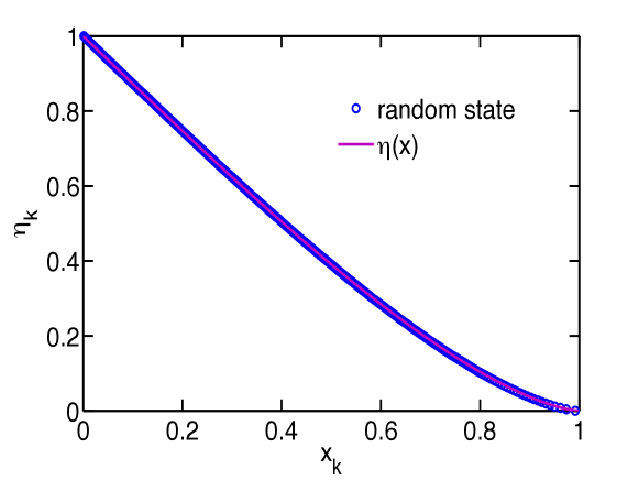
Figure 4: Average entanglement pectrum of completely random wavefunction ($L=16$, 100 realizations used).

Notice that in the cases considered in the main text, the random part of the entanglement spectrum alone is not normalized. However, by plotting ${\rm log}\lambda_{k}$ versus $k$, the missing normalization factor only amounts to a trivial shift of the entire spectrum.

III Level spacing statistics

We studied the statistics of the entanglement spectrum by looking at the level spacing distribution in the set $\{\lambda_{k}\}$. To avoid having to perform spectral unfolding, we chose to evaluate the distribution of ratios of adjacent level spacings oganesyan07 : $r_{k}=(\lambda_{k+1}-\lambda_{k})/(\lambda_{k}-\lambda_{k-1})$. Accurate surmises exist for the distribution of these ratios in the case of Gaussian ensembles atas13 . They are given by

$$P_{\rm WD}(r)=\frac{1}{Z}\frac{(r+r^{2})^{\beta}}{(1+r+r^{2})^{1+3\beta/2}},$$ (16)

where $Z=\frac{8}{27}$ for the Gaussian Orthogonal Ensemble (GOE) with $\beta=1$, and $Z=\frac{4}{81}\frac{\pi}{\sqrt{3}}$ for the Gaussian Unitary Ensemble (GUE) with $\beta=2$. The corresponding distribution for the Poisson distributed spectrum is given by the exact form

$$P_{\rm Poisson}=\frac{1}{(1+r)^{2}}.$$ (17)

Notice that for the Gaussian ensembles, level repulsion manifests itself in the asymptotic behavior $P(r\rightarrow 0)\sim r^{\beta}$, which is absent in the case of Poisson statistics.

Results are shown in Fig. 5 for disordered Heisenberg chains with $L=16$ and 100 disorder realizations. A completely random real state follows a GOE statistics. The universal part of the spectrum at $h=0.5$ also follows a GOE distribution.

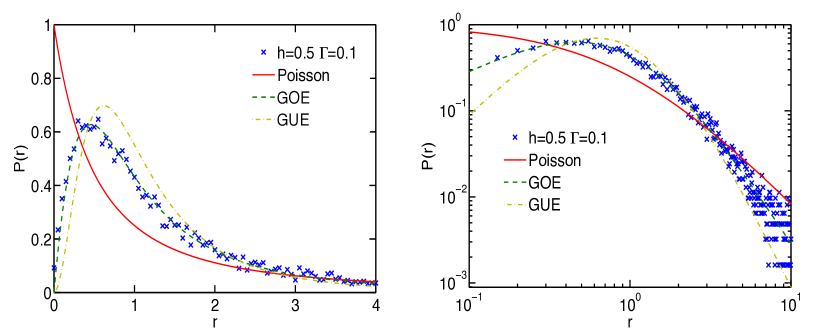
Figure 5: Left panel: Distribution of the ratios of consecutive spacings for the entanglement spectrum of Heisenberg spin chains with disorder parameter $h=0.5$ and transverse field $\Gamma=0.1$ (crosses). Right panel: the same data in a logarithmic scale. $L=16$ and 500 realizations used.

IV Protocol for determining $k_{h}$

The definition of the order parameter in this Letter required a protocol for determining the point $k_{h}$ which separates the non-universal part ($k\leq k_{h}$) from the universal ($k>k_{h}$) part of the rank-ordered entanglement levels. We use the following protocol: we took the spectrum obtained from each random state considered and multiply it by a factor $s$ such that the rescaled smallest singular value coincided in value with that obtained from a completely random state. Then we swept through the spectrum, starting from the tail, and computed the relative deviation from the completely random state prediction, until it exceeded a certain amount. That is, until

$$\frac{(\lambda_{k})^{2}-s(\lambda_{k}^{MP})^{2}}{s(\lambda_{k}^{MP})^{2}}>\epsilon,$$ (18)

where $\epsilon$ is a number of order 1. In our case, we set $\epsilon=1$.

However, we would like to point out one subtlety of this methodology. In cases where the universal component of the spectrum almost vanishes near the transition, it is hard to accurately locate the critical point. That is because the last few points at the tail of the spectrum show large sample-to-sample fluctuations, and our protocol requires strictly matching a single point close to the tail. Therefore, $k_{h}$ can be very sensitive to our choice of the matching point and can even yield incorrect predictions under finite-size scaling. On the other hand, we find that in cases such as the QREM, where there is still a large fraction of the universal component at the transition, this methodology is not very sensitive to the choice of matching point. For the Heisenberg model, we locate the critical point $k_{h}$ by choosing the matching point away from the tail end, thus effectively discarding the smallest eigenvalues. For example, for $L=16$ we discarded the last 16 eigenvalues. In order to demonstrate that this does not lead to a sizable errors in determining the MBL critical point, we also computed the the order parameter directly from the averaged entanglement spectrum, where the fluctuations are smoothened out (Fig. 6). The critical point found this way is very close to the one we show in the main text. We believe that the result can be further improved if more realizations are include in the averaring, which we hope to attempt in the future.

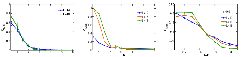
Figure 6: Left: Results obtained when the matching point is chosen too close to the last eigenvalue for each entanglement spectrum, yielding a wrong transition point under finite-size scaling. Middle: the order parameter computed from the averaged entanglement spectrum of the random-field Heisenberg model, where fluctuations are smoothened out and not many small eigenvalues need to be eliminated. Right: the order parameter computed from the average entanglement spectrum of the QREM. One can see that in this case our approach is robust and the result is very close to that shown in the main text.

V Entanglement spectra for QREM and RK-type toy models

In this section, we present in Fig. 7 through Fig. 9 the entanglement spectra for the QREM and two RK-type toy models that were discussed in the main text.

Figure 7: Averaged entanglement spectrum of eigenstates with energy density $\epsilon=0.5$, for the QREM. The system size $L=16$, and $\Gamma=0.9,\ 0.6,\ 0.4$, and 0.2, averaging over 10 realizations of disorder.

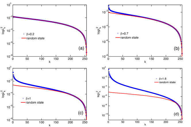
Figure 8: Averaged entanglement spectrum of the RK-type wavefunction, with $E({\bm{\sigma}})=E_{{\rm REM}}({\bm{\sigma}})$. The system size $L=16$, and $\beta=0.2,\ 0.7,\ 1$, and 1.8, averaging over 100 realizations of disorder.

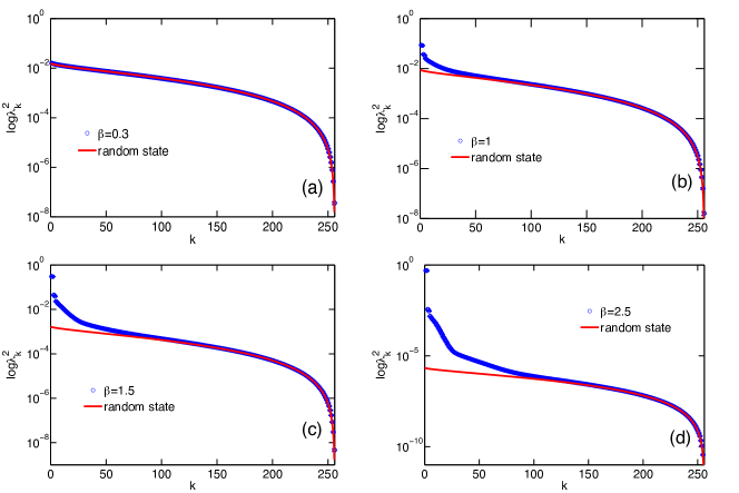
Figure 9: Averaged entanglement spectrum of the RK-type wavefunction, with $E({\bm{\sigma}})=-\frac{J}{L}\sum_{i<j}\sigma_{i}^{z}\sigma_{j}^{z}$. The system size $L=16$, and $\beta=0.3,\ 1,\ 1.5$, and 2.5, averaging over 100 realizations of random sign.

We clearly see the following: (1) the two-component structure shows up in all three cases; (2) the same evolution behavior as explained in the main text happens here as well. Namely, the universal fraction shrinks as one increases the strength of disorder, thereby pushing the states further away from completely random states.

We also show the order parameter for the QREM at energy density $\epsilon=0.3$, which is different from the one shown in the main text. We clearly see from Fig. 10 that the curves for different system sizes cross at around $\Gamma_{c}\approx 0.25$, which is again in excellent agreement with previous known results.

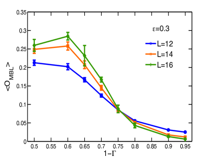
Figure 10: The order parameter for QREM with target energy density $\epsilon=0.3$.

VI Randomness versus non-randomness: another toy model

In this section, we view the emergence of the non-universal component in the entanglement spectrum from a different perspective: the degree of randomness in the wavefunctions. The physical intuition can be understood as follows. A completely random state is supposed to yield a Marchenko-Pastur distribution in its entanglement spectrum, i.e. only the universal component exits. This implies that for states whose entanglement spectra deviate from Marchenko-Pastur distribution, they cannot be completely random. Therefore we construct another toy model which captures this feature, by borrowing ideas from spin glasses.

First let us start with a truly random (real) wavefunction that we denote by $\Psi_{\rm REM}({\bm{\sigma}})={\rm sgn}(E_{\rm REM})$, where ${\rm sgn}(x)$ is the sign function and $E_{\rm REM}$ are identically independently distributed with probability $P(E_{\rm REM})=\frac{1}{\sqrt{\pi L}}{\rm e}^{-E_{\rm REM}^{2}/L}$, with $L$ being the number of spins. The wavefunction $\Psi_{{\rm REM}}$ is, by construction, random. The subscript REM is used to draw an analogy to the Random Energy Model (REM) in spin glass systems16.

Next, we note that the REM is a limiting case of a spin glass with $p$-spin interactions as $p\rightarrow\infty$, which eliminates correlations between configurations. So we can take a step back and consider the following “less random” Sherrington-Kirkpatrick (SK) spin glass model with infinite-range two-spin interactions SK , and construct the following wavefunction:

$$\Psi_{\rm SK}(\bm{\sigma})={\rm sgn}\left(E_{\rm SK}({\bm{\sigma}})\right)={\rm sgn}\left(\sum_{i<j}J_{ij}\;\sigma_{i}\,\sigma_{j}\right),$$ (19)

where the $J_{ij}$ are drawn from uniform distribution in the interval $[-1,1]$. The amplitudes computed from the SK-like model are obviously not as random as in the REM-like one; there are only $L(L-1)/2$ independent random $J_{ij}$’s in the former as opposed to $2^{L}$ independent random amplitudes in the latter. Nevertheless, the amplitudes of $\Psi_{\rm SK}$ do inherit some randomness from the $J_{ij}$, and the energy distribution of the SK-like model also follows accurately a Gaussian distribution for any one given $\bm{\sigma}$, similarly to those in the REM-like model. But the correlations between the amplitudes for different $\bm{\sigma}$ exist in the case of the SK-like model, and these correlations are manifest in the entanglement spectrum computed from $\Psi_{\rm SK}$, as shown in the left panel of Fig. 11.

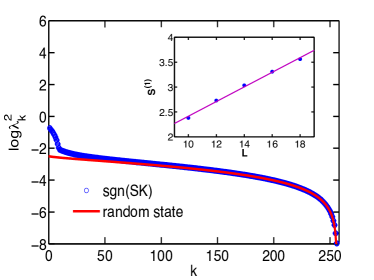
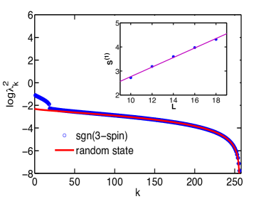
Figure 11: (Color online) Entanglement spectrum of: $\Psi_{\rm SK}$ (left) and $\Psi_{{\rm 3-spin}}({\bm{\sigma}})$ (right), for a system of size $L=16$, averaged over 500 realizations of disorder. The order parameter as defined in Eq. (3) is: $\langle{\mathcal{O}}\rangle=0.3888\pm 0.0067$, with a threshold $k\approx 30$ for $\Psi_{\rm SK}$; and $\langle{\mathcal{O}}\rangle=0.4279\pm 0.0060$, with a threshold $k\approx 24$ for $\Psi_{{\rm 3-spin}}({\bm{\sigma}})$. The insets show the volume-law scaling of the von Neumann entanglement entropy.

The entanglement entropy follows a volume-law scaling (see inset of Fig. 11) and, again, we see the emergence of a two-component structure in the spectrum. The universal part agrees with RMT. The non-universal part is different from that found for the high energy eigenstates of a disordered Heisenberg spin chain, reflecting its non-universal, model dependent nature. Yet, this component is still characterized by its fast decay rate. The toy model shows that non randomness can be present in a generic quantum state when there are correlations between components of the wavefunction. The entanglement spectrum captures the non randomness and its structure can be well described by a two-component picture.

Another interesting manifestation of the mixing between universal and non-universal components in the SK wavefunction is revealed by employing a color map. In Fig. 12 we show the amplitude of the wavefunction $\Psi_{\rm SK}(\bm{\sigma}_{A},\bm{\sigma}_{B})$ plotted in a $\bm{\sigma}_{A}\times\bm{\sigma}_{B}$ grid, and compared it to the amplitude of a REM wavefunction. The existence of a structure, similar to wefts in a tapestry, is clearly visible for the $\Psi_{\rm SK}$ wavefunction, but completely absent for the REM wavefunction.

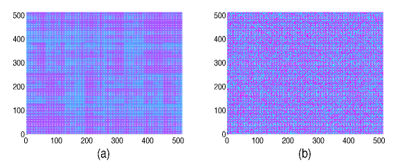
Figure 12: (Color online) Color map of the matrix $\Psi(\bm{\sigma}_{A},\bm{\sigma}_{B})$ for typical realizations of the (a) SK and (b) REM wavefunctions ($L=18$).

One can further consider wavefunctions built with three-spin interactions,

$$\Psi_{{\rm 3-spin}}({\bm{\sigma}})={\rm sgn}\left(\sum_{i<j<k}J_{ijk}\,\sigma_{i}\,\sigma_{j}\,\sigma_{k}\right),$$ (20)

where the $J_{ijk}$ are drawn from a uniform distribution in the interval $[-1,1]$. As shown in the right panel of Fig. 11, the spectrum again shows a two-component structure, very similar to the cases discussed in the main text.

References

- (1) L. Amico, R. Fazio, A. Osterloh, and V. Vlatko, Rev. Mod. Phys. 80, 517 (2008).
- (2) J. Eisert, M. Cramer, and M. B. Plenio, Rev. Mod. Phys. 82, 277 (2010).
- (3) X.G. Wen and Q. Niu, Phys. Rev. B 41, 9377 (1990); X.G. Wen, Phys. Rev. Lett. 90, 016803 (2003); Phys. Lett. A 300, 175 (2002); M. Levin and X. G. Wen, Phys. Rev. Lett. 96, 110405 (2006); A. Kitaev and J. Preskill, Phys. Rev. Lett. 96, 110404 (2006); X.-G. Wen, Quantum Field Theory of Many-Body Systems (Oxford Press, New York, 2004).
- (4) L. Susskind, arXiv:1411.0690.
- (5) C. Chamon, A. Hamma, and E. R. Mucciolo, Phys. Rev. Lett. 112, 240501 (2014).
- (6) D. Shaffer, C. Chamon, A. Hamma, and E. R. Mucciolo, J. Stat. Mech.: Theor. Exp. (2014) P12007.
- (7) J. M. Deutsch, Phys. Rev. A 43, 2046 (1991).
- (8) M. Srednicki, Phys. Rev. E. 50, 888 (1994).
- (9) M. Rigol, V. Dunjko, and M. Olshanii, Nature (London) 452, 854 (2008).
- (10) D. N. Page, Phys. Rev. Lett. 71, 1291 (1993).
- (11) R. Nandkishore and D. A. Huse, Annu. Rev. Condens. Matter Phys. 6, 15 (2015).
- (12) V. Oganesyan and D. A. Huse, Phys. Rev. B 75, 155111 (2007).
- (13) A. Pal and D. A. Huse, Phys. Rev. B 82, 174411 (2010).
- (14) J. H. Bardarson, F. Pollmann, and J. E. Moore, Phys. Rev. Lett. 109, 017202 (2012).
- (15) M. Serbyn, Z. Papić, and D. A. Abanin, Phys. Rev. Lett. 110, 260601 (2013).
- (16) T. Jörg, F. Krzakala, J. Kurchan, and A. C. Maggs, Phys. Rev. Lett. 101, 147204 (2008).
- (17) C. R. Laumann, A. Pal, and A. Scardicchio, Phys. Rev. Lett. 113 200405 (2014).
- (18) C. L. Baldwin, C. R. Laumann, A. Pal, and A. Scardicchio, arXiv: 1509.08926.
- (19) M. L. Mehta, Random Matrices (Academic Press, Amsterdam, 2004).
- (20) D. S. Rokhsar and S. A. Kivelson, Phys. Rev. Lett. 61, 2376 (1988).
- (21) C. Castelnovo, C. Chamon, C. Mudry, and P. Pujol, Ann. Phys. (Amsterdam) 318, 316 (2005).
- (22) D. J. Luitz, N. Laflorencie, and F. Alet, Phys. Rev. B 91, 081103(R) (2015).
- (23) M. Serbyn, Z. Papić, and D. A. Abanin, arXiv:1507.01635.
- (24) A. W. Sandvik, AIP Conf. Proc. 1297, 135 (2010).
- (25) V. A. Marčenko and L. A. Pastur, Math. USSR Sb. 1, 457 (1967).
- (26) M. Znidaric, J. Phys. A: Math. Theor. 40, F105 (2007).
- (27) See Supplemental Material, which includes Refs.atas13 ; SK , and Marchenko-Pastur distribution, entanglement level spacing statistics, protocol for determining the order parameter, entanglement spectra for other models considered in the main text, and additional toy models in terms of spin glasses.
- (28) Y. Y. Atas, E. Bogomolny, O. Giraud, and G. Roux, Phys. Rev. Lett. 110, 084101 (2013).
- (29) D. Sherrington and S. Kirkpatrick, Phys. Rev. Lett. 35, 1792 (1975).
- (30) J. M. Deutsch, H. Li, and A. Sharma, Phys. Rev. E 87, 042135 (2013).
- (31) B. Bauer and C. Nayak, J. Stat. Mech.: Theor. Exp. (2013) P09005.
- (32) B. Derrida, Phys. Rev. Lett. 45, 79 (1980); B. Derrida, Phys. Rev. B 24, 2613 (1981).
- (33) X. Chen, X. Yu, G. Y. Cho, B. K. Clark, and E. Fradkin, arXiv:1509.03890
- (34) U. Schollwöck, Ann. Phys. (Amsterdam) 326, 96 (2011).
- (35) G. Vidal, Phys. Rev. Lett. 93, 040502 (2004); F. Verstraete, J. J. Garc\a’ia-Ripoll, and J. I. Cirac, Phys. Rev. Lett. 93, 207204 (2004); F. Verstraete and J. I. Cirac, arXiv: cond-mat/0407066; G. Vidal, Phys. Rev. Lett. 101, 110501 (2008).