Using magnetic stripes to stabilize superfluidity in electron-hole double monolayer graphene

Abstract

Experiments have confirmed that double monolayer graphene does not generate finite temperature electron-hole superfluidity, because of very strong screening of the pairing attraction. The linear dispersing energy bands in monolayer graphene block any attempt to reduce the strength of the screening. We propose a hybrid device with two sheets of monolayer graphene in a modulated periodic perpendicular magnetic field. The field preserves the isotropic Dirac cones of the original monolayers but reduces the slope of the cones, making the monolayer Fermi velocity $v_{F}$ smaller. We demonstrate that with current experimental techniques, the reduction in $v_{F}$ can weaken the screening sufficiently to allow electron-hole superfluidity at measurable temperatures.

I Introduction

The transition temperatures for electron-hole superfluidity in thin parallel conducting sheets of electrons and holes are expected to be high because the electron-hole pairing is Coulombic and is strong compared with conventional superconductors. This has led to suggestions of superfluidity at room temperatures in double electron-hole monolayers of graphene MacDonald2008 , but Ref. Lozovik2012, showed that strong screening of the pairing attraction in this system tends to suppress finite temperature superfluidity. Here we propose a hybrid double monolayer graphene device designed to boost the pairing attraction by reducing the effects of the screening, and we demonstrate that this can lead to magnetically induced superfluidity. We use electronic band structure engineering, coupling periodic real or pseudo magnetic fields to double electron-hole monolayers of graphene separated by a thin insulating barrier. The resulting quantum properties of the device stabilize macroscopic quantum coherence and allow, in a solid state electronic device, the tuning of the strength of the many-body correlations and the related superfluid properties. Previously, such tuning has only been possible in ultra-cold fermionic atoms coldatoms .

Both theory Lozovik2012 ; Perali2013 ; Germash and experiment Gorbachev2012 have established that conventional electron-hole double monolayer graphene does not generate finite temperature electron-hole superfluidity because of strong screening of the electron-hole pairing. This originates from the linear Dirac cones of the monolayer graphene band structure, $\epsilon_{\pm}(\mathbf{k})=\pm\hbar v_{F}|{\mathbf{k}}|$, with constant Fermi velocity $v_{F}$, that makes the Fermi energy $E_{F}$ dominate the average Coulomb interaction $\langle V_{Coul}\rangle$. The resulting small interaction strength parameter, $r_{s}=\langle V_{Coul}\rangle/E_{F}=e^{2}/(\hbar v_{F}\kappa)$ that is fixed independent of density, leads to strong screening that makes pairing too weak for finite-temperature superfluidity to occur Lozovik2012 . Only when $r_{s}>r_{s}^{\textrm{onset}}=2.3$ does the pairing become sufficiently strong for a large superfluid gap $\Delta$ to open discontinuously and suppress the screening. With graphene on a hexagonal boron-nitride (h-BN) substrate of dielectric constant $\kappa\simeq 3$$-$$4$ , $r_{s}<1$. Theoretically, weak-coupled superfluidity could still occur, but at impractically low temperatures. Since it would be destroyed by residual disorder Abergel we do not consider it further. Other systems have been proposed for observing the superfluidity with an $r_{s}$ parameter that can be varied with the density. These include two sheets of multilayer graphene which have non-linear dispersing energy bands Perali2013 ; Neilson2014 ; Zarenia2014 , double quantum wells in GaAs Croxall ; Lilly , and hybrid GaAs–graphene structures Pelligrini .

In this paper we propose use of a periodic magnetic field applied perpendicular to double electron-hole monolayer graphene in order to reduce the slope of the monolayer Dirac cones while preserving their isotropy 6 ; 7 ; 8 ; 9 . This reduces $v_{F}$ and increases the value of $r_{s}$. If $r_{s}$ can be increased to $r_{s}>r_{s}^{\textrm{onset}}$, then finite-temperature superfluidity can occur Lozovik2012 . The Fermi velocity in monolayer graphene can also be renormalized, but non-isotropically, by applying a one-dimensional potential superlattice in the layer Barbier .

II Methods

II.1 Reducing the Fermi velocity

Consider a magnetic field in the $z$-direction, perpendicular to the monolayers, as a periodic array in the $x$-direction of rectangular magnetic barriers and wells of height $B_{z}=\pm B$ and width $d_{B}$. The field could be generated with a periodic array of ferromagnetic stripes placed on top of the graphene monolayers (Fig. 1).

Since the average of the magnetic flux is zero across the unit cell of the periodic field, the main effect of the field is to modify the monolayer band structure. With zero flux, the results are insensitive to fine details of the magnetic profile 8 . At low energies the de Broglie wavelengths of the quasiparticles are much longer than the length scale of the magnetic field variation, so the magnetic profile can be approximated by a periodic square wave magnetic field 3 . We assume smearing of the magnetic barriers is much greater than the lattice spacing. The smoothness of the vector potential on a microscopic scale means we can neglect intervalley scattering and use single-valley continuum Dirac-Weyl theory. The Zeeman effect is very small in graphene, and electron-hole pairing is insensitive to relative spin orientation, so we can neglect spin effects induced by the magnetic field.

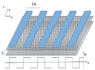
Figure 1: (Color online) Possible realization of the device. An array of ferromagnetic stripes with periodicity $2d_{B}$ placed on top of two monolayer sheets of graphene, produces a periodic magnetic field $B_{z}\simeq\pm B$.

With this magnetic profile, the vector potential in the Dirac Hamiltonian can be fixed by the Landau gauge and chosen periodic in the $x$ direction. The spectrum can then be obtained by a standard transfer matrix approach mckeller : Define ${\cal T}$ (depending on $B$, momentum $k_{y}$ and energy level $\epsilon$) as the transfer matrix that relates the two-component wavefunction on $x$ to its value on $x\pm 2d_{B}$. Showing that $\det{\cal T}=1$ and introducing a new momentum $k_{x}$ due to the periodicity of the superlattice, the eigenvalues of ${\cal T}$ can be written as $e^{\pm 2ik_{x}d_{B}}$, so the condition determining the band structure is

$$\textrm{Tr}\left[{\cal T}(k_{y},\epsilon)\right]=2\cos(2k_{x}d_{B}).$$ (1)

Expanding $\textrm{Tr}\left[{\cal T}(k_{y},\epsilon)\right]$ on $k_{y}$ and $\epsilon$, noting that $\textrm{Tr}\left[{\cal T}(k_{y},0)\right]=2\cosh(2k_{y}d_{B})$, and expanding $\cos(2k_{x}d_{B})$ on $k_{x}$, we then solve Eq. (1) for $\epsilon$. We find that the energy dispersion remains linear and isotropic for small momentum, but with a reduced velocity $\alpha_{d}v_{F}\leq v_{F}$ 6 ; 7 ; 8 ; 9 ,

$$\epsilon_{\pm}({\bf k})=\pm\hbar(\alpha_{d}v_{F})|{\bf k}|\left(1+\delta({\bf k})\right)\ .$$ (2)

In Eq. (2) $\alpha_{d}$ is a function of $d=d_{B}/\ell_{B}$, the dimensionless stripe width, where the magnetic length $\ell_{B}=\sqrt{\hbar c/eB}\simeq 26/\sqrt{B(\mathrm{T})}$ nm. An expansion of Eq. (1) limits the correction term in Eq. (2), $|\delta({\bf k})|\lesssim d_{B}^{2}k_{x}^{2}/6$. The decrease in Fermi velocity in the small and large $d$ limits is 6 ; 9 ,

$$\alpha_{d}\simeq 1-d^{4}/60,\ \ d\ll 1$$ (3)

$$\alpha_{d}\simeq\frac{2d}{\sqrt{\pi}}e^{-d^{2}/4},\ \ d\gg 1\ .$$ (4)

At large densities, $E_{F}$ eventually passes out of the first energy band of the periodic magnetic field into the band gap where the linear spectrum approximation is no longer valid. The energy width $E_{B}$ of the band can be numerically calculated by solving Eq. (1) at the boundaries of the Brillouin zone, $k_{x}=\pm\pi/2d_{B}$, i.e. $\textrm{Tr}[{\cal T}(0,E_{B})]=-2$, with $E_{0}=\hbar v_{F}/\ell_{B}\approx 22\sqrt{B\text{ (Tesla)}}$ meV. We find $E_{0}\alpha_{d}/d\leq E_{B}<E_{0}\pi\alpha_{d}/2d$. The lower limit is valid for large $d$. It corresponds to the spectrum along $k_{x}$ as $\epsilon(k_{x})=\hbar(\alpha_{d}v_{F})\sqrt{[1-\cos(2k_{x}d_{B})]/2}/d_{B}\simeq\hbar(\alpha_{d}v_{F})k_{x}(1-d_{B}^{2}k_{x}^{2}/6)$, the largest deviation from linearity. The upper limit is valid for small $d$. It corresponds to a completely linear spectrum, $\epsilon(k_{x})=\hbar\alpha_{d}v_{F}k_{x}$. Remarkably, along the $k_{y}$ direction the spectrum is found to be almost linear for all $\epsilon\leq E_{B}$ and for all parameters we use. Within linear approximation, we must restrict our results to values of $E_{F}\leq E_{B}$. Even in the least favourable case, when the extreme value $E_{F}=E_{B}$ is reached at $k_{x}=1/d_{B}$ (in the linear approximation), the true spectrum remains close to the linear spectrum, $\epsilon(\frac{1}{d_{B}})=\sqrt{(1-\cos{2})/2}E_{F}\simeq 0.84E_{F}$. This gives an estimate of the maximum error along $k_{x}$. In the superfluid state, $\delta({\bf k})$ must also be small compared with the energy gap $\Delta_{\mathrm{max}}$ since the gap excludes single-particle states lying less than $\Delta_{\mathrm{max}}$ above $E_{F}$, or equivalently, using the limiting value at the Brillouin zone edge, $|\delta({\bf k})|<\pi^{2}/24$,

$$\pi^{3}\alpha_{d}/48d\ll\Delta_{\mathrm{max}}/E_{0}\ .$$ (5)

For $d\gg 1$, Eq. (5) is always satisfied since $\alpha_{d}\sim d\mathrm{e}^{-d^{2}/4}$.

II.2 Enhancement of superfluidity by magnetic field

The effective Hamiltonian for the two monolayer sheets of graphene in the presence of the periodic perpendicular magnetic field is,

$${\cal{H}}\!=\!\sum_{\mathbf{k}\gamma}\xi_{\mathbf{k}}^{\gamma}c^{\gamma\dagger}_{\mathbf{k}}c_{\mathbf{k}}^{\gamma}\!+\!\sum_{\begin{subarray}{c}\mathbf{q}\mathbf{k}\gamma\\ \mathbf{k}^{\prime}\gamma^{\prime}\end{subarray}}V^{eh}_{\mathbf{k}-\mathbf{k}^{\prime}}c^{\gamma\dagger}_{\mathbf{k}+\frac{\mathbf{q}}{2}}c^{\gamma\dagger}_{-\mathbf{k}+\frac{\mathbf{q}}{2}}c^{\gamma^{\prime}}_{\mathbf{k}^{\prime}+\frac{\mathbf{q}}{2}}c^{\gamma^{\prime}}_{-\mathbf{k}^{\prime}+\frac{\mathbf{q}}{2}}\ .$$ (6)

The single-particle energy bands for the modified Dirac cones of the conduction band (electrons) and valence band (holes), $\xi_{\mathbf{k}}^{\gamma}=\gamma\alpha_{d}v_{F}|{\mathbf{k}}|-\mu$, are measured from their respective chemical potentials $\pm\mu$, where $\gamma=1(-1)$ labels the electron (hole) sheet. The $c^{\gamma\dagger}_{\mathbf{k}}$ and $c_{\mathbf{k}}^{\gamma}$ are creation and destruction operators for electrons and holes. Spin indices are implicit. $V^{eh}_{\mathbf{q}}$ is the screened electron-hole interaction.

The mean-field equations at zero temperature for the momentum-dependent superfluid gap functions $\Delta_{\mathbf{k}}^{\gamma}$, and for equal electron and hole densities $n_{+}=n_{-}=n$ are,

$$\Delta_{\mathbf{k}}^{\gamma} = -\frac{1}{\Omega}\sum_{\mathbf{k}^{\prime}\gamma^{\prime}}F^{\gamma\gamma^{\prime}}_{kk^{\prime}}V^{eh}_{\mathbf{k}-\mathbf{k}^{\prime}}\frac{\Delta_{\mathbf{k}^{\prime}}^{\gamma^{\prime}}}{2E_{\mathbf{k}^{\prime}}^{\gamma^{\prime}}}$$ (7)

$$n_{\gamma} = \frac{g_{v}g_{s}}{\Omega}\sum_{\mathbf{k}}\frac{1}{2}\!\left(1-\frac{\xi_{\mathbf{k}}^{\gamma}}{E_{\mathbf{k}}^{\gamma}}\right)\ .$$ (8)

$E_{\mathbf{k}}^{\gamma}=\sqrt{\xi^{\gamma\ 2}_{\mathbf{k}}+\Delta_{\mathbf{k}}^{\gamma\ 2}}$, $g_{s}(g_{v})=2$ are the spin (pseudospin) factors, and $\Omega$ is the sheet area. We retain only the s-wave harmonic in the graphene form factor $F^{\gamma\gamma^{\prime}}_{kk^{\prime}}=1/2$ which comes from the overlap of the single-particle wave-functions in the strong-coupled regime Lozovik2012 .

We self-consistently calculate the screened electron-hole interaction $V^{eh}_{\mathbf{q}}$ within the random phase approximation (RPA) in the zero temperature superfluid state Lozovik2012 ; Perali2013 ; MacDonald2012 . The most favourable conditions for pairing are at small interlayer separations $D$ on the scales of both the effective Bohr radius and the inverse Fermi momentum $k_{F}^{-1}$ in each layer. In this case $qD\ll 1$ and the interaction reduces to,

$$\!V^{eh}_{\mathbf{q}}\!=\!\frac{v_{q}\mathrm{e}^{-qD}}{1+2v_{q}\Pi(q)}\ .$$ (9)

$v_{q}=-2\pi e^{2}/(\kappa q)$ is the unscreened Coulomb interaction. $\Pi(q)=\Pi^{(n)}(q)+\mathrm{e}^{-qD}\Pi^{(a)}(q)\simeq\Pi^{(n)}(q)+\Pi^{(a)}(q)$ is the sum of the normal (intralayer) and anomalous (interlayer) polarizabilities for the superfluid state calculated with the linear energy spectrum. The gap equation [Eq. (7)] is independent of density when expressed in units of $E_{F}$ and $k_{F}$, with the exception of the $\mathrm{e}^{-qD}$ factor in Eq. 9 for $V^{eh}_{\mathbf{q}}$. With increasing density, this factor weakens $V^{eh}_{\mathbf{q}}$.

Figure 2: (Color online) Interaction parameter $r_{s}$ for magnetic field of periodicity $2d$ for dielectric constant $\kappa=3$ (monolayers embedded in a h-BN substrate and $\kappa=2$ (free standing monolayers, separated by h-BN). Superfluidity occurs for $r_{x}\geq r_{s}^{\textrm{onset}}=2.35$ Lozovik2012 .

Rescaling $\tilde{q}=\alpha_{d}q$ gives $\Pi(q,\alpha_{d}v_{F})=\alpha_{d}^{-2}\Pi(\tilde{q},v_{F})$, and, for $\tilde{q}D\ll 1$, $V^{eh}_{\mathbf{q}}(\alpha_{d}v_{F},\kappa)=\alpha_{d}^{2}V^{eh}_{\mathbf{q}}(v_{F},\alpha_{d}\kappa)$. Equations 7 and 8 thus remain the same, but with $(\alpha_{d}\kappa)$ replacing $\kappa$. The interaction parameter $r_{s}=[1/\alpha_{d}][{e^{2}}/({\hbar\kappa v_{F}})]$ increases by a factor $\alpha_{d}^{-1}$.

III Results

Figure 2 shows that by tuning $\alpha_{d}$ with $d$ using a periodic magnetic field, $r_{s}$ can be increased above the value $r_{s}^{\textrm{onset}}$ needed for superfluidity. $\kappa=3$ corresponds to monolayers embedded in a h-BN substrate. $\kappa=2$ corresponds to a free standing system with the two monolayers separated by h-BN. For $d<d_{\textrm{min}}\approx 2\sqrt{\log\kappa}+1$, $r_{s}<r_{s}^{\textrm{onset}}$, and the superfluidity is killed by strong screening. For $\kappa=3(2)$, $d_{\textrm{min}}\approx 3.1(2.7)$.

The renormalization of the band structure is the main effect that drives the superfluidity in the double monolayer system. We find whenever superfluidity occurs, the electron-hole pairs of the superfluid ground state are compact compared with their spacing, making them approximately neutral, and the electrons and holes have opposite wave-vectors. Thus screening effects and effects of the magnetic field on the orbital degrees of freedom should be small compared with the primary effect, the renormalization of the Fermi velocity.

Figure 3 shows the maximum superfluid energy gap $\Delta_{\mathrm{max}}$ at zero temperature for different values of the magnetic field $B$, as a function of sheet density $n$, for two monolayers separated by $D=2$ nm and embedded in a h-BN substrate. The gaps $\Delta_{\mathrm{max}}$ are of the order of several hundred Kelvin. $\Delta_{\mathrm{max}}$ decreases with increasing $n$, due to the $\mathrm{e}^{-qD}$ factor in $V^{eh}_{\mathbf{q}}$ [Eq. 9]. This eventually results in no solution to the gap equation. However, we terminate the curves in Fig. 3 when $E_{F}$ reaches $E_{B}$, and this occurs before such a density is reached. $E_{F}=E_{B}$ thus gives a lower limit on the maximum density for the superfluid phase, $n\simeq 5\times 10^{10}B\mathrm{(T)}/d^{2}$ cm^-2.

For all the gaps shown in Fig. 3, $\Delta_{\mathrm{max}}\gg E_{F}$, leading to a strong suppression of the screening. At higher densities, the very strong screening would kill the superfluidity before the system can enter the BCS regime Perali2013 . However, with increasing density, and well before $\Delta_{\mathrm{max}}$ can drop to $E_{F}$, the Fermi energy reaches the band edge $E_{B}$, where the curve must be truncated.

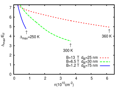
Figure 3: (Color online) Maximum superfluid gap $\Delta_{\mathrm{max}}$ for different values of the magnetic field $B$, as a function of sheet densities $n$. Sheet separation is $D=2$ nm. At arrow points: $\Delta_{\mathrm{max}}$ in Kelvin.

To maximize the density range for superfluidity, the magnetic field $B$ should be made large. In the ferromagnetic stripes shown in Fig. 1, the maximum magnetic field is $B\simeq 1.2$ T, with magnetic length $\ell_{B}\sim 24$ nm. For $\kappa=3$, this corresponds to a minimum stripe width $d_{B}=d_{\textrm{min}}\ell_{B}=74$ nm, readily attainable experimentally. However for $B\lesssim 1.2$ T, the magnetic band width is narrow so that $E_{F}$ reaches $E_{B}$ at low densities (see Fig. 3).

To obtain superfluidity at higher densities, a deformation of the graphene layer can be used to produce much larger pseudo-magnetic fields. Periodic deformations of the graphene layers generate a fictitious vector potential which can produce a periodic pseudo-magnetic field in the layers Low2010 ; Guinea2008 ; Guinea2009a ; guinea_gauge_2009 .

The pseudo magnetic field induced by the strain changes sign for the two valleys. The Dirac cones at the Brillouin zone points $K$ and $K^{\prime}$ will experience an alternating magnetic field in both cases, but with a $\pi$ shift in phase. However, in the absence of intervalley scattering, as considered in this work, a global $\pi$ shift in the zero-flux magnetic field does not affect the renormalization of the Fermi velocity of the two Dirac cones. Therefore, the evaluation procedure for determining the RPA screening and the density of carriers, using two equivalent renormalized Dirac cones, is the same as for the ferromagnetic stripes.

Let us consider a periodic modulation of the graphene layer with height profile [Fig. 4(a)] along the zig-zag direction of the lattice, $h(x,y)=h_{0}\cos\left(2\pi x/\lambda\right)$. $h_{0}$ and $\lambda$ are the modulation amplitude and wavelength. The pseudo-potential $\vec{A}=(A_{x},A_{y})$ at lattice point $\alpha$ is defined as:

$$A_{x}^{\alpha}+iA_{y}^{\alpha}=\frac{1}{ev_{F}}\sum_{\beta\in nn(\alpha)}t_{\alpha\beta}(R_{\alpha\beta})\mathrm{e}^{\left(-i\vec{K}\cdot\vec{R}_{\alpha\beta}\right)}\ .$$ (10)

The $K$ point of the Brillouin zone is at $\vec{K}$, $\vec{R}_{\alpha\beta}$ is the distance between atoms $\alpha$ and $\beta$, and the hopping amplitude $t_{\alpha\beta}$ couples the $p_{z}$ orbitals on neighboring atoms. The corresponding pseudo-magnetic field is $\vec{B}=\vec{\nabla}\times\vec{A}$.

Figure 4(a) shows the profile of the periodic deformation along the zig-zag direction for $\lambda=80$ nm and amplitudes $h_{0}$. Figure 4(b) shows the induced strain, and Fig. 4(c) the induced periodic pseudo-magnetic field. The periodicity of the strain profile and the pseudo-magnetic fields is one-half of $\lambda$, so $\lambda=80$ nm corresponds to a stripe width $d_{B}=20$ nm.

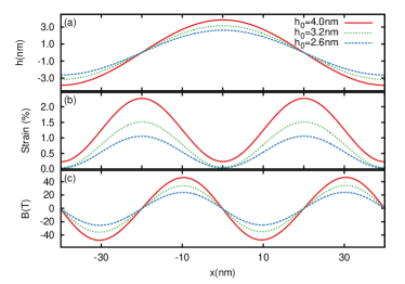
Figure 4: (Color online) (a) Periodic deformation profile $h$ of a graphene sheet. (b) Induced strain in the sheet. (c) Induced pseudo-magnetic field in the sheet.

To explore the modification of the electronic properties induced by an out-of-plane deformation, we have calculated the local density of states (LDOS) using the tight-binding Hamiltonian with a spatially varying hopping amplitude induced by a spatially varying inter-carbon distance. The LDOS is calculated through a Chebyshev expansion of the single particle Green’s function Neek-Amal2012 ; Neek-Amal2013 . For $\lambda=80$ nm, we find that for deformation amplitudes up to $h_{0}<4$ nm, we recover the same phenomenon in the energy dispersion as that for the real magnetic field, an isotropic linear dispersion with the slower Fermi velocity $\alpha_{d}v_{F}$. Figure 4(c) shows that an amplitude $h_{0}\simeq 2.6$ nm generates the large pseudo-magnetic field $B\simeq 20$ T. This leads to a much wider magnetic band width $E_{B}$ than is possible for ferromagnetic stripes, and $E_{F}$ does not reach $E_{B}$ until densities $n>10^{11}$ cm^-2. An experimental realization would be to deposit graphene on a substrate that can be strained through surface acoustic waves (SAWs) Fu2010 , using two inter-digital transducers and a piezo-electric substrate. For wavelengths $\lambda\simeq 80$ nm and typical piezo-electric materials used in SAW devices, the frequency $\sim 50$ GHz.

The Fourier transform of the interaction in Eq. (9) in the presence of graphene corrugations should be evaluated in the periodic curved geometry. However, in the strong coupling regime, the electron-hole pairs have dimensions along the layers comparable to the deformation wave-lengths, so the curved geometry corrections to the interaction will be small.

III.1 Transition temperature

Over the range of parameters we are considering, we find that the electron-hole superfluidity is always in the strong-coupling regime, well inside the crossover regime of the BCS-BEC crossover. The transition temperature calculated within the mean field approach, $T_{mf}$, will be much larger than the actual transition temperature for the onset of phase coherence. A lower bound on the transition temperature in two-dimensions is given by the Kosterlitz-Thouless (KT) temperature,

$$T_{KT}=(\pi/2)\rho_{s}(T_{KT})\ ,$$ (11)

where $\rho_{s}(T)$ is the superfluid stiffness. $\rho_{s}(T=0)=E_{F}/4\pi$ and, when $k_{F}D$ is small, $\rho_{s}(T)$ falls off slowly with $T$ for $T\ll\Delta_{\mathrm{max}}$. Hence taking $\rho_{s}(T)\simeq\rho_{s}(0)$, we obtain $T_{KT}=E_{F}/8$ for $E_{F}/8\ll\Delta_{\mathrm{max}}$.

Since in general $T_{KT}\ll T_{mf}$, the mean field superfluid gap will be insensitive to $T$ for $T\leq T_{KT}$. By a similar argument, the RPA screening polarization bubbles are only weakly affected by finite $T\leq T_{KT}$. Thus, in the superfluid calculations we can take $T=0$.

For superfluidity to occur, we recall that the array spacing $d\gtrsim 3$ (Fig. 2). For these values of $d$, the linearized Eq. (2) is valid whenever $E_{F}<E_{B}$ is satisfied. This inequality establishes an upper bound on the maximum transition temperature, $T_{KT}\leq T_{KT}^{\textrm{max}}\simeq 35\sqrt{B\mathrm{(Tesla)}}\exp{(-d^{2}/4)}$ K, the equality occurring for $E_{F}=E_{B}$. Figure 5 shows this maximum $T_{KT}^{\textrm{max}}$ as a function of both $B$ and $d$.

Figure 5: (Color online) (a) $T_{KT}^{\textrm{max}}$ as a function of $B$. Array spacings $d=3.1$ and $2.7$ give maximum transition temperature for embedded and free-standing system, respectively. (b) $T_{KT}^{\textrm{max}}$ as a function of $d$.

IV Conclusions

We have proposed an electron-hole double monolayer graphene system, in which a quantum phase transition to a superfluid is induced by a periodic magnetic field. Electron-hole pairing in conventional double monolayers is known to be severely weakened by screening within the layers which kills the superfluidity. If the pairing can be made strong, then a large superfluid gap is known to open up, destroying the low-energy single-particle excitations that cause the screening. We show how a periodic magnetic field applied perpendicular to the monolayers could be used for this purpose: The field preserves the isotropic Dirac cones of the original monolayers but reduces the Fermi velocity in a tunable way, shifting the system parameters into the strongly coupled pairing regime where screening is sufficiently weakened for finite-temperature electron-hole superfluidity to occur.

- (1) Hongki Min, Rafi Bistritzer, Jung-Jung Su, and A. H. MacDonald, Phys. Rev. B 78, 121401(R) (2008).
- (2) Yu. E. Lozovik, S. L. Ogarkov, and A. A. Sokolik, Phys. Rev. B 86, 045429 (2012).
- (3) I. Block, J. Dalibard, and W. Zwerger, Rev. Mod. Phys. 80, 885 (2008); A. Perali, F. Palestini, P. Pieri, G. C. Strinati, J. T. Stewart, J. P. Gaebler, T. E. Drake, and D. S. Jin, Phys. Rev. Lett. 106, 060402 (2011).
- (4) A. Perali, D. Neilson, and A. R. Hamilton, Phys. Rev. Lett. 110, 146803 (2013).
- (5) K. V. Germash and D. V. Fil, Phys. Rev. B 91, 115442 (2015).
- (6) R. V. Gorbachev, A. K. Geim, M. I. Katsnelson, K. S. Novoselov, T. Tudorovskiy, I. V. Grigorieva, A. H. MacDonald, K. Watanabe, T. Taniguchi, L. A. Ponomarenko, Nat. Phys. 8, 896 (2012).
- (7) D. S. L. Abergel, M. Rodriguez-Vega, Enrico Rossi, and S. Das Sarma, Phys. Rev. B 88, 235402 (2013).
- (8) D. Neilson, A. Perali, and A. R. Hamilton, Phys. Rev. B 89, 060502(R) (2014).
- (9) M. Zarenia, A. Perali, D. Neilson, and F. M. Peeters, Sci. Rep. 4, 7319 (2014).
- (10) A.F. Croxall, K. Das Gupta, C.A. Nicoll, M. Thangaraj, H. E. Beere, I. Farrer, D. A. Ritchie, and M. Pepper, Phys. Rev. Lett. 101, 246801 (2008).
- (11) J. A. Seamons, C. P. Morath, J. L. Reno, and M. P. Lilly, Phys. Rev. Lett. 102, 026804 (2009).
- (12) A. Gamucci, D. Spirito, M. Carrega, B. Karmakar, A. Lombardo, M. Bruna, L. N. Pfeiffer, K. W. West, A. C. Ferrari, M. Polini, and V. Pellegrini, Nat. Commun. 5, 5824 (2014).
- (13) L. Dell’Anna and A. De Martino, Phys. Rev. B 79, 045420 (2009); ibid. 80, 089901(E) (2009).
- (14) I. Snyman, Phys. Rev. B 80, 054303 (2009).
- (15) L. Z. Tan, C.-H. Park, and S. G. Louie, Phys. Rev. B 81, 195426 (2010).
- (16) L. Dell’Anna and A. De Martino, Phys. Rev. B 83, 155449 (2011).
- (17) M. Barbier, P. Vasilopoulos, and F. M. Peeters, Phys. Rev. B 81, 075438 (2010).
- (18) M. Cerchez, S. Hugger, T. Heinzel, and N. Schulz, Phys. Rev. B 75, 035341 (2007).
- (19) B. H. J. McKellar and G. J. Stephenson, Jr., Phys. Rev. C 35, 2262 (1987).
- (20) I. Sodemann, D.A. Pesin, and A.H. MacDonald, Phys. Rev. B 85, 195136 (2012).
- (21) Tony Low and F. Guinea, Nano Lett. 10, 3551 (2010).
- (22) F. Guinea, M. I. Katsnelson, and M. A. H. Vozmediano, Phys. Rev. B 77, 075422(2008).
- (23) F. Guinea, M. I. Katsnelson, and A. K. Geim, Nat. Phys. 6, 30 (2009).
- (24) F. Guinea, B. Horovitz, and P. Le Doussal, Solid State Commun. 149, 1140 (2009).
- (25) M. Neek-Amal, L. Covaci, and F. M. Peeters, Phys. Rev. B 86, 041405 (2012).
- (26) M. Neek-Amal, L. Covaci, K. Shakouri, and F. M. Peeters, Phys. Rev. B 88, 115428 (2013).
- (27) Y. Fu, J. Luo, X. Du, A. Flewitt, Y. Li, G. Markx, A. Walton, and W. Milne, Sens. Actuators, B 143, 606 (2010).