NuSTAR and Swift observations of the black hole candidate XTE J1908+094 during its 2013 outburst

Abstract

The black hole candidate XTE J1908+094 went into outburst for the first time since 2003 in October 2013. We report on an observation with the Nuclear Spectroscopic Telescope Array (NuSTAR) and monitoring observations with Swift during the outburst. NuSTAR caught the source in the soft state: the spectra show a broad relativistic iron line, and the light curves reveal a $\sim$40 ks flare with the count rate peaking about 40% above the non-flare level and with significant spectral variation. A model combining a multi-temperature thermal component, a power-law, and a reflection component with an iron line provides a good description of the NuSTAR spectrum. Although relativistic broadening of the iron line is observed, it is not possible to constrain the black hole spin with these data. The variability of the power-law component, which can also be modeled as a Comptonization component, is responsible for the flux and spectral change during the flare, suggesting that changes in the corona (or possibly continued jet activity) are the likely cause of the flare.

1. Introduction

XTE J1908+094 is an X-ray transient serendipitously discovered with the Rossi X-ray Timing Explorer (RXTE) Proportional Counter Array (PCA) when it went into outburst in 2002 February (Woods et al., 2002). The source flux in the 2–10 keV band rose by a factor of $\sim$3 in one month (Woods et al., 2002) and reached about 100 mCrab on 2002 April 6 (Göǧüş et al., 2004). The power density spectrum showed a broad quasi-periodic oscillation (QPO) at 1 Hz without any coherent pulsation between 0.001 and 1024 Hz (Woods et al., 2002). In the X-ray energy spectrum, an iron emission line and a hard tail up to 250 keV were detected (Woods et al., 2002; Feroci et al., 2002). The hard X-ray spectrum did not agree with an extrapolation of the absorbed power-law model in the 2–30 keV band reported by Woods et al. (2002), and showed a high-energy cut-off at $\sim$ 100 keV (Feroci et al., 2002). Given the timing and spectral characteristics, XTE J1908+094 is suggested to be a black hole candidate (Woods et al., 2002; Feroci et al., 2002; in’t Zand et al., 2002; Göǧüş et al., 2004).

The broad band X-ray spectrum of XTE J1908+094 is well fitted with two continuum components, a multi-temperature disk blackbody with $kT$ $\sim$ 0.8 keV and a Compton plasma with a temperature near 40 keV, and an emission line centered on the location of the Fe K$\alpha$ line (in’t Zand et al., 2002). The emission feature is very broad with FWHM$=3.2\pm 0.5$ keV (line width $\sigma=1.4\pm 0.2$ keV), which may be due to Compton scattering in a corona or the relativistic effects from gravitational redshift and Doppler broadening of orbital motion (in’t Zand et al., 2002). In the latter case, the broadening of the Fe emission line would be expected to be asymmetric, and could be used to measure the black hole (BH) spin (Reynolds & Nowak, 2003; Miller, 2007). Based on this method, Miller et al. (2009) measured the dimensionless spin of XTE J1908+094 to be $a=0.75\pm 0.09$.

The radio counterpart of XTE J1908+094 was discovered with the Very Large Array (VLA) at R.A.=$19^{\rm h}08^{\rm m}53.\!^{\rm s}077$, Decl.=+$09^{\circ}23^{\prime}04.\!^{\prime\prime}90$ (J2000.0) (Rupen et al., 2002), which is consistent with the Chandra position, R.A.=$19^{\rm h}08^{\rm m}53.\!^{\rm s}07$, Decl.=+$09^{\circ}23^{\prime}05.\!^{\prime\prime}0$ (Jonker et al., 2004). Chaty et al. (2002) identified a likely near-infrared (NIR) counterpart for the source, but the possible counterpart was resolved into two sources separated by $\sim$ 0.8 arcsec in subsequent observations (Chaty et al., 2006). Both potential counterparts are consistent with XTE J1908+094 being a low mass X-ray binary (LMXB). One of the NIR sources would indicate an intermediate/late type (A-K) main-sequence companion star, while the other would indicate a late-type main-sequence companion star with spectral type later than K (Chaty et al., 2006). Recently, Swift/UVOT observed the X-ray source; however, no counterpart was found in the $V$ band with the 3$\sigma$ limiting magnitude to be $V>20.3$ (Krimm et al., 2013b).

The distance to XTE J1908+094 is not well established. Based on its X-ray flux, the source is suggested to be at a distance greater than 3 kpc (in’t Zand et al., 2002). From the optical measurements, the possible distance range is 3–10 kpc (Chaty et al., 2006). An estimate using the X-ray and radio fluxes puts the source at a distance of $\sim$ 2–10 kpc (Miller-Jones et al., 2013).

Previously, XTE J1908+094 went through two outbursts in 2002 and early 2003 with very similar spectral evolution (Göǧüş et al., 2004). On 2013 October 26, another outburst of XTE J1908+094 was detected by the Swift Burst Alert Telescope (BAT), with the 15–50 keV flux reaching $\sim$ 60 mCrab two days later (Krimm et al., 2013a). Subsequently, a number of telescopes, including NuSTAR, Swift (Krimm et al., 2013a, b), the VLA (Miller-Jones et al., 2013), the Arcminute Microkelvin Imager (AMI) Large Array (Rushton et al., 2013a), the Monitor of All-sky X-ray Image (MAXI, Negoro et al., 2013) and the Australia Telescope Compact Array (ATCA, Coriat et al., 2013) carried out observations of the source. In this paper, we report on the NuSTAR and Swift observations of the 2013 outburst in detail (Section 2) and investigate its spectral evolution and properties (Section 3). We present a discussion of the results in Section 4 and conclusions in Section 5.

2. Observations

XTE J1908+094 was monitored with many short observations by the Swift/X-ray Telescope (XRT) (Burrows et al., 2005) from 2013 October 26 to 2013 December 3, and NuSTAR (Harrison et al., 2013) carried out an observation with an effective exposure time of $\sim$ 45 ks on 2013 November 8. In order to study the outburst properties of the source, we used the NuSTAR observation and all of the Swift/XRT observations that were long enough to achieve sufficient statistical quality (see Table 1 for the observation list).

Table 1NuSTAR and Swift Observations

ObsID	Observed date	Exposure (s)
NuSTAR
80001014002	2013-11-08	45061/45404a
Swift XRT
00033014001	2013-10-29	972
00033014002	2013-11-01	1224
00033014003	2013-11-03	1032
00033014004	2013-11-08	1044
00033014005	2013-11-09	1007
00033014006	2013-11-10	503
00033014007	2013-11-11	880
00033014008	2013-11-12	975
00033014009	2013-11-13	1343
00033014010	2013-11-14	792
00033014011	2013-11-15	1085
00033014012	2013-11-16	1150
00033014014	2013-11-18	979
00033014015	2013-11-19	1008
00033014016	2013-11-20	978
00033014017	2013-11-23	958
00033014018	2013-11-28	824
00033014019	2013-12-03	976

Note. — ^a The exposure times of NuSTAR FPMA and FPMB, respectively. The Swift XRT data are taken in windowed mode.

2.1. NuSTAR

The NuSTAR data (ObsID 80001014002) were processed using version 1.3.1 of the NuSTARDAS pipeline with NuSTAR CALDB version 20131223. The spectra and light curves were extracted from a region centered at the position of XTE J1908+094 with a radius of 120$\arcsec$. The source region was contaminated by stray light from the nearby bright source GRS 1915+105. Thus, the background region was chosen carefully. We used a circular background region with a radius of 80$\arcsec$ from the part of the field of view that was illuminated by the GRS 1915+105 stray light and as far away from XTE J1908+094 as possible. The background count rate is less than 6% of the source count rate, which means that, even considering the stray light, the source still strongly dominates the spectra and light curves. The spectra of the two $NuSTAR$ focal plane modules A and B (FPMA and FPMB), were rebinned to have at least 50 counts per bin. The light curves were binned to a time resolution of 100 s.

2.2. Swift

We reduced the Swift/XRT data from 2013 October 29 to 2013 December 3 (see Table 1). All data were taken in windowed timing mode. Using XSELECT with XRT CALDB version 20140709, the spectra were extracted from a circular region with a radius of 20 pixels ($\sim 47\arcsec$). The background extraction region is a box 20 pixels long, centered 100 pixels from the middle of the source extraction region. Ancillary response files were created using the ftool xrtmkarf. At lower energies, the windowed timing mode shows a bump between 0.4-1 keV and a turn up at the lowest energies. In order to reduce the low-energy spectral residuals, the grade 0 data and the position-dependent response matrices from the latest XRT calibration files were used. Finally, the extracted spectra were rebinned to contain a minimum of 25 counts per bin.

Figure 1.— From top to bottom, the 15-50 keV Swift/BAT count rate, the 0.3-10 keV Swift/XRT count rate and the hardness ratio between the Swift/XRT hard band (2.5-10 keV) and soft band (0.3-2.5 keV). Two vertical dashed lines indicate the time boundaries of the NuSTAR observation.

Figure 2.— The evolution of Swift/XRT spectral parameters. (a) photon index $\Gamma$ and reduced $\chi^{2}$ when fitting with a single absorbed power-law model; (b) photon index $\Gamma$, inner disk temperature $T_{\rm in}$, normalization of the diskbb model and reduced $\chi^{2}$ when fitting with a two-component model consisting of power-law and disk components. The arrows indicate the upper limit of $\Gamma$ where the lower error bars of $\Gamma$ could not be well constrained. Two vertical dotted lines show the time interval of the NuSTAR observation.

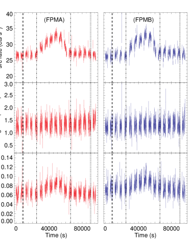
Figure 3.— The NuSTAR observation of XTE J1908+094. Top: the 3–79 keV light curves of XTE J1908+094 observed by FPMA and FPMB, respectively. Middle: the background light curves in the 3–79 keV band. Bottom: the hardness ratio defined as the ratio of the count rates in the 10–79 keV to 3–10 keV bands. The two vertical dash-dotted lines exhibit the duration of the flare, the two vertical dashed lines show the time interval of Swift observation ObsID 00033014004, and the two vertical dotted lines indicate Swift observation ObsID 00033014005.

3. Results

3.1. Swift Monitoring

The Swift monitoring observations reveal a clear evolution starting from 2013 October 25 (MJD 56590) (see Figure 1). The Swift/BAT count rate in the 15–50 keV band increased rapidly from $0.0022\pm 0.0008$ $\rm cts~{}cm^{-2}~{}s^{-1}$ on MJD 56590 to $0.026\pm 0.002$ $\rm cts~{}cm^{-2}~{}s^{-1}$ on MJD 56595 and then decreased sharply to $\sim 0.0015$ $\rm cts~{}cm^{-2}~{}s^{-1}$ and stayed close to that level after MJD 56604. In Swift/XRT’s 0.3–10 keV band, the source brightened from $9.2\pm 0.1$ $\rm cts~{}s^{-1}$ on MJD 56595, reaching its peak count rate of $36.2\pm 0.2$ $\rm cts~{}s^{-1}$ on MJD 56607 and then dimmed. The hardness, defined as the ratio of the count rates in the 2.5–10 keV to 0.3–2.5 keV bands, started to decrease from $2.15\pm 0.05$ on MJD 56595 to $1.030\pm 0.011$ on MJD 56605, and then stayed at a value of $\sim 1$. All of these measurements suggest that the source entered a state transition around MJD 56595 and was in the soft state 10 days later. The long exposure obtained with NuSTAR between MJD 56605 and MJD 56606 occurred after the source reached the soft state.

First, we fitted the 0.5–10 keV Swift/XRT spectra using a single absorbed power-law model. The Swift data below 0.5 keV were ignored during the spectral fits in order to exclude the low-energy spectral residuals in windowed timing mode. The values of the photon index, $\rm\Gamma$, and the reduced $\chi^{2}$ are plotted in Figure 2a. The value of $\Gamma$ increased steeply from 1.6 on MJD 56595 to 4.4 on MJD 56605, and remained at $\sim 4.5$ until MJD 56629, consistent with the source going through the hard to soft state transition. After the source begins the state transition, the accretion disk is significant for most of the observation. For these observations, a single power-law does not provide a good fit to the spectra, and the addition of a disk-blackbody component provides a significant improvement to the fit. The inner disk temperature $T_{\rm in}$, the normalization of the diskbb model, the photon index $\Gamma$, and the reduced $\chi^{2}$ are shown in Figure 2b. The absorbed disk blackbody plus power-law model could successfully fit all spectra, with $T_{\rm in}$ increasing from 0.3 before the state transition and stabilizing at about 0.7–0.8 keV in soft state.

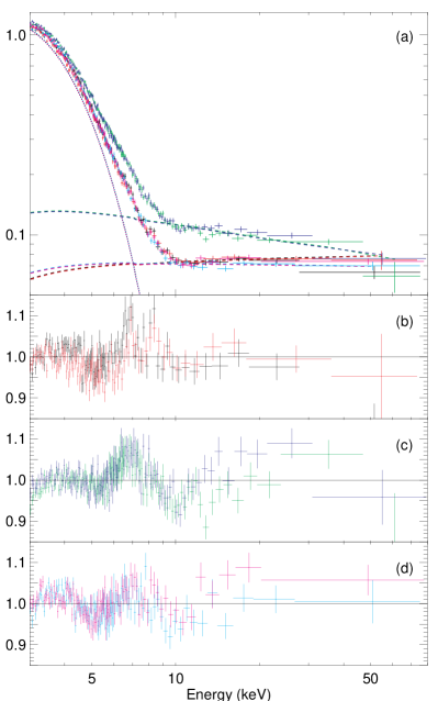
Figure 4.— The NuSTAR spectra, model and residuals. (a) the unfolded NuSTAR spectra and model in $E^{2}\ast f(E)$ representation. The model includes a fixed disk blackbody component and a free power-law model before, during and after the flare. Black and red crosses are NuSTAR FPMA and FPMB spectra before the flare, respectively; green and blue crosses indicate the spectra during the flare; cyan and magenta crosses indicate the spectra after the flare. The top dotted line exhibits the disk blackbody component, and the three lower dashed lines show the power-law components during the different stages. The power-law component is stronger during the flare, while the power-law components before and after the flare show fluxes that are lower and similar to each other. Also, the power-law index of the flare is softer than those of the non-flare spectra. (b) – (d) Data/model ratio before, during and after the flare, respectively.

3.2. NuSTAR Spectroscopy

The NuSTAR light curves of FPMA and FPMB (see the top panels of Figure 3) with background subtraction show a flare of $\sim 40$ ks duration with the peak rate being $\sim$40% above the non-flare rate. The background light curves are also shown in Figure 3 in order to evaluate if the variability might be from the nearby source GRS 1915+105 rather than XTE J1908+094. The background light curves are stable at an average value of 1.3 $\rm cts~{}s^{-1}$, less than 6% of the net source count rate. Thus, although the high background caused by GRS 1915+105 affects the statistical quality of the XTE J1908+094 spectrum, Figure 3 demonstrates that the flare in the light curves comes from XTE J1908+094. To study whether the flare has a different spectrum from the non-flare emission, we first checked the ratios of the 10–79 keV count rates to the 3-10 keV count rates. During the flare, this hardness ratio increased (bottom panels of Figure 3), indicating that there is spectral variation.

To investigate further, we extracted the 3–79 keV spectra prior to the flare, during the flare and after the flare and fitted them together using a simple model combining an energy-independent multiplicative factor (constant), an absorption model (tbabs), adopting abundances from Wilms et al. (2000), a power-law model (pegpwrlw) and a multi-temperature disk-blackbody model (diskbb), i.e, constant $\ast$ tbabs $\ast$ (pegpwrlw + diskbb). Untying the model parameters individually or in combination, we found that only changing the power-law model could explain the variability, with a reduced $\rm\chi^{2}=1.25$ for 2697 degrees of freedom (dof). As shown in the top panel of Figure 4, the power-law component changes significantly between the flare and non-flare spectra: before the flare, $\Gamma=1.96$, during the flare, $\Gamma=2.23$, and after the flare, $\Gamma=2.03$. Here, we quote the best fit parameters without error bars because this simple model does not provide an acceptable fit to the data. Moreover, as shown in Figure 4b, c and d, all spectra exhibit similar residuals when the power-law parameters are allowed to vary prior to the flare, during the flare and after the flare. Very poor fits are obtained if the power-law component is required to be the same for all three spectra. All of this suggests that the corona, rather than the mass accretion rate and the accretion disk, went through great changes during the NuSTAR observation.

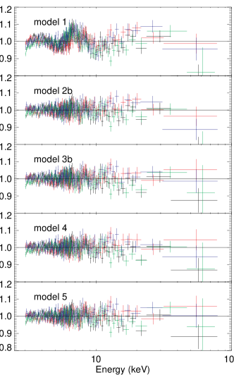
Figure 5.— The residuals for the best fit in different models. Black and red symbols are NuSTAR FPMA and FPMB spectra in the non-flare state; green and blue symbols are the spectra of the flare.

Table 2Spectral fitting of XTE J1908+094: part I

Model	$C$	$N_{\rm H}$	$\Gamma_{1}$	$N_{\rm PL1}$	$E_{\rm cent1}$	$\sigma_{1}$	$N_{\rm gauss1}$	$kT$	$N_{\rm disk}$	$\chi^{2}/{\rm dof}$
			$\Gamma_{2}$	$N_{\rm PL2}$	$E_{\rm cent2}$	$\sigma_{2}$	$N_{\rm gauss2}$
1	$0.993$	$1.6$	$2.00$	$385$	$\cdots$	$\cdots$	$\cdots$	$0.783$	$650$	2709.8/2099
			$2.23$	$554$	$\cdots$	$\cdots$	$\cdots$
2a	$0.993\pm 0.003$	$2.5^{\star}$	$1.95\pm 0.03$	$387\pm 4$	$6.82^{+0.14}_{-0.16}$	$0.98^{+0.15}_{-0.14}$	$0.74^{+0.17}_{-0.14}$	$0.755\pm 0.003$	$873^{+20}_{-19}$	2321.7/2094
			$2.15\pm 0.03$	$545^{+5}_{-6}$	$6.1^{+0.3}_{-0.4}$	$1.3^{+0.3}_{-0.2}$	$2.2^{+1.0}_{-0.6}$
2b	$0.993\pm 0.003$	$5.8^{+0.8}_{-0.6}$	$1.99\pm 0.03$	$391\pm 4$	$5.3^{+0.6}_{-1.0}$	$1.6^{+0.3}_{-0.2}$	$5^{+7}_{-2}$	$0.671^{+0.018}_{-0.026}$	$2300^{+800}_{-400}$	2207.8/2093
			$2.16\pm 0.03$	$551\pm 6$	$4.9^{+0.5}_{-0.9}$	$1.8^{+0.3}_{-0.2}$	$10^{+8}_{-4}$

Note. —

Model 1: constant $\ast$ tbabs $\ast$ (pegpwrlw + diskbb).

Model 2: constant $\ast$ tbabs $\ast$ (pegpwrlw + gaussian + diskbb); 2a: fixed $N_{\rm H}$ at $2.5\times 10^{22}~{}\rm cm^{-2}$; 2b: $N_{\rm H}$ was set as a free parameter.

Model 1 is not an acceptable fit to the spectrum so we just quote the best fit parameters without error bars.

^⋆: fixed value;

$C$ is the NuSTAR FPMB normalization factor relative to FPMA;

$N_{\rm H}$ is the X-ray absorption column density in units of $10^{22}~{}\rm cm^{-2}$;

$\Gamma_{1}$ and $\Gamma_{2}$ are the power-law photon indices of the non-flare and flare spectra;

$N_{\rm PL1}$ and $N_{\rm PL2}$ are the power-law component flux normalizations over the 3–79 keV energy band in units of $\rm 10^{-12}$ erg cm^-2 s^-1;

$E_{\rm cent1}$ and $E_{\rm cent2}$ are the Gaussian emission line energies in keV;

$\sigma_{1}$ and $\sigma_{2}$ are the line widths in keV;

$N_{\rm gauss1}$ and $N_{\rm gauss2}$ are the Gaussian component normalizations in units of $\rm 10^{-3}~{}photons~{}cm^{-2}~{}s^{-1}$;

$kT$ is the accretion disk temperature of the diskbb model in units of keV;

$N_{\rm diskbb}$ is the normalization of the diskbb model;

All errors and limits are at 90% confidence level.

Given the strong spectral variability during the flare and the similar spectral properties before the flare and after the flare, the NuSTAR data in the 3–79 keV band was divided into two parts: the flare spectra and non-flare spectra. The two Swift/XRT observations, ObsID 00033014004 and 00033014005, from prior to the flare and after the flare, respectively (see Figure 3), were combined with the non-flare spectra. Then, we used the model constant $\ast$ tbabs $\ast$ (pegpwrlw + diskbb) (model 1) to fit the flare spectra plus combined non-flare spectra, and freed the power-law component in these two data sets. We find that Swift/XRT and NuSTAR have residuals that are not consistent with each other in the soft X-ray region where they overlap. The residuals are also not the same for the two Swift observations. Note that the exposure times of the Swift observations are about 1 ks (see Table 1), much shorter than that of NuSTAR, allowing for the possibility that Swift might catch short-term spectral variations in its short snapshots. For NuSTAR, the largest residuals are in the iron K$\alpha$ emission line region (Figure 4b, c and d) rather than in the soft X-ray band observed by Swift. Therefore, in the following, we fit the NuSTAR spectra alone.

Table 3Spectral fitting of XTE J1908+094: part II

Para.	Model 3a	Model 3b	Model 4	Model 5
$C$	$0.993\pm 0.003$	$0.993\pm 0.003$	$0.993\pm 0.003$	$0.993\pm 0.003$
$N_{\rm H}$	$4.1\pm 0.3$	$4.4\pm 0.3$	$5.1^{+0.4}_{-0.3}$	$5.3\pm 0.4$
$\Gamma_{1}$	$1.84^{+0.04}_{-0.06}$	$2.01^{+0.04}_{-0.05}$	$2.02\pm 0.04$	$2.02^{+0.05}_{-0.07}$
$\Gamma_{2}$	$2.02^{+0.04}_{-0.05}$	$2.15^{+0.04}_{-0.05}$	$2.16^{+0.05}_{-0.04}$	$2.20\pm 0.04$
$E_{\rm fold1}$	$100^{\star}$	$500^{\star}$	$500^{\star}$	$500^{\star}$
$E_{\rm fold2}$	$100^{\star}$	$500^{\star}$	$500^{\star}$	$500^{\star}$
$N_{\rm PL1}$	$0.027^{+0.012}_{-0.018}$	$0.033^{+0.017}_{-0.024}$	$0.036^{+0.019}_{-0.027}$	$\cdots$
$N_{\rm PL2}$	$0.05^{+0.02}_{-0.03}$	$0.03^{+0.05}_{-0.03}$	$0.06\pm 0.06$	$\cdots$
$f_{\rm scat1}$	$\cdots$	$\cdots$	$\cdots$	$0.010\pm 0.010$
$f_{\rm scat2}$	$\cdots$	$\cdots$	$\cdots$	$0.016^{+0.010}_{-0.012}$
$kT$	$0.719\pm 0.007$	$0.711\pm 0.007$	$0.689^{+0.008}_{-0.012}$	$\cdots$
$N_{\rm diskbb}$	$1310^{+110}_{-100}$	$1420^{+120}_{-110}$	$1810^{+240}_{-160}$	$\cdots$
$M_{\rm BH}$	$\cdots$	$\cdots$	$\cdots$	$2.8^{+15.7}_{-0.2}$
$\dot{M}$	$\cdots$	$\cdots$	$\cdots$	$1.3^{+6.6}_{-0.7}$
$D_{\rm BH}$	$\cdots$	$\cdots$	$\cdots$	$10^{\star}$
$N_{\rm kerrbb}$	$\cdots$	$\cdots$	$\cdots$	$1.7^{+4.9}_{-0.8}$
$\rm\xi_{1}$	$5300^{+1300}_{-1600}$	$4200^{+1300}_{-1000}$	$9000^{+7000}_{-3000}$	$5700^{+1200}_{-1900}$
$\rm\xi_{2}$	$10400\pm 1700$	$10000\pm 2000$	$19500^{+500}_{-6800}$	$11900^{+2300}_{-1500}$
$N_{\rm ref1}$	$1.33^{+0.16}_{-0.15}$	$2.4^{+0.8}_{-0.7}$	$1.2^{+0.5}_{-0.6}$	$2.4^{+0.4}_{-0.3}$
$N_{\rm ref2}$	$1.46\pm 0.14$	$2.4^{+0.9}_{-0.7}$	$1.2\pm 0.5$	$2.2\pm 0.3$
Fe/solar	$1.5^{\star}$	$0.9^{+0.5}_{-0.3}$	$4.0^{+8.4}_{-1.5}$	$1.5^{\star}$
$a$	$\cdots$	$\cdots$	$-0.998^{+1.9}_{-0}$	$-0.96^{+1.63}_{-0.04}$
$i$	$\cdots$	$\cdots$	$27^{+7}_{-4}$	$33^{+3}_{-4}$
$\chi^{2}/{\rm dof}$	2256.9/2095	2227.7/2094	2209.5/2092	2208.5/2092

Note. —

Model 3: constant $\ast$ tbabs $\ast$ (reflionx_hc + cutoffpl + diskbb); 3a: fix $\rm E_{\rm fold}=100$ keV and $\rm{\tt Fe/solar}=1.5$; 3b: fix $\rm E_{\rm fold}=500$ keV and thaw Fe/solar.

Model 4: constant $\ast$ tbabs $\ast$ (relconv $\ast$ reflionx_hc + cutoffpl + diskbb).

Model 5: constant $\ast$ tbabs $\ast$ (relconv $\ast$ reflionx_hc + simpl $\ast$ kerrbb).

$E_{\rm fold1}$ and $E_{\rm fold2}$ are the folding energy of exponential rolloff for the non-flare and flare spectra in units of keV;

$N_{\rm PL1}$ and $N_{\rm PL2}$ are the cutoff power-law normalizations at 1 keV in photons keV^-1cm^-2s^-1;

$f_{\rm scat1}$ and $f_{\rm scat2}$ are the scattered fractions of the simpl model ;

$M_{\rm BH}$ is the black hole mass in units of the solar mass;

$\dot{M}$ is the disk mass accretion rate in units of $10^{18}$ g sec^-1;

$D_{\rm BH}$ is the distance of the black hole in units of kpc;

$N_{\rm kerr}$ is the normalization of the kerrbb model;

$\rm\xi_{1}$ and $\rm\xi_{2}$ are the ionization parameters of the reflionx_hc model in units of $\rm erg~{}cm~{}s^{-1}$;

$N_{\rm ref1}$ and $N_{\rm ref2}$ are the normalizations of reflected spectrum (reflionx_hc) in units of $10^{-7}$;

Fe/solar is the abundance of iron relative to solar value;

$a$ is the dimensionless black hole spin;

$i$ is the inclination angle of the accretion disk in units of degree;

other parameters are the same as in Table 2. All errors and limits are at 90% confidence level.

As shown in Figure 4 and 5, a strong reflection component is apparent in the residuals of this fit (model 1), leading to a large reduced $\rm\chi^{2}=2709.8$ for 2099 dof (see Table 2). Similar to some other Galactic X-ray binaries, the reflection component is composed of an iron K$\alpha$ emission line and a broad reflection excess (Lightman & White, 1988; Miller, 2007; Tomsick et al., 2014). The emission line feature was also detected in the 2002 outburst (in’t Zand et al., 2002; Göǧüş et al., 2004). Following in’t Zand et al. (2002) and Göǧüş et al. (2004), we used the Gaussian emission line model gaussian to fit this feature and performed fits with the neutral hydrogen column density, $N_{\rm H}$, fixed to $2.5\times 10^{22}~{}\rm cm^{-2}$ (model 2a). We also tested fits where $N_{\rm H}$ was a free parameter (model 2b). Adding a Gaussian significantly improves the spectral fits with $\Delta{\chi^{2}}\gtrsim 400$ (see Table 2 and Figure 5). The unabsorbed disk flux fractions, i.e., the relative disk flux contribution to the total, unabsorbed flux in the 2–20 keV range, are larger than 80% for both the flare and non-flare spectra, which meet the soft state criterion of McClintock & Remillard (2006) and also confirm that the NuSTAR observation was taken in the soft state. The measurement of Gaussian line centroid, $E_{\rm cent}$, is dependent on $N_{\rm H}$. Freezing $N_{\rm H}$ at $2.5\times 10^{22}~{}\rm cm^{-2}$, $E_{\rm cent}$ is in the iron line region (6.4 – 7.1 keV); leaving $N_{\rm H}$ as a free parameter, $E_{\rm cent}$ is well below this energy region. Given this, we then tested fits with $N_{\rm H}$ fixed at $4.3\times 10^{22}~{}\rm cm^{-2}$, the average $N_{\rm H}$ when fitting the Swift spectra in soft state with a two component model consisting of power-law and disk components (Section 3.1). We obtained $E_{\rm cent1}=6.2^{+0.2}_{-0.3}$ keV and $E_{\rm cent2}=5.9\pm 0.3$ keV, and the line widths $\sigma_{1}=1.29^{+0.16}_{-0.14}$ keV and $\sigma_{2}=1.51^{+0.19}_{-0.18}$ keV, respectively, for the non-flare and flare spectra, with $\chi^{2}/{\rm dof}=2224.1/2094$.

Instead of the Gaussian emission line model, we then used the more physical model reflionx_hc to fit the reflection component, and replaced the simple power-law model by a power-law with an exponential cutoff cutoffpl (model 3). The reflionx_hc model is an update of the model reflionx (Ross et al., 1999; Ross & Fabian, 2005), which calculates the reflected spectrum from an optically thick atmosphere ionized by illuminating X-rays with a cutoff power-law spectrum. The power-law photon index of reflionx_hc is linked to that of cutoffpl. Compared with reflionx, the folding energy HighECut in reflionx_hc is a free parameter also linked to that of cutoffpl. In addition, the ionization parameter, $\rm\xi$, and the abundance of iron, Fe/solar, extend over larger ranges in reflionx_hc.

When left as a free parameter, the best fit value for the exponential folding energy, HighECut, is 500 keV, which is the upper limit of the parameter range. As this parameter is not well-constrained, we performed fits with HighECut fixed at 100 keV and 500 keV, respectively. Moreover, we also performed fits with Fe/solar fixed at the initial value of 1.5 and as a free parameter. Good fits with reduced $\rm\chi^{2}$ less than 1.08 were obtained if a reflection component was added. Changing HighECut from 100 keV to 500 keV, or unfreezing Fe/solar, other model parameters change only slightly, as seen for model 3a ($\rm\tt{HighECut}=100keV$, $\rm{\tt Fe/solar}=1.5$) and model 3b ($\rm\tt{HighECut}=500keV$, free Fe/solar) in Table 3. Similar to the power-law photon index, the ionization parameter in the flare stage is also larger than that in the non-flare stage.

The iron K$\alpha$ emission line may be distorted by relativistic effects; therefore, a convolution model, relconv (Dauser et al., 2010), was adopted to calculate relativistic smearing (model 4). The relconv model also allows for a broken power-law emissivity function for the incident emission. Compared with other relativistic smearing models, relconv extends the black hole spin parameter range to negative values, corresponding to a disk rotating counter to the black hole’s spin.

The fits also favored a high folding energy and were performed with HighECut fixed to 100 keV and 500 keV. We included fits with the iron abundance free and also fixed to a value of 1.5 solar. Similarly to before, freezing Fe/solar or changing HighECut causes little difference in the residuals and other model parameters. The inner disk radius was set to be at the innermost stable circular orbit (ISCO), and the outer disk radius was set to 400 $r_{\rm g}$, where $r_{g}=GM/c^{2}$ is the gravitational radius. The emissivity indices were fixed at the default values, and we noted that thawing these parameters or fixing the inner emissivity index at $3<q_{\rm in}<10$ and the outer emissivity index at $0<q_{\rm out}<3$ (e.g., $q_{\rm in}=5$ and $q_{\rm out}=2$, or $q_{\rm in}=8$ and $q_{\rm out}=1$) did not improve the fits significantly (the decrease in $\rm\Delta{\chi^{2}}$ was less than 2.7). The best fit model is shown in Table 3 and Figure 5. Adding a relativistic blurring model led to only a marginally significant improvement in $\rm\chi^{2}$. For the spin of the black hole, a wide range is allowed, with the full parameter range (from $-0.998$ to 0.998) being covered when all the models we used are considered. This will be discussed in Section 4.

In order to constrain the spin of black hole, the diskbb model was replaced by a more physical disk blackbody model, kerrbb (Li et al., 2005). The model calculates the disk continuum around a Kerr black hole and fully takes the relativistic effects into account. Moreover, following previous papers (e.g., Tomsick et al., 2014), an empirical Comptonization convolution model, simpl (Steiner et al., 2009), which assumes that a fraction of seed photons are scattered into a power-law component, was used instead of the power-law model (model 5).

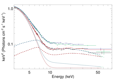
Figure 6.— The unfolded NuSTAR spectra and components of model 5 in $E^{2}\ast f(E)$ representation. Black and red crosses are, respectively, FPMA and FPMB spectra from the non-flare times; green and blue crosses are the flare spectra. The two upper dotted lines exhibit the simpl $\ast$ kerrbb components of the flare and non-flare spectra, while the two lower dashed lines exhibit the reflection components. The reflection component of the flare spectra is stronger than that of the non-flare spectra.

Similar to the fits above, a high folding energy was preferred by model 5. Although we also tested the fits with $E_{\rm fold}$ fixed at 100 keV and the iron abundance left as a free parameter, we only show the spectral fitting with $E_{\rm fold}=500$ keV and Fe/solar=1.5 in Table 3 and Figure 5 because there is only a slight change in the goodness of fit for other values of those parameters. The distance of XTE J1908+094 is thought to be $\sim 2-10$ kpc; thus, $D_{\rm BH}$ was set to be 2 kpc or 10 kpc. The spin and the inclination of kerrbb are linked to those of relconv. Other model parameters were fixed at the default values. We obtained a very small improvement in the fits with the reduced $\rm\chi^{2}$ of 1.06 for 2092 dof. Except for the normalization of the kerrbb model, all model parameters show little changes if $D_{\rm BH}$ was changed from 10 kpc to 2 kpc. Thus, we only show the spectral fitting with $D_{\rm BH}=10$ kpc (see Figure 6). The BH spin can take values in a wide range, from $-0.998$ to $\sim 0.7$. The unabsorbed flux in the 2–12 keV band are $2.7\times 10^{-9}$ erg cm^-2 s^-1 and $2.9\times 10^{-9}$ erg cm^-2 s^-1 for the non-flare and flare spectra, respectively. Using the average flux over the non-flare and flare stages, and assuming a typical $M_{\rm BH}$ of $10~{}M_{\sun}$ and $D_{\rm BH}=(2-10)$ kpc, the source luminosity is $(1-34)\times 10^{36}$ erg s^-1 and the Eddington fraction ($L/L_{\rm Edd}$) is 0.1% – 2.7%. While the upper part of the $L/L_{\rm Edd}$ range would not be unusual for a soft state, the lower part of the range is low for a soft state (e.g., Yu & Yan, 2009), and this may favor a source distance closer to 10 kpc than 2 kpc.

Previously, using the BeppoSAX MECS spectra from the 2002 outburst, Miller et al. (2009) measured the spin of the black hole in XTE J1908+094. The thermal emission was not detected in these spectra; thus, they used the reflection component to constrain the spin and reported a value of $0.75\pm 0.09$. If we fix the spin at 0.75 and set the other parameters to be the same as for model 5, the quality of the spectral fit is still good. Other than the BH mass being larger, the parameters are similar to those of model 5. However, given the large uncertainties in the spin, distance and inclination, it is impossible to constrain $M_{\rm BH}$ with our current data. The inclination measurement is independent of the BH spin that we assume with a value of $\sim 30^{\circ}-40^{\circ}$, similar to $i=45^{\circ}\pm 8^{\circ}$ reported by Miller et al. (2009).

Although these models containing the disk, the power-law (Comptonization) and the reflection components fit the NuSTAR spectra well, upon closer inspection, we find a small bump in the residuals near 8–9 keV (see Figure 5). A similar feature is also observed in some other NuSTAR spectra, such as Cyg X-1 (Tomsick et al., 2014). Adding a Gaussian emission line with $E_{\rm cent}\sim 8.2$ keV and $\sigma\sim 0.3$ keV, the spectral fits are improved with $\Delta{\chi^{2}}\sim 16$, and the key parameters change only slightly. The line feature is likely related to a combination of iron K$\beta$ and nickel emission, neither of which are included in the reflionx_hc model (Walton et al., 2015, in preparation).

4. Discussion

We have presented NuSTAR and Swift observations of XTE J1908+094 during its 2013 outburst. Similar to the two previous outbursts, the source was first detected in the hard state, then went into the soft state and decayed rapidly afterwards. The time interval between the 2013 outburst and the last one is about 10 years, which is much longer than that between the two previous outbursts.

The NuSTAR light curves show a flare of $\sim$ 40 ks duration. Fitting the spectra with the two components combining model of diskbb plus pegpwrlw prior to, during and after the flare, we found the power-law component, rather than the disk component, exhibited major changes during the flare. The power-law was softer and brighter during the flare but seems to be stable in the stages prior to and after the flare. A possible scenario is that there was an injection of high-energy particles (perhaps due to a jet ejection or shocks in the accretion disk) during the flare; thus, the flux of the power-law component increased, and the power-law index varied. If we keep the power-law model constant during the whole observation and add another power-law model in fitting the flare spectrum, the extra emission is found to have a photon index of $\rm\Gamma=2.61\pm 0.04$ with a 3–79 keV flux of $\sim 1.8\times 10^{-10}$ erg cm^-2 s^-1.

Jet ejections are not unusual in Galactic X-ray binaries. Other sources, such as GRS 1915+105 (e.g. Mirabel & Rodríguez, 1994; Fuchs et al., 2003), GRO J1655-40 (e.g. Tingay et al., 1995) and Cygnus X-1 (e.g. Stirling et al., 2001), also show ejection events. There are at least two types of ejections: one is the discrete outflow usually appearing in the hard-to-soft state transition (e.g., Fender et al., 2004; Corbel et al., 2004), and the other is the compact jet occurring in the hard state and disappearing in the hard-to-soft state transition (e.g., Fender et al., 1999; Corbel et al., 2000, 2003). The radio flux of XTE J1908+094 showed a significant increase between 2013 November 5 and November 6 (Rushton et al., 2013b), which was 2–3 days before the NuSTAR observations. Rushton et al. (2013b) and Coriat et al. (2013) suggested that the source ejected some optically thin radio-emitting plasma during the period. In fact, the radio flux peaked during the NuSTAR observation. Also, the radio polarization measurements and the radio spectrum are consistent with the discrete ejection interpretation (Curran et al., 2015). Moreover, we note that radio flares are accompanied by X-ray flares in some X-ray binaries (e.g. Wilms et al., 2007). Based on the facts that the source was in a transition from the hard state to the soft state and the radio flare was apparent, such X-ray ejections would not be surprising. The X-ray flare observed by NuSTAR may have been caused by a discrete ejection.

Although a couple of faint X-ray jets were detected from microquasars a few years after the ejection (e.g., Corbel et al., 2002, 2005), the X-ray emission produced by the plasmoid ejection may not be enough to explain the observed flux of XTE J1908+094. Thus, sudden changes of the temperature or the size of the corona may be another scenario. We used a Comptonization model comptt (Titarchuk, 1994) to replace the power-law model in model 1, and untied different combinations of parameters in the non-flare and flare spectra. If the plasma temperature, $kT_{\rm e}$, and the 3–79 keV flux in units of $\rm 10^{-12}$ erg cm^-2 s^-1, $N_{\rm comp}$, are allowed to be different for the different spectra, we obtain $kT_{\rm e}=500^{+0}_{-140}$ keV and $N_{\rm comp}=377\pm 4$ from the non-flare spectra, and $kT_{\rm e}=306^{+11}_{-77}$ keV and $N_{\rm comp}=526\pm 5$ during the flare, with $\chi^{2}/{\rm dof}=2660.5/2098$; if, instead of the temperature, the plasma optical depth parameter, $\tau$, is allowed to be free, we obtain $\tau=0.030^{+0.028}_{-0.002}$ and $N_{\rm comp}=376\pm 4$ from the non-flare spectra, and $\tau=0.010^{+0.012}_{-0}$ and $N_{\rm comp}=527\pm 5$ during the flare, with $\chi^{2}/{\rm dof}=2658.7/2098$. We note that the ejection might remove material and cause a drop in the optical depth. If the corona is actually part of the jet, such as its base (Markoff et al., 2005), the two explanations that we discuss (an ejection or a change in the coronal properties) might be related.

During the hard state of the 2002 outburst, a broad line feature with an average energy of $E=5.73\pm 0.09$ keV and a line width of $\sigma=1.11\pm 0.31$ keV was observed by Göǧüş et al. (2004). The feature disappeared in the soft state, whereas it reappeared when the source later entered into the hard state. The flux of the line component is strongly linked to that of the power-law component; thus, Göǧüş et al. (2004) suggested that the line feature might be the Fe K$\alpha$ line from the reprocessing of the hard X-ray photons by cooler material close to the central object. In order to search for the line feature over the whole 2013 outburst, we used the same model as Göǧüş et al. (2004) to fit the Swift spectra. However, for most observations, the line feature is not remarkable, and the two component model containing the diskbb and power-law components could also fit the spectra successfully (Figure 2b). This may be due to the lower throughput of Swift/XRT above 6 keV, making the line feature undetectable. Moreover, in several observations of the soft state, the spectra show a possible Fe K$\alpha$ line feature, and this is further confirmed by the NuSTAR observation (see Figure 4 and Figure 5 where there is an iron line and hard X-ray bump). The Gaussian emission line models could fit the line feature, with model 2b (free $N_{\rm H}$) providing a better fit (see Figure 5 and Table 2). If a moderate $N_{\rm H}$ of $2.5\times 10^{22}~{}\rm cm^{-2}$ or $4.3\times 10^{22}~{}\rm cm^{-2}$ is used, $E_{\rm cent}$ agrees with the energy range of iron emission; if $N_{\rm H}$ is allowed to be free, $E_{\rm cent}$ is well below this energy range, in which case the emission line may be redshifted due to the gravitational effect. Regardless of the value of $N_{\rm H}$, the line widths are about 1-2 keV, which are similar to those reported by in’t Zand et al. (2002) and Göǧüş et al. (2004).

The reflection component can also be well fitted by the reflionx_hc model, although the folding energy is not well constrained. As would be expected due to the stronger power-law flux during the flare, the ionization parameter, $\rm\xi$, during the flare is larger than for the non-flare spectra.

Adding a relativistic blurring model (model 4), relconv, provides only a small improvement on the quality of the fit to the spectrum, and the parameters of model 4 and model 5 (replacing the multi-temperature disk-blackbody by the kerrbb model), agree with those of model 3. The reflection covering fractions, calculated from the ratio in 20–40 keV flux between the reflection and the power-law component, are 1.1–2.2 for the non-flare spectra and 1.6–3.9 for the flare spectra based on the different models. We note that the covering fractions are larger than 1, which indicates that the X-ray emission may come from closer to the black hole and the relativistic effects are stronger so that the light is gravitationally bent (Miniutti & Fabian, 2004; Miniutti et al., 2004). Based on the relconv parameters, all possible values for the spin of the black hole ($-0.998$ to 0.998) are allowed when the inner radius is fixed to the ISCO, which means that the spectra may be extremely blurred, with a maximal BH spin, or somewhat less blurred with a retrograde disk or with the inner disk being ionized. Following Dauser et al. (2014), the reflection fraction can give a lower limit on the black hole spin when assuming a lamppost geometry (i.e., a point-like corona above the spin axis of the BH); in that case a covering fraction above 1.6 implies a spin greater than 0.6.

5. Summary and Conclusions

NuSTAR and Swift observed XTE J1908+094 during its 2013 outburst. The Swift monitoring observations show that the source reached the soft state very close to the time that NuSTAR observed the source. A flare with a duration of $\sim 40$ ks appears in the NuSTAR light curve, peaking at $\sim$40% above the non-flare level. When fitting the non-flare and flare spectra with two-component models, consisting of diskbb plus pegpwrlw or diskbb plus comptt, we found that the power-law component (or the Comptonization component), rather than the disk component, went through great changes during the flare. Changes of the corona, including variations of its temperature or its size, or the ejection of hot plasma, are two possible and potentially related scenarios for the flare. A broad iron line feature with $\sigma=1-2$ keV is observed in the NuSTAR spectrum, which motivates a spectral model that combines a thermal disk, a power-law and a reflection component, providing a good fit to the spectrum. Although the broad iron line provides evidence for relativistic blurring of the reflection component, we are not able to constrain the BH spin in the spectral fits, and all possible spin values, from $-0.998$ to $0.998$, are allowed. The strong reflection component requires a covering fraction in excess of 1.0, which may be explained if light bending by the BHs gravitational field enhances the flux incident on the inner disk and suggests a spin larger than 0.6.

References

- Burrows et al. (2005) Burrows, D. N., Hill, J. E., Nousek, J. A., et al. 2005, Space Sci. Rev., 120, 165
- Chaty et al. (2002) Chaty, S., Mignani, R. P., & Israel, G. L. 2002, MNRAS, 337, L23
- Chaty et al. (2006) Chaty, S., Mignani, R. P., & Israel, G. L. 2006, MNRAS, 365, 1387
- Corbel et al. (2000) Corbel, S., Fender, R. P., Tzioumis, A. K., et al. 2000, A&A, 359, 251
- Corbel et al. (2002) Corbel, S., Fender, R. P., Tzioumis, A. K., et al. 2002, Science, 298, 196
- Corbel et al. (2003) Corbel, S., Nowak, M. A., Fender, R. P., Tzioumis, A. K., & Markoff, S. 2003, A&A, 400, 1007
- Corbel et al. (2004) Corbel, S., Fender, R. P., Tomsick, J. A., Tzioumis, A. K., & Tingay, S. 2004, ApJ, 617, 1272
- Corbel et al. (2005) Corbel, S., Kaaret, P., Fender, R. P., et al. 2005, ApJ, 632, 504
- Coriat et al. (2013) Coriat, M., Tzioumis, T., Corbel, S., & Fender, R. 2013, The Astronomer’s Telegram, 5575, 1
- Curran et al. (2015) Curran, P. A., Miller-Jones, J. C. A., Rushton, A. P., et al. 2015, arXiv:1506.01141
- Dauser et al. (2010) Dauser, T., Wilms, J., Reynolds, C. S., & Brenneman, L. W. 2010, MNRAS, 409, 1534
- Dauser et al. (2014) Dauser, T., García, J., Parker, M. L., Fabian, A. C., & Wilms, J. 2014, MNRAS, 444, L100
- Fender et al. (1999) Fender, R., Corbel, S., Tzioumis, T., et al. 1999, ApJ, 519, L165
- Fender et al. (2004) Fender, R. P., Belloni, T. M., & Gallo, E. 2004, MNRAS, 355, 1105
- Feroci et al. (2002) Feroci, M., Reboa, L., & BEPPOSAX Team 2002, IAU Circ., 7861, 2
- Fuchs et al. (2003) Fuchs, Y., Rodriguez, J., Mirabel, I. F., et al. 2003, A&A, 409, L35
- Göǧüş et al. (2004) Göǧüş, E., Finger, M. H., Kouveliotou, C., et al. 2004, ApJ, 609, 977
- Harrison et al. (2013) Harrison, F. A., Craig, W. W., Christensen, F. E., et al. 2013, ApJ, 770, 103
- in’t Zand et al. (2002) in’t Zand, J. J. M., Miller, J. M., Oosterbroek, T., & Parmar, A. N. 2002, A&A, 394, 553
- Jonker et al. (2004) Jonker, P. G., Gallo, E., Dhawan, V., et al. 2004, MNRAS, 351, 1359
- Krimm et al. (2013a) Krimm, H. A., Barthelmy, S. D., Baumgartner, W., et al. 2013, The Astronomer’s Telegram, 5523, 1
- Krimm et al. (2013b) Krimm, H. A., Kennea, J. A., & Holland, S. T. 2013, The Astronomer’s Telegram, 5529, 1
- Li et al. (2005) Li, L.-X., Zimmerman, E. R., Narayan, R., & McClintock, J. E. 2005, ApJS, 157, 335
- Lightman & White (1988) Lightman, A. P., & White, T. R. 1988, ApJ, 335, 57
- Markoff et al. (2005) Markoff, S., Nowak, M. A., & Wilms, J. 2005, ApJ, 635, 1203
- McClintock & Remillard (2006) McClintock, J. E., & Remillard, R. A. 2006, Compact stellar X-ray sources, 157
- Miller (2007) Miller, J. M. 2007, ARA&A, 45, 441
- Miller et al. (2009) Miller, J. M., Reynolds, C. S., Fabian, A. C., Miniutti, G., & Gallo, L. C. 2009, ApJ, 697, 900
- Miller-Jones et al. (2013) Miller-Jones, J. C. A., Sivakoff, G. R., & Krimm, H. A. 2013, The Astronomer’s Telegram, 5530, 1
- Miniutti & Fabian (2004) Miniutti, G., & Fabian, A. C. 2004, MNRAS, 349, 1435
- Miniutti et al. (2004) Miniutti, G., Fabian, A. C., & Miller, J. M. 2004, MNRAS, 351, 466
- Mirabel & Rodríguez (1994) Mirabel, I. F., & Rodríguez, L. F. 1994, Nature, 371, 46
- Negoro et al. (2013) Negoro, H., Suzuki, K., Ueno, J. S. S., et al. 2013, The Astronomer’s Telegram, 5549, 1
- Reynolds & Nowak (2003) Reynolds, C. S., & Nowak, M. A. 2003, Phys. Rep., 377, 389
- Ross et al. (1999) Ross, R. R., Fabian, A. C., & Young, A. J. 1999, MNRAS, 306, 461
- Ross & Fabian (2005) Ross, R. R., & Fabian, A. C. 2005, MNRAS, 358, 211
- Rupen et al. (2002) Rupen, M. P., Dhawan, V., & Mioduszewski, A. J. 2002, IAU Circ., 7874, 1
- Rushton et al. (2013a) Rushton, A. P., Fender, R., Anderson, G., et al. 2013, The Astronomer’s Telegram, 5532, 1
- Rushton et al. (2013b) Rushton, A. P., Fender, R., Anderson, G., et al. 2013, The Astronomer’s Telegram, 5551, 1
- Titarchuk (1994) Titarchuk, L. 1994, ApJ, 434, 570
- Steiner et al. (2009) Steiner, J. F., Narayan, R., McClintock, J. E., & Ebisawa, K. 2009, PASP, 121, 1279
- Stirling et al. (2001) Stirling, A. M., Spencer, R. E., de la Force, C. J., et al. 2001, MNRAS, 327, 1273
- Tingay et al. (1995) Tingay, S. J., Jauncey, D. L., Preston, R. A., et al. 1995, Nature, 374, 141
- Tomsick et al. (2014) Tomsick, J. A., Nowak, M. A., Parker, M., et al. 2014, ApJ, 780, 78
- Walton et al. (2015, in preparation) Walton, D. J., et al. 2015, in preparation
- Wilms et al. (2000) Wilms, J., Allen, A., & McCray, R. 2000, ApJ, 542, 914
- Wilms et al. (2007) Wilms, J., Pottschmidt, K., Pooley, G. G., et al. 2007, ApJ, 663, L97
- Woods et al. (2002) Woods, P. M., Kouveliotou, C., Finger, M. H., et al. 2002, IAU Circ., 7856, 1
- Yu & Yan (2009) Yu, W., & Yan, Z. 2009, ApJ, 701, 1940