Limiting Energy Loss Distributions for Multiphoton Channeling Radiation

Abstract

Recent results in the theory of multiphoton spectra for coherent radiation sources are overviewed, with the emphasis on channeling radiation. For the latter case, the importance of the order of resummation and averaging is illustrated. Limiting shapes of multiphoton spectra at high intensity are discussed for different channeling regimes. In some spectral regions, there emerges an approximate correspondence between the radiative energy loss and the electron integrals of motion.

1 Introduction

Ultrarelativistic electrons moving periodically in coherent radiation sources produce fairly monochromatic radiation. The intensity of this radiation is proportional to the length of the periodic or confining structure, and if it is sufficiently high, the electron is likely to emit several photons during its passage. The problem of multiple photon emission per electron plays significant role for crystalline radiators with thickness $\gtrsim 1\%X_{0}$ [1], Compton sources with optical laser pulse energy densities $\gtrsim 1\frac{\text{J}}{\mu\text{m}^{2}}\frac{E_{e}}{\text{GeV}}$ [2, 3], synchrotron radiation [4], undulators with the number of periods $\gtrsim 10^{2}$ [5]. At that, multiple photon emissions from different electrons can be discriminated by means of coincidences between detectors, except in cases when the electron beam density is very high (e.g., in SASE FELs), and so only the problem of photon pileup from one electron remains.

Physically, the multiple photon emission from an electron in a strong electromagnetic field may be viewed as a kind of electromagnetic showering. It greatly simplifies if, as is typical for many coherent radiation sources, energies of emitted photons are much smaller than the electron energy:

$$\omega\ll E_{e}.$$ (1)

Then, in the first approximation, it is permissible to count only photons stemming directly from the classical current generated by the initial electron, and neglect $e^{+}e^{-}$ pairs produced by those photons downstream.

For different experiments, though, the quantities of interest under conditions of multiple photon emission may differ. For instance, in synchrotrons one is concerned with lag fluctuations of an electron accelerated by the running wave, in FELs – electron bunching, in Compton sources – electron energy straggling before its last interaction with a photon yielding the observed gamma-quantum. For coherent radiation in oriented crystals, one does not really care about the spent electron, but instead, measurements of the radiation are usually carried out with calorimeters, and are restricted to spectra integrated over (relativistically small) emission angles. Then, only the aggregate energy of all the nearly forward moving photons from one electron is measured. In the present article, we will discuss the latter case.

2 Resummation technique and its alternatives

As was mentioned above, the possibility of photon pileup in the calorimeter causes significant deviation of the multiphoton probability (i.e., the radiative energy loss) spectrum $dw/d\omega$ from the single-photon spectrum $\frac{dw_{1}}{d\omega_{1}}=\frac{1}{\omega_{1}}\frac{dI_{\text{cl}}}{d\omega_{1}}$ predicted by classical electrodynamics, in spite of condition (1). Nonetheless, a multiphoton spectrum can be deduced from the corresponding single-photon one, as is described below.

Technically, the situation is the simplest when one’s knowledge of initial conditions for the electron and the target is sufficient for completely specifying the electron’s trajectory. Then, presuming that photons exert negligible back action on the electron, their probability distribution obeys Poisson statistics [6, 7]

$$\frac{dW_{n}}{d\omega_{1}\ldots d\omega_{n}}=W_{0}\frac{1}{n!}\frac{dw_{1}}{d\omega_{1}}\ldots\frac{dw_{1}}{d\omega_{n}},$$ (2)

where $n$ is the number of emitted photons, $W_{0}=e^{-\int_{0}^{\infty}d\omega_{1}\frac{dw_{1}}{d\omega_{1}}}$ is the photon non-emission probability, and factor $1/n!$ accounts for photon equivalence. It is important to note, though, that the statistical independence of photon emission events does not imply that they occur sequentially in time. For instance, in a coherent state of the quantized electromagnetic field (a closest counterpart to a classical electromagnetic field) [6], there is a quantum superposition rather than mere statistical mixture of photon number states, which is indicative of their simultaneous generation.

To derive from (2) the radiation spectrum measured by a calorimeter, one must integrate the fully differential spectrum for any definite number of emitted photons over their entire phase space, under the restriction of the sum of photon energies to a certain value $\omega$, and then sum over photon multiplicities:

$$\frac{dw}{d\omega}=\sum_{n=1}^{\infty}\int d\omega_{1}\ldots d\omega_{n}\frac{dW_{n}}{d\omega_{1}\ldots d\omega_{n}}\delta\left(\omega-\sum_{k=1}^{n}\omega_{k}\right).$$ (3)

Series (3) can further be resummed to all orders, by Laplace transforming it, whereafter it exponentiates, and then can be transformed back to the $\omega$ variable:

$$\frac{dw}{d\omega}=\frac{1}{2\pi i}\int_{c-i\infty}^{c+i\infty}dse^{s\omega+\int_{0}^{\infty}d\omega_{1}\frac{dw_{1}}{d\omega_{1}}\left(e^{-s\omega_{1}}-1\right)}-W_{0}\delta(\omega).$$ (4)

The integration contour in (4) is flexible in the complex $s$ plane, but the integrand is not the only possible one, too: The upper limit of the integral in the exponent can be actually set equal to any value greater than $\omega$, which can be expedient when dealing with incoherent radiation component [8]. For single-photon spectra with a relatively sharp upper end $\omega_{0}\ll E_{e}$, it is usually sufficient to let the upper integration limit equal to $\omega_{0}$.

The practical benefit of the exponentiation is that it reduces the number of integrals to be handled. If one attempts instead to calculate termwise the probabilities of emission of a certain number of photons via Eg. (3), computation of the multiple integrals even numerically quickly becomes prohibitive. Sometimes, nonetheless, such multiple integrals are computed by Monte-Carlo – see, e.g., Ref. 2 of [3].

An approach alternative to (4) is to view $dw/d\omega$ as a solution of an integro-differential equation with the single-photon spectrum playing the role of its kernel. Specifically, presuming that $dw_{1}/d\omega_{1}$ is proportional to the target thickness $L$, one can formally derive the standard transport equation

$$\frac{\partial}{\partial L}\Pi(E_{e}-\omega)=\int_{0}^{\infty}d\omega_{1}\frac{\partial}{\partial L}\frac{dw_{1}}{d\omega_{1}}\left[\Pi(E_{e}-\omega+\omega_{1})-\Pi(E_{e}-\omega)\right]$$ (5)

holding for the electron energy distribution function

$$\Pi(E_{e}-\omega)=\frac{dw}{d\omega}+W_{0}(L)\delta(\omega).$$ (6)

Equation (5) might also serve as an alternative justification for the $1/n!$ factor in (2), by virtue of the identity

$$\frac{\partial}{\partial L}\int d\omega_{1}\ldots d\omega_{n}\prod_{k=0}^{n}\frac{dw_{1}}{d\omega_{k}}\delta\left(\omega-\sum_{k=1}^{n}\omega_{k}\right)\qquad\qquad$$

$$=n\int d\omega_{1}\ldots d\omega_{n}\prod_{k=0}^{n-1}\frac{dw_{1}}{d\omega_{k}}\frac{\partial}{\partial L}\frac{dw_{1}}{d\omega_{n}}\delta\left(\omega-\sum_{k=1}^{n}\omega_{k}\right),$$

should it not be the fact that each photon may actually be coherently generated along a large length, simultaneously with formation of other photons.

Another popular approach for computing multiphoton emission probabilities during semi-classical electron passage is to divide the trajectory into several pieces, the interference of radiation from which is expected to be negligible, and define a probabilistic process of photon emission or non-emission on the junctions. It also permits taking into account incoherent scattering during radiation, and other accompanying processes. That approach led to construction of Monte Carlo simulators widely used in modern practice [1, 11, 12, 13]. At the present state of the art, such generators usually employ kernels of generation of only one photon, which is subsequently iterated – as well as in the resummation approach described above.

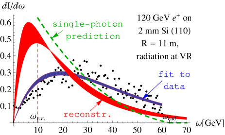
Figure 1: Simplified reconstruction of the single-photon spectrum from multiphoton one, for radiation at volume reflection. Points, data of [14] for a 2 mm crystal bent to radius 11 m. Blue band, fit of $\omega\frac{dw}{d\omega}=A\omega e^{-\alpha\omega}$ to experimental data, the adjusted parameters being $A=0.042\pm 0.003\text{ GeV}^{-1}$ and $\alpha=0.053\pm 0.002\text{ GeV}^{-1}$. Red band, the reconstructed single-photon spectrum $\omega_{1}\frac{dw_{1}}{d\omega_{1}}=e^{-\alpha\omega_{1}}-e^{-\frac{\alpha}{1-A/\alpha}\omega_{1}}$. Dashed green curve, prediction for the single-photon spectrum of coherent bremsstrahlung in a bent crystal [15].

Adopting an analogy with high-energy physics, one can envisage further development of simulators to include non-factorized evaluation of two-photon emission along with the appropriate account of virtual radiative corrections, simulation of a shower including coherent photon emission from $e^{+}e^{-}$ pairs, etc. But for qualitative analysis, the resummation method within the region of its validity is advantageous by its simplicity. Below, we will confine ourselves to discussing a few examples of its application.

Before we proceed, it is worth pointing out that in case when there are no random parameters on which the spectrum significantly depends and which are to be averaged over, relation (4) can be inverted to reconstruct the single-photon spectrum from the observed multiphoton one [8]. In Fig. 1 we show an example where a single-photon spectrum of radiation at volume reflection was reconstructed (in a simplified fashion) from the experimental data. Without taking multiphoton effects into account, the agreement between the experiment and the theory leaves much to be desired [16], but after the reconstruction it becomes acceptable. Needless to say, the reconstruction procedure is expected to be efficient only if the radiation intensity (photon multiplicity) is not too high. In what follows, we will discuss cases of high intensity and show that the corresponding spectra may have diverse shapes depending on the physical conditions.

3 High-intensity limit and the departures from Gaussianity

For pure coherent radiation, typically characterized by an edgy single-photon spectrum, multiple photon emission imitates the appearance of higher spectral harmonics. With the increase of the radiation intensity, such quasi-harmonics proliferate and coalesce into universal forms depending on just few parameters. For a definite and smooth electron trajectory, the (central) limiting form of the multiphoton spectrum is a Gaussian, as one would expect:

$$\frac{dw_{\text{c}}}{d\omega}\simeq\frac{1}{\sqrt{2\pi\overline{\omega_{1}^{2}}}}\exp\left[-\frac{(\omega-\overline{\omega_{1}})^{2}}{2\overline{\omega_{1}^{2}}}\right].$$ (7)

The corresponding regime may be physically categorized as a normal random walk. At large $\omega$ beyond the maximum, the spectrum decreases closer to an ordinary exponential rather than Gaussian law [8]. That can be interpreted in terms of a maximal-step walk, at which the probability is a product of probabilities for each maximal step, the number of steps being $\sim{\omega/\omega_{0}}$.

A correction to (7) breaking the scaling was obtained in [8]. It engages the third spectral moment related to skewedness. Besides rendering the asymmetry to the spectrum, it slightly redshifts its maximum.

Another source of departure from the Gaussianity, even in the absence of dependence of the underlying single-photon spectrum on external parameters, is the possible infinity of the spectral moments defining the Gaussian. For instance, in the case of coherent bremsstrahlung (at a highly over-barrier electron motion), the dependence on electron impact parameters is negligible, but yet there is an incoherent radiation component described by Bethe-Heitler single-photon spectrum $\frac{dw_{1}}{d\omega_{1}}=\frac{a}{\omega_{1}}$, for which the spectral moments diverge in the ultraviolet (or more precisely, are dominated by the upper endpoint $\omega\to E_{e}$, around which our soft-photon resummation approach breaks down). That leads to a modification of the limiting spectrum shape by a power-law tail persisting at high $\omega$. The tail, however, does not override the whole spectrum, whose maximum is still mainly determined by the coherent part of the spectrum and its convergent first moments. Therefore, the diffusion regime may be regarded as weakly anomalous, and the resulting distribution as intermediate between Gaussian and Lèvy [8]. Within our framework, the anomaly must keep weak, i.e. its index $a=L/X_{0}$ must remain small, or else the shower will not be dominated by soft photons.

4 Channeling radiation: the impact of initial state averaging

Our formulation so far held for radiation from a completely prescribed electromagnetic current. Next, it is important to ask what happens in case of channeling radiation, when the radiation intensity, and therewith the photon multiplicity, strongly depends on the electron/positron oscillation amplitude in the channel, in turn depending on the electron impact parameter and the angle of entrance to the crystal. Clearly, in the latter case the multiphoton spectrum must be duly averaged over the initial electron beam.

An important point here is that the averaging must be carried out after the resummation, and this order of operations is significant under the condition of high photon multiplicity. Clearly, in Eq. (4), the average of an exponential does not reduce to an exponentiated average,

$$\left\langle e^{\int_{0}^{\infty}d\omega_{1}\frac{dw_{1}}{d\omega_{1}}\left(e^{-s\omega_{1}}-1\right)}\right\rangle\neq e^{\int_{0}^{\infty}d\omega_{1}\left\langle\frac{dw_{1}}{d\omega_{1}}\right\rangle\left(e^{-s\omega_{1}}-1\right)}.$$ (8)

Similarly, in Eq. (5),

$$\left\langle\Pi(E_{e}-\omega+\omega_{1})\frac{\partial}{\partial L}\frac{dw_{1}}{d\omega_{1}}\right\rangle\neq\left\langle\Pi(E_{e}-\omega+\omega_{1})\right\rangle\left\langle\frac{\partial}{\partial L}\frac{dw_{1}}{d\omega_{1}}\right\rangle,$$ (9)

invalidating the transport equation for the averaged distribution function with the averaged kernel. In fact, such equations were heuristically used in the literature both for overbarrier motion and for channeling conditions. At that, sometimes they involved adjustable parameters to be determined from fits to observable spectra. However, since the fraction of particles near the bottom of the channel radiates weakly, but contributes to the total number of passed electrons strongly, estimates even of the mean photon multiplicity per electron based on kinetic equation with an averaged kernel can be deceptive.

A related issue is that the knowledge of an averaged single-photon spectrum without detailing its dependence on the electron initial conditions is insufficient for deducing the (averaged) multiphoton spectrum. Indeed, the averaged single-photon spectrum $\left\langle\frac{\partial}{\partial L}\frac{dw_{1}}{d\omega_{1}}\right\rangle$ depends on a single variable $\omega_{1}$, whereas the averaged multiphoton spectrum nontrivially depends on two variables: $\omega$ and the target thickness $L$, while the dependence on $L$ is intertwined with the dependence on the electron initial conditions. It should be stressed yet that the dependence of the radiation on initial conditions must include both the incidence angle and the impact parameter. Whereas the dependence on the former is measurable in principle (cf., e.g., [17]), the dependence on the latter is not (there are no relativistic beams of angstrom transverse size), and thus inevitably must be modeled theoretically.

Let us now discuss typical high-intensity channeling radiation spectrum shapes, for different types of confining wells, and for simplicity neglecting dechanneling.

4.1 Positron channeling

The averaged multiphoton spectrum is most easily tractable for channeling of positrons, when the continuous potential of aligned axes or planes may be regarded as approximately parabolic in the entire channel (as is known to be the case for silicon crystals in orientation $(110)$, $\left\langle 111\right\rangle$, or $\left\langle 100\right\rangle$). Then, the particle trajectories in the channels are given by harmonic curves, and the single-photon radiation spectrum is explicitly expressible, too. It is proportional to the amplitude squared of the transverse motion, and therefore to the electron transverse energy $E_{\perp}$, whereas the differential of the phase space over which the initial conditions are uniformly distributed can be written as $dE_{\perp}^{\mathcal{D}}$, with $\mathcal{D}$ the channeling well dimensionality:

$$\left\langle\ldots\right\rangle=\frac{1}{E_{\perp\max}^{\mathcal{D}}}\int_{0}^{E_{\perp\max}}dE_{\perp}^{\mathcal{D}}\ldots=\mathcal{D}\int_{0}^{1}d\xi\xi^{\mathcal{D}-1}\ldots.$$ (10)

Here value $\mathcal{D}=2$ corresponds to capture to axial channeling from a beam with angular divergence $>\theta_{c}$, $\mathcal{D}=1$ – to capture to planar channeling from a beam with angular divergence $>\theta_{c}$, or to axial channeling from a beam co-aligned with the axis and having divergence $\ll\theta_{c}$, and $\mathcal{D}=1/2$ corresponds to planar channeling from a perfectly aligned beam with divergence $\ll\theta_{c}$.

The analysis of the contour integral (4) averaged in this way is still rather involved, but at high intensity, one can view the spectrum just as a superposition of Gaussians. Inserting (7) into Eq. (10) then yields

$$\frac{dw_{e^{+}}}{d\omega}=\frac{\mathcal{D}}{\sqrt{2\pi\overline{\omega_{1}^{2}}(E_{\perp\max})}}\int_{0}^{1}d\xi\xi^{\mathcal{D}-3/2}\exp\left\{-\frac{\left[\omega-\xi\overline{\omega_{1}}(E_{\perp\max})\right]^{2}}{2\xi\overline{\omega_{1}^{2}}(E_{\perp\max})}\right\}.$$ (11)

The latter integral can be expressed in terms of error functions, but we will restrict ourselves to elucidating its qualitative behavior.

At $\omega<\overline{\omega_{1}}(E_{\perp\max})-\Delta$, with $\Delta\gg\sqrt{\overline{\omega_{1}^{2}}(E_{\perp\max})}$, the maximum of the integrand at $\xi\approx{\omega}/{\overline{\omega_{1}}(E_{\perp\max})}$ falls well within the integration interval, thereby giving the dominant contribution to the integral. Neglecting contributions from the endpoints leads to the result

$$\frac{dw_{e^{+}}}{d\omega}\underset{\omega<\overline{\omega_{1}}(E_{\perp\max})-\Delta}{\simeq}\frac{\mathcal{D}}{\omega}\left[\frac{\omega}{\overline{\omega_{1}}(E_{\perp\max})}\right]^{\mathcal{D}}.$$ (12)

It is independent of the variance $\overline{\omega_{1}^{2}}(E_{\perp\max})$, and might be obtained by replacing partial Gaussians (including their pre-exponential factor) in (11) by the infinitesimally narrow distribution

$$\delta\left[\omega-\xi\overline{\omega_{1}}(E_{\perp\max})\right].$$

That also demonstrates the existence of an approximate one-to-one correspondence between $\omega$ and the transverse energy of the positron quantified by the ratio $\xi=E_{\perp}/E_{\perp\max}$.

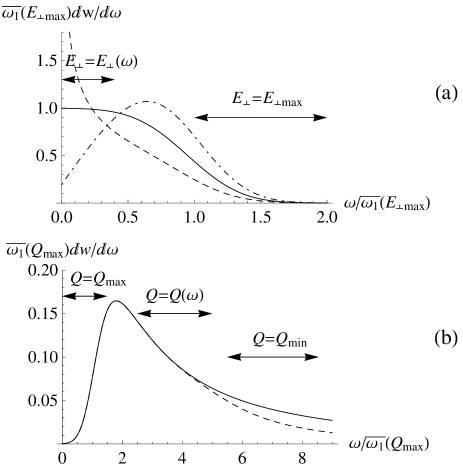
Figure 2: (a) High-intensity approximations (11) for multiphoton channeling radiation from positrons, for $\langle n\rangle\mathcal{D}=n_{\max}\sim\overline{\omega_{1}}^{2}(E_{\perp\max})/\overline{\omega_{1}^{2}}(E_{\perp\max})=10$. Dashed curve, planar channeling radiation from monokinetic beam, $\mathcal{D}=1/2$. Solid curve, planar channeling radiation, $\mathcal{D}=1$. Dot-dashed curve, axial channeling radiation, $\mathcal{D}=2$. (b) High-intensity approximations for multiphoton channeling radiation from axially channeled electrons. Solid curve, Eq. (4.2), for $\overline{\omega_{1}}^{2}(T_{\max},\Lambda_{\max})/\overline{\omega_{1}^{2}}(T_{\max},\Lambda_{\max})=10$. Dashed curve, the same with a lower cutoff $\lambda_{\min}=\tau_{\min}=0.2$.

On the contrary, beyond the break, the integrand exponentially increases throughout the integration interval. Therefore, the main contribution to the integral comes from a vicinity of the endpoint $\xi=1$, around which the $\xi$-dependence of the exponent can be linearized, whereas $\xi^{\mathcal{D}-3/2}$ be put to unity, giving

$$\frac{dw_{e^{+}}}{d\omega}\underset{\omega>\overline{\omega_{1}}(E_{\perp\max})+\Delta}{\simeq}\frac{\mathcal{D}}{\sqrt{\pi}}\frac{\sqrt{2\overline{\omega_{1}^{2}}(E_{\perp\max})}}{\omega^{2}-\overline{\omega_{1}}^{2}(E_{\perp\max})}e^{-\frac{\left[\omega-\overline{\omega_{1}}(E_{\perp\max})\right]^{2}}{2\overline{\omega_{1}^{2}}(E_{\perp\max})}}.$$ (13)

Examples of behavior of function (11) are shown in Fig. 2(a). The spectra strongly depend on the value of $\mathcal{D}$, especially at low $\omega$, in accord with asymptotics (12). That illustrates the profound effect of the averaging on multiphoton channeling radiation spectra.

4.2 Axial channeling of electrons

Compared to positrons, channeling of electrons, generally, is affected by dechanneling stronger, because electrons are attracted to atomic nuclei, and thus may enter regions of strong scattering. For axial orientation of the crystal, though, electrons can orbit around positively charged atomic strings, and thus keep on distance from nuclear vicinities. The approximate axial symmetry of a string alone, without introducing oversimplified assumptions about the $r_{\perp}$ dependence, does not yet permit explicitly expressing electron trajectories and therefrom the radiation spectra. Nonetheless, qualitative analysis is feasible for a potential modeled by a pure logarithmic function with a sharp cutoff at large radial distance $r_{\perp}$:

$$V(r_{\perp})=V_{0}\ln\frac{r_{\perp}}{r_{a}}\vartheta(r_{a}-r_{\perp}),\qquad r_{\perp}<r_{a}.$$ (14)

The motion of electrons in potential (14) is determined by two integrals of motion: transverse energy $E_{\perp}$ and projection $\Lambda$ of the angular momentum on the string direction. Estimates of first moments of the single-photon spectrum in a crystal of definite thickness give:

$$\overline{\omega_{1}}=\int_{0}^{\infty}d\omega_{1}\frac{dI}{d\omega_{1}}\propto\frac{1}{\Lambda T},$$ (15)

and

$$\overline{\omega^{2}_{1}}=\int_{0}^{\infty}d\omega_{1}\omega_{1}\frac{dI}{d\omega_{1}}\sim\frac{4\pi\gamma^{2}}{T}\overline{\omega_{1}}\propto\frac{1}{\Lambda T^{2}},$$ (16)

where $T$ is the period of the radial motion, exponentially depending on $E_{\perp}/V_{0}$, and relatively weakly dependent on $\Lambda$. Both spectral moments blow up as $T\to 0$ or $\Lambda\to 0$, i.e., when the electron passes close to the singularity of the continuous potential.

The element of the uniformly populated phase space can be expressed in terms of $T$, $\Lambda$, as well:

$$d^{2}r_{\perp}d^{2}p_{\perp}\propto TdE_{\perp}d\Lambda\approx V_{0}dTd\Lambda,$$ (17)

and the region accessible to channeling (subject to condition $E_{\perp}<0$) is

$$0\leq\lambda=\frac{|\Lambda|}{\Lambda_{\max}}\leq\tau=\frac{T}{T_{\max}}\leq 1,$$

where $T_{\max}\approx 3r_{a}\sqrt{E_{e}/V_{0}}$, $\Lambda_{\max}=r_{a}\sqrt{E_{e}V_{0}/e}$. Ultimately, the averaged multiphoton spectrum assumes the form

$$\frac{dw_{e^{-}\text{ax}}}{d\omega}=\frac{2}{\sqrt{2\pi\overline{\omega_{1}^{2}}(Q_{\max})}}\qquad\qquad\qquad\qquad\qquad\quad$$

$$\times\int_{0}^{1}d\tau\tau\int_{0}^{\tau}d\lambda\sqrt{\lambda}\exp\left\{-\frac{\left[\omega\lambda\tau-\overline{\omega_{1}}(Q_{\max})\right]^{2}}{2\lambda\overline{\omega_{1}^{2}}(Q_{\max})}\right\},$$ (18)

with $Q_{\max}=T_{\max}\Lambda_{\max}$. Again, we restrict ourselves to qualitative analysis of integral (4.2).

At $\omega<\overline{\omega_{1}}(Q_{\max})-\Delta$, $\Delta\gg\sqrt{\overline{\omega_{1}^{2}}(Q_{\max})}$, the maximum of the integrand at $\lambda\tau={\overline{\omega_{1}}(Q_{\max})}/{\omega}$ is beyond the integration domain. Therefore, the main contribution comes from the endpoint $\lambda=\tau=1$, and generally, the integral is exponentially small:

$$\frac{dw_{e^{-}\text{ax}}}{d\omega}\!\!\underset{\omega<\overline{\omega_{1}}(Q_{\max})-\Delta}{\simeq}\!\!\sqrt{\frac{2}{\pi}}\frac{2\overline{\omega_{1}^{2}}^{3/2}(Q_{\max})}{\left[\overline{\omega_{1}}^{2}(Q_{\max})-\omega^{2}\right]\left[\overline{\omega_{1}}(Q_{\max})+\omega\right]}$$

$$\times\exp\left\{-\frac{\left[\omega-\overline{\omega_{1}}(Q_{\max})\right]^{2}}{2\overline{\omega_{1}^{2}}(Q_{\max})}\right\}.\qquad\quad$$ (19)

On the contrary, at $\omega>\overline{\omega_{1}}(Q_{\max})+\Delta$, the maximum of the integrand falls well within the integration domain. Neglecting the endpoint contributions, or simply inserting

$$\delta\left[\omega-\overline{\omega_{1}}(Q_{\max})/\lambda\tau\right]$$ (20)

in place of the partial Gaussians, the asymptotics of the multiphoton spectrum derives as

$$\frac{dw_{e^{-}\text{ax}}}{d\omega}\underset{\omega>\overline{\omega_{1}}(Q_{\max})+\Delta}{\simeq}\frac{\overline{\omega_{1}}(Q_{\max})}{\omega^{2}}\ln\frac{\omega}{\overline{\omega_{1}}(Q_{\max})}.$$ (21)

The corresponding mean energy loss $\int_{0}^{\infty}d\omega\omega\frac{dw_{e^{-}\text{ax}}}{d\omega}$ diverges in the ultraviolet as a double logarithm, in accordance with the double logarithmic divergence of the single-photon average mean energy loss, cf. Eq. (15).

The delta function (20) implies that a correspondence between $\omega$ and the integrals of motion holds for electron axial channeling radiation, as well. But in contrast to radiation from channeled positrons, the correspondence here takes place at the outer slope of the spectrum [see Fig. 2(b)]. Yet, since there are two integrals of motion, the correspondence of $\omega$ with them is no longer one-to-one, unless one refers to the special integral of motion $Q=T\Lambda\propto e^{E_{\perp}/V_{0}}\Lambda$.

Experimentally measured multiphoton axial channeling radiation spectra [17, 18] decrease considerably faster than by power law (21). That must be attributed to the crudeness of our model (14) and the physical finiteness of $\left\langle\overline{\omega_{1}}\right\rangle$ due to the smearing of the string potential at low $r_{\perp}$ through thermal and quantum vibrations. The simplest way to take all that into account is to introduce a lower cutoff $\lambda_{\min}=\tau_{\min}$ into integrals (4.2), which leads to an exponentially decreasing spectrum [see Fig. 2(b), dashed curve]. The beginning of the exponential suppression region depends on the value of the cutoff parameter and therethrough on the crystal temperature.

5 Limitations and challenges

The intrinsic simplicity of the soft photon resummation procedure makes it a useful tool in various physical situations, predicting generation of higher quasi-harmonics at moderate intensity (as discussed in [8]) and the existence of a set of limiting distributions at high intensity, depending on the shape of the confining well, yet yielding in certain spectral regions approximate correspondence between the radiative loss $\omega$ and one of the integrals of motion of the channeled particle.

At the same time, the resummation method has its limitations and is unable to cover, e.g., the case when a considerable part of the spectrum concentrates near the kinematic edge $\omega=E_{e}$ [19]. Also, even in the domain of applicability of the soft photon approximation (1), one may wish to evaluate higher order corrections in $\omega/E_{e}$, e.g., in order to account for degradation of $E_{e}$ stipulating additional broadening and redshift of the multiphoton spectra [20], or to describe the effect of electron beam bunching in FELs [5].

For the specific problem of channeling radiation, there arise additional issues. First is the need for knowledge of not only the averaged single-photon spectrum, which might be measured at a sufficiently small crystal thickness, but also of the dependence of the radiation spectrum on electron entrance parameters. That can be illustrated, e.g., by the variance of the multiphoton spectrum about the mean value, for positron channeling in a harmonic well discussed in Sec. 4.1:

$$\left\langle\overline{(\omega-\left\langle\overline{\omega}\right\rangle)^{2}}\right\rangle=\left\langle\overline{\omega^{2}_{1}}\right\rangle+\left\langle\overline{\omega_{1}}\right\rangle^{2}\frac{1}{\mathcal{D}(\mathcal{D}+2)}.$$ (22)

Due to the second term, it depends on the target thickness nonlinearly, yet involving a dependence on the value of $\mathcal{D}$, which in turn depends on the shape of the well. Also, the existence of a correspondence in some spectral regions between $\omega$ and the particle integrals of motion implies that not all the values of integrals of motion contribute at a given $\omega$, in contrast to the case of the averaged single-photon spectrum.

Further complications emerge because in the presence of dechanneling, relative contributions of different integrals of motion can attenuate differently. The corresponding factors thus must be introduced into integrals (11), (4.2). Thirdly, the dechanneled particles contribute to the radiation spectrum, as well, although in a somewhat harder spectral region. That demands inclusion of their contribution to the multiphoton spectrum, too. On the other hand, studying multiphoton radiation spectra under such conditions may offer deeper insight into the complex dynamics of channeling.

References

- [1] J. Bak et al., Nucl. Phys. B 254 (1985) 491; ibid. 302 (1988) 525.
- [2] V. Telnov, NIM A 355 (1995) 3.
- [3] A. Di Piazza, C. Müller, K.Z. Hatsagortsyan, and C.H. Keitel. Rev. Mod. Phys. 84 (2012) 1177; A. Di Piazza, K.Z. Hatsagortsyan, and C.H. Keitel. Phys. Rev. Lett. 105 (2010) 220403.
- [4] A.W. Chao and M. Tigner (eds.), Handbook of Accelerator Physics and Engineering, World Scientific, Singapore, 2002.
- [5] A. Friedman et al., Rev. Mod. Phys. 60 (1988) 471.
- [6] R.J. Glauber, Phys. Rev. 84 (1963) 395; A.I. Akhiezer and V.B. Berestetskii, Quantum Electrodynamics, Nauka, Moscow, 1981 (in Russian).
- [7] V.N. Baier and V.M. Katkov, Phys. Rev. D 59 (1999) 056003.
- [8] M.V. Bondarenco, Phys. Rev. D 90 (2014) 013019.
- [9] M.V. Bondarenco, J. Phys. Conf. Ser. 517 (2014) 012027.
- [10] G. Parisi and R. Petronzio, Nucl. Phys. B 154 (1979) 427; J. Collins, D. Soper, and G. Sterman, Nucl. Phys. B 250 (1985) 199.
- [11] V.N. Baier, V.M. Katkov, and V.M. Strakhovenko, Sov. Phys. Usp. 32 (1989) 972.
- [12] X. Artru, NIM B 48 (1990) 278.
- [13] V. Guidi, L. Bandiera and V. Tikhomirov, Phys. Rev. A 86 (2012) 042903.
- [14] D. Lietti et al., NIM B 283 (2012) 84.
- [15] M.V. Bondarenco, Phys. Rev. A 81 (2010) 052903.
- [16] M.V. Bondarenco, J. Phys. Conf. Ser. 236 (2010) 012026.
- [17] M.D. Bavizhev, Yu.V. Nil’sen, and B.A. Yur’ev, Zh. Eksp. Teor. Fiz. 95 (1989) 1392 [Sov. Phys. JETP 68 (1989) 803].
- [18] R. Avakian et al., Sov. Tech. Phys. Lett. B 14 (1988) 395.
- [19] A. Belkacem et al., Phys. Rev. Lett. 54 (1985) 2667; Phys. Lett. B 177 (1986) 211; Europhys. Lett. 5 (1988) 589.
- [20] A.P. Potylitsin and A.M. Kolchuzhkin, Phys. Part. Nucl. 45 (2014) 1000.